i civil engineering studies - ideals.illinois.edu · graphical . representation of ... in addition...
TRANSCRIPT

UILU-ENG-71-2020
I CIVil ENGINEERING STUDIES STRUCTURAL RESEARCH SERIES NO. 381
E·lAST -PLASTIC ANALYSiS f THREE-OI ENSI NAL STRUCTURES
USING THE IS PARA ETRle ElE ENT
by
AJAYA K. GUPTA
BIJAN MOHRAZ
WILLIAM C. SCHNOBRICH
A Report on a Research
Program Supported by DEPARTMENT OF CIVil ENGINEERING
and
CHICAGO BRIDGE AND IRON FOUNDATION
UNIVERSITY OF ILUNOIS
URBANA, ILLINOIS
AUGUST, 1971

UILU-ENG-71-2020
ELASTO-PLASTIC ANALYSIS OF THREE-DIMENSIONAL STRUCTURES USING THE ISOPARAMETRIC ELEMENT
by
AJAYA K. GUPTA BIJAN MOHRAZ
WILLIAM- C. SCHNOBRICH
A Report on a Research Program Supported by
DEPARTMENT OF CIVIL ENGINEERING and
CHICAGO BRIDGE AND IRON FOUNDATION
UNIVERSITY OF ILLINOIS URBANA, ILLINOIS
August, 1971


report:
Page
35
54
55
61
83
89
107
121
126
ERRATA
The following are corrections to be incorporated into this
Location
1 i ne 7
1 as t line
1 i ne 14
line 11 .
Fi g. 5(b)
Fi g l2(b) upper right corner
\/0"..+; ,...:;1 1 ::lV; e YI...I\,II...\.AI \.AA I.,J
1 i ne
line
Error
Eq. 2.1
vessle
Fi g. 9b
angel
u~ = -u~
'Appendix B
Appendix C
Correcti on
Eq. 3.1
vess e 1
Fi g. 10
angle
u~ = u~
,., /,., '1/'-1y
APPENDIX B
APPENDIX C


iii
ACKNOWLEDGMENTS
The study reported herein was prepared as a doctoral dissertation
by Mr. Ajaya K. Gupta and was submitted to the Graduate College of the
University of Illinois in partial fulfillment of the requirements for the
degree of Doctor of Philosophy in Civil Engineering. The work was carried
out under directions of Dr. Bijan Mohraz, Assistant Professor of Civil
Engineering and Dr. William C. Schnobrich, Professor of Civil Engineering.
Dr. Giulio Maier, Visiting Professor from the Instituto di Scienze e Tecnica
delle Construzi·oni, Politecnico di Milano, Itali, was of invaluable help in
the development of the plastic analysis.
The support for the present study was provided from the funds made
available to the Department of Civil Engineering through the John L. Parcel
Estate, given to the University of Illinois Foundation, and by a Chicago
Bridge and Iron Foundation Research Assistantship.


iv
TABLE OF CONTENTS
Chapter Page
1 INTRODUCTION 0
2
3
4
·5
1.1 General 0 0 •
1.2 Object and Scope 0
103 Notati ons
FINITE ELEMENT METHOD FOR THREE-DIMENSIONAL PROBLEMS
General 0 a • 0 • •
• 0 •
201 2.2 2.3 2.4 205 206 207 2.8 2.9
The Isoparametric Element. 0
Compa ti bi 1 i ty . and Convergence. Generation of Polynomial Shape Higher Order Elements .. . . The Element Stiffness Matrix. The Generalized Loads ...
Functi ons .
The Numerical Integration. . The Load~Displacement Equations for the Structureo
PLASTIC ANALYSISo
3.1 General. . . . 0 • • • • Q
302 The Yield Criterion and. the Flow Rule 0
3.3 Incremental Stress-Strain Equation. . 304 Application.to.vonMises Yield Criterion. 305 Method of Analysis 0
306 The Incremental Load-Displacement:.Relationship.o 0 0 0 •
3.7 Application to the Isoparametric Element. ·308 Summary of the Pl asti c Analysis 0
NUMERICAL RESULTS
4 a 1 Ge ne ra 1 0 0 0 •
4a2 Elastic Solutions. 0 •
4~3 Elasto-Plastic Solutions
CONCLUSIONS· AND RECOMMENDATIONS FOR FURTHER STUDIES.
5.' General 0 0 0 0 0
5.2 Adequacy of.the Model 503 . Plastic Analysis 0 • • • • •
504 Recommendations for Further Study
1 4 5
11
11 14 15 18 19 23 26 27
28
34
34 34 36 38 43
46 49 51
54
54 54 63
71
71 71 73 74

TABLES .
FI GURES .
APPENDIX
A
B
C
v
COMPUTATION OF THE NUMERI CALLY INTEGRATED STI F FNESS MA TRI X.
THE ISOPARAMETRIC ELEMENT IN CURVILINEAR COORDINATES. . . .
TRANSCENDENTAL- SHAPE FUNCTIONS. .
LIST OF REFERENCES. .
Page
76
80
110
121
126
130

Table
2
3
4
A.2
vi
LIST OF TABLES
Comparison of the' Results of Analysis of the Simply Supported.Beams .
Comparison of Results of Analysis.of.the Simply Supported Plate (Case 8, Section 402.3)
Convergence Study for Simply Suppor.ted .. Plate· (Case b, .Section 4Q2.3) 0 0 0
Comparison.of.Results of Analysis of the SimplySupportedPlate.(Case b, Section 4.2.3) using16~Node Elements
Operations Required for the Evaluation of the.Element Stiffness' Matrix
. Three-Dimensiona'l' Element {Conventional Procedure) Q
Operati ons Requi red for. the. Eval uati on of the Element.Stiffness .Matrix
. Three~Dimensional Element (Proposed Procedure -' Constant· Material Properties) .
Operations'. Required for· the' Evaluation of the Element: Stiffness Matrix Three-Dimensional Element.(Proposed Procedure - Variable Material Properties) .
Comparison of Computations for. Determination of Element Stiffness Matrix (Three;..,Dimensional Element.with 64 Integration Points) .
Page
76
77
78
79
116
117
118
119


Fi gure
1
2
3
4
5
6
7
·8
9
10
11
12
13
14
·15
16
vii
LIST OF FI GURES
Ei gh t~Node Is opa ramett1 C E1 ement ~
Higher Order Isoparametric Elements 0
. A Mixed Isoparametric Element Q ·0
A Typi ca 1 . Edge AB. Under Va ryi ng Degree of Responses
Two Types of Displacement Constraints
BilinearStress-Stra1n Curve for Uniaxial Loading
Graphical . Representation of the Initial . Stress Method
Modified Newton-Raphson Approach for ElastoPlastic Analysis Under Uniaxial Loadingo
Finite Element Grid for the Hollow C; rcul ar Cy1 i nder a
Di s tri buti on·of Radi a 1 and C..i rcumferenti a 1 Stresses . in an Infinite.1y Long Hollow Circular Cylinder .
Convergence Study on . the. Center Deflect; on .of aSimply.Supported Plate Under Uniformly Distributed Lateral Load
Finite Element-Idealization of the Boussinesq Problemo
Distribution.of.Vertical Stresses in the Boussinesq.Problemof a Semi-Infinite
. Body Subjected to a 40-lb . Concentrated. Load
Axisymmetric Pressure Vessel
Distribution of Radial Stresses in the Slab.of an AxisymmetricPressure·.Vessel 0
01 s tri b uti on'. of C, rcumferenti al . Stresses. in the S" ab . of. an Axi symmetri c. Press ure. Vesse 1
Page
80
81
81
82
83
84
84
85
86
·87
88
89
90
91
92
93.

, Fi gure
'17
18
19
21
22
23
24
, 25
26
, 27
, 28
, 29
30
, 31
, 32
. vi i i
Distribution of LongitudinalStresses.along the. Depth in the. Cyl i nder. of. an Ax; symmetri c Press ure·. Vesse 1 .'
. Prestressed. Reactor Vessel with ·Circular.Openings .
~ Finite~Element':Grid:for the' Prestressed . Reactor.Vessel.withCircular,Openings .
Distribution of Radial.Stresses~in·.the· Slab .of the~Prestressed:,Reactor~Vessel with.Openings.
Distribution.of Circumferential Stresses in the'Slab.ofthe.Prestressed.Reactor
, .Vesselwith.Circular.Openings.
Distributioncof.Tangential~Stresses 'Around an.Opening.
Load-Displacement Curve for the Thick Hallow Ci rcu'l ar' Cyl i nder Subjected, to a Uni form I nterna 1'. Press ure
~The Distribution,of Radial~.Circumferential and Axial.Stresses, in a Thick',Hollow Ci rcul ar, Cyl i nder, Subjected, to Internal, Pressure
. Vari ation'. of, Radi a L, and Ci rcumferenti a 1 Stresses at.r/a= 1.4 for an' Increasing:lnternal Pressure
Comparison of. Plastified.Regi'ons in a Simply .. Supported~Beam,at.Three~Different Load',Levels
The IILoss"ofStresses.Due,to Interpolation.
Load~Displacement:Curve·. for the,Beam
Elasto-PlasticAnalysis.of the. Circular Plate
Load-Displacement Curve-for the Elasto~Plastic.Circular-P1ate.
Finite Element Grid for the Thick ,.Circular Plate:With',Openings .
,Plastified,Regions in the,Circular~Plate .~with Circular.Openings' at Two Load.Levels.
.'. Page
94
95
96
98
99
·100
101
.102
103
.104
105
.106
,.107
108
109

Fi gures
A.l
ix
Relationship Between Computational Ratio . and Order of Gaussian Quadrature Integration.
.Cylindrical Coordinates 0
Distribution of Radial and Circumferential Stresses in a Thick Hollow Circular Cylinder.
Page
120
125
129


Chapter 1
INTRODUCTION
1 .1 General
In addition to the elastic respon~e of a structure to service
load conditions, the behavior of the structure when stressed beyond its
elastic range and the determination of its ultimate load capacity are
important aspects which must be studied for an efficient and economical
design of "the structure. For instance, in case of the nozzle opening in
a shell, a highly localized stress concentration exists in the vicinity
of the junction. Obviously, the zone of stress concentration is first
to reach yielding. If the load on the structure is increased, an inelastic
behavi orresul ts' near the juncti on. For a more effi ci ent and economi cal
design of such a structure, a-small ineTasticzonecan-fr-equehtTy l5e
tolerated without endangering the safety and performance of the structure.
The concept of inelastic analysis has been applied successfully
in the limit analysis of framed structures~ Various methods have been
used for the nonlinear analysis of problems in continuum mechanics. Hodge
and White 1 analyzed the thick circular cylinder under uniform internal
pressure using the finite difference equivalent of the governing equations.
They assumed that the material of the structure followed the von Mises
yield criterion~ Koiter2 solved the same problem in closed form using
Tresca's yield criterion. Method of successive approximation has be~n used
in conjunction with the finite-difference and the integral equation tech
niques by several investigators for solving the temperature gradient pro
blems of the flat plate; thin circular she1l~ long solid cylinder and the

2
the rotating disk. 3,4,5 Similar methods have been. applied by Davis 6 and
Tulsa 7 in the analysis .of uniformly stressed infinite plate with circular
hole.
A general method of elasto-plastic.analysis of plane strain
problems was suggested.by Argyris, Kelsey and Kamel,8 using the finite
element method. Later, Argyris 9 indicated that a similar technique could
.be employed for three-dimensional problems using tetrahedron elements.
Swedlow, Williams and Yang 10 used the finite element·method to obtain
solutions for elasto-:plastic plates. Marcaland Pilgrim 11 analyzed the
elastic-plastic shells of revolution using~ stiffness approach. Ueda
and Matsuishi 12 solved the elasto-plastic buckling of plates by the
finite element method. Popov, Khojasteh-Bakht andYaghmai 13 studied the
bending of circular plates with elastic-perfectly plastic material, and
extended the method to strain-hardening material .14 Khojasteh-Bakht15
has also analyzed the elasto-plastic shells. of. revolution under axisym
metric loading. The.tensioncutoff phenomenon or rocks has been considered
by Zienkiewicz, Valliappan and King16 using the finite element method~
A quadratic. programming. approach for solving nonlinear structural pro
blems has.been pro~osed.by Maier,17 and laterexterrded to allow for large
di s p 1 acemen ts . 18
The lumped. parameter method has also.been employed for the solu
tion.of the inelastic. problems. Lopez.and Ang 19 used the method for the analy
sis of elasto~plastic plates. Shoeb and Schnobrich2o used a similar ap-
proach for analyzing elasto-plastic shell structures. Galloway and Ang2l
solved plane.problems by using a.generalized lumped parematermodel. Mohraz,
Schnobrichand:EcheverriaGomez22 .applied the lumped parameter approach to
study crack development in a prestressed concrete reactor vessel 0

3
Although much has been done in the inelastic analysis of struc
tures, almost every investigator has avoided its application to real three
dimensional problems. In many engineering problems, a state of plane stress
or strain can be assumed to exist and the problem can be solved as though
it were two-dimensional. Using suitable assumptions, plates and shells
are analyzed as two-dimensional problems. Axisymmetric solids represent
another class of problems which has been treated successfully as two
dimensional.
The two-dimensional idealization makes the problem simpler and
much more economical to solve. Nevertheless, there are engineering pro
blems which cannot be idealized as two-dimensional without distorting the
behavior of the structure. For instance, gravity dams have been frequently
analyzed as plane strain problem. Although such an analysis gives an ac
curate estimate of displacements and stresses in the interior portions of
the dam, it cannot predict the behavior of the structure near the abutments.
Prestressed concrete reactor vessels have been analyzed as axisymmetric
structures. However, for access to the enclosed space of the vessel, open
ings are provided in various locations. A three-dimensional analysis is
needed for obtaining solutions to such structures. Underground tunnels
have been successfully analyzed as plane strain problems, although their
behavior near the ends remains largely unexplained by such an analysiso In
these cases as in many others, it is necessary that one consider the true
three-dimensional aspects of the problem, in order to have a better insight
into the behavior of the structure.
Due to lack of suitable closed form solution for three-dimensional
problems, one is forced to employ a numerical approach. Among the various
numerical methods which can be used for three-dimensional problems, the

4
more common are the finite difference method; its counterpart, the lumped
parameter or analog model; and the finite element method. Both the finite
difference and the lumped parameter methods become too cumbersome for three
dimensional problems, especially for irregular shaped boundaries. In addi
tion, a variable grid which is necessary for obtaining accurate solutions
in regions of high stress concentration, presents considerable difficulty
both in the formulation and programming of the methods.
The finite element method which has been applied extensively to
problems of stress analysis during the past decade is well suited for model
ing "irregular shaped boundaries. The form~lati·on and programming of the
method should not present any difficulty for the three-dimensional analysis.
1.2 Object and Scope
The objective of the present study is to develop an an~lytical
procedure for the analysis of three-dimensional structures with elasto
plastic material behavior.
The finite element method, in conjunction with the three-dimensional
isoparametric element, is used in the study. In the range of plastic be
havior, an initial stress approach is used for the analysis. The initial
stress field within the element is defined by a stress interpolation approach"
Although the method of analysis is general, for the purpose of il
lustration, elastic isotropic material properties are used in the example
~roblems. In the plastic range, linear strain-hardening is assumed. The
von Mises yield criterion with the assumption that the material strain
hardens isotropically is applied. The assumption of isotropic strain harden
ing is applicable only when the loading is monotonic.

5
The applicability of the proposed procedure is illustrated by
presenting numerical examples and compa~ing them with existing solutions
wherever possible.
1.3 Notations
All the symbols have been defined where they appear first in
the text. The following summarizes the main symbols used. Two prefixes
have been employed to denote increments, viz., d and~. Whereas d re-
presents an infinitesimal increment, 6 is used to denote finite increments.
a. ,
a~ , A
b. , lJ
o
E
a vector of arbitrary constants in the constant strain displacement field, Eq. 2.3
value of a. at the element node m ., ..
area of a given surface
an array of coefficients of. global coordinates in the constant strain displacement field, Eqo 2.3
a column array of polynomial functions of 1S0-
parametric coordinates used in Eq. 2.10
value of cr at the element node m
a specified domain, such as a given volume, area
or length
inverse of the array Cmr
modulus of elasticity
material property tensor
f(~), f(t,:l '~2)
f(~l '~2,t,:3)
F
I I
",ms \.l
k~~ lJ
K
6
functions of isoparametric coordinates in one, two
and three dimensions, respectively; used as inte
grands for numerical integration, Eq. 2.50-2.52
values of f(~), f(~l '~2) and f(~l '~2'~3) at the
Gaussian quadrature points (~i), (ni ,n j) and
. . k (n1,nJ,n ),respectively
nodal load vector for the structure
nodal load vector for the unconstrained structure
incremental initial load vector
inc~emental initial Toad vector for the ith
iteration
a column array of exponential functions of the
isoparametric coordinates used in Eq. 2.25
value ~+ gS ~+' +h~ n~d~ m VI o.l. l. Ie;; I ve;;l
inverse of the array Gms
stiffness matrix of the element r
element stiffness matrix in index notation (see
foot note on p. 25)
structural stiffness matrix
the stiffness matrix for the unconstrained structure
shape function at the element node m

P~ 1
ml I
6P. 1
q. 1
Q~ 1
s
s .. lJ'
T
U. 1
u~ 1
t u~ ui ' ,
u
7
generalized load at the element node m in direc
tion i
incremental initial load at the element node m, in
direction i
applied distributed load in direction i
concentrated load applied at a point A in direction i
scale factor applied to a given loading system to initiate yielding in the structure
deviatoric stress tensor
geometric transformation matrix relating the dis
placement vectors of the unconstrained and the constrained structures, respectively,Eq. 2.58
displacement at any point'within an element in
direction i
displacement at the element node m in direction i
displacements at the top and bottom faces in a
plate, respectively'
structural displacement vector
displacement vector for the unconstrained structure
incremental di~placement vector for the structure
approximite value of the incremental displacement vector given by Eq. 3.47

v
X. 1
x~ 1
z
m-, Z'--. 'I IJ ,( -
r a
s
s y
r
<5 •• 1J
E •• 1J
8
ith correction in the incremental displacement
vector
volume of a given solid domain
work done by external and internal forces,
respectively
work done through a plastic deformation
global cartesian coordinates
global cartesian coordinates at the element
node m
strain-hardening coefficient
geometric array relating the strain tensor
and the nodal displacements u~, Eq. 2.34
a column.array, of coefficients of the poly
nomial functions used in Eq. 2.10
a constant coefficient used in Eq. 2017
E· • 1J
a column array of coefficients of the exponential
functions used in Eq: 2.25
an expression defined by Eq. 3.9
a prefix denoting first variation of a function
Kronecker de 1 ta
total strain tensor

s .. lJ
I I
s .. lJ
s e
s p
i n
K
dA
A
E,;. 1
o· . lJ
do. '" 60 .. lJ" lJ
I
do .. , 60 .. lJ 1J
9
elastic strain tensor
plastic strain tensor
total uniaxial strain
elastic uniaxial strain
plastic uniaxial strain
position constant for the Gaussian quadrature point i
yield function
an incremental constant of proportionality, used i n Eq. 3. 2
Lame's constant
modulus of rigidity
isoparametric coordinates at any point within an element
isoparametric coordinates at the element node m
weight coefficient for the Gaussian quadrature poi nt i
stress tensor
incremental stress tensor
incremental elastic stress tensor

I I
do .. , lJ
I I
do .. , lJ
-mIl
do .. ,
o C
+ o C
m o c
o y
lJ
J I
6.0 .. lJ
I I
6.0. , lJ
-mIl
6.0. , lJ
10
incremental initial stress tensor
incremental pseudo initial stress tensor
incremental pseudo initial stress tensor at the element node m
effective stress
effective stress at the element node m
loading stress as defined by Eq. 3.34
loading stress at the end of a loading increment
loading stress at the element node m
uniaxial yield stress
a function representing a component of coordinates, displacements, stresses, etc.
value of ¢ at node m
value of ¢ along the edge AB
departure of ¢AB from the linear response defined -by ¢A and ¢B
loading fUnction
an expression defined by Eq. 3.11

Chapter 2
FINITE ELEMENT METHOD FOR THREE-DIMENSIONAL PROBLEMS
.2.1 General
The finite element method ;s an approximate method of analysis
in which the structure is idealized by subdividing it into a number of
subregions referred to as elements. On the basis of an assumed displace
ment field defined in terms of displacements at selected nodal points,
the stiffness properties of individual elements are evaluated and assembled
to give the total. stiffness of the structure expressible in terms of those
nodal displacements. This results in a set of simultaneous equations which~
upon solution, give the desired displacements and stresses throughout the
structure. The accuracy of the solution depends upon the adequacy of
the structural idealization, if any is involve~ and the generality of the
assumed displacement field' 'for ·.the element.
It is desirable that the element properties be such that they do
not violate the compatibility between adjacent elements, although noncom
pat1ble elements have been used successfully for solutions to bending pro
blems. 23 Recently some study has been given to relaxing the compatability
criterion even in direct stress problems in order to retain simple ele
ments for three-dimensional problems. These studies are still indecisive.
In the idealization of a continuum by finite elements, the ele
ment sizes should be small in regions of high stress gradients in order to
minimize the violation of local equilibrium. In general, the accuracy
of the solution will improve with an increase in the number of elements.
Another and frequently better way for improving the accuracy of the solu
tion is to increase the number of degrees of freedom per element. This
11
12
improvement can be achieved.by either of two ways. One approach is to de
fine more variables such as the first and the higher derivatives of the
. displ acement at each node (higher nodal valency). A second approach is
. to define additional intermediate, edge and/or internal, nodes in the
element. The latter approach, although it possesses a lower nodal valency,
allows a more systematic and gradual increase in the order of the assumed
displacement field than does the use of corner derivatives. There is a
limit in the extent one can go in either approach however, because of the
computational complexity involved in using such higher order elements.
Argyris' Lumina 24 and Hermes 25 elements are examples .of the higher order
elements obtained' by including intermediate nodes and defining derivatives
of the displacements at the corner nodes, respectively. The displacement
fields in the two elements. are. defined by using Lagrangian and Hermitian
interpolation functions. respectively. The use of Lagrangian rather than
Hermitian interpolation function allows more flexibility of choice.
The first suggestion for the use of the finite element analysis
of three-dimensional solids was made.by Martin26 and independently.by
Gallagher,et al.,27 both of whom proposed a four-node tetrahedron element
which is! in fact, a three-dimensional counterpart of the original constant
strain triangle used in two-dimensional stress analysis. Later, Argyris 28- 31
developed a refined element, a ten-node tetrahedron, which is the counter
part of the two-dimensional linear strain triangle. Melosh 32 has also pro
posed an element in the form.of a rectangular prism. The isoparametric
family of hexahedron elements, which has been developed by Ergatoudis,
et al., 33-36 is a rather recent and very remarkable contribution to the
three-dimensional analysis.
Melosh1s rectangular prism is, in fact, a.special form of the
hexahedron elements belonging to the wider isoparametric family of elements.

13
In selection of an element, therefore, the choice lies between the constant
strain and the higher order tetrahedrons, and the isoparametric element.
The tetrahedron element has found wide application in the analysis of the
three-dimensional solids to this date. It is simple (at least to the
extent of the constant strain tetrahedron), and it satisfies all the condi
tions of monotonic convergence--inc1uding compatibility, the states of
rigid body motion and constant strain. However, it possesses the disad
vantage of not conforming to the curved boundaries. In such cases, the
boundary is approximated by several small flat triangular faces of the
tetrahedron. Such an idealization unnecessarily increases the number of
unknown displacements. As will be discussed later, the isoparametric
element has the capability of ~onforming to curved boundaries more closely.
In addition, Clough 37 has shown that an eight node isoparametric hexahedron
is more IIflexible ll than any eight node hexahedron assembly of tetrahedrons.
Since the process of discretization partially constrains the continuum by
using finite degrees of freedom (making it less flexible), a comparatively
flexible element is more desirable. The isoparametric element is also
11 i sotropi ell in the sense that it does not have preferenti a 1 di recti ons as
an assembly of tetrahedrons would inevitably have. 37
It can be noted here that it is possible to develop a tetrahedron
element with curved faces. 38 However, the formulation is at least as compli
cated as that for the isoparametric element. The features of flexibility
and isotropy would still be lacking. In addition, extra effort is needed
for assembling the tetrahedrons into hexahedrons.
With the present-day knowledge of finite element, it can be con
cluded that the isoparametric element is a very suitable element for the
analysis of three-dimensional structures.
14
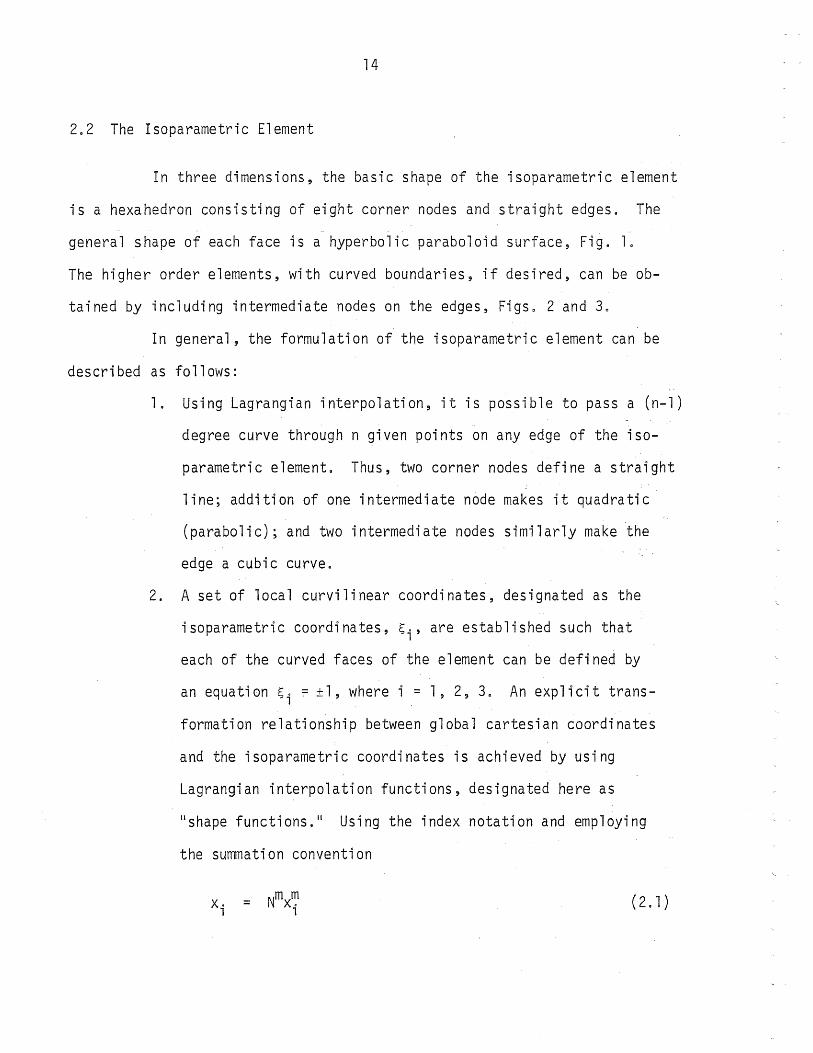
2.2 The Isoparametric Element
In three dimensions~ the basic shape of the isoparametric element
is a hexahedron consisting of eight corner nodes and straight edges. The
general shape of each face is a hyperbolic paraboloid surface, Fig. 1.
The higher order elements, with curved boundaries, if desired, can be ob
tained by including intermediate nodes on the edges, Figs. 2 and 30
In general, the formulation of the isoparametric element can be
described as follows:
1. Using Lagrangian interpolation, it is possible to pass a (n-l)
degree curve through n given points on any edge of the iso-
parametric element. Thus, two corner nodes define a straight
line; addition of one intermediate node makes it quadratic
(parabolic); and two intermediate nodes similarly make the
edge a cubic curve.
2. A set of local curvilinear coordinates, designated as the
isoparametric coordinates, ~i' are established such that
each of the curved faces of the element can be defined by
an equation ~i = ±l, where i = 1, 2,3. An explicit trans
formation relationship between global cartesian coordinates
and the isoparametric coordinates is achieved by using
Lagrangian interpolation functions, designated here as
llshape functions. 1I Using the index notation and employing
the summation convention
X. 1
= ( 2. 1 )

15
where
x. -1
= global coordinates (i = 1,2,3)
Nm = shape function at node m
m xi = coordinates at node m
(Superscripts and subscripts are used to denote the node
number and the direction of coordinates, respectivelyo
Therefore, x~ represents the coordinate at node m in the
direction.i; e.g., x1° denotes the y-coordinate at node 100)
Since each shape function Nm in Eq. 201 is a Lagrangian
interpolation function, it has a value of unity at node m
and is zero at all other nodes.
3. The displacement field in the element is defined in terms
of the nodal 'displacements by using the same interpolation
functions. Thus,
= Nm m u. u. 1 1
where
ui = displacements at any point in the element
u~ = displacement at nodem in direction i
(202)
Since both the global coordinates and the displacements
are expressed in terms of the same parameters (shape func
tions), the element has been designated as the llIso-Parametric ll
e1 ement.
2.3 Compatibility and Convergence
For a solution to converge monbtonical1y to:the true solution,tt is nec-
essary that the 'disp1.acements be continuous across the.interfaces between adjacent

16
elements. This condition is satisfied,if the displacement of any point
on an edge between the adjacent elements is uniquely defined in terms of
the displacements of the nodal points along that boundary line,and that
the boundaries of the adjacent elements fit with each other before any
deformation has taken place. Since the displacements and the coordinates
along the edge of an element are functions of the nodal dis~lacements and
the nodal coordinates, Eqs. 2.2 and 2.1, respectively, the compatibility
of the displacement between adjacent elements is satisfied.
Other conditions for convergence, i.e., the state of rigid body
motion and constant strain, are in fact implicitly insured in the isopara
metric formulation. This can be verified by showing that a displacement
field of the form
u. = a. + b . . x. 1 1 1 J J
(2.3)
is admissible in the displacement field as defined by Eq. 2.2. In Eq. 2.3
a,. and b .. are arbitrary constants. At node m, Eq. 2.3 gives 1 J -
m m m ( ) u. = a. + b . . x. 2.4 , 1 , J 1
where, each a7 has the same value as ai in Eq. 2.3. Substituting Eq. 2.4
into Eq. 202, one obtains
u. , m m m m = a.N + b .. N x. 1 lJ J
-(2.5)
If the displacement field given by Eq~ 2.3 is admissible, Eq. 2.5 must be
identical to Eq. 2.3. This can be shown by proving that the following are
i denti ti es :

17
a. = Nma~ 1 1
(2.6a)
X. = Nmx~ 1 1
(2.6b)
Equation 2.6b is identical to Eq. 2.1. In order to prove that Eq. 2.6a is
also an identity, a linear transformation of coordinate system x, into 1 .
another cartesian coordinate.system xi is considered.
x. = x. + a, 1 1 1
At node m, Eq. 2.7a gives
x'!l = 1!1 + a'!l 1 . 1 1
Substituting.Eqs. 2.7a and 2.7b into.Eq. 2.1,· one obtains
x. + a. = Nm (~ + a~) 1 1 1 1
(2.7b)
Or" (2.8)
= Nm m . I N lTHl1 -) a. a .. '1"',. x, - x. 1 . 1 1 1
Since the isoparametric coordinate system is unique to a givenele-
.ment,Eq. 2.1 holds for any global coordinate.system,.hence,
. x. = N~ 1 1
(2.9)
Substitution of.Eq~ 2.9 into.Eq~ 208 gives
which is the same.as.Eq. 2.6a.lfEq. 2.6a is.writtenin ordinary notation,
one obtains ENm =l~ with summation extended over all the nodes.

18
2.4 Generation of Polynomial Shape Functions
For various elements suitable polynomial which satisfy theneces
sary conditions of continuity can be written.by including only the. terms
which give the appropriate variation along the sides of the elements. For
example, considering the linear element, Fig.l,one can write
(2.10)
where
¢ = a component of the global coordinate or the displacement
vector at any poi nt in the element
r a. = constant coefficients
cr = functions.of isoparametric coordinates, ~i; thus, cl = 1, 2 8
c. = ~l' ... , c = ~1~2~3 EvaluatingEq. 2.10 at node m, one obtains
(2.11)
where
. Cmr = cr at node m
Equation 2.11 can be solved to obtain
(2.12)
Substitution.of.Eq. 2.12 into.Eq~ 2.10 yields

19
or (2.13)
,j.., Nm m 't' = ¢
where Nm is the requiredshape.function given by
(2.14)
In many cases,.it is possible to.write these functions.by inspec-
ti on· and· on·. the. bas is. of the. fundamental property of the· shape functi ons whi ch
has· been· stated in· Section 2.2, i .e.~ the shape· function for the node m, Nm,
is uni ty at node m and' zero at all other nodes. Thus, for an· ei ght node
element
(2~ 15)
in'which ~~ is the value of ~i at node m.
2.5 Higher Order; Elements':'
As· it has been indicated in· Section 2.2, the isoparametric family
of elements consists of various orders of elements· beyond the: linear' 8' node
· hexahedron.· A· higher· order element is obtained·.by· including' intermediate
nodes' on· the edges.· For: ins tance', a IIq uadra ti eel ement ll cons is ts of eight
corner nodes and· twe 1 ve i ntermedi ate nodes (one' on each edge), Fi g'. 2a. A
· Ilcubi c element ll is' obtained by' including' twenty-four intermedi ate'. nodes--
· two' on· each edge,' F; g'. 2b, and so· on. 'The· forego; ng examples'" however, are
special cases.of the· general· isoparametric element in'which'it is possible
to assign· anyorder~of:response' to~individual edges,· Fig,' 3.
Fi gure 4 shows a. typical edge',' AB,' under· various· degrees. of
'. responses.' When there~are: only two corner~nodes, A· and B, the~ response' is

·20
linear, Fig~ 4a.·Addition of· an· intermediate node results in both a para
bolic edge and displacement field. A set of shape functions, quadratic' in
the isoparametric coordinate along AS, say c;l' can be formulated for corner
nodes A· and B, and the intermediate node 1. This, however,would mean that
everyti me an addi ti ona 1 i ntermedi ate node is· introduced on any edge, a new
set. of shape functi ons . mus t. be used for the corner nodes. Thi s di ffi cul ty
is overcome.by defining the quadratic response on the edge as· the departure
.fr"'om linearity, thus r'etaining the linear response. defined by the corner
nodes.
where
( 2 .16 )
· ~AB = a component of coordinate or displacement vector,
· NA, NB
.. ¢A, ¢B
· t:. AB ¢
=
=
.. evaluated on edge AB
linear shape function for the corner nodes A and B
values.of ¢AB at node A and B, respectively
= ,the~quadratic departure of ¢AB from the linear re
~sponse defined~by,the'corner nodes
On thebasis.of known' chara~te~istics:of ~AB¢, i .e.~ it is qua~ratic~ and
vanishes at A and B (c;, =±l), one can write
· ~AB¢ (2.17)
where
(3 an· unknown' coefficient'which' is to be determined. for the
edge under' consideration ..
For' the corner node·A· on the·edge'AB,:Eq~ 2.15 becomes
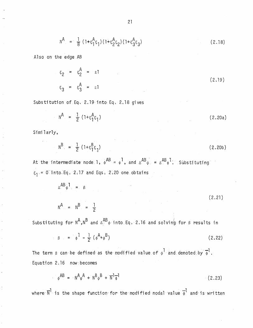
21
(2.18)
Also on the edge AB
~2 = ~A 2 = ±1
(2.19)
~3 = ~A = ±1 3
Substitution of,Eq~ 2.19'intoEq~ 2.18 gives
(2.20a)
Si mi 1 ar1y,
(~.20b)
At the intermediate node,l~ ¢AB = ¢1, and AAB 4', = ~AB¢l: 'S8bstituting
~1' = 0" 'jnto-:Eq ~ 2 ~17 and, Eqs ~ 2~ 20' one obtai ns
(2.21)
Substitutingfor'NA,NB and ~~B¢, into,Eq~2.16 and solvinb for S results in
(2.22)
The term scan, be, defi ned as the modi fi ed va 1 ue, of ¢ 1 and denoted, by ¢"1 .
, E qua t ion 2~ 16 now' be come s
¢AB:: 'NA¢A +'NB¢B + N'"¢l , (2.23)
'~ , 1 whereoN 'is the shape function' for the'modified' nodal value'¢" and'is'written

22
on the basis.of Eq. 2.17.as
. (2.24)
It can be seen that by substituting ~2 ~ ~~S. arid ~3 ~ ~~B for the edge AS
in.Eq. 2.24, N1 = (l-~i), which is in agreement with Eq. 2.17.
More intermediate nodes can be introduced on the same edge in order
to define a higher degree of response.~ Figure· 4c, forinstance~ represents
a cubic· response on· the· edge AS, which'has two intermediate nodes 1 and 2.
If there are I intermediate nodes defined· on· the same· edge, Fig. 4d, the
degree.of response~wou1d be (I+1) .. Equation2~16 can again be used to define
the total. response on the edge. The term 6AB~ represents the departure of
degree (1+1) from linearity. In a manner'similartoEq·. 2.17, it can be
wri tten' as
AB2 1 2 3 2 I 1-1 s s 6 ~ =. (1 -- S 1 ) (y +y ~ 1 +y ~ 1 + ... +y ~ 1 ) =y g (2.25)
The superscripts on. ~l in the above expression· represent exponential powers,
ySls' are asetof I unknown coefficients for the edg~ and gSi S' are I func
tionsof s1 . The'isoparametric coordinates for each of the I intermediate
. nodes· can.be substituted· in Eq. 2.25.· Thus,
(2.26)
. where,' ~!\B ~m and GniS are the va 1 ues: of 6AB~,and gS at themth intermediate
node, respectively. Solution of Eq~ 2~26 forys gives
(2.27)
Since the· set of ~-va1ues·.of I-inter'mediate nodes are replaced by the same

23
number of ¢"-values in Eq. 2.25, as before, -;pm's are designated as the modified
¢-values. The terms ~ are the shape functions corresponding to each of the
~-values, Eqso 2025, 20260 It can be seen from Eq. 2026 that on edge AS,
AS) i\'i'lll m s3=s3 ,N :: 9 , which is in conformity with Eq. 2.24.
It should be noted here, that arrays Gmn and Hmn , Eqs. 2.26 and 2.27
are cons tant for a gi ven number of i ntermedi ate nodes and they are independent
'of the position or direction of the edge. Itis, therefore, possible to
compute and store them at the beginning of the program for future use.
2.6 The Element Stiffness Matrix
With the given displacement field for the element,.Eq. 2.2, it is
possible to obtain the stiffness matrix using the principle of virtual dis
placement and the constitutive' relations of the continuum.
In a cartesian. space, the strain tensor is given by
1 (
dUo au QJ _, +_J "2 ax. ax.
J 1
Eo. :: lJ
Differentiating Eq. 2.2 and substituting into.Eq. 2~32, one obtains
E •• lJ
in whi ch
:: Zm um ijk k
where, 0ik is the Kronecker delta.
(2.32)
(2.33)
(2.34)
The shape functions Nm, are expressed in terms of the isoparametric
coordinates. In order to evaluate their derivatives with respect to the
g1 oba 1 coordi nates, one needs the trans formati on re 1 at; onshi p between the

24
cartesian and the isoparametric coordinates. This relationship can be
obtained by differentiating Eq. 201 with. respect to ~.o . J
(2.35)
The required transformation 8Xo
matrix~, Eqo 20350
8~ • array dX~ is obtained by inverting the Jacobian ,
(1 s 0
The global derivatives of the shape functions Nm, J
Eqo 2034, can be evaluated now by
(2.36)
The stresses are related to strains.by
(2.37)
where E "0 is the mater; al property tensor. pQ1J If the element is given a virtual displacement ou~, the corre-
sponding change in strain can be computed fromEq~ 2~33.
The internal work associated with the virtual displacement is
oWint = ~aij OE jj dV v
(2.39)
and the external work of the nodal forces through the nodal virtual dis-
placements is
oWext p~ ouf!1
1 1 (2.40)
For a system in equilibrium 8Wint = oWextO Equations 2.33, 2.34, and 2.37
to. 2 0 40 9i ve

25
m mn n Po;: k a 0 u" 1 lJ J
in which k~~ is the element stiffness matrix* which is given by lJ
kf!1~;: J E dNm
aNn dV ij . ikjQ, dXk axQ,
v
where
(2.41 )
(2.42)
(2.43)
For the elastic isotrop'ic material, the material property tensor
EikjQ, can be expressed explicitly in terms of the Lame's constant A, and the
modulus of rigidity~.
(2.44)
substitutingEqo 2.44 in Eq. 2042 one obtains
J A 8Nm
aNn +].l(ClNm
aNn 0., + 8Nm aNn) dV 8xo 8X. 8Xk 8Xk lJ ax. ClX.
v 1 J J 1
k~~ ;: lJ (2.45)
A numerical integration scheme for computing the stiffness matrix
is given in Section 20 80 It was found during the study that the index nota-
tion formulation of the stiffness matrix results in an economic organization
of computation. In addition, in case of homogeneous material in which the
terms of material property tensor are independent of position coordinates,
a further reduction in computer time is achieved by taking the material prop
erty tensor E'koA outside' of the integral sign,Eq. 2.42. A more detailed 1 J x,
discussion on this subject is given in Appendix A.
* Since k~j is a four-dimensional array; it cannot be defined by the term .1l.ma trix. 1I Nevertheless, the term "stiffness matrix" is conventionally used to define a.relationship between the nodal forces and the nodal displacements, and is used in the study.

26
207 The.GeneralizedLoads
In the discrete formulation.of continuum problems, the.applied
loads must.be transferred to nodal points, where the displacements are de-
fined" This transformation is best achieved. by using an energy. approach
similar to that used for obtaining the element stiffness properties. The
nodal1oads so obtained are referred to as the generalized loads.
The applied. loads may either be concentrated loads.acting at any
point,or they maybe distributed over a continuous domain, such as a volume,
an area.or a length.
207.1 Concentrated Loads
. The.equavalent nodal loads resulting from a concentrated load Q~
acting at point A (~i = ~f) are obtained.by.equating the work of both the
nodal and the concentrated loads through a virtual displacement. Thus,
where m
p~ = ., desired generalized load
aUo = virtual displacement field 1
ThetermNm(~f) represents the value of Nm at point A.
8U~ are arbitrary displacements,.Eq. 2~46 yields 1
2.7.2 Distributed Loads
(2.46)
Since, cUe and thus 1
(2.47)
Ina procedure similar to that for the concentrated loads, for a
distributed load.of intensity qi acting on a domain 0, the.equivalent nodal
loads are obtained from
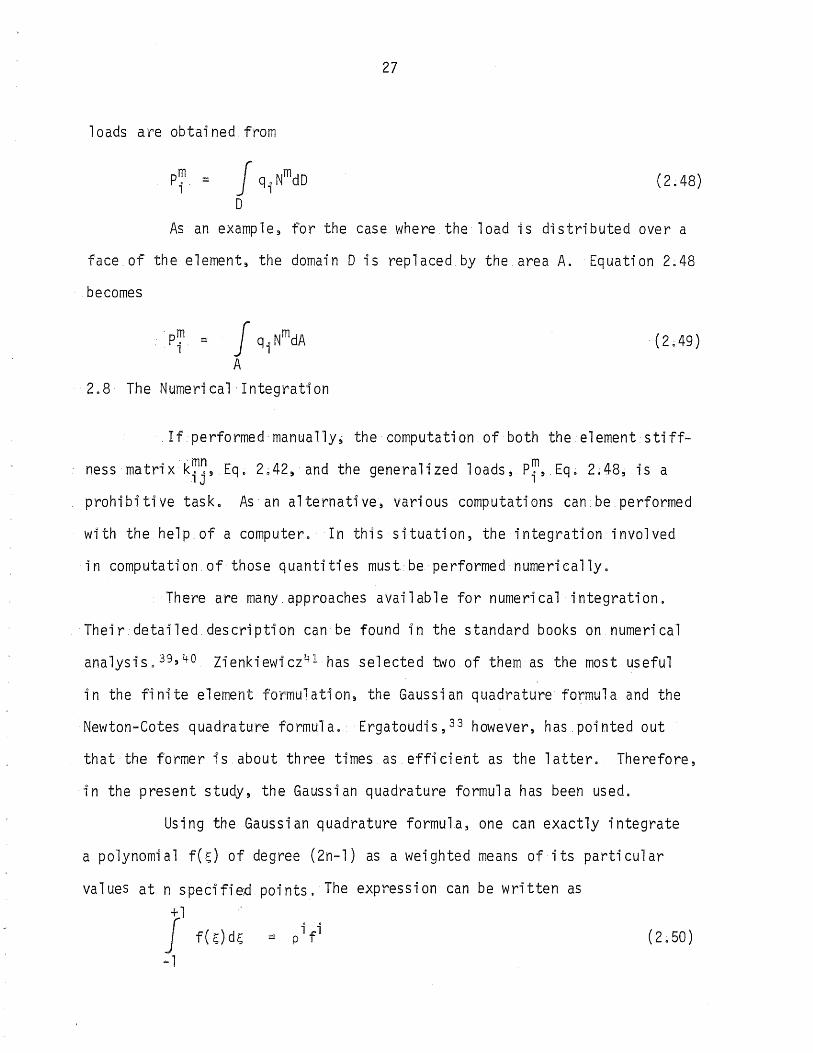
P~ ~ J q;NmdD
o
27
(2.48)
As an example, for the case where the load is distributed over a
face.of the element, the domain 0 is replaced by the area A. Equation 2.48
becomes
P~ = J q;NmdA
A
2.8 The Numerical Integration
.If performed manually; the computation of both the element stiff-. ··mn "m. ness matrix k .. , Eq. 2~42, and the genera11zed loads, P.,Eq. 2~48, 1S a
1 J 1
prohibitive task. As an alternative, various computations can be performed
with the help.of a computer. In this situation, the integration involved
in computation of those quantities must be performed numerically.
·There are many. approaches available for numerical integration.
Their detailed. description can be found in the standard books on numerical
analysis. 39 ,4o Zienkiewicz41 has selected two of them as the most useful
in the finite element formulation, the Gaussian "U..,A"" ... -i-.,,,,,r\ +J"'\'Ii"m'·" ~ y aural.u/c: IUIII~'U and the
Newton-Cotes quadrature formula. Ergatoudis,33 however, has.pointed out
that the former is about three times as efficient as the latter. Therefore,
in the present study, the Gaussian quadrature formula has been used.
Using the Gaussian quadrature formula, one can exactly integrate
a polynomial f(~) of degree (2n-l) as a weighted means of its particular
values at. n specifie;cl points. The expression can be written as +1 J f(~)d~ = pifi
-1
(2.50)

28
where i
p - the weighting coefficients, and
fl ~ the value of function f(~) at n specified points (~=ni)
I n two di mens i ons ~ the integral becomes +1 +1
J _,/(' -1 -1
'f'(~ ~ ·)d~ dr - i_jfij 1;1;1;2 ~1 1;2 - P (J
and in three dimensions, it is
+1 +1 +1
J Jr J f ( ,.' r C -) d r de d>- i j k fl j k <;1 ~1;2'~3 1;, ~2 1;3 ;; 0 0 P
-1 -1 -1
(2.51 )
(2.52)
The pi and ni values for different orders of Gaussian quadrature:are readily
obtainab'leo 39 ,!4o, In the present study, as was also found by other investi-
gator~,37 integration carried with the 4th order Gaussian quadration is con-
sidered to be sufficiently accurate to handle all problems.
209 The Load-Displacement Equations for the Structure
In the displacement method of finite element analysis, the pro
blem always reduces' to the solution of a set.of simultaneous equations,
referred to as the load-displacement,equation. In matrix notation,
KU :: F (2.53)
where
K = the nonsingular structural stiffness matrix
U ;;;: the vector of unknown displacements, and
F :: the nodal load vector
Solution of Eqo 2053 yields the unknown displacementsU, which upon substi
tution into the strain-displacement relation~ Eq. 2.33, and subsequent use

29
of stress-strainrelation,Eqo 2,37, gives the desired stresses.
Various steps in arriving at,Eqo 2.53 are discussed in the follow-
ing.sections,
2090' Assembling the Structural Stiffness Matrix
The structural .stiffness matrix'is obtained on the basis of the
principle of virtual' displacement. The total ,virtual work done on the
,structure,consistsof,the virtual work contributions of the individual ele-
ments" The s tructura 1 s ti ffnes s matri x. is obtai ned by, s ummi ng ,up the s ti ff ..
ness matrices ,of the contributing elements. Thus,
where
the stiffness matrix of the unconstrained structure
kr = the stiffness matrix of the element r
M = the total number: of, elements
The stiffness matrix obtained in,Eq. 2.54:isused,to obtain the
'load-displacement relationship for the unconstrained structure.
K lJ :: F (2~55)
'where IT and f are the vectors of nodal' displacements and loads"respectively,
for the unconstrained structure.
Without any constraints, a structure,is free to undergo rigid,body
motion; therefore, there is no unique solution to,Eq. 2.55. Mathematically,
this phenomenon manifests itself,by the singular nature of the stiffness
matrix K. Nevertheless, all stable structures are provided with enough dis
placement constraints to.prevent rigid body motion. A nonsingular stiffness

30
matrix K can be obtained from the singular stiffness matrix K by incorpor
ating those constraints in a manner explained in the next section.
2~902 Displacement Constraints
Some of the constraints envisaged in the preceding section can be
in the form of zero nodal displacements in given global directions at cer
tain joints. If there are no other constraints~ the nonsingular stiffness
matrix K can be obtained from the assembled stiffness matrix K, Eq. 2.54,
by omitt'ing the t"OWS and the columns corresponding to the constrained dis
placements '0
Another" type of constraint often encountered is in the form of
a set of explicit relationships between two displacements, say U, and U2,
such as
(2.56)
where C is a known constant. For instance, constraints defined by Eq. 2.56
exist when the displacements are zero in the direction normal to a boundary
which is inclined to the specified coordinate axes, Fig. 5~. If the bound
ary is parallel to x3 ax.is and makes an angle e with the Xl axis, then
C = cot e~ in Eq. 3.56, where U, and U2 now represent the displacements in
Xl and x2 directions, respectively, at a node on the boundary.
In the case of a medium thick plate subjected only to lateral load,
Figo 5b,' denoting the displacements in xl' x2~ x3 directions by u1 !) u25 u33
respectively, and using superscripts t and b to denote the top and bottom
layers, the following relationships are easily obtained!

31
t b u1 - -u,
t b (2.57) u2 - -u2
t b u3 - u3
Equations 2~57 are also of the type of Eqo 2056.
Wi th the g1 yen cons trai nts, i n general, a re 1 ati onshi p between
the displacement vectors of the unconstrained and the constrained structure
can be written as
"IT = TU
where T is a geometric transformation matrixoOn the basis of,the principle
of contragradience,42
F = (2.59)
Substituting.Eqo 2058'into Eq. 2~55, and substituting the. resultant expres
sion for fintoEqo 2059, one obtains
F = (TT K T) U (2.60)
Comparison ofEqo 2.53 and 2060 yields
(2.61)
which is the desired expression for the nonsingular structural stiffness
matri x.,
In mos teases, the geometri c trans formati on matri x T of Eq ~ 2 ~ 58
·isonly.sparsely-filledo Computations for:Eq~ 2~61 'can~ therefore~ be

32
organized economically without actually performing direct matrix multipli
cati on 0
2.9.3 Solution of the Load=Displacement.Equations
As has been mentioned earlier in this section, in the displacement
method of finite element analysis, the problem always reduces to the solut·ion
of a set.ofsimultaneous.equations,.Eq. 2.53. Invariably, an efficient
method of·solvingequations takes into account the symmetry and the banded
nature of the stiffness matrix. In the present study, only the upper tri
angular portion of the stiffness matrix is considered, and a variable band
width approach has been followed. The resulting banded upper triangular
matri x has been stored ina co·l umn array in order to economi ze the storage
requirementc The solution of the equations is based on the Gaussian elimin
ation method. 43
The method of solution followed in this study is quite efficient
forsolvtng a banded set of equations. However, in three-dimensional pro
blems the band width of the individual equations tends to be very large,
thus requiring a large storageo In addition, one has to operate on many
zero terms within the band,which adds to the cost of equation solving. The
frontal method44 is an improvement in this respect. In this method, only
that part of the stiffness matrix which corresponds to the current active
variables in the "front" is stored in core, thus making a substantial saving
on the core requirement. In general, the size of the front is smaller than
the band width of the equations, which in effect, eliminates a good number
of zeroes from the process of computati on 0 Thi s res ul ts in economy of the
computer time. On the other hand~ the frontal method uses several input
outputoperationso For this reason, in many problems, a straight, variable

33
band width approach (used in this study) may prove to be more·economical .
. Several other methods have been used for the solution of simul
taneous equations. The so-called "square-root method" 45 is one which has
been used extensivelyo The method consists of decomposing the stiffness
matrix into a product of a lower triangular matrix and an upper triangular
matrixo A similar method has been used in the general purpose finite ele
ment program NASTRAN ~~6

Chapter 3
PLASTIC ANALYSIS
3.1 General
As is well known in the elastic deformation,strains are related
to stresses by a holonomic relationshipo An elastic process is also revers
ible. On the contrary, the phenomenon of plastic deformation implies that
the state of strain is not uniquely determined by the state of stress--it
is path dependento Also, the process of plastic deformation is irrevers
ibleo This means that the work done during a plastic action cannot be
recoveredc
Most materials behave elastically up to a certain stage of load
ing, beyond which plastic deformations take place. In a uniaxial state
of stress, the stage·at which yielding starts can be determined easily
from the experimental stress-strain curve. In multiaxial state of stress 9
however, there are i nfi ni te number of poss i b 1 e combi nati ons of stresses
at which yielding starts. A unified basis of establishing all such com
binations is known as the yield criterion. Another necessary considera
tion in constructing a plasticity theory is the incremental relationship
between stresses and st'rains in the plastic range. Both the yield cri;..
terion and the plastic incremental stress-strain relationship are discussed
in the followingsectiono
302 The Yield Criterion and the Flow Rule
The yield criterion is described by a.hypersurface (designated as
the yield surface) in six-dimensional stress,spaceo 47
34

35
(3.1)
where
~ ~ the loading function, and
K = the yield function.or the work-hardening function
For a given prey; ous . deformation hi story ,~(01' . ) is a function of the cur. J
rent state.of stress and K is a constanto If the state of stress is such
that it lies on the yield surface. described byEq. 2.1, initiation of
plastic deformation can take placeo
For a perfectly plastic material~ the jield surface, Eqo 3.1,
remainsconstanto However,for a strain hardening material, the.yield
surface must change with continued straining beyond the initial yield .. This
phenomenon is incorporated inEq. 3.1 .by allowing both ~ and K.to.befunc-
tions of the state of stress and the plastic deformation history .. Thus,
every time yielding takes place, K takes on a new value. If the material
is unloaded and then loaded again, additional yielding does not take place
unless the current value of K has been exceeded.
As has been mentioned earlier, in general, ~ is the function of
both, the state of stress and the deformationc A good deal of analytical
simplification is achieved by neglecting the Bauschinger effect;48 assum
ing that the material 'strain hardens isotropically.Such an assumption is
approximately true if the load is applied monotonically.49 It should be
noted that a basic assumption in the plastic analysis is that the loading
function ~(aij)existso
Various incremental stress~strain equations, or the so-called
flow rules have been suggested for analysis in the plastic range. 47 Most

36
of them implicitly assume that the infinitesimal stresses and strains are
related linearly~ A unified approach for arriving at the incremental
stress-strain equat1on~ as presented by Drucker~50 is followed here.
Drucker postulated the implications of work hardening and the
ideally plastic material~ and established that the plastic strain incre~ tl U
ment~ dSij~ is proportional to the stress gradient of the yield surface.
Ii
dEij (3.2)
where
d), ;:: a positive incremental constant of proportionality
,"Equations 30' and 302 form the basis of the development of the
method of p~lastic analysis discussed in the following sections.
3.3 Incremental Stress-Strain Equation
In the plastic range~ the relationship between stresses and
strains .is non'linear and also path dependent (see the preceding two sec
tions)c In order to perform a plastic analysis, the loading path is dis
cretized into several linear load steps. The increments in stresses and
strains for each step are then related by the rate constitutive laws. The
assumption is that the extension of the linearized steps is small so that
the change in stresses during a particular step can be regarded as infin-
itesimal and Eqc 302, which is true for infinitesimal increments of stresses
and st'rains~ can be employed for small finite increments.
The total strain increment dSij is the sum of the increments in ~ I I
elastic and plastic strains dSij and dsij , respectivelyo
(303)

37
The re 1 ati onshi p between s tresses and e 1 as ti c s trai ns is g1 ven by Eq. 2.37
which is modified for incremental stresses and elastic strains as
tt
dOij = Eijk1 d~kt (3.4)
M
Substituting dsk£ from Eqo 303 into Eqo 3.4 and subsequently making use
ofEqo 302, one obtains
(3.5)
It has been stated in Section 3G2 that the yield function K,
Eq. 301, is a function of the state of stress and the plastic.deformation
pathc For many materials an.equivalent statement is that theyieldfunc
tion is a.function of the plastic workWP. Thus,
K (3.6)
where
. P i i
dW ;::; 00' ds. 0
lJ lJ (3.7)
Obviously, even. for those materials which satisfyEq.3.6, the yield func
tion continues to:be a function of the. state of stress and the plastic
. deformation. path since wP is a function of the state.of stress and of this
pa th, . Eq c 30 70
Making use of Eqso 3.2, 3.6 and 3.7, the complete differential
ofEq~ 3.1 can be written as
dlJ! -~ deL Q ;: rdA dO col J
'1 J (3.8)
where
38
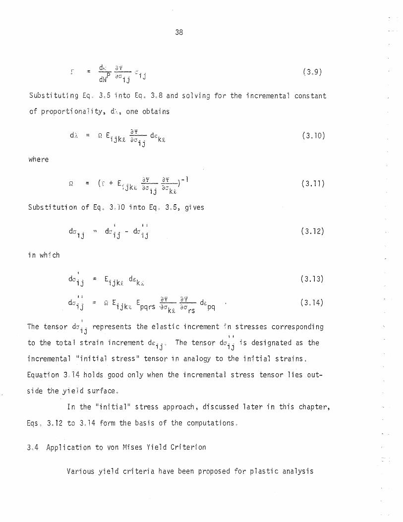
substituting Eqn 3,5 into Eq. 3:8 and solving for the incremental constant
of proporti anal i ty, d:\ ~ one obtai ns
where
3Y! d>~ ;::; n Eu Ok' ~,.. ~ dsk"
1 J ~ d0o, 9-1J
(, ;-":.' + 80/ 'dip" -1 Ed Q,. i., -." ---) lJkx .. dOo 0 de:- "
1 J klG
Substitution of £qc 3010 into Eqo 3.5, gives
in wh'l ch
!
doo" lJ
II ~
do-.. , lJ
u
(3.10)
(3.11)
(3.12)
(3.13)
(3.14)
The tensor dOij represents the elastic increment in stresses corresponding ! !
to the total strain increment dEijo The tensor dUij is designated as the
incremental Ilinitial stress ll tensor in ana10gy to the initial strains.
Equation 3014 holds good only when the incremental stress tensor lies out
side the yield surface.
In the "initia'jll stress approach, discussed later in this chapter,
Eqsc 3.12 to 3.14 form the basis of the computations.
3~4 Application to von Mises Yield Criterion
Various yield criteria have been proposed for plastic analysis

39
of solids having different material.propertiesc 47 The.von Mises.yie1d cri
terion explains the behavior of a wide class of ductile materials very
closely. The Prandtl-Reuss equations form the flow rule associated with
the von Mises yield criterion.
For the von Mises yield criterion,.Eq. 3.1. reduces to
(3.15)
in whi ch
(3.16)
and
2 K := a e (3. 17)
where S. a
lJ is the deviatoric stress tensor and is given by
Suo 1 :;:;; Go a - "3 akko ij lJ lJ
(3.18)
It is seen from Eq~ 3~15 that for a uniaxial state of stress~
where the only nonzero co~ponentof stress tensor is a", one obtains
(3.19)
By the ana10gy represented.by.Eqo 3.19, ae is designated as the effec
tive stress {equivalent to the uniaxial state of stress).
Differentiating Eq. 3.16 with respect to Go 0, one obtains lJ
8lJ! d0., a
lJ ;:;; 3 So 0
lJ
Substitution of Eqo 3.20 into Eq. 3.2" yields
o H
ds co;; 3 S. a di\ 1 Jl J
(3.20)
(3.21 )
40
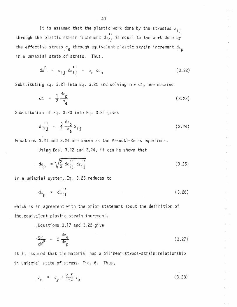
It is assumed that the plastic work done by the stresses Gij Ii
through the plastic.strain increment dS ij is equal to the work done by
the effective stress a through equivalent plastic strain increment dsp . e
in a uni axi al state of stress 0 Thus,
-WP ! I
d . '= 0" 0 0 dS ij = ue d;- (3.22) lJ -p
Substituting Eq. 3.21 intoEq. 3022 and solving for d~,oneobtains
( 3.23)
Substitution ofEqo 3023 into Eq. 3021 gives
(3.24)
Equations 3021 and 3024 are known as the Prandtl~Reuss equations.
Using.Eqso 3022 and 3024, it can be shown that
(3025)
In a uniaxial system, Eqo 3025 reduces to
(3.26)
which is in agreement with the prior statement about the. definition of
the.equivalent plastic strain incremento
Equations 3.17 and 3022 give
(3.27)
It is assumed that the material has a bilinear stress~strain relationship
in uniaxial state of stress, Fig. 6, Thus,
(3.28)

41
where z is the strain hardening coefficientcDifferentiating:Eq. 3.28 with
respect to sp' one obtains
do e z E d-:::
p;;;; 1 ~Z (3.29)
Substitut1ngEq~ 3029 into.Eq, 3.27 and substituting the resu1tingexpres
sion together with.Eqo 30 20 into Eqo 309, one gets
2 z E :;:; 4·,..,.-vel'"" z
Substit~tion of.Eqs~ 2044, 3.20 and 3.30 into.Eq. 3~10 yields
:: ._. 1_ (_z_. E + 311)-1 402 1-z
e
·Substituting.Eqso 30 13, 3020 and 3031 ·into.Eq~ 3.14 one obtai~s
where
D tl
dao 0
lJ z E )-1 cb e
- (1 + 3(1-z)u Sij ~
It should be noted that Eqso 3.32 and 3~33 are applicable only when
(3.30 )
(3.31 )
(3.32)
(3.33)
Eqo 3.15 is satisfied in the beginning of the increment, i .e.;when the
state of stress lies on the yield.surface. Also dO' should always.be . e
positive.or.zeroo
The loading function, as defined.by.Eq. 3~16~ is .quadratic in
stresses. For the sake of convenience in forthcoming discussion, a
1I1 0ading stress 'l
(3.34 )
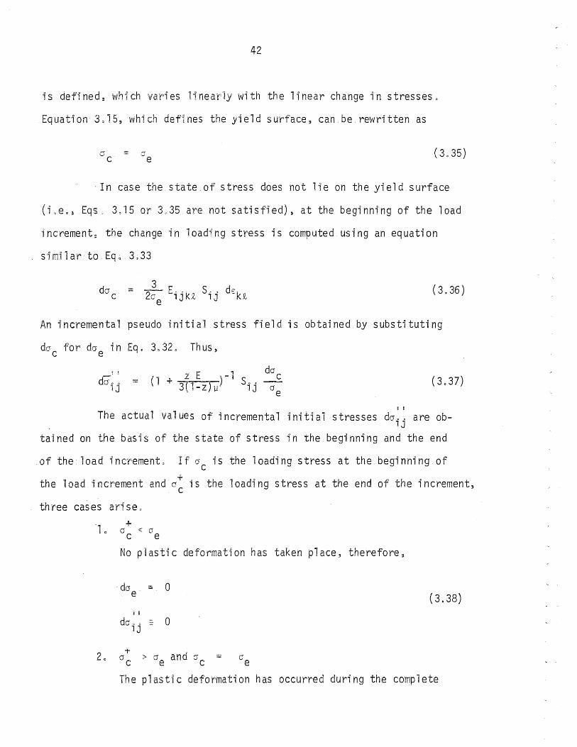
42
is defined~ which varies linearly with the linear change in stresses.
Equation 3,15, which defines the yield surface, can be. rewritten as
a C
. In case the state.of stress does not lie on the yield surface
(iae.~ Eqs, 3015 or 3.35 are not satisfied), at the beginning of the load
increment, the change in loading stress is computed using an equation
similar·to.Eq~ 3~33
(3.36 )
An incremental pseudo initial stress field is obtained by substituting
doc for dOe in Eq. 30320 Thus,
( - z E )-'1 1 + 3(1-z)u Sij (3.37)
i i
The actual values of incremental initial stresses da .. are oblJ
tained on the basis of the state of stress in the beginning and the end
of the load incremento If 0c is the loading stress at the beginn1ngof 1-the load increment andere is the loading stress at the end of the increment,
th'ree cases ariseo
No plastic deformation has taken place, therefore,
da :=:: 0 e (3.38) l U
do" 0 lJ - 0
2c + and °c > °e (J :;;:;
° c e
The plastic deformation has occurred during the complete

43
1 oadi ng increment 0 In thi s cas e,
(3.39)
+ Gc > c e and 0c < 0e
Only part of loading increment has caused plasticdeforma-
tions. Since a linear problem is solved for each loading
increment, one can write
dOe = d--.... ' c - (oe - 0" c)
da (3.40 ) U! 8 I
de 0 0
e de, 0 ;::::; cr:;-.
lJ t.·'c lJ
. Equations 3034 to 3040 are used in applying the initial stress
approach to the isoparametric element. The significance of the above
treatment.becomes more obvious in Section 3070
3.5 Method of Analysis
As has been mentioned in Section 303, an incremental loadingap-
proachmust be used for the analysis in the plastic range of material
behavior. The incremental equations 1n the preceding two sections are
written in differential notations which imply that the increments are in-
finitesimally smal10 However, in practice one must use finite increments.
It is assumed that the relationships, which are true for infinitesimal in-
crements, can be applied for small finite increments, In order to dis-
tinguish between the infinitesimal increments and the finite increments 9
the differential operator IIdll will be replaced by 116" in the further

44
treatment •. For instance, j0ij will denote a finite increment in the stress
tensor (\ i j 0
~ One of the earlier methods which follows the incremental loading
approach is the lIinit1al str'aln" methode 51 An elastic problem is solved
for each increment of load1ngo An estimate of the plastic strain for the
loading increment is made and this assumed plastic strain is treated as
the initial straino A loading system "equivalent" to the initial strain
is evaluated and is.applied on the structure in order to solve another
elastic probleme The iterative process consists of determining the ini
tial strains, evaluating the.equivalent loading and solving the elastic
problem. The convergence is assumed to have been reached once the initial
strains become negligible within a given tolerance.
A serious drawback of the initial strain method is that it applies
on'ly to mater'ials showing a pronounced degree of strain hardening. When
the strain hardening is either very small or zero, very large plastic
strains are caused by small increments of loads, resulting in a poor con-
vergence c
Ahother approach to the finite element incremental plastic anal~
.ysis is the quadratic programming method. 17 ,lB The incremental problem is
solved "exactly" in a finite number of iterations for both work hardening
and perfectly plastic behavior', However, computer programs for large
scale quadratic programm1ng problems are not readily available. Moreover,
the application to finite element models with nonconstant stresses and
strains in each element presents some complications"
A third incremental method of plastic analysis is the tangent
stiffness method~s2,5S In this method, at any loading step, the incre
mental stress~strain relationship is used to determine the stiffness

45
matrix of. the element which has undergone a plastic deformation. Such a
stiffness matrix is designated as the Iitangent stiffness matrix.1I For
each loading increment, an elastic problem is solved using the tangent
stiffness matrix. of the structure c For elements which have undergone
further plastic deformation, the state.of stress.in the element and thus,
the incrementalstress~strain relation for the element have changed. A
. new tangent stiffness mattix is evaluated and the problem is. resolved.
This process is continued for each loading increment until the structure
becomes very flexible due to widespread plastic deformations in critical
zones such that the displacements become unbounded.
Since, for each loading increment, a new stiffness matrix is
computed for the element which has undergone plastic. deformation, the
equilibrium equations at every joint which is incident on that element
must be modified o Both the recomputation of the element stiffness matrix
and modifications of equilibrium equations constitute a major computational
effort, .especial1y for- the three-dimensional, isoparametric element .. For'
this reason 3 a more economical method of incorporating the plastic material
behavior, the initial stress method S14 is considered in this study.
In this method of analysis, for each loading increment, the pro
blem is solved elastical1Yolf any point has undergone plasticdeforma-
tion during the loading increment, the increments of stresses and strains
at that point will not satisfy the incremental stress-strain relationship, * ! I
Eqo 3c12" In or'der to satisfy Eqo 3012, a set of stresses 6O'ij , Eq. 3.14,
are calculated and subtracted from the elastically evaluated stress incre-I I
ment, Eqo 30130· In analogy to the initial strains, the stresses 60' .• can lJ
* The equations referred to'here should be considered as applied to finite increments.

46
be called incremental Ilinitial stresses. '1 Equilibrium is restored by ap-
plying a set of loads on the structure equivalent to the incremental ini
tial stresseso A new elastic problem is then solved with the new loading.
An iterative scheme is used which' consists of evaluating the inftial
stresses,. applying the equivalent set of loads on the structure and carry
ing a new elastic analysis, The iterative process is continued until the
set of loads equivalent to the computed incremental initial stresses be
come sufficiently small.
Figure 7 shows the graphical representation of the initial stress
method on a two-dimensional stress planeo
The initial stress method is economical since the original
stiffness matrix of the structure is not changed during the analysis. The
Gaussian elimination procedure for reducing the stiffness matrix of the
structure to an upper triangular matrix coefficient is performed only once.
As ,opposed to the initial strain method, this method can be applied to
materials with , zero or small strain hardening, since for any state.of
strain the state.of stress is uniquely defined.
306 The Incremental Load-Displacement Relationship
An incremental load-displacement relationship can be developed
in conjunction with the initial stress method of plastic analysis discussed
in the preceding section, The incremental strain-disp1acement relation-
ship can be written on the basis of Eq, 2.330
(3.41)
47
The incremental stress-strain relationship is given by Eqo 3.12; it can be
rewritten with the help of Eq. 3.13 as
I I
!::,O 0 Q
lJ ~ Eijk~ 6Ek~ - ~Oij (3.42)
The incremental load-stress relationship is obtained from Eq. 3.41, using
the principle.of contragradience. 42
L\P mk ;: f zf!1. k ~0 o. dV lJ lJ
(3.43) V
Combining Eqs. 3041 to 3.43, one obtains the desired incremental load-
displacement relationship for an element
6Pf!1 = k~~ ~u~ - ~p~' I
1 1 J J 1
where k~~ is the elasti'C stiffness matrix, Eq. 2.42, and lJ
(3.44)
(3.45)
! I
The vector 6pr is designated as the incremental initial load vector.
The incremental load-displacement relationship can be obtained
by proper summation of Eqc 3044 over all the elements in a manner similar
to that discussed in Section 2.9. Using matrix·notation
i i
~F = K ~U - ~F (3.46)
i I
The vector~F in Eq. 3.46 denotes the incremental initial load vector
for the structure.
Equation 3046.represents aset of nonlinear simultaneousequa
tions. The nonlinearity stems from the fact that the incremental initial ! I
load vector 6F is a function.of the state.of stress which in general
does not remain constant during a loading increment.

48
For a given loading increment,.Eq. 3.46 can be solved using a
modifiedNewton~Raphson approach. 42 First, an approximate value for the
incremental displacement vector 6c U is obtained by solving the linear
equation
.6F ;: K ~oU (3.47)
Using the approximate value of the incremental displacement vector ~oU, I H
an initial"load vector ~C!F is calculated (see Eqs. 3.44 and 3.46). A
linear system of. equations,
( 3.48)
is solved for a set of corrections 6'U in the incremental displacement 1 ! I
vectoro An incremehtal initial load vector 6 F is computed and another
set of equations similar toEqQ 3~48'is solved. At the ith iteration,
thefte ldequati on cah,be.wri tten as
(3.49)
The iterations are.terminated when the incremental initial··load.vector o R H
~lF has . become sufficiently small. The total increment in the displace-
ment vector is given.by
i \' "rU t:.U =: I L.I
r~O (3.50)
The same procedure is followed for the analysis.of other loading increments.
Figure 8 illustrates the Newton-Raphson method schematically for
a uniaxial loading.;

49
3.7 Application to the Isoparametric Element
The iterative scheme, as explained in the preceding,section, can
be applied to any finite element provided a suitable way of defining the i I
incremental initial stress field iJcc, is available. In a partially yielded lJ
element, the elasto-plastic bounda'ry divides the element into two portions.
The va'lue of L,J ij will be zero in the unyielded portion and it will have a
nonzero value in the portion which has been yielded.
The initial stress field is used in Eqo 3.45 in order to compute
the equivalent nodal loads. In the isoparametric element, the volume inte
gral on the right-hand side of Eqo 3045 is evaluated numerically. There-1'1
fore, it is s uffi ci ent to know the value of l\Oij at the poi nts of i ntegra-i I
ti on on'1y. In order to compute the value of 60ij at any point usi ng the
incremental form of. Eq. 30 14, one needs to know both the current state of
stress and the state of stress at the beginning of the loading increment.
This means that the stresses must be computed at eachpO,nt ofinfegrafiOn
within an element and stored for future use for each loading increment.
Computing and storing stresses for several poihts of integration
in each element is an expensive process. Moreover, the stress field which,
in this case, is ,defined as a function of nodal displacements within an
element, is not continuous across the elementboundarieso This may force
some,of the element boundaries to become the elasto~plastic boundaries in
the continuumo Therefore, in view of these drawbacks, a "stress-interpo-
lation". approach is employedc
In the stress-interpolat1on, approach, it is assumed that the
averaged nodal stresses are reasonably accurate representati ons of the
state of stress at those points. It is further assumed that any stress

50
field can be defined as an interpolation of averaged nodal stresses in an
element o Thus, a stress field can be defined as
where
¢ = a component. of the stresses m ¢ = value of ¢ at the element node m
( 3.51 )
Nm. = interpolation function for node m, same as the shape
functi on us ed in Eq 0 201
The state of stress is examined'at each node in order to. deter-
mine whether it has undergone a plastic deformation during a particular
loading increment. An element is partially or fully plastic if some or
all the nodes in the element have undergone a plastic deformation.: For a
plastic element, the incremental pseudo initial stresses are calculated at
each node of the element using.Eq~ 3~37.· The incremental pseudo initial
stress field in the element is then defined according to.Eqo 3.51.
(3.52)
Similarly; the loading stress Gc and the effective stress Ge at any point
within the element are obtained from
(3.54)
Once the incremental pseudo initial 'stresses, the loading stresses and the
effective stresses have been computed at the integration points, Eqs. 3~52 -
3~54; the incremental initial stresses for these points can be obtained

51
Having determined the incremental initial stresses at the inte
gration points, the computation of incremental initial loads and the iter
ative solution of the resulting set of equations is carried out in the
manner explained in Section 306,
308 Summary of the Pl asti c Analysis
The initial stress method has been used for analyzing the struc
turein the plastic range, The fundamental approach of the method has
been outlined in Section 3 0 5 0 The nonlinear set of load-displacement
equations has been obtained in Section 306. It is shown that the iterative
procedure followed in the initial stress method is a modified Newton
raphson method for solving nonlinear simultaneous equations. The.method
is adaptab 1 e to any fi ni te e1 ement provi ded a procedure is set up to de
fine the incremental initial stress field within the element. A stress
interpolation scheme is suggested in Section 307 for applying the method
to the isoparametric element.
The computational procedure for carrying out the plastic analysis
using the initial stress method is summarized belowo
'0 Initiation of yielding
ao Apply the specified set of loads and determine 0ij
and Eij
bo Calculate the loading stress 0c for all the nodes.
Obtain the highest value of 0 C ' say 0c/max' The
scale factor s to initiate yielding is
s= ° / c max

52
Co Apply the scale factor to the applied loads, displace-
ments, strains and stresses in order to determine their
state at the initiation of yielding
20 Elasto-plastic analysis
aoApply a specified fraction of the yield load as the
b.
D
next loading incremento Compute 60, . and 6s, e at all lJ lJ
the nodes on the basis of an elastic analysis fi
Add DO, 0 and /J.s, 0 to existing values of 000 and s.", lJ lJ lJ lJ
respectively, to obtain the current values of 0.0 and 1 J
so. lJ
+ Co Compute the current value of the loading stress 0c and
examine the state of plastic deformation at all the
nodes
de Compute the incrementa'l pseudo initial stresses at all
the nodes 'of the element~ which have partially or
eo
fully yielded Ii
Compute the incremental initial stresses 60.0 at the lJ
joints which have yielded and subtract them from the
current state of stress
fa Compute the incremental initial load vector for the
structure, There are three possible cases:
1) If the elements of the load vector are sufficiently
small, the convergence has been achievedc Proceed
with the next loading increment at step 2a
2) If the elements of the load vector are large and the
specified number of iterations have not been exceeded,

53
carry out an elastic analysis with the initial loads. !
Compute 60ij an~ 6Eij" Proceed with step 2b.
3) If the loads are large but the specified number of
iterations have been exceeded, it can be assumed
that the convergence cannot possibly be achieved,
and the ultimate load has been exceeded. The
computations are terminated at this point.

Chapter 4
NUMERICAL RESULTS
401 General
As has been mentioned in Chapter 1, the objective of the present
study is to deve'lop a method for ana'lyzing three-dimensional elasto-plastic
structures. The finite element method of analysis, used in the present
study~ has been outlined in Chapter 20 A method for incorporating plastic
analysis 'into the three-dimensional finite element has been presented in
Chapte'r 3 0
A critical examination of the method has been made from two
aspects" the adequacy of the discretized model representation, of the,medium,
and the app'licabilityof the method of incorporating plastic analysis.
Various problems have been solved in the elastic range of material behavior
to examine and to demonstrate the adequacy of the finite element model 0
The method is then applied to solve elasto-plastlc problems in order to
es tab 1 ish the sui tabfii ty of the mode 1 and the method des CY" bed
in Chapter 3 for obtaining solutions in plastic rangeo
402 Elastic Solutions
A variety of p'roblems have been solved in the elastic rangeo
Simple one and two-dimensional structures have been considered in order
to compare the numerical results with the existing solutions. The hollow
circular' cylinder and the beam are the one-dimensional problems presented
here. The rectangular plate, the Boussinesq problem and the axisymmetric
pressure vessle are examples of the two-dimensional structures used in
54

·55
the study. The . general. app 1 i cabil i ty. of. the. mode 1 . to th ree- di mens i ona 1
structures has been demonstrated'by analyzing the end slab for a pre~
stressed concrete reactor vessel. This slab is a thick circular plate.
A number.of penetrations in the form of circular openings pass. through
the slab.
4.2.1. Hollow Circular Cylinder
A hollow circular.cylinder with a la-in. internal radius. and a
. l-ine shell thickness has been analyzed for an internal pressure.of 100
psi. Due to.symmetry the problem is reduced to that of a pie-shaped
segment with an internal angle of 10 degrees, Fig. 9. The segment is
divided into four elements. The material has a Poisson1s ratio v = 0,
(the analytical solution is independent of the Poisson1s ratio). The
radial and the circumferential stresses or and os' respectively, obtained
from the three-dimensional finite element solution are given in Fig. 9b.
Also shown are the theoretical curves 55 given by the elasticity solution.
The. agreement is excellent, except at the boundaries. There, as is often
true, the averaged nodal stresses are not sufficiently representative of
the state of stress.
4.2.2 Beam
Elastic solutions were obtained for beams with three different
thickness to span ratios. The beams are designated as EB~l, EB-2 and
EB-3. The dimensions, the loading, the properties of the beams, and com
parison of variou~ solutions are given in Table 1. Each element has an
intermediate node in thelnngitudinal and the transverse directions. Due
to the flexible nature.of shallow and medium thick beams, and also due to

·56
the wide disparity in the.bending, compressive and the shearstiffnesses,
it was found that the solutions obtained using single precision calcula
tions (IBM 360/75 computer) were in erroro Therefore, all the.beams were
analyzed using double precision and a marked improvement was observed Q
There are two. types of classical solutions which are available
for beams, viz., the simple.beam solution using Bernoulli IS assumption
which neglects the effect of shear stresses and the normal stresses, and
the theory of elasticity solution in which the beam is treated as a.plane
stress ·problem. 35 The difference· in the two solutions is not very marked
in the case of the beams 'solved in the pr.esent study. However, it can be
seen from Table 1 that the numerical·results of thepresent·study lie
between the two solutionso . In fact, the theory of elasticity solution is
exact, and the slight discrepancy in the numerically obtained results can
be attributed to the finite degrees.of:freedom·used in the finite element
sol uti ons 0
Stri ctly speaking the laterally loaded pl ate is a three
dimensional problem of continuum ~eGhanics. Kirchoff's assumptions make
it possible; however, to treat it as a plane stress problem. A normal
to the plate surface is assumed to remain normal, straight and unstrained
after· deformation 0 The plane stress assumption in effect neglects the
effect of shear stresses and the transverse stresses. The discrepancy due
to thi~ assumption is negligible for medium thick and thin plates.
Reissneris plate theory does take into account the· effect of shear stresses
and thus~ is a better approximation to the real situation.

57
A simply supported.square plate (span = 8 in., thickness = lin.)
subjected to uniformly distributed lateral load of 1 psi is selected as
the test case. Since the 8-node element can be shown to function in an
excessively stiff fashion, intermediate nodes are used on both the internal
and externaledgeso In the three-dimensional·analysis, three boundary
conditions are required on each edge (as also in the.Reissner!s plate theory),
whereas an analysis based on Kirchoff's assumptions demands only two bound-
aryconditions.Theboundary conditions for a simply supported plate can
.be summarized.as.follows:
Ki rchoff i s : Pl ate· Theory
w = 0 (4. 1 )
Three-dimensional ·Analysis and the Reissner's Plate Theory
Case a
w = 0
Mn· = 0 (4.2)
8nt
::::; 0
Case b
w = 0
Mn = 0 (4.3)
M = nt 0

Here
58
W ,:;; the lateral displacement
Mn - bending moment in the plane normal to the boundary
ant;;;; twi s tal ong the boundary
Mnt ~ twisting moment along the boundary
,It should be noted here that the Kirchoff1s plate theory does not dis
tinguishbetween cases a and bo
The finite element solutions obtained for case a in the present
study~ together with the corresponding solutions based on Kirchoffrts plate
theory 56 and Reissner 9s plate theory,S? are given in Table 2. It is ob
served that the maximum bending stress is equal to one for Reissner's
pl ate theory and that the central defl ecti on is c'loser to that obtai ned
for Reissneris theo'ry than Kirchoff1s theory. As can be seen from the
results for 2 x 2 and 4 x 4 girds, the tendencY'is that the central de
flection may eventually converge to that for Reissner's plate theory as
the grid is refined.
A more detailed convergence study was made using the boundary
conditions of case bo The results are given in Table 3. The maximum
,bending stress does not change (within three significant figures obtained)
as the grid is refinedo Nevertheless, the central deflection increases
slightly as the grid is refinedo A plot of the central deflection versus
the inverse of the number of elements, Fig. 11, suggests that the central
deflection should converge to 207.15/E. This is very close to the value
of central deflection obtained for the 6 x 6 grid. It should be noted
that the value of central deflection obtained for a 2 x 2 grid is only
205 percent less than the Ilconverged il value. This ind1 cates that even a

59
·2 x 2 grid is a.reliable model when judged on the basis of the engineering
accuracy usually.desired.As should.be expected, due.to theeffect.of
shear stresses, the results obtained for the present study are slightly
higher than those obtained.by Kirchoff1s plate theory.
The.foregoing solutions for the plate were obtained using 20-node
elements (8 corner nodes, 12 intermediate nodes--one on each edge). Such
a model make it possible to solve plate ~roblems without making any simpli
. fyi n9 ass umpti ons. . I f the i ntermedi ate nodes in the di recti on of the
thickness are omitted, one.of Kirchoff's assumptions; i.e., the normals
. remain' straight.after.deforniationi's· satisfied.': The other two assumptions,
the norm~ls'remain norm~l'and unstrained cannot be applied to the three
dimensional element in its 'present form. The 16-node element that results
from dropping the intermediate nodes at mid-depth was used to solve the
same. plate problem (case b) .. The.results obtained.by using the element
and the.20-node element, together with the results obtained.by Kirchoff's
plate theory for Poisson's ratios of 0.0 and 0.3, are given in Table 4.
It should have been expected that the. central deflection. for the16-node
element would.be between that obtained. for the 20-node element and
Kirchoff's.plate theory. On the contrary, for a Poisson's ratio of 0.3,
the central deflection obtained. for the:16-node element is . nearly 5 ·per
cent. less than that for Kirchoff's plate theory. No improvement is
achieved.by.refining the grid .
. For the 16-node element, the computed values ofoz,·for nonzero
values.of Poisson's ratio were grossly in error (they were'. very close to
the. applied external stresses in the case of 20-node element) .. The error
is even more pronounced for higher Poisson's ratios. Even though the
effect. of shear stresses. tend to make the plate more flexible, it can be

60
shown that the error in 0Z
results in a stiffer plate and therefore, in
smaller displacements,
Whereas the preceding explanation seems to be satisfactory, it
does not support the use.of 16-node element in the plate analysis. Only
a 20-node three-dimensional isoparametric element can be used for this
purpose. A better alternative is to use the superparametric element,58
which is formulated on the basis that a state of plane stress exists in
the plate (or shell)"
40204 Boussinesq Problem
The Boussinesq problem, solved in the present study, consists
of a semi -; nfi n1 te body subjected to a normal concentrated load on the
bounda'ryo Using Saint-Venant!s principle,5.5 the stress distribution in
the neighborhood of the concentrated load can be determined by consid
ering a finite portion of the semi-infinite bodyo The body thus consid
ered can be of any shapes In the present analysis two shapes, a rectang
ular prism and a cylinder, are consideredc. Due to symmetry, only one- .
fourth of the prism is considered 9 Figo 12a, In the case of the, cylinder,
an axial pie-shaped segment with a small internal angle (10 degrees) is
analyzed, Figo 12b. The finite element grids for the two idealized
structures are shown in Figso l2c and12d, respectively.
A plot of vertical stresses at various dep~hs obtained from the
finite- element solution togethe~with the analytical curves 55 are shown
in Figo 13. Even with the steep gradient of displacements and stresses
near the axis of the concentrated load, and the relatively small number
of elements used in the idealization of the problem, the agreement between
the numerical results and the analytical solution is fairly good. A

61
direct comparison of displacements is not possible since a correction is
required to account for the fact that the base.of the region does not
extend to infinitYo~l
402.5 Axisymmetric Pressure Vessel
. Pressure vessels and concrete reactor vessels are used for stor
ing gas, and housing of nuclear. reactors. Various kinds of vessels have
been employed in practice. The one analyzed for the present study consists
of acylindrical'barre1 enclosed.by thick flat slabs.
A section of the pressure vessel together with the finite ele-
.ment grid used in the analysis are shown in Fig. 14. Since the vessel is
axisymmetric~ only a pie~shaped:sector with an internal angel of 10 degrees
is considered. The numerical .results obtained by the present.study are
compared with those obtained by Mohraz and Schnobrich~59 Figs.' 15,-16,
and 170 In general, the agreement isexcellento The dimensions, the
material properties and the' loading are' also given in the figure.
40206 Prestressed Reactor Vessel with ·Circular.Openings in the Slabs
The axisymmetric.pressure:vessel solved.in.Section 4.2.5 is
an idealized representation of ·thepressure vessels used in practice. As
mentioned in Chapter 1, for access to the enclosed. space of the vessel,
.openings are provided in various' locations. The vessel analyzed.herecon
'sistsofthe same structural elements as the one solved in the preceding
'section, except that it has circular openings' in the top slab, Fig. 18.
The loading consists of an internal pressure.of 3000 psi, a longitudinal
prestressing load of 26,000 psi distributed over the top of the cylinder,
and a circumferential prestressing load.of 1200 psi applied around the

62
outer surfaceo The stiffness of the prestressing cables have_been neglected
since its effect on the stress di.stribution in the slabs 1S negligible.
Since this example was selected to be similar to a specimen from a test
series,60 and since those test specimens had a cover over the penetrations
to prevent pressure leaking out or even into the openings, the example
presented here also has such a lid or cover over the holeo The internal
pressure on that lid over the opening is transferred to the edge of the
_openi-ng as a line load o However, it was found during the study that a line load
on the edge _ of the free surface (f 0 e CSl the cyl i ndri ca 1 surface of the
opening) is non-unique in the sense that the same set of generalized loads
can be obtained through other distribution of loadso This can be explained
with the aid of FigD19b which shows an enlarged view of an element at the
opening. The line load applied on the edge AB is transformed into general-
ized loads at the nodes on the edge. The same set of generalized loads
can be obtained for both- a linearly distributed normal load on the face
ABCD,-and a linearly distributed tractive load (shear) on the face ABFE.
The non-uniqueness in loading results in a numerical solution which does
not satisfy the free stress condition on the_cylindrical boundary, To
overcome the s i tua ti on, the edge load is di s tri buted uni formly on the
bottom faces of the elements around the_opening~ for' example, on the face
ABCD of the element shown in Fig. 19bo In this manner, a much better
s atisfacti on of the stress boundary condition is achieved.
-The distribution of radial stress as calculated by the present
finite element solution is shown in Figo 20 for stress at the top and bot
tom of the -slab for two different· section lines, one through- the-hole and
the other midway between holes, with and without openings. A similar plot
for the circumferential stress is presented in Fig. 21. At points of

. 63
. discontinuity' along'a radial line passing through the center of the opening,
·the radial stresses.become.negligible. (nearly.zero) and. the circumferential
stresses tend to.bevery large (theoretically, they can be infinite). As
'should be expected, the radial stress approaches infinity at the inside
junction.of the slab to the.cy1inder. In Fig. 21, it is.seen that the
circumferential stresses lIoscillate ll in a region near the opening. This
.phenomenon·is due to the. readjustment of stresses around the.opening, and
the'. res ul ti ng' ; nab; 1; ty. of th e nei ghbor; ng regi ons to take. s uffi ci ent
stress in the circumferential direction .. Figure 22 shows the distribution
tif tangential stress.around the.opening. It should be noted that all the
curves' in Fi gs. 20, 21, and 22 have been obtai ned by. "smoothi ngll the poi nts
given·.by the numerical solution.
One of the purposes of analyzing the prestressed reactor vessel
with.openingsin the end slab is to show the.applicability of the three
dimensional isoparametric.element to a real three-dimensional problem.
Although comparison.of results was not possible because of the unavail
ability.of an existing solution, the plausible nature of results for this
problem and the close. agreement with the existing solutions for other
problems, substantiate the adequacy. of the model.
4.3 Elasto~Plastic Solutions
.As:in the case.of elastic solutions, the first few problems.so1ved
in the e1asto-plastic range are those for which there a're existing solu
tions, and therefore, a.comparison can be made.' The thick hollow circular
. cyl i nder, the. beam, and the ci rcul ar plate are prob 1 ems in thi s category.
A thick circular plate with.openings~is the three-dimensional problem solved.

64
A 'hoi1ow circular cylinder with internal and external radii of
10 irL and 20 ino, respectively, has been'analyzed under increasing inter
nal pressureo As in the case of the elastic analysis (Section 4.2.1)
only a pie-shaped segment is considered. Eight elements, each with inter
mediate nodes sufficient to allow a quadratic variation of displacements
in the radial direction were used.
The numeri ca'l results obtained from the present study together
with the fini'te difference solution l are shown in Figs. 23 to 25. It is
seen from the load-d'lsplacement curve, Fig. 23, that the p'resent study
indicates a slightly stiffer structure in the plastic range than does the
correspondi ng fi n1 te di ffe'rence' so 1 uti on 0 The di s tri buti on of radi a 1,
c'lrcu'mferential, an'd axial stresses th'rough the thickness for a case in
which the plasticity has propagated to a radius of 104 times the internal
radius is shown 1nFigo 24. This case corresponds to an internal pressure
of 1057 times the pressure corresponding to the initiation of yielding.
The variation of radia! and circumferential stresses at a section 1.4 times
the internal radius is shown in Fig. 25 for an increasing internal pres
sure 0
Even with eight e1ements, the agreement between the results of
the present study and those obtained using finite differences~ as is evi
dent in Figo 23 to 25, is very goode Slight discrepancy between two solu
tions exists at highe'r load levelso This discrepancy may be overcome' by
using higher numbers of elements.

65
'4.3.2 Beam
A simply supported, moderately deep beam with a 32-in. span
and a 4-ino depth has been analyzed o It is assumed that one-half of the
total uniformly distributed load has been applied on both the top and the
bottom surfacesG This makes it possible to consider nnly one-fourth of
the beam 1n the analysis, GACB in Fig. 26. This portion has' been divided
into 64 elements, 16 along the half span OA, and 4 along the half depth
OBo All the elements have one intermediate node in the longitudinal direc
tion and none in the lateral direction. As in other examples, it has been
assumed that the strain hardening coefficient is zero.
The theoreti ca 1 e 1 as to-p 1 as ti c boundary (obtai ned. by equati ng
the static moment and the moment· of resistance of any section) for three
load levels, '022, 1032 and 1036 times the yield load, are presented in
Fig. 26. Also shown are the nodes and the element centroids which have
reached. yielding according to the present study (shown. by solid circles)
and those which should have yielded but did not do so (shown by solid
squares). For a load level of '.22 times the yield load, all the nodes
and element centroids within the theoretical plastified region have
reached y1 e 1 di ng c Howeve'r, a few nodes and element centro; ds di d not
reach yielding at load levels equal to 1.32 and 1.36 times the yield load.
It is seen from Figo 26 that the discrepancy lies in the lateral direc-
tion rather than in the longitudinal directiono This means that the plasti
fication into the depth is taking place at a slower rate; whereas the outer
fibers reach yielding almost at the same load level as that predicted by
the theoretical analysis, The reason for the disparity is that as the
plastification propagates deeper into the depth, the stress gradient along

66
the depth becomes. very steep and the method of stress interpolation,
Section 307, is in error. This can be explained further with the aid of
Fig, 27, which shows the possible stress distributions along the depth
in two elements, one adjoining the neutral axis, element I, and the other
adjoining the outermost surface, element IV, during the application of a
particular load step. Stress distribution 1, ABCD, is the possible stress
distribution at the.beginningof the load increment .. It is assumed that
the maximum stress AD has already reached the yield stress cry. Stress
distribUtion 2, ABCiD', is obtained after carrying on an elastic.analysis
for the load increment. The region OED' represents the distribution of
initial stress. In the stress distribution 3, ABC'ED· represents the dis
tribution.of stress. after the initial stress has been subtracted .. However,
since only the nodal stresses are stored and the stress distribution
within the element is defined using the Lagrangian interpolation, the
method computes the stress distribution as represented by ABC'D, which
results in a "loss"of stresses shown.by the triangle DCIE. The loss is
. more pronounced in case of element I which has a much steeper. stress gra
dient than in case of element IV where the stress gradient· is not so steep.
It is apparent that the phenomenon of slow penetration of yielding through
the. depth' is caused.by the loss of stresses with the present method of
interpolation. One possible solution is to use finer grid in the direc
tionof.the steep stress gradient.
Figure 28 shows the load-displacement curve for the beam under
consideration. The solid curve is based upon the numerical values up to
104 times the yield load,beyond which the curve has been extrapolated and
joined tangentially with the ideal hinge curve. It can be observed that
beyond the load level of 1.4 times the yield load, the numerical results
67
predict that the structure is overstiff. This can again.beexplained on
the basis.of underplastification through the depth due to the stress loss
di s cussed previ ous ly.
4.303 Circular Plate
A clamped circular plate (20 in. in diameter, and i-ina thick
ness), subjected to a uniformly distributed lateral load has been analyzed.
A Poisson's ratio of 0.24 and the strain hardening coefficient of zero
have. been assumed. This problem·is the same as the one solved.by Popov
and Khojesteh-Bakht. 13 Due to the axisymmetric nature of the problem,
only a pie-shaped. segment is considered.
Chronologically; this problem was solved (for the present study)
before studying in.detail the phenomenon. of the loss of stresses in the
beam under steep gradient, which' is characteristic of bending problems
(see.pre~edingsection).The plate was divided into a.relativelY.fewer
number. of elements; 5 elements in radial direction and 4 elements through
the total thickness (2:elements on each side.of the middle.surface),
Fig. :29a. With the present:method of.stress interpolation; this discreti-
zationis rather crude and the results can only be viewed on a qualitative
bas is.
Figures 29b and c show the plastifiedregions obtained from the
nodes and the element. centroids at load. levels of 1.3 and 1.5 times the
yield load, . respectively. It is expected that the propagation of the
plastic region towards the middle surface is slow and some stress losses
have occurred, as in the' case of the beamo The load displacement curve
obtained from the present study and the corresponding one reported by

68
Popov and Khojesteh-Bakht 13 are shown in Figo 30 0 The deviation of the two
curves is noticeably marked as expected 3 because in the latter solution,
the plate has been divided into a 20 x 40 grid (40 elements through the
depth), as compared to a 5 x 4 grid in the present studyo Popov and
Khojesteh-Bakht have reported their results up to 1.77 times the yield
load and the collapse does not take place within this range. The collapse
load obtained.by the present numerical solution is about 1.93 times the
yield loado An.approximate value for the collapse load can.be obtain.ed
using the.yield line theory~ According to the yield line theory, the
collapse load is given by
(4.12)
where
mp = the fully plastic moment
h :::; thi ckness of the plate
a := radi us of the plate
The load at the initiation of the yield can be obtained,bY.applying the
von Mises yield criterion to the radial and'circumferential .stresses at
the fixed support given.by Timoshenkn. 54 Thus, the yield load is
where m is the yield moment. Equations 4012 and 4.13 give y
( 4 .13)
(4.14)
Despite the few number of elements used and the. approximate
manner in which the stress interpolation is carried out, the predicted
collapse load by the present study is close to that obtained by yield

69
line theorYa Interestingly enough, it is also closely within the concept
of lower bound on the collapse load as suggested by Zienkiewicz, et al,54
4.304 Thick Circular Plate with Circular Openings
The thick circular plate with openings is an example of a three
dimensional problemo The plate solved for the present study has a radius
of 14 in~ and a thickness of 6 1no There are six circular openings, 2 in.
in radius, with their centeis placed. symmetrically at a distance of 9 in.
from the center of the plate, Figo 31. The inside surface of the plate
is subjected to an increasing uniformly distributed load. Due to symmetry
a pie-shaped.segment has been considered for the analysis .
. Like in the circular plate without. openings, this problem was
also solved in time before carrying out.the detailed study.of the.beam.
Therefore, the fi n1 te element idea 1 i zati on of the structure, shown in
Fig. 31, is too coarse for a plastic analysis, and the results should be
viewed in a.qualitative rather than quantitative manner .
. Figure 32 shows the plastifiedregions in the structure at 1.75
and la9S.times the yield load" The boundaries of plastified regions were
drawn.by enveloping the plastified nodes and element centroids obtained
from the numerical solutiono There are two imminent modes of failure for
such a plate0' One possibility is that the plate fails in flexure in a
manner similar to that predicted by the yield line theory. This possibil
ity is suggested.by the.spread of plastifiedregion in the neighborhood
of the support near the top and the bottom surfaces. The other possi
bility is a shear type failure in the neighborhood of the opening. An
examination of the yielding sequence reveals that the yielding is

70
initiated at a point on the middle surface in the opening, ·.At a load level
equal to 1075 times the yield load, the plastlfiedregion at the opening·
has penetrated deeper into the thickness than that near the support. At
a load level .equal to 1095 times the yield load, the. region near the
opening has experienced a complete plastification through the thickness.
In addition~ a small zone near the center of the plate has undergone
plastic action and the plastified region near the support has spread,
Figo 320 Although due to the crude idealization of the structure, one
cannot ascertain the actual mode of failure, it is probable that a shear
type mode of fai 1 ure can deve lop for the prob 1 em cons i dered.

Chapter 5
CONCLUSIONS AND RECOMMENDATIONS' FOR FURTHER STUDIES
501 Genera 1
As has been mentioned in Section 4.1 of the preceding chapter,
there are two aspects to the present study. One is to establish a suit
able discrete model for the three-dimensional analysiso This is important
since an. appropriate model is needed to predict satisfactorily the response
of the structure. The other aspect of the study is the development of a
method for plastic analysis of three-dimensional structures~ Both these
aspects are discussed individually in the followingsectfons.
5.2 Adequacy of the Model
The finite element method.of analysis in conjunction with the
three-dimensionalisoparametric element has been used in this study. A
meas ure. of, the adeq uacy . of mode 1 . representa ti on of the conti nuum' h as been
established.by obtaining numerical solutions to a variety.of problems.in
the elastic range.of·material:behavior.
A fairly good.degree of accuracy can be achieved in many. pro
blems.even.by using relatively few number. of elements.' As few'as four
elements have been used for'solvingthe hollow circular. cylinder and the
P 1 ate p rob 1 em., The convergence study on the plate problem reveals that
the centraldeflection·obtained.by using four elements is only 205 percent
.less than the' "converged" value .. Even for a truly·three-dimensional pro
blem, the prestressedreactdrvessel with circular openings in the slab,
48 elements were used and a satisfactory solution was obtained.
71

72
The use of intermediate nodes makes it possible to approximate
the curved geometric boundaries and to idealize the regions of high stress
gradient more accurately. Since the intermediate nodes can be included
on any edge of the element by choice, uneconomical use of these nodes can
be avoided in the regions where the curved boundaries or a sharp stress
gradient do not exist. This flexibility adds to the versatility of the
elemento
One class of problems, in which intermediate nodes are advanta~
geous to use, is that.6f bending problems. For instance, for plate bend
ing problems, the 20-node element (8 corner nodes, 12 intermediate nodes-
one on each edge) works very efficiently. In medium thick plates, i"t is.
usually sufficient to use only one element through the thickness of the
plateo A 16-node element (without intermediate nodes in the direction
of the thickness)·is not suitable for plate bending, when only one element
is used through the thicknesso This is because the values of transverse
stresses obtained by such an idealization are, in general, grossly in
error and result in a stiffer structure.
The axisymmetric pressure vessel and the prestressed reactor
vessel with openings in the slabs are the examples of bending problems
with relatively large shear stresses in the slabso In order to obtain a
more accurate distribution of shear stresses, more than one element is
needed through the thickness of the slab. For such cases, it is not
necessary to provide intermediate nodes in the direction of the thick
ness. As is well known, using less number of intermediate nodes reduces
the band wi dth c
73
503 Plastic Analysis
The initial stress method in conjunction with a Lagrangian· stress
interpolation approach has been used for the elasto-plastic analysis .
. Applicability of the method is demonstrated on the basis of the excellent
agreement obtained between the numerical solution and the existing solu
ti on incase of the thi ck hollow ci rcul ar cyl i nder.
For bending problems, the results obtained from the present study
are not in as good an agreement with the available solutions.as those for
the thick hollow circular.cylindero The method does not allow the plasti
fication to penetrate. deep enough into the depth as the load is increased
beyond the initiation of yielding. This is evidenced from the load
displacement curves, which show that the structure is not sufficiently
flexible in the plastic rangeoA detailed study was made in case of a
beam to determine the cause for slow penetration of the plastified region
through the depth. It was found that after the structure is partially
yielded, a loss of stresses take~ place in-the critical region -as the incre
ments of load are appliedo This loss in stresses 1s more pronounced when
the stress gradient is steep. As a possible solution of this problem, it
is suggested that a finer grid should be used in the direction of the
steep stress gradiento
In the case.of the beam, a relatively fine grid has been used
through the deptho The numerical results obtained are comparatively
better in the initial stages of plastification, where the stress gradient
is not so steep. However, as the plastic region penetrates into the
depth, the elements near the middle surface have a very steep stress
gradient and thus a large stress losso A deep plastification through

74
the depth cannot be reached with the number of layers which were used in
thi s study 0 A much fi ner gr-1 dis needed 0
The circular plates (with and without openings) were analyzed
before a detailed study for the stress losses was made for the beamo There
fore, the finite element grids used for these problems are rather coarse~
and the results obtained can be viewed only qualitatively. Despite the
crude idealization for the circular plate without openings, it is seen
that the collapse load obtained numerically by the present study is. very
close to that computed on the basis of the yield line theory.
The present method gives a clear indication of the pos~ible
modes of failure for the thick circular plate with openings. Although
the actual mode of failure cannot be ascertained with confidence due to
the coarse discretization, thenumer·icalresults indicate that a shear
rather than a flexural type failure is more imminento This possibility
is of particular interest because such a failure is caused.by the.pre
sence of the openings and the effect of shear stresses 0 Therefore, an
idealized analysis which would neglect either the presence of the open
ings or the effect of shear stresses is likely to be grossly in error.
5.4 Recommendati ons for Further Study
In future studies, different methods of defining the stress field
within an element, which would eliminate the stress loss in the plastic
range, should be investigated. One possible. approach is that of defining
the stresses at the integration points, Section 3.70 A drawback of such
an approach will be the large amount of computational effort and input
output operation (or the core storage) involved in computing and storing
. 75
thestresses.at several points.of integration .. It may be possible to make
some savings in this respect.if a lower order Gaussian quadrature can be
used. This. possibility. should be i-nvestigated 0
.. Other.methods.of elasto~plasticanalysis in conjunction with
the th~ee-dimensional isoparametric element-should also.be investigated.
The initial strain method can be used for the materials having a pro
nounced degree.of strain hardening. ·The tangent stiffness method can·be
used for elasto~plasticmaterials with or without strain hardening. ·The
use of reduced order of integration, for computing stiffness matrices,
has .. been s ugges ted. by Zi enki ewi cz, Taylor· and Too. 61 The concept. of re
duced integration in computing the tangent stiffness matrix should be
studied. If this is possible, the computational.effort involved in modify
ing the.equations.of.equilibriumfor each loading increment-in the plastic
range.of material .behavior will be greatly. reduced, which may favor the
use:of the tangent:stiffness method.
The efficiency and the.versatility.of the·.isoparametric element
is well established in the elastic range.of material .behavior. Such a
conclusion cannot be drawn for the. plastic analysis .. It is much simpler
to.apply theconcepts.of.plastic.behavior to the constantstrain.tetra-
. hedron o· A comparati ve. study. between: the three-dimensi onal' i soparametri c
element and the. constant strain tetrahedron should.be made to determine
the. relative efficiency and accuracy. of these elements in obtaining solu
tions in the. plastic range.

Table 1
Comparison of the Results of Analysis of the SiMply Supported BeaMs
Desig- Present Study
nation h a q n
EB-l 1 .0 40.0 40.0 10
EB-2 1 .0 20.0 40.0 5
EB-3 2.0 20.0 40.0 5
--------~-
h = thickness of the beam in inches
a = span of the beam in inches
q = load in lbs per inch
Ew
LLO
: .01
0.635
-
n number of elements in the half span E = modulus of elasticity in psi
w = midspan deflection in inches
v = Poisson's ratio = 0
CJ = maximum bending stress at midspan in psi
CJ
24.0
6.01
-j .51
Simple Beam Theory Theory of Elasticity 55
Ew ,"'- Ew ':
80.0 24.0 80.1 24.0
5.00 6.00 5.02 6.00
0.625 1 .50 0.637 1 .50
- - -
.,
i
I
'-J m

77
Table 2
Comparison of Results of Analysis of the :)irlply Supported Plate (Case a, Section 4.2.3)
Solution
Present study, 2 x 2 0rid
Present study, 4 x 4 grid
r::i rchof"f' s Plate Th eory 56
Pe iss ne r f s P 1 ate Theory': -;
S'Jan ;:: 8 in. Th'i ckness 1 in. Lateral load = 1 psi Poisson's ra ti 0 = 0.3
E nodulus of elasticity in psi w = central deflection in inches
= ~aximum bending stress at the center of the plate in psi
Ew
189
190
182
194
2 x 2 Grid
1 ,-' r
d::5.:J
18.5
18.4
18.5
i I ._{.
i I
A!"-4...."........,.-,...--i .. - f
4 x 4 Gri d

Table 3
Convergence Study for Si~ply Supported Plate (Case b, Section 4.2.3)
Ki rchoff' s Theory 5 ~
Ew
v
<L I
~
182
184
,."
2 x 2 Grid 3 x 3 Grid
Span Thickness Laterai load Poisson's ratio
= 8 in. 1 in. 1 ps i 0.3
..
<L I
2 x 2
202
19.7
3 x 3
205
19.7
<L I
. .//
Grid Size
4 x 4
206
19.7
5 x 5 6 x 6
206 ?n i L._' .. J
19.7 19.7
i <f. I I
.Ii i i » ;.-<f.
4 x4 Grid 5 x 5 Grid 6 x 6 Grid
E = modulus 'ofelasticity in psi w = central deflection in inches
maximum bending stress at the center of the plate in psi
Con ve r 9 e r, c e Study, ~igure ~,
-)n -.' 1 C L.U! • I J
;
- --
'-J CD

79
Table 4
Comparison of Results of Analysis of the Simply Supported Plate (tase b, Section 4.2.3) using l6-Node Elements
Solution v = 0.0 v = 0.3
Kirchoff's plate theory 56
Present study, 20-node element, 2 x 2 g"ri d
Present study, l6-node element, 2 x 2 grid
Span = 8 in. Thickness = 1 in .. Lateral load = 1 psi
E = modul us of e 1 as ti city ,. = Poisson's ratio
in" psi
'w = central deflection in inches a = maxi mum bendi ng stress at the
center of the plate in ps i
Ew
199
230
230
(1" Ew
14.2 182
15.6 202
. 15.6 168
<t..
I r-----__r_----, .- <f..
A ... -i---+---t-- A
2 x 2 Grid
Section AA 20-Node Element
l
f Section AA l6-Node Element
a
18.4
19.7
21 .6
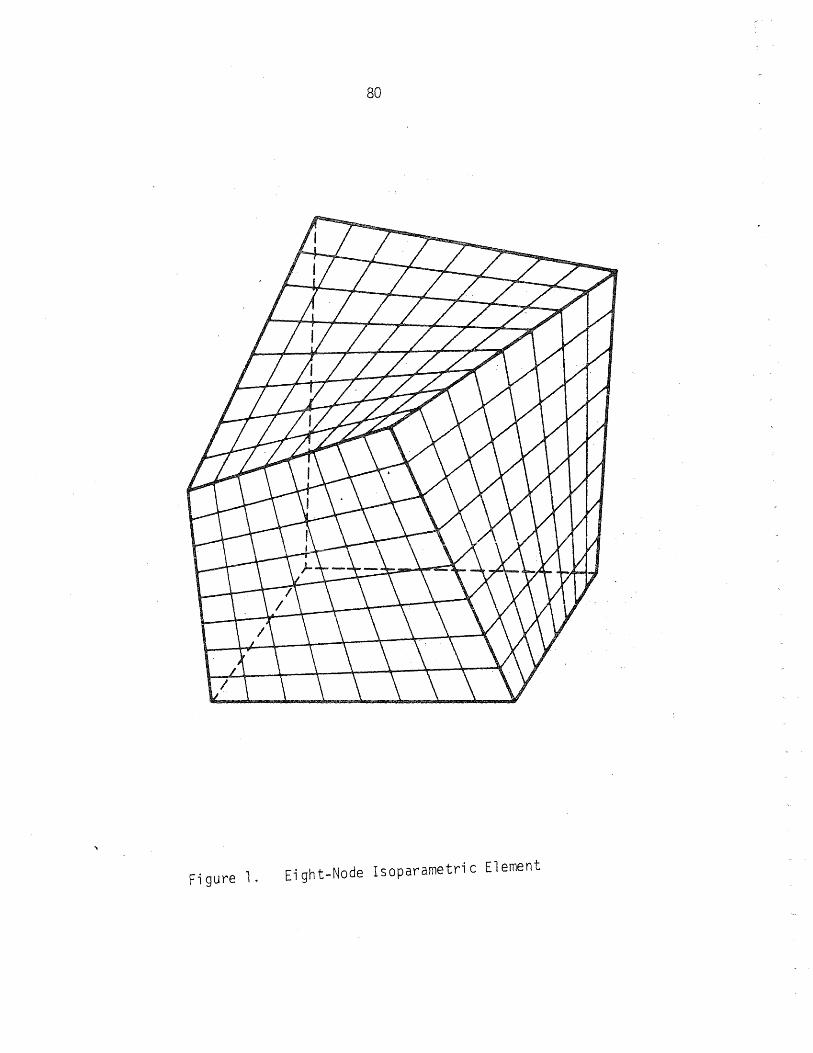
80
Figure 1. Eight-Node Isoparametric Element

.... J:!
" ....
~ I , I I
.... d.. ___ ...,o.
(a) 20-Node
81
I "c:t"--
"D'"
I , , ~ I ,
d'
(b) 32-Node
Fi gure 2. Hi gher Order Isoparametri c Elements
Fi gure 3.
'" .... .... '" '"
.... ,.,
, ~ , I I I
p..
A Mi xed I soparametri c El ement

<;2 " :1:/, <;3 " :1:/
A B ~1
(d) Linear A B
(b) QUddra ti c
~1
I AL------------ B .,~" ,
I
\ CD
/ \ c, f'\)
(c) Cubi c
A L ____ \-------.l B
. 3
. ... ""'"
(d) 1 + 7
Degree
F1 gUre 4.
A TYPlca / Edge AB Under Va .
rY7
ng Degree Of ResPonses

t ul b = - ul
t b u2 = -u2 t b u = 3 -u 3
83
Boundary
Structure
Boundary Constraint Equati.on
TIl = U2 cot 8
(a) Inclined Boundary
Xl
/ Lateral Loads
/l~l~l
(b) Auxiliary Constraints for a Typical Plate
Figure 5. Two Types of Displacem~nt Constraints

84 C5
C5 Y
C5 = yield stress y 0" = effecti ve stress e G = 0 for C5 d e y y C5 = C5 for G C5 e y
E = E + E e p
Figure 6 .. Bilinear Stress-Strain Curve for Uniaxial Loading
Va. lJ
Fi gure 7.
, ,
Initial Yield Surface
, , , ,
New Yield Surface
Graphical Representation of the Initial Stress Method

F
~F
F Y
85
F y = yi e 1 d 1 oa d
Uy = yield displacement
U
Figure 8. Modified Newton-Raphson Approach for Elasto-Plastic Analysis Under Uniaxial Loading
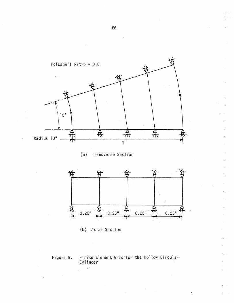
86
Poisson's Ratio = 0.0
Radius 1011 111
(a) Transverse Section
# 0.25" 1/IDo/~
0.25 11 0.25" ~
(b) Axial Section
Figure 9. Finite Element Grid for the Hollow Circular Cylinder

.J 8 q
o r q
11 .0
10.5
10.0
9.5
0.25
0.25 L 0.50
0.75
1 .0
87
0.50
x t
q
Present Study Theory of El as ti ci ty
Solution 55
0.75 1 .0
Figure 10. Distribution of Radial and Circumferential Stresses in an Infinitely Long Hollow Cjrcular Cylinder

Ew
88
208
Converged Value 207 • Ew = 207.15
E = modulus of e 1 as ti ci ty w = central deflection
206 • nxn = grid size
205
204
203
202
o 5 10 15 20 100
7
Figure 11'. Convergence Study on the Center Deflection of a Simply Supported Plate Under Uniformly Distributed Lateral Load
25

...
P/4 89
~0 ___ """"",_"""1111.4-
G
P = 40 1 bs
u1 = u = u = 0, 2 3 on EFGC ul
= 0 on OAEC Symmetry u = 0 2 on OBGC
(a) P ri s m
Xl ...........
tX3 Number of·elements = 64 Numb_er of j oi nts = 125 Number of unknowns = 260
(c) Finite Element Grid for the Pri sm
A ......................... ----.... ~ x2
C -----.
t . E
o
ul = u2 = u3 = 0, on COE
normal displacement = 0, on OAEC and OBOC
(b) Circular Cylindrical Segment
.,.,.,..""r ..... ...... .....
- .-- -- -.... ......
-
-....r .....
~X3- Number of elements = 12 . Number of j oi nts = 65
Number of unknowns = 112
(b) Finite Element Grid for the Cyli nder
xl -.-.
Figure 12. Finite Element Idealization of the Bouss i nesq Prob 1 em

'r-l/)
0.
'" l/)
l/)
OJ S-
+-> tI1
r--ro u
'r-+-> S-OJ >
6.0
4.0
2.0
0.0 0.0
k nL v.v
4.0
2.0
90
• Prism Idealization I Cy 1 i n de r I de a 1i z a ti on
.................... Ana lyti ca 1 55
2.0
0.0
A· ------------ A : I ,... - - - - -. - - - - - ~B C ----------- C o ----------- 0
E 1.----------- E
1 .0 . 3.0 4.0 5.0 0.0 1 .0 2.0 3.0 4.0
4.0 [. \ --
\ 2.ol~ , I '-
0.01 !~ i . 0.0 1 .0 2.0 3.0 4.0
2.0
Sec. x3
AA 0.625
BB 1 .25
CC 1 .875
DO 2.5
EE 3.75
5.0 6.0
.. 5.0 6.0
o. O. 0 L........_.J......_-L.._~...;......~~~ ... --'
0.0 1.0 2.0 3.0 4.0 5.0 0.0 1.0 ·2.0 3.0 4.0 5.0 6.0
Horizontal Distance from the Axis of the Load, in.
Figure 13. Distribution of Vertical Stresses in the Boussinesq P ro b 1 em 0 f a Semi - I n fi nit e Body Sub j e c te d to a 40 - 1 b Concentrated Load

7211
E ;:: 3 x 10⁶ ps i
v = 0
6 11
6 11
4211
(a) Axial Section
500 psi
91
u_ = 0 -j
Number of elements = 52 Number of joints = 172 Number of unknowns = 417
(b) Finite Element Grid
Figure 14. Axisymmetric Pressure Vessel
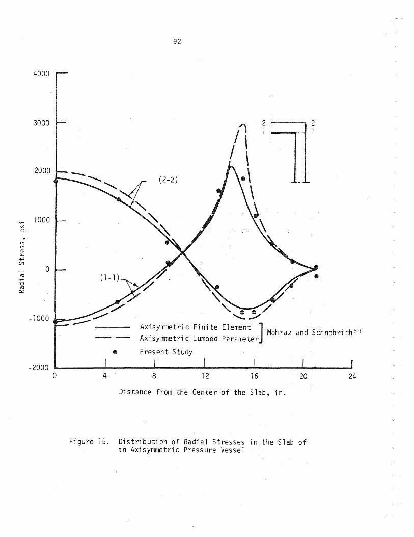
"r-Vl 0...
'" Vl Vl QJ s...
+-> V)
....-co
-a co
0::
92
4000
3000
" 2 2
/ I 1 1
/ \ 2000 .\ (2-2)
\ l 1000 ~
0
-1000 ~ __
-2000 o
Axisymmetric Finite Element ] Mohraz and Schnobrich 59
Axisymmetric Lumped Parameter
Present Study
4 8 12 16 20
Distance from the Center of the Slab, in.
Figure 15. Distribution of Radial Stresses in the Slab of an Axisyntnetri.c Pressure Vessel
24

V')
CL
...
3000
2000
~ 1000 QJ s....
+-> U)
'r-+-> c
~ 0 CJ 4-E :::l
·u s....
.u
-1000
-2000 o
93
(2-2)
- Ax; syrrmetr; c F; n; te} Element Mohraz and
-- Ax;syrrmetric Lumped Schnobrich 59 Parameter
• Present Study
4 8 12 16 20
Distance from the Center of the Slab, in.
Figure l6~ .Distribution of Circumferential Stresses in the Slab of an Axisymmetric Pressure Vessel
2 1
24
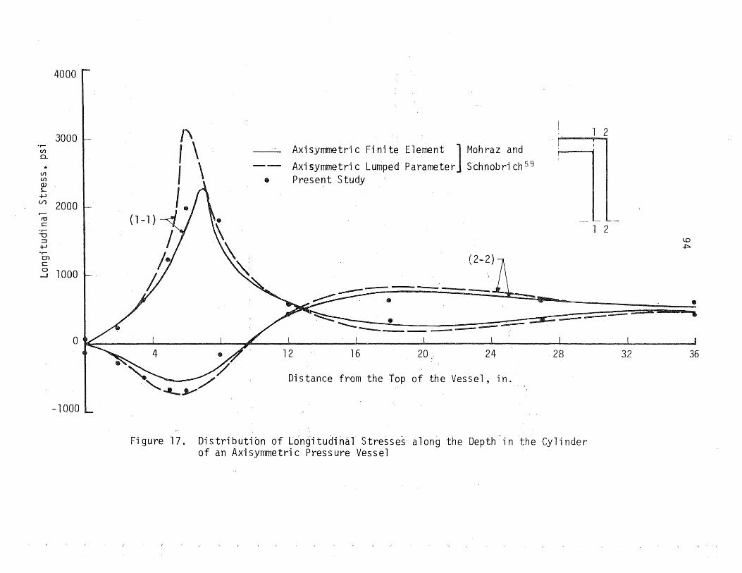
4000
i 3000 r /\ I \
~ 2000 ~ I \ I.
(1- 1 ) .r--0 ::l
+-> m t:
~ 1000
-- Axisymmetric Finite Element ] Mohraz and Axisymmetric Lumped Parameter Schnobrich 59
.. Present Study
~
---~
2
2
..-----
\.D +:>.
..
a k" /1 !
-1000
"12 16 20 24 28 32 36
Distance from the Top of the Vessel, in.
Figure 17. Distributibn of lon~ituaih~l Stresse~ al~ngthe Depth-in 'the Cylinder of an Axisymmetric Pressure Vessel

1011
95
Longitudinal Prestressing 26,000 psi
40" 3000 ps i
u3
;:: 0
(a) Axial Section at OA
E ;:: 4 x 10⁶ ps i \l;:: 0.15
Displacements normal to and OB ;:: 0
(b) Transverse Section at 1-1
Radi a 1 P restres sing 1200' psi
;
B
Figure 18. Prestressed Rea~tor Vessel with Cirdular Openings

H
o
A
(b) Enlarged View of El ement e
96
Number of elements = 48: Nurroer of joints = 173 Number of unknowns = 404
(a).' Pie~Sh~ped Axial Segment with the Finite Element Grid
Figure 19. Finite Element Grid for the Prestressed Reactor Vessel with Circular Openings_.

97
600
Openi ng Juncti on J ~ ~
400 2 "2
(2- 2)
2000 \ \
or-
\ (/)
0-
... 0 I (/)
(/)
<JJ s...
J +J V)
r-
J (ij or--a (ij
-2000 / 0:::
/ Di s tri buti on on the edge without opening
edge" wi th --- Di s tri buti on on the opening
-400
o 4 8 12 , 16 20
Distance from the Center of the Slab, in."
Figure 20. Distribution of Radial Stresses in the Slab of the Prestressed Reactor Vessel with Openings

6000
4000
'r-(/')
CL
" (/') 2000 (/')
ClJ s-
+J (/)
,..--(ij
'r-+J
s:::::: ClJ 0 s-ClJ 4-E ~ u s-
'r-U
-2000
-4000
0
98
Opening
/~ "-'~
2 I
-----~ (2-2) ,
/' I / Di s tri buti on on
I without opening
( 1- 1 ) I Di s tri buti on on wi th openi ng
/ I
/ 4 8 12 16
Distance from the Center of the Sl.ab" 'i n .,
Fi gure 21. Di s tri buti on of Ci rcumferenti a 1 Stresses in the Slab of the Prestressed Reactor Vessel with Circular Openings
2
the edge
the edge
20
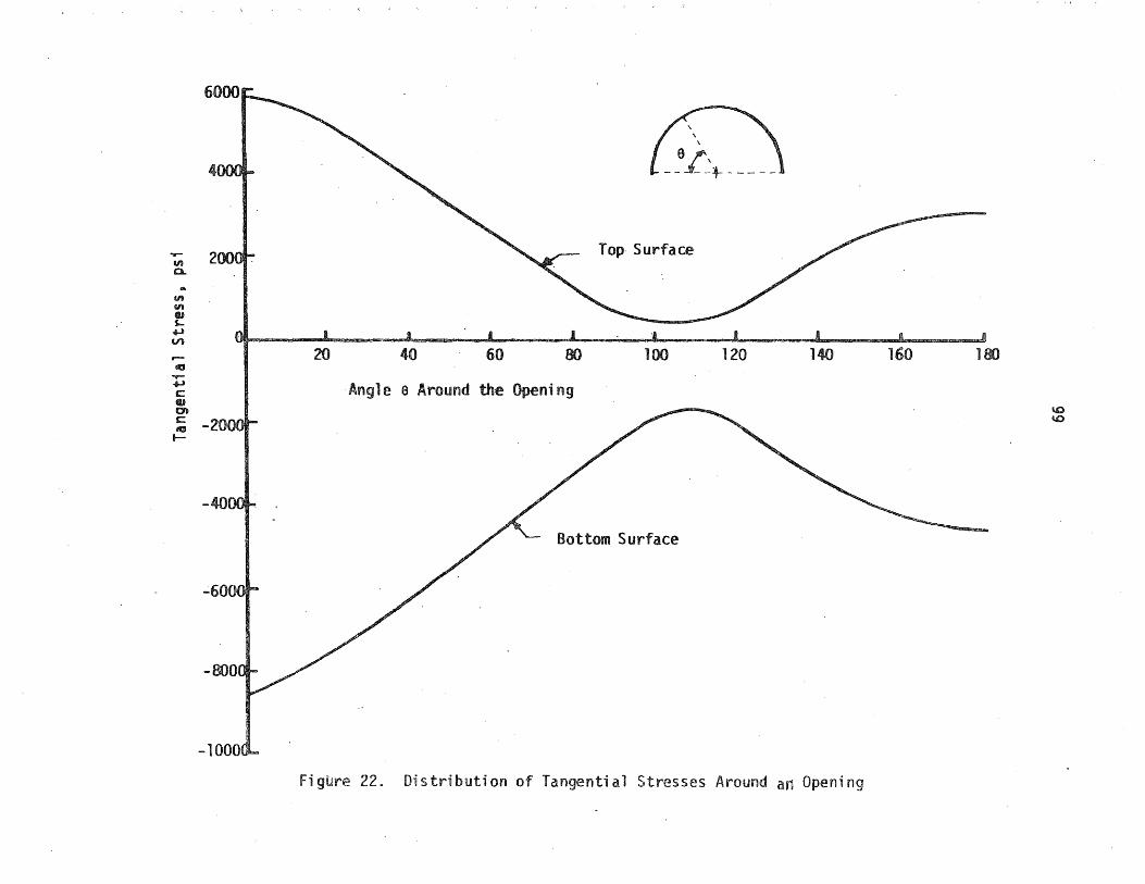
..II» 0...
en 111'8 cu S+l V)
110 .r-+l c: cu C1) c: AU I-
4 e JI'\ .Ji_ - l- - - - - -
Top Surface
40 60 80 100 120 140
I\n91 e a Around the Openi n9
Bottom Surface
Fig~re 22. Distribution of Tangential Stresses Around an Opening
160 180
\0
'"

100
2.0
1 .5
q = ; nterna 1 pressure
1 . a qy = q at the initiation of
q/qy yielding
u = radial displacement at the inside surface
u = u at the i ni ti a ti on of y yielding 0.5
Finite Difference
It Pres ent Study
0.0 --------------~----------------------------~------------~
0.0 1 .0 2.0 3.0
Figure 23. Load-Displacement Curve for the Thick Hollow Circular Cylinder Subjected to a Ut:1iform Internal Pressure
4.0

a a y
0.9
0.8
0.3
0.2
0.1
Fi gure 24.
101
Fi ni te ............................ Di fference 1
• Present Study
a
Ci rcumferenti a 1
Plastified Region
Critical Radius = 1.4 x a
1.4 1.6
r/a
a /a Z y Axial
The Distribution of Radial, Circumfe~ential and Axial Stresses in a Thick Hollow Circular Cylinde~ ~ubjected to Internal Pressure

0 -0 y
0.9
0.8
0.7
0.6
0.5
0.4
0.3
0.2
O. 1
a 10 8 Y
f"
102
a -1
.. o 10 r y
Radial
Fi ni te Di ffe,rence 1
Present Study
o.o~------~----~~~----~~--~~----~
1 .0 1 .2 1 .4 1 .6 1 .8 2.0
Figure 25. Variation of Radial and Circumferential Stresses at ria = 1.4 for an Increasing Internal Pressure

103
Beam 32"
Theoretically Plastified Region Plastified Nodes and Element Centroi ds (Present Study) . Nodes and Element Centroids in the Theoretically Plastified Region, whicH did not Plastify Numerically Intermediate Node
A T I o . , T I I I ,
. ,
~ I ~ ~ ~ ~ ~ ~ . -- ..... """ "'VI' .... .... '"'" C B
(b) Plastified Region.at q = 1.22 qy
o
B
(c) Plastified Region at q = 1.32 qy
A '0
C B
(d) Plastified Region at q = 1.36 qy
q = Lateral load on the beam qy = q at the initiation of yield
Figure 26. Comparison of Plastified Regions in a Simply Supported Beam at Three Different Load Levels

Cf.. I 104
,.......-r---r----,.-.,....-.....,.-........,..-.,-.,....-......,.-.......,...---r-..,..............,-......,...-~. - - - N e u t r a 1 Ax i s
One-fourth of the Beam with the Finite Element Grid
° y ° y 0y aGy
Stress Oi s tri buti on: 1. Beginning of th~ load increment
2.
3.
A 0y a0y
=
=
After elastic analysis for the load increment After subtracting the initial stresses
Stress loss Uniaxial yield stress
Elastic stress increment
Figure 27. The "Loss" of Stresses Due to Interpolation

1 .6
1 .2
L 0.8 qy
0.4
0.0
0.0
,q = qy
0.4 0.8
I, I ,
W = W
/
Y
/ /
/
/ / r- - = -~.:II-------------
•
q
qy
W
W y
A Plausible Elasto-Plastic Curve
Ideal Hinge Curve
Present Study
lateral load on the beam
q at the initiation of yielding
central deflection
W at the initiation of yielding
I " L____ _ ___ J ______________ ~L _____ , __
1.2 1.6 l.8 2.0
W/Wy
Figure 28. Load-Displacement Curve for the Beam
C)
Ul

-t--
i n ~
I
i
-t-
106
I ........... ----------------- - 10 i n ~ ______ . __ . ____________ ----+
I ----i-------~----t_--- --;----+-------
I ---+----r---+--~
I Fixed l Support
-----~------ -:------ +-----+---- t ------+---+---f-"--- I u =u =u =0 ! 1 2 3
(a) Axial Section of the Plate
I ntermedi ate Node
Poisson's Ratio = 0.24 Strain Hardening Coefficient = 0
I I I
J I \ i I I I I I
~---I- -- ----------+---- L ____ +-- ---L--i-----L--t---_-
I • ; i
• I' I i i ; I ---- I I --t-----t---.--+_ ---r------I----t
I I . I I I
--+---L--f---4----+----l
I
--:----+---_: ---+-
I
(b) Plastified Region at q = 1.3 qy
+-___ i __ --t---_l-_____ -+--- +-__ L_-+-_-I I
: I ! I· ---t-----L----t----i----+---L---+---t---~-
I' ; : I
: iii I , : I
---+------- - --L.------\--------1"------ - --- t------t---+--i---t-----: I I I
(c)
I I I , Plastified Region a~ q = 1.5 qy
Plastified Node or Element Centroid
Plastified Region
Figure 29. Elasto-Plastic Analysis of the Circular Plate

2.0
1 .5
1 .0
0.5
0.0 0.5
107
Present Study
Popov and Khojasteh-Bakht 13
El as ti c Curve
q =
qy =
w =
Wy =
1 .0 1 .5
----...---
uniformly distributed load q at the initiation of yielding
central defl ecti on w at the initiation of yielding
2.0 2.5
Figure 30. Load-Displacement Curve for the Elasto-Plastic C i r c u 1 a r P 1 a te
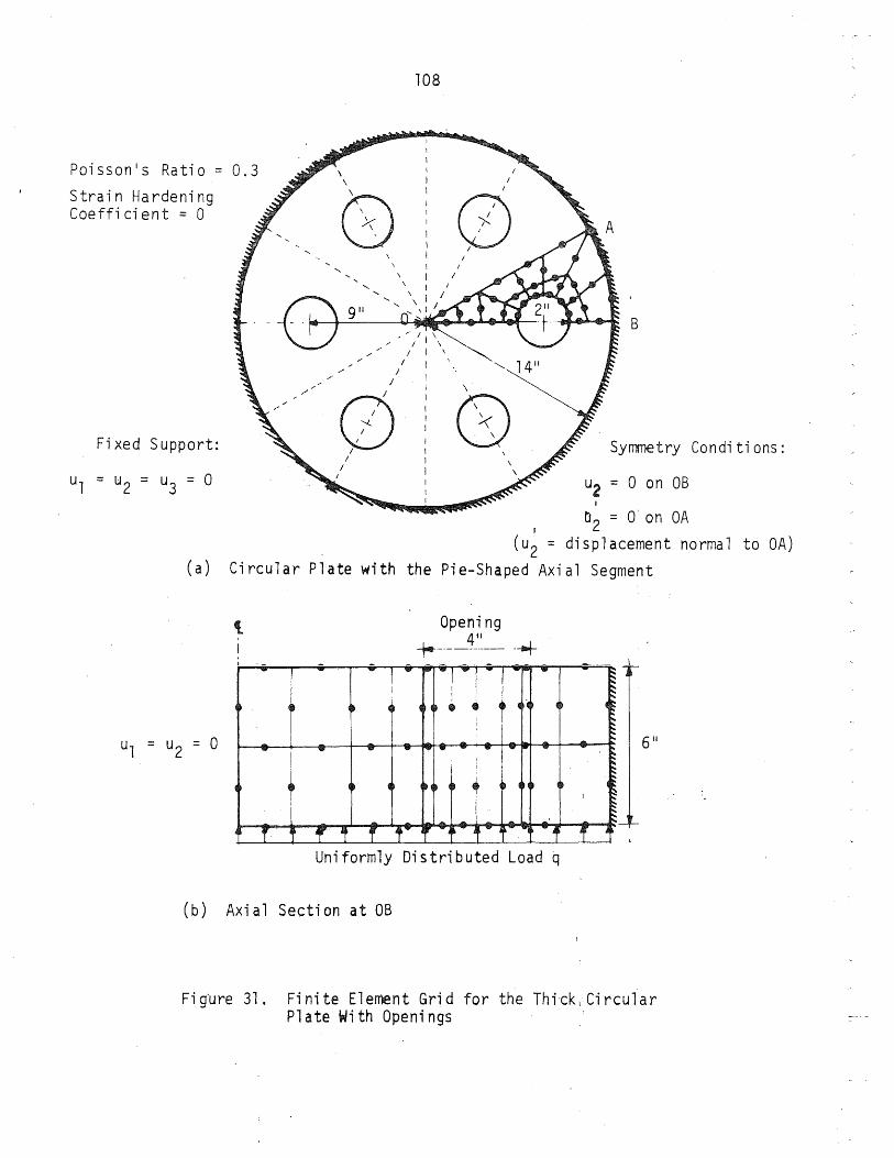
Poisson's Ratio = 0.3 Strain Hardening Coefficient = 0
Fi xed Support:
\ \
(0
(7) ):-/ I
/
108
/ I
/
o I
I
/
\
Q
B
Symmetry Conditions:
ul = u2 = u3 = 0 u2 = 0 on OB ,
I D2 = 0 on OA (u2 = displacement normal to OA)
(a) Circular Plate with the Pie-Shaped Axial Segment
; - - ;; - ....
p ~ ~
AI>. ... - "" ...
4 4~ C
-j 'f, lip ,. -r f ,-
Opening 411 -t-.---- .. --- ---+
~-I-I-r-..,
, .• ~ t '" 4.
I I ... ""!' ...
! ... 1- .. j
~ ~ • • ~ ~, ~
L... Ao. I '" IF' ~ , '" I' -1
Uniformly Distributed Load q
(b) Axial Section at OB
..,~ ~ .p
~ I
~
~
..... ~ 6"
I
Ir
f j
,
Fig'ure 31. Finite Element Grid for the Thi'ck , Circular Plate With Openings

109
2 [---------@--- --j : :E--·~: . 3 3 Section OA Section OA
f~------f-tl---j : . :F~--l~-J: 2
3 Section OB Section OB
.0 ___ ----11l&1li
0 ........... .&&&111...-- ---B
Section 1-1 Section 1-1
0 ___ ----' '----__ B 0 ___ _ '---__ B
Section 2-2 Secti on 2- 2 :.
A A
o "'----IllS 0----Section 3-3 Secti on 3-3
(a) 1.75 x Yield Load (b) 1.95 x Yield Load
• Pl as tifi ed Reg; on
Fi gure 32. Pl as ti fi ed Regi ons in the Ci rcul ar Pl ate wi th Circular Openings at Two Load Levels

APPENDIX A
COMPUTATION OF· THE NUMERICALLY· INTEGRATED, STI FFNESS' MATRIX
AD 1 General
It was indicated in Chapter 2 that the closed form integration
for the evaluation of the stiffness matrix of an isoparametric element'is
a prohibitive task. In such cases, a numerical integration scheme is
employed. Although.numerical integration for the evaluation of the
element'stiffness matrix'isboth simple and adaptable to computer'pro
gramming, it increases thecomputations.to·beperformedsignificantly.
The increase in computations presents an.economic.disadvantage, espec
ially for large three-dimensional problems .. For this.reason,it is impor-
. tant to employ. effi ci ent schemes. fot.. reduci ng the. numb~r. of computati ons
wi thi n the. computer. 62
. It was, found during the course. of this·.study that the formula
tionof the element stiffness matrix in·index notation. results in a
better organization of computations .. A method. of computation is pre-
.. sentedin the.following.section .. ·Later a comparison.between the proposed
.. method andthe~conventional~method.of computation.is:made.in order to
ascertain their.relative,efficiencies.
A~2. Computational·Procedure
In. general , the element stiffness matrix can be.evaluated.by
. numerically integrating.Eq. 2~45.or.Eq. 2~42·for:isotropicand aniso
tropic'material properties, . respectively. Since.each.set of.computation
, is. repeated at every. poi nt. of i ntegrati on' in the' e 1 ement, one can. reduce
the number··.of operations significantlY.by taking the terms which are
not functions.of the.position coordinates outside.of theintegral·.sign
110

1'11
when possible. For homogeneous materials, the.elementsof.the material
. property. tensor Eijk£.are not functions.of the position coordinates~ .In
such cases, an integration ar'ray wTj which is given by
w~~ = JaNmdNn
dV (A.l) lJ axo ax" .
v 1 J
is first evaluated. The result is then multiplied by the material pro-
perty tensor' to give the desired element stiffness matrix .. For·an.iso-
tropic elastic material,
·kmon. = 'Wmeno + ('Wmn Wmn ) • II. 11 kk <5" e + e • . lJ1J· lJ Jl
and for an anisotropic elastic material
. mn mn ko .. = Eoke n Wkn .1J lJ.x.. N
(A.2)
. (A.3)
For nonhomogeneous.materials.theelements of the material prop
erty. tens or E c e k i'i are functi ons ,of the. pos i ti on coordi na tes .. Therefore, .1 J :AI
the material property. tensor cannot be takenoutside.of the integral sign
and it must be included in the integrationo ,For sUch cases the.number.of
operations for evaluat1ng.theelement·stiffness matrix is significantly
increased. However, as.is shown in the.next.section, the amount of com-
putation is still considerably less than that required.by the conventional
. procedure 0
A.3 Comparison. of Numerical : Computations
" In the.conventional .approach,.theformulation of the element
stiffness matrix is,given.by
·(A.4)

112
where
B = a.geometrymatrix.relating.strains to. displacements
o = materi a 1 . property rna tri x
For numeri ca 1 i ntegrati on the wei ght coeffi ci ent associ ated wi th eve,ry
point of integration is first multiplied into the material property
matrix. The'productBTOB'is then'evaluated at the integration points
through the element. The individual terms:are added to. give the elements
.of·the stiffness matrix. The steps and the number:of.operations (addi
tions and.multiplications) for evaluating the.stiffnessmatrixof a
. three-dimensional element:are given in Table A.l. If ~ and IT denote
the number. of, add; ti ons and mul ti p 1 i cati ons , : respecti ve ly, . one. obtai ns
(A.5)
IT l . = (27r2 +-117r+36)I
where
. r = number of nodes in the element
I = number of integration. points' in the element
In the. proposed. procedure for.the case in whichthe·elements.of
the mater; al . property tensor Ei jk,Q, are· not functi ons of. pos; ti on coord; n
ates (anisotropic material : property is considered. for generality), the
. wei ght coeffi ci ents . at every i ntegrati on. poi nt: through the element
are first multiplied_into the.derivatives.of~shape.functions .. The indi
vidual .terms.of.the integration.array W~~ are. then. added and. the. result .1 J
is multiplied.by the.elasticity tensor. to. give the elements .of the stiff-
ness matrix. The steps and the.number.of additions.and.multiplications
.. for a.three~dimensional.element·.are:given in Table A.2 .. Thus,

113
9, ). 2 ) L2 = 2 (I + 9 (r + r
(A.6)
IT2 = ~ (I + 9)(r2 + r) + 3rI
For isot'ropic elastic material where the material property tensor
can be expressed in terms of Lame I s cons tant and modul us of ri gi di ty,
.Eqo 2044, the number of operations can be somewhat. decreased. However,
the. decrease is not. very si gni fi cant.
A similar procedure for the evaluation.of.thestiffness matrix.in
whi ch the el ements of the materi a 1 property. tens or are fun cti ons . of pos i
tion coordinates {honhomogeneous material) is given in Table A.3. The
number.of additions.and multiplications for a three~dimensionalelement
.. are
2:3 = 18[r(r + l)J I + 81rI
.. (A. 7)
IT 3 . ~ 2~ [r(r + l)J I + 81(1 + r) I
In order to obtain a measure for the.amount.of computation. in
.volvedin various.procedures, a simple three-dimensional .element.(eight
nodes) and a.high order three-dimensional element with two.intermediate
nodes on eachsi de. (thi rty~two' nodes)-. are' consi dered o . In both. cases, . it
is assumed.that.fourth order Gaussian quadrature is used for.thenumertcal
integration (sfxty-four integration points in the element) o. Thenumber.of
additions and multiplications for various procedures .are given in Table
A.4o
The results.presented in Table A.4 indicate that the number of
.operations for the evaluation of the stiffness matrix.by the proposed

114
method is approximately one-sixth of that required by the conventional
procedure 0 The computational ratio (the ratio of the addition or the
multiplication in the proposed method to those of the conventional pro
cedure) does not change significantly' when the number of nodes in the
element is increased .. For cases in which the elements of the material
. property' tensor are' functi ons of pos i ti on cpordi nates ,. the computati ona 1
ratio is in order of 0.6, Table A.4, .resu1ting in a40 percent reduction
in the computational effort.
A plot.of the total computational. ratio (addition and multipli
. cation) .versus.the order of Gaussian.quadrature.integration for both the
ei ght node and the thi rty-two node el ements is. gi ven. in Fi g. A.l. For
the constant material properties,the ratio decreases as the order of
· .Gaussianquadrature.is increased .. The.tota1 computational ratio is larger
. than unity for only-the first order·.integration .. This indicates that for
such a case, where the integration is simply the. volume of the element,
no computational .savingis achieved.by the. proposed. procedure. However,
thefirst.order quadrature.is.seldom.used.for.integrationoThe fourth
· '. order. quadrature is' the one. us ually. recommended. for the. numeri ca" i nte
· .gratian of the.elementstiffness matrix. ~7
.' For. the vari ab 1 e. materi a 1 .. properti es, the. tota 1 . computati ona 1
.ratio.remains.constant.regard1ess.of the.orderof.integration. Although,
significantly more. computational .effort.isneeded for elements with vari
ab 1 e materi a 1 properti es, . the. number. of computati ons . is. s ti 11 . we 11 be low
that.of the conventional.procedure.
No extra.storage.is .needed.for the.evaluation.of the.integration
. array- W~~, . Eq. Ao 1, as it. uses. the. same. storage. space. as the' sti ffness .1 J

115
matrix krjo A 3 x 3 array is the only space needed for the calculations
contained in Eqso Ao2, Ao3o In addition, W~~ and K~~ can be stored in a .. 1 J 1 J
column array to avoid the unnecessary multiple indexing.
There are two factors which contribute to reduction in the number
of computations in the proposed methodo One is the organization of the
formulation which is easily achieved by the index notation .. The other is
the real i zati on tha t the materi a 1 property tensor can be mul ti p 1 i ed out
side.of the integral sign for cases in which the terms. in the material
. property tens or a re not fun cti ons 0 f. pos i ti on coordi nates.

Tab 1 e A. 1
Operati ons Requi red. for the Eva luati on. of the' E1 ement Sti ffness Matri x Three-Dimensional Element.(Conventiona1 Procedure)
Computation Step
1. For each point of integration
a. Product of weight coefficients and material property matrix 0
b. Obtaining the product DB
c. Obtaining BTDB(upper triangular portion only)
Total for step 1
2. Repeating the.operations in step 1 for I integration points
3. Summing up the individual elements of the.stiffness matrix evaluated at I integration points
4. Total number of operations to obtain the element stiffness matrix (steps 2 and 3)
r = number of nodes in the element
Number of Additions
6 x 6 x 3r
~[6 x 3r(3r + 1)]
27r2 + l17r"
(27r2 + l17r)1
~[3r(3r + 1)J1
1(63r2 + 237r)I
I = number of integration points in the element
Number of Mul ti P 1 i cati ons
6 x 6
6 x 6 x 3r
~[6 x 3r(3r + l)J
27r2 + 117r + 36
(27r2 + l17r + 36)1
(27r2 + 117r + 36)I
---J
(J)
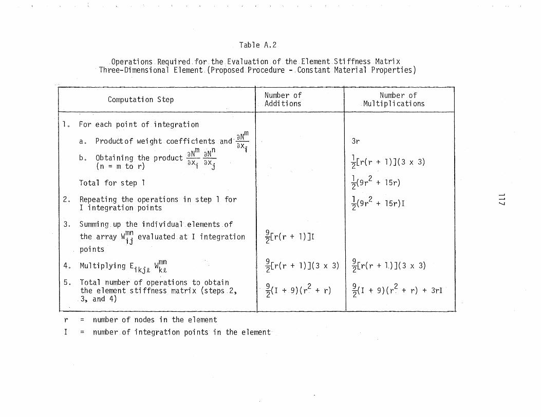
Table A.2
.Operations.Required.for theEvaluationof.the.Element.Stiffness.Matrix Three-Dimensional E1ement.(Pro~osedProcedure -.Constant Material Properties)
Computation Step
10 For each point of integration m
a. Product of wei ght coeff; ci ents and' ~~o m n 1
b. Obtai ni ng the product ~~:- ~~ c
(n = m to r) 1 J
Total for step 1
2. Repeating the operations in step 1 for I integration points
3. Summing.up the individual elements.of the array W~~ evaluated.at I integration
lJ
4.
points mn
Multiplying Eikj~ Wk~
5. Total number of operations to obtain the element sti ffness matri x (steps. 2, 3, and 4)
r = number of nodes in the element
Number of Additions
9 2[r(r +l)JI
9 2[r(r + 1)J(3 x 3)
9 2 ~(I + 9)(r. + r)
I = number of integration points in the element
3r
Number of .Multiplications
~[r(r + 1)J(3 x 3)
1 2 2(9r + 15r)
1 2 2(9r + 15r) I
9 2[r(r + 1.)J(3 x 3)
~(I + 9)(r2 + r) + 3rI
--i
......

Table A.3
Operations Requtredfor the Evaluation'of the Element Stiffness Matrix Three-Dimensional Element {Proposed Procedure ~ Variable Material Properties)
Computation Step
1. For each point of i~tegr~tion "
a. Product.of weight- coefficients and Eijki
. . . aNm b. . Obtal nl ng the. product E; kj Q, aX
k c. Obt~i~ing the product
m, n E . dN. aN ( t) i kj Q, ax ax n = m 0 r
k i
Total for step 1
2. Repeating the operations in step 1 for I integration points
3. Summing up the individual elements of the stiffness matrixevaluated.at I integration points
40 Total number of, operations to obtain the element stiffness matrix (steps 2 and 3)
r = number of nodes in the element
Number of .Additions
B1 r
~[r('r + 1)J(3)
2~ [ r (r + 1) J + Bl1 r
B1
Number. of Mu1 ti P 1 i cati ons
B1r
~[ r (r + 1) J ( 3 )
2~[r(r + l)J + B1(1 + r)
2 ~ [ r (r + 1) J I + IB1 r I 12 ~ [ r (r + 1) J I + B1 (1 + r) I
9 2[r(r + l)J1
1B[r(r + 1)J1 + IBlr1 12~[r(r + l)J1 + B1(1 + r)1
I = number of integration points in the element
co

Table A.4
Comparison of Computations.for.Determination.of Element.Stiffness.Matrix .(Three~DimensionalElement with 64 Integration Points)
8.nodes. 32 n.odes Procedure . Addi ti on .Multip1ication Addition . Multiplication
Conventi ona 1 189,696 172,800 2,307,072 2,011 ,392
Proposed Constant Eijkt 23,652 25, 188 346,896 353,040
% Con venti ona 1 13 15 15 18
Proposed I
Va ri ab 1 e E .. k Q, . , J 124,416 108,864 1,382,400 1,083,456
% Conventi'ona 1 .66 63 60 54
----.- 1-. _____ ~ ~ ------ -------- - -.-.--.-~
---II
~
~

120
8-Node Element 1 .2
o 1 .0 +.J rt5
(:;,."-"
'r-+.J n:l
+.J ::::'5 0... E o
u
0 'r-+-' ro
0::::
r-ro s::::: 0
'r-+-' ro +-' ::::'5 0... E 0
u
r-ro +-' 0 I-
0.8 Variable Material Properties
0.6
0.4 Constant Material Properties
0.2
O~--------~--------~----------~--------~--------~
\
1 .2
1 .0
0.8
0.6
0.4
0.2
0
1 2 3 4 5
32-Node Element
Variable Material Properties
Constant Material Properties
1 2 3 4 5
Order of Gaussian Quadrature Integration
Figure A.l Relationship Between Computational Ratio and Order of Gaussian Quadrature Integration
6
6

Appendix B
THE ISOPARAMETRIC ELEMENT IN. CURVILINEAR COORDINATES
Bol General
The isoparametricelement, as presented in Chapter2,has.been
formulated in a cartesian coordinate.system.The curved surfacesare.ideal-
i zed. by . defi ni ng' intermediate nodes. on . appropri ate' edges Q •• Intermedi ate nodes
are also used.if a higher order displacement.field is.desired .. If a.curvi
linear coordinate. system which defines the.geometry.of thestructurecan.be
· . sel ected, .. one. need. not. use i ntermedi ate. nodes.for. defi ni ng the. geometry. of
· .. the. structure ... For examp 1 e, .' for, cyl i ndrrica 1: type structures., ,one. can avo; d
intermedi ate .nodes .by. using a. cylindrical. coordinate. system ... Simi·larly,
· ,spherical coordinates may.be.employed.for.sphere.type· structures ..
B02 .. StiffnessMatrix
In curvilinear coordinates,.the.strain.tenior E ••. is.defined.as .. , J
. E· •. ~. 21. (u. I. + UOI') .,'J. lJ .Jl
(B.l )
where Uti j represents the covari ant. der; vati ve .of ui with. respect to xj .
. It is implied that x .. represents the curvilinear.system.ofcoordinates .. J
under.consideration. The.covariant.derivative.ui 1j·is.obtained.from
. au. :=:' -' -' + R .. k uk .dX~ .1J
.J
in whi ch Ro. k denotes the. Chri s toffe 1 , symbol. of. the. secoh.d ki nd. 6 3 .1 J
.. Eq ua ti ons . B. 1 , B~ 2 and' 2.2. yi el d
. E •• . . 1 J
121
(B.2)
(B.3)
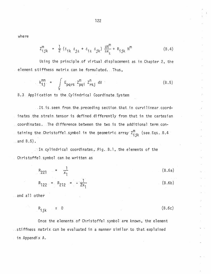
122
where
m 1 aNm Z,ok = 2(o'k o 'n+ o on OOk)-,\-+R"k Nm
1 J 1 J N 1 N J aX£ 1 J (B. 4)
Using theprinciple.of virtual .displacementas.in Chapter.2, the
element stiffness matrix. can be formulated ... Thus,
k~~. = J [ . Zm , Zn . dV . 1 J . P q rs . . pq 1 rs J
(B.5) v
B.3 Application to the.Cy1indrical . Coordinate. System
It.is.seen. from.the.preceding.section that.in.curvi1inear.coord
inates.the.strain.tensor isdeffneddi~ferently from that in.the cartesian
coordi na tes ... The di fference. between. the. two. is. the addi ti ona 1 . term. con
taining theChristoffel .. syrnbol.in the.geometric arraY'Z~ok (see.Eqs.B.4· .1 J
.and B.5).
In. cyl i ndri ca 1 coordi nates ;. Fi g. B. 1 , . the. elements of the
Christoffel . symbol can be.written as
R = 1 .. 221 xl
~122 R212 · ... r = = -2X1
and all other
R. ok - 0 lJ
(B.6a)
(B.6b)
(B.6c)
Once the elements .of Christoffel. symbol. are. known, the element
.stiffness matrix. can be evaluated in a manner simi1ar.to.that.explained
in.Appendix A.

123
B.4 Numeric&l' Result
Ah axisymmetric pressur~vessel ,.identical to the one analyzed
in Section 4.2.5 is solved in.cylindrical coordinates .. A similar grid
spacing as the one in Section 4.2.5.is.used,.Fig .. 14. Since intermediate
nodes in the circumferential' direction are not. required. for conforming to
the. cyl i ndri ca 1 boundari es, they are omi tted. The. n umeri ca 1 . res ul ts ob
tained.using the.cylindrical coordinates are identical .to those obtained,
using cartesian coordinates, Figs.' 15 - 17 .
. 8.5 Di s cuss ion
It may be advantageous to use the isoparametric elementincurvi
linear coordinates.because it would. largely eliminate.the.necessitY.of
introducingintermediate.nodes.for conforming. to the. curved boundaries.
This will,. in. turn, decrease. the total . number of unknown displacements.
There are two.factors.which may limit. the usefulness of employ
ing curvilinear coordinates ... It.can be shown that, in general, .thedis-
. placement. fi e 1 din. curvi 1 i near coordi nates. does. not sat; s fy the condi ti on
.of rigid.body.motion nor does it.provide.for constant straino Therefore,
a great. deal of care must.be taken to use the.element only fo~ cases in
which the error due to the violation.of the above mentioned conditions is
negligible or minimized. Another drawback of the curvilinear isoparametric
element is that the expression for the element stiffness matrix, Eqo 8.5,
is relatively complex. This will tend to increase the number of computa
tions in evaluating the stiffness. matrix. On the other hand, since the
. decrease in the number of unknown displacements reduces the computational
.. effort required. for solving the equations, it is.possible that for certain

124
.problems the use of. the curvilinear isoparametric~elementresults in sub
stantialsaving in. the' computer time.

A
I I I
125
-------,---...... ".",. .............
,/ I " / "
/1 I I
o
Figure B.l Cylindrical Coordinates
3
B

.AppendixC
.TRANSCENDENTAL SHAPE FUNCTIONS
Col General
In the formul ati on of the isoparametri c element, generally poly-
namia1 shape functions have been used. The use of. polynomial shape.func
tions assures the existence of the rigid body motion and the state of con
stant strain. in the displacement field,.Section 2.3. For higher order
elements, .Section 205, the displacement field is considered as consisting
of two. parts, ali nea r di sp 1 acement fi e 1 d as . defi ned. by the corner nodes,
and the depa rture from the 1 i near fi el d on i ndi vi dua 1 edges. as . defi ned. by
intermediate nodeso .In this case, conditions.of rigid body motion and
constant strain are satisifed.by using.polynomial shape. functions for the
corner nodes alone, regardless of the variation,of the departure from
linearityas.defined.by the intermediate nodes. This means that one has
freedom in theselection.of the shape functions for the intermediate
nodes e Po lynomi a 1 functi ons are one possi bi 1 i ty and· have. been a 1 ready
employed. Another possibility is the use.of transcendental shape. functions
This selection is.developed in the following section.
Co2 Development.of the.TranscendentalShape. Functions
An individual edgeAB.of an element, Fig. 4d, with I intermediate
nodes is considered. As in Chapter 2, let ~denote a component.of coordin
ates or displacements. The value of ~ on the edge AB is denoted by ¢ABo
The variation of ¢AB along the edge is defined.by.Eqo 2.16. The.term ~AB~
denotes the departure of ~AB from the linear variation defined by the cor-
ner nodes A and Bo In general, one can write
126

where
/jAB¢ _ s' s 'y g
127
s y = a set of I unknown coeffi ci ents, and
(C.1 )
gS = I functions of the isoparametric coordinates along the
edge AS, ~1 in this case.
The right-hand sidenf the,Eq. C.l can,be looked,uponas a trun-. .
cated serieso A polynomial series which resulted in polynomial shape, func-
tions was used in Chapter 2. Other series expansions may also,be used.
A Fourier series expansion, due to i tsrapi d convergence. property , is con
sidered,hereo .Again,as in Chapter 2, each of the individualfunctionsgS
should satisfy the constraints imposed, upon ,6 AS <p , namely they should
vanish at the corner nodes A and,S (~l = ±l). The sth terfuofthe, FoDrier'
series which satisfy this constraint is given,by
Once the functions gS have been defined, the steps used 1n Eqs. 2.26 -
2031 can be followed in o'rder to obtain the shape functions and the modi
fiednodal values,of <po
C03 Numerical Result
A sfmpleproblem has been solved in order to, demonstrate the use
of transcendental shape functions. A thick hollow circular,cylinder (inter
nal and external radii of 10 in. and 20 ino, respectively) subjected to a
uniform internal pressure is analyzed. Due to.symmetry, a pie-shapedseg
,ment is considered and is divided into 5 elements with intermediate nodes
in the radial and circumferential directions. The distributions.of the
128
radial and circumferential stressesobtained.by the present method and
those obtained by the theory of elastiti cy55 are given in Fig. C.l. As
can be seen, the agreement between the two is excellent.
C.4 Discussion
The application of transcendental shape functions in isopara
metric element has been demonstrated. Its relative efficiency as compared
to polynomial shape functions is a matter requiring more detailed investi
gation.
For a two-dimensional rectangular element with one intermediate
node on each edge, the traces of the two element s ti ffness matri ces ob
tainedby using the. polynomial' and transcendental shape functions,' respec
tively,.were computed, and are in ratio.of 1.273:1.0. This comparison, .
a 1 though. 1 i mi ted to two-dimens i ona 1 rectangul ar elements, i ndi cates that
the trans cendenta 1 shape functi ons a 11 ow the element to be more fl exi b 1 e.

1 .2
1 .0
° q"
0.8
0.6
0.4
0.2
o o 0..2 0.4
° /0 r '
129
1011 t = 10"
0 e/q Ci rcumfe renti a 1
Theory of Elasticity Solution 55
Present Study--Using Transcendental Shape Functions
Radial
0.6 0.8 1 .0 x t
Figure C.l Distribution of Radial and Circumferential Stresses "in" a Thick Hollow Circular Cylinder

130
LIST OF REFERENCES
1. Hodge, Po G. and White, Go N., "A Quantitative Comparison of Flow and Deformation Theories of Plasticity," J" Appl. Mech., Vol. 17~ 1950 , P p. 1 80 - 1 84 . .
2. Koiter, W< Tes "On Partially Plastic Thick-Walled Tubes," Biezeno Anniversary Volume in Applied Mechanics, N. V. De Technische Uitgeverij H, Starn, Haarlem, 1953, pp. 232-251.
30 llyshin, A. Ao, "Some Problems in the Theory of Plastic Deformation,1I RMB-12, Transaltion from Prikle Math. Mech., Vol. 7, 1943, pp. 245-272, by GradQ Div. Appl. Math., Brown University, 1946.
4. Mendelson, A~ and Manson, S.S., "Practical Solution of Plastic Deformation Problems 1n Elastic-Plastic Range," NASA, Technical Report R~28, 19590
5. Mendelson, A. and Spero, S. W., "A General Solution for the Elastoplasti c Thermal Stresses in a Strain' Hardenin~ P'late with' Arbitrary Material Properties," J. Appl. Mech., Vol. 29,1962, pp. 151-158.
6. Davis, Eo A., "Extension of Iteration Method for Determining Strain Distribution to the Uniformly Stressed Plate with a Hole,',' J.Appl. Meche, Vol. 30, 1963"pp. 210-214; Discussions, ibid., Vol. 31, 1964, ,pp. 362-364. . --.
7. Tuba, I. S.,uElastic-PlasticStress and Strain Concentration Factors at a Circular' Hole in a' Uniformly Stressed Infinite' Platei" J.,Appl. Mech., Volo 32, 1965,pp.' 710-711.
8. Argyris, J. H., Kelsey, S. and Kamel, H. J "Matrix Methods .. of Str.uctural . Analysis--A.Precis of Recent.Developments," Matrix' Methods in'Structural' Analysis--AGARDograph 72, Ed., B. F. deVenbeke, Pergamon Press, Oxford" 1964.
90 Argyris, Jo H., "[lasto;..Plastic' Analysis.of Three Dimensional' Continua!!11 J. Royal' Aero. Soc., Vol. 69, 1965.
10 .. Swedlow, To L., Williams, M. L. and Yang, W. M., "Elasto-Plastic . Stresses in.Cracked.Plates,"· Ca1citReport SM' 65 ... 19, California Insti. tute of Technology,' 19650
11. Marcal, Po Vo and Pilgrim, W. R., "Stiffness.Method for Elastic-Plastic Shells.of Revolution," J. Strain'Analysis, Vol.,1,1966, p.·399.
12. Ueda, Y. and Matsuishi, Mq "Analysis of Elastic Plastic Buckli,ng of Plates,by the Finite Element Method," Proc., Japan-U.S. Seminar' on Matrix Methods in Structural' Analysis and' Design, Tokyo,· 1969.

. 131
1 3 0 Pop 0 v " E 0 Po, Kh 0 j e s te h - B a k h t, M" and Y a 9 h rna i, S., II A n a 1 ys i s 0 f Elastic-Plastic Circular Plates,1I J. Eng, Mech. Dive, ASCE, Vol a 93~ 19670
14. PopOV, Eo P q Khoj as teh-Bakht, M. and Yaghmai, S., JlBendi ng. of Ci r~ cul ar PI ates. of Harden; ng Mate'rial ," Int. J. Sol i ds Struct., Vol .. 3, 1967,pp. 975-988 0
15. Khojasteh-Bakht,·M., JlAnalysisofElastic":Plastic She11sof Revolution· Under Axisymmetric Loading," Ph.D.' Thesis, University of California,· Berkeley,· '1967.
16. Zienkiewicz, O.C., Valliappan, S. and King, I. P., "Stress Analysis . ·.of Rock as a !No Tension l Material,IIGeotechnique, Vol. 18, No.1, · 1968,pp. 56-660
17. Maier, G., ."AQuadratic Programming Approach for Certain-Nonlinear · Structural: Problems,1I Meccanica, Vol .. 3, .1968, p.121 •.
180 Maier, G., IIIncremental· Plastic Analysis: in: the:Presenceof· Large '. Displacements' and: Physical· Instabilizing·.Effects~II'. Int. J.Solids
.. Structo,Vol~· 7, 1971,~pp~345~372.
19. Lopez,L. A. and·Ang,AoH.-S.,I'Flexural Ana1ysis·.·ofElastic Plastic " Rectangul ar" PI ates, II Techni cal:' Report,: Department: of Ci vi" Eng; neeri ng, · Uni vers i ty,. of I :11 i noi s , Urbana, :.1966.
20 .. Shoeb',' N. Ao' and Schnobrich, W. C., JlAnalysis .of Elastic-Plastic Shell Structures, II Ci vi 1', Engi neeri ng',Studi es, Structural'" Research. Seri es
'Noo' 324,University,of Illinois, Urbana"1967.
21. Galloway, Jo Co and Ang;·A.·H . .,.So, JlAGeneralized:LumpedParameter Mode 1 for Pl ane,·Problems. of Sol i d Medi a, II. Ci vi 1 ' Engi neeri ng S tudi es , Structura1'.Research"Seri'es' Noo', 341 ,University-,of Illinois, Urbana,
· 196 8 ~
220 Mohraz, Bo, Schnobrich, W~ Co and Echeverria Gomez,' A., "Crack , Development, in a' Prestressed' Concrete: Reactor:Vesse 1 as, Determi ned '.by a Lumped': Parameter-, Method,II, Nuclear·'Engineering and Des;'gn,···Vol.· 11, ,1970"PPi 286-294. '
23. ,Zi enki ewi cz, O. Co and' Cheung" Y .' K., liThe Fi ni te E1 ement Method ',for Analysis ,of Elastic Isotropic and Orthotropic Slabs,"' Inst'. Civ. : Eng., Proco, Vola' 28, 1964,~pp~ 47J~488.
240 Argyris, J. H., liThe Lumina Elementfo'r the' Matrix Displacement· Method,1I , Aero~' J. Royal Aero,' Soco,' Vol 72, No. 690,'1968, p.' 514.
250 Argyris, 'J. H., F'ried,·I. andScharpf,·D.·W., liThe Hermes 8 Element for the Matrix Displacement Method, II Aero. J. Roya] , Aero. Soc. , Vol c 72, Noo' 691, 1968, p~ 613.

26.
27.
28.
29.
,30.
31 .
, , 32.
132
Martin, H. C., IIPlane Elasticity Problems and the Direct Stiffness Method,1I Trend in Engineering,' University of Washington, Seattle, Vol. 13, 1961.
Gall-agher,' R.H., P·adlog,J. and Bijlaard,P. P.,"StressAnalysis of Heated Compl ex Shapes, II, J. Am. Ro~ket Soc. , 1962, p. - 700.
Argyris, J. H., "Three Dimensional' Anisotropic and'Inhomogeneous Elastic Media~ Matrix Analysis for Small and Large Displacements," Proc~, 11th'Int. Cong~ ,Appl. Mech., Munich, 1964.
Argyri s, J. H., 11Th ree Di me~s i onai Ani sotrop; c and Inhomogeneous El as ti cMedi a, ' MatriX' Method for' Small and' Large' Di sp'l acements, II
'1ng.' Archiv.,' Vol.' 34~' No.'l, 1965"pp. 35;..55.
Argyris, J., H., "Matrix Analysis of Three Dimensional Elastic Media, Small and Large -Displacements," AIAA Journal~Vol 0 3, No. l,'1965,
,pp. 45-51.
Argyris, J. H.,-"Coritinuaat)dDiscontinua," Proc., Conf. on t~atrix 'Methods in Struct.Mech.,'Wright;..PattersonAFB, Ohio, 1965.
Melosh, R. J., "Structural Ana'lysis',of Solids," J. Struct.' Div., ',ASCE, Vol. 89,- No. ST;..4,'1963,'pp.' 205;..223.
'33. Ergatoudis, J., I'Isoparametric'Finite Element in',Two and Three"Dimensional' Stress' Ana1ysis,','ph'.D.' Thesis, Univeristy of Wales, '1968 .. _
, , 34. Ergatoudis, J. and',Irons" B. Me, I'Curved, Isoparametric, 'Quadri-" atera 1 1
, El ements', for' Fi ni te' El ement Analys is, II, I nt. J . Sol ids S truct. , , Va l~', 4,-,l968.
"35. 'Irons,'B.'M.' and' Zienkiewicz, 0'. 'c., "The Isoparametric, Finite Element "System;"-A'-New',Concept' in' Finite- E'lement' Analysis ,II' Conf.',onRecent , Advances' i n Stress', Analys is, ,Aero', ,J . : ' Ray a l' Aero. Soc. ,,1968.
'36. Zienkiewicz, O. C~,- Irons, B. M.',-:Ergatoudis, J.,-,Ahmad, S.' and -'Scott, F. C., ','Iso-Parametric and',Associated,Element Families for Two and Three' Dimensional Analysis,'" Finite'ElementMethods' in Stress
'Analysis, Ed.,Ivar~H01and and"Kolbein Bell, TAPIR, Technical Uni-vers itY', of Norway ,-Trondhei m, 1969.
'37. Clough, R. W., "Comparison of Three Di'mensional Finite' Elements," _ , Proc. , ,Symp.' on Appl; ca ti on of Fi n; te' El ement Methods in Ci vi 1 Eng;neering,cNashvtl1e,~Tennessee, 1969~~pp~' 1;..26.
'38. Argyr,i,s, J. H . and Scharpf, D. W. ,"The Curved. Tetrahedron and Tri'angu'lar' Elements Tec"and Tric for' the' Matrix Displacement Method,1I Aero .. J. Royal Aero,"Soc., Vol. 73~No~697, 1969.
133
39. Kopal, Zo,·Numerical Analysis, John Wiley, 19550
400 Stroud, AD Ho and Secrest, De,.Gaussian Quadrature Formulas, PrenticeHall, 19660
410 Zienkiewicz 3 Oc Co and Cheung, Yo K" The Finite Element Method in S t'ructura 1 and Conti nuum Mechani cs, McGraw-Hi 11 , .19680
42. Livesley, Rc Ko, Matrix Methods of Structural' Analysis,.Pergamon Press/The Macmillan Company, 19640
·43. Bracci, Ro Ao, Personal Communication, University of 1l11noi5,1969.
··440 Irons, B. Me, IIA Frontal Solution Program for Finite Element· Analysis,!1 Into J. Numo Metho in Engngo, Vol. 2, .1970, .ppo· 5~33o
45. Faddeeva, Vo No, Computational Methods of linear Algebra, Translated from Russian.by Curtis D. BensteT, Dover, 1959.
·46 .. MacNeal~ R. H., Ed o , The NASTRAN Theoretical Manual, NASA, 1970.
470 Drucker, D. Cq !IStress Strain.Relations in the Plastic Range, A Survey of Theory and Expe'riments,HOffice.of Naval.Research, Contract
. N7, ONR~358, NR~041-032, 19500
480' Mendelson,Alexander, Plasticity: Theory and.Application, Macmillani Co 11 i e r~ Ma c ·mi 11 an , . 1968 0
.49. Armen, H.,Pifko, AD BO;l·tevine, H. C. and.Isakson,G.,uPlasticity·,1! Chapa'8"Finite Element,Technique ·in Structural Mechanics,.Ed., H. Tottenham and Co.Brebbia, Southampton University Press,19~70.
500 Dr'ucker" D. Cq IIS ome Implications .ofWork Hardening and IdealPlasticity,U Quarto .Appl 0 Math q Vo'l c 7, 1950, pp. 411-4180
51. Argyris, Jo Hq IIElasto-Plastic Matrix Displacement Analysis.of Three Dimensional Continua,1I Aero· Jo Royal Aero. Soc., Vol. 69, 1965,
.ppo 633-6350
520 Pope, Go Go, IIA Discrete Element Method for Analysis of Plane ElastoPlastic Strain Problems,1I R.AoF. Farnborough. To R. 65028~ 1965.
53. Marcal, Po Vo and King, 10 Po, !!Elastic-P1asticAnalysis of'TwoDimensional Stress Systems by the Finite Element Method,!! Int. J. Mech. Scio, Volo 9~ 1967, pp" 143-1550
54. Zienkiewicz, 00 C., Val1iappan, S. and King, Io P., l'E1asto-Plastic Solutions of Engineering Problems: 'Initial Stress~1 Finite Element Approach,!! 'Into Jo Num, r~etho Engng., Vol 1,1969, ppo 75-100.
134
55e Timoshenko, So and Goodier, Jo Nq Theory of Elasticity, McGraw-Hill! Kogakusha, Second Edition, 19510
560 Timoshenko, So and Woinowsky-Krieger, So, Theory of Plates and Shells, McGraw-H111/Kogakusha, Second Edition, 1959.
570 Salerno~ Vo Lc and Goldberg, Mo Aq ·II Effect of Shear· Deformations on
the Bending of Rectangular Plates," Jc Appl. Mech q Vola 27, No, 1, 1960, pp" 54-580
580 Ahmad, So, Irons, Bo Mo and Zienkiewicz, 00 C., "Analysis of Thick and Thi n She 11 Structures by Curved Fi ni te E1 ements ," I nt. J 0 Num 0
· Metho Engngo, Vola 2, 1970, ppo 419-451.
590 Moh'raz, Bo and Schnobrich, Wo Co, IIA Lumped Parameter Element for the · Ana lys1 s ofAxi symmetri c Sol i ds of Revo 1 uti on, II Nut1 ear Eng 0 and
Design, Vola 11,.1970, ppo 333-334.
60. Karlsson, B. I.,· "Shear Strength of End Slabs with and without Penetrations in Prestressed Concrete ReactorVessels,1I Ph.D. Thesis, University of Illinois at Urbana;..Champaign, 1971 "
61. Zienkiew;cz, 00 Co, Taylor, R. La and Too, J. Mo, IIReduced Integration Technique in General Analysis of Plates and Shel1s,1I Int. J. Num. Metho Engngo,Vo10 3,.1971,.pp.275-290.
62. Irons, B. M. 3 "Economical Computer Techniques for Numerically Integrated . Finite Elements,II·Into J. NumoMeth. Engng., Volo 1,.1969,.pp;.201;..203.
63. Synge, J~ La and Schild, Aq 'Tensor Calculus, University of·Toronto · Pre s s, 1 949 ,