hzetrn: description of a free-space ion and nucleon ... · nasa technical paper 3495 hzetrn:...
TRANSCRIPT

NASA Technical Paper 3495
HZETRN: Description of a Free-Space Ion andNucleon Transport and Shielding ComputerProgram
John W. Wilson, Francis F. Badavi, Francis A. Cucinotta, Judy L. Shinn, Gautam D. Badhwar,
R. Silberberg, C. H. Tsao, Lawrence W. Townsend, and Ram K. Tripathi
(NASA-TP-349_) H_ETRN: DESCRIPTION N95-28530
OF A FREE-SPACE 10N AND NUCLEON
TRANSPORT AN_ SHIELDING COMPUTER
PRCGRAM (NA3A. Langley Research Unclas
Center) 148 p
HI/q3 0049768
May 1995
https://ntrs.nasa.gov/search.jsp?R=19950022109 2020-04-19T23:39:56+00:00Z


NASA Technical Paper 3495
HZETRN: Description of a Free-Space Ion andNucleon Transport and Shielding ComputerProgram
John W. Wilson
Langley Research Center • Hampton, Virginia
Francis F. Badavi
Christopher Newport University ° Newport News, Virginia
Francis A. Cucinotta and Judy L. Shinn
Langley Research Center ° Hampton, Virginia
Gautam D. Badhwar
Johnson Space Center • Houston, Texas
R. S ilberberg
Universities Space Research Association • Washington, D.C.
C. H. Tsao
Naval Research Laboratory ° Washington, D.C.
Lawrence W. Townsend
Langley Research Center • Hampton, Virginia
Ram K. Tripathi
Christopher Newport University • Newport News, Virginia
National Aeronautics and Space AdministrationLangley Research Center • Hampton, Virginia 23681-0001
I
May 1995

Available electronically at the following URL address: http://techreports.larc.nasa.gov/itrs/ltrs.html
Printed copies available from the following:
NASA Center for AeroSpace Information
800 Elkridge Landing Road
Linthicum Heights, MD 21090-2934
(301) 621-0390
National Technical Information Service (NTIS)
5285 Port Royal Road
Springfield, VA 22161-2171
(703) 487-4650

Contents
Abstract...........................................................................
1. Introduction.....................................................................
2. Derivation of Boltzmann Equation .................................................... 3
3. Transport Formalism .............................................................. 5
4. Approximation Procedures .......................................................... 6
4.1. Neglect of Target Fragmentation .................................................. 6
4.2. Space Radiations .............................................................. 7
4.3. Velocity-Conserving Interactions ................................................. 8
4.4. Decoupling Target and Projectile Flux ............................................. 8
4.5. Back Substitution and Perturbation Theory ......................................... 10
5. Galactic Ion Transport ............................................................ 11
5.1. Derivation of GCR Heavy Ion Transport Equation ................................... 11
5.2. Numerical Procedure .............. _ ........................................... 14
5.3. Error Propagation ............................................................. 15
5.4. Numerical Algorithms ......................................................... 16
6. Stopping Power ................................................................. 17
7. Nuclear Database ................................................................ 19
8. Environmental Mode ............................................................ .29
9. HZETRN Benchmarking .......................................................... 31
10. HZETRN Computational Results ................................................... 31
11. Concluding Remarks ............................................................ 33
Appendix A--HZETRN Description ................................................... 34
Appendix B--HZETRN Computer Code Sample Output .................................... 40
References ....................................................................... 70
Figures .......................................................................... 75
iii


Abstract
The high-charge-and-energy (HZE) transport computer program
HZETRN is developed to address the problems of free-space radiation
transport and shielding. The HZETRN program is intended specifically
for the design engineer who is interested in obtaining fast and accurate
dosimetric information for the design and construction of space mod-
ules and devices. The program is based on a one-dimensional space-
marching formulation of the Boltzmann transport equation with a
straight-ahead approximation. The effect of the long-range Coulomb
force and electron interaction is treated as a continuous slowing-down
process. Atomic (electronic) stopping power coefficients with energies
above a few A MeV are calculated by using Bethe's theory including
Bragg's rule, Ziegler's shell corrections, and effective charge. Nuclear
absorption cross sections are obtained from fits to quantum calcula-
tions and total cross sections are obtained with a Ramsauer formalism.
Nuclear fragmentation cross sections are calculated with a semiempir-
ical abrasion-ablation fragmentation model The relation of the final
computer code to the Boltzmann equation is discussed in the context of
simplifying assumptions. A detailed description of the flow of the com-
puter code, input requirements, sample output, and compatibility
requirements for non- VAX platforms are provided.
1. Introduction
During the last 40 years, propagation of galactic ions through extended matter and determination of
the origin of these ions have been the subject of many studies. Peters (ref. 1) used the one-dimensional
equilibrium solution, without including ionization energy loss and radioactive decay, to show that the
light ions have their origin in the breakup of heavy particles. Davis (ref. 2) showed that one-dimensional
propagation is simplistic and that leakage at the galactic boundary must be taken into account. Ginzburg
and Syrovatskii (ref. 3) argued that the leakage can be approximated as a superposition of nonequilib-
rium one-dimensional solutions. The solution to the steady-state equations was given as a Volterra
equation by Gloeckler and Jokipii (ref. 4), which was solved to the first order in the fragmentation cross
sections by ignoring energy loss. This provided an approximation of the first-order solution that
included ionization energy loss and was only valid at relativistic energies. Lezniak (ref. 5) gave an over-
view of the cosmic ray propagation and derived a Volterra equation that included the ionization energy
loss and evaluated only the unperturbed term. The previous discussion indicates, that for a long time,
the main interest of cosmic ray physicists was to achieve first-order solutions in the fragmentation cross
sections where path lengths in the interstellar space are on the order of 3 to 4 g/cm 2. Clearly, higher
order terms cannot be ignored in accelerator or space shielding transport problems. (See refs. 6-9.)
Besides this simplification, previous cosmic ray models have neglected the complicated three-
dimensional nature of the fragmentation process.
Several approaches to the solution of high-energy heavy ion propagation that include ioniza-
tion energy loss have been developed (refs. 6-19) during the last 20 years. All but one (ref. 6) have
assumed the straight-ahead approximation and velocity-conserving fragmentation interactions. Only
two (refs. 6 and 9) have incorporated energy-dependent cross sections. The approach by Curtis,
Doherty, and Wilkinson (ref. 14) for a primary ion beam represented the first-generation secondary
fragments as a quadrature over the collision density of the primary beam. Allkofer and Heinrich
(ref. 15) used an energy multigroup method in which an energy-independent fragmentation transport
approximation was applied within each energy group after which the energy group boundaries were
moved according to continuous slowing-down theory. Chatterjee, Tobias, and Lyman (ref. 16) solved

the energy-independent fragment transport equation with primary collision density as a source and
neglected higher order fragmentation. The primary source term extended only to the primary ion range
from the boundary and the energy-independent transport solution was modified to account for the finite
range of the secondary fragment ions.
Wilson (ref. 7) derived an expression for the ion transport problem to the first-order (i.e., first-
collision) term and gave an analytical solution for the depth-dose relationship. The more common
approximations used in solving the heavy ion transport problem were examined further by Wilson. (Seeref. 6.) The effect of conservation of velocity on fragmentation and on the straight-ahead approximation
was found to be negligible for cosmic ray applications. Solution methods for representation of the
energy-dependent nuclear cross sections were derived. (See ref. 6.) Letaw, Tsao, and Silberberg(ref. 17) approximated the energy loss term and the ion spectra by simple forms for which energy deriv-
atives were evaluated explicitly. The resulting ordinary differential equations in terms of position were
solved analytically. This approximation results in the decoupling of motion in space and a change in
energy. In Letaw's formalism, the energy shifts were replaced by an effective attenuation factor. Wilson
(ref. 8) added the next higher order (i.e., second-collision) term. This term was found to be very impor-
tant in describing 2°Ne beams at 670A MeV. The three-term expansion was modified to include the
effect of energy variation of the nuclear cross sections. (See ref. 9.) The integral form of the transport
equation was also used to derive a numerical marching procedure to solve the cosmic ray transportproblem. (See refs. 6 and 12.) This method could accommodate the energy-dependent nuclear cross sec-
tions within the numerical procedure. Comparison of the numerical procedure with an analytical solu-tion of a simplified problem (refs. 12 and 13) validated the solution technique to approximately
1-percent accuracy. Several solution techniques and analytical methods have also been developed for
testing future numerical solutions of the transport equation. (See refs. 18 and 19.) More recently, an ana-
lytical solution for the laboratory ion beam transport problem has been derived with a straight-ahead
approximation, velocity conservation at the interaction site, and energy-dependent nuclear cross
sections. (See ref. 10.)
From an overview of these past developments, the applications are divided into two categories: a
single-ion species with a single energy at the boundary and a broad host of elemental types with a broadcontinuous energy spectrum. Techniques, which will represent the spectrum over an array of energy
values, require vast computer storage and computation speed to maintain sufficient energy resolutionfor the laboratory beam problem. In contrast, analytical methods (ref. 6), which are applied as a march-
ing procedure (ref. 12) have similar energy resolution problems. This is a serious limitation because a
final (i.e., production) high-charge-and-energy (HZE) computer code for cosmic ray shielding must be
thoroughly validated by laboratory experiments; some hope exists of having a single code which can bevalidated in the laboratory. (See refs. 9, 10, 20, and 21.) More recently, a Green's function has been
derived which has promise for a code which can be tested in the laboratory and used on space radiation
protection applications. (See ref. 22.)
In this paper, the starting point is the derivation of the general Boltzmann equation. By using stan-
dard assumptions to derive the straight-ahead equation in the continuous slowing-down approximation
and the assumption that heavy projectile breakup conserves velocity, the Boltzmann equation is simpli-fied. A numerical procedure is derived with the coupling of heavy ions to the nucleon fields. Numerical
stability and error propagation are discussed. The environmental model required as input to the HZE
transport computer program HZETRN is briefly discussed. Atomic and nuclear models used to obtain
the transport coefficients are discussed. Monte Carlo results are compared with the numerical proce-
dures and database. Sample results for solar minimum and maximum periods are provided. Detailed
descriptions of the flow of the computer code, input requirements, sample output, and compatibility
requirements for non-VAX platforms are provided. This program, which is designated LAR-15225, isavailable through NASA's software technology transfer center COSMIC (Computer Software Manage-ment and Information Center) at 382 E. Broad Street, University of Georgia, Athens, GA 30602.

2. Derivation of Boltzmann Equation
Because the volume of any material is mostly electrons, the interaction of energetic ions passing
through any material is primarily with these electrons. The cross section for the interactions of electrons
is G at = 10 -16 cm 2 . The long range of the nuclear Coulomb field also presents a sizable cross section of
Gc = 10-19 cm 2 to the passing ion. Ion collisions are dominated by these two processes, but individual
collisions have little effect on the passing ions.
Although most collisions in the material are Coulomb collisions with orbital electrons and nuclei,
the rare nuclear reactions are of importance because of the significant energy transferred in the reaction
and the generation of new energetic particles. The transfer of kinetic energy into new secondary radia-
tions occurs through several processes such as direct knockout of nuclear constituents, resonant excita-
tion followed by particle emission, pair production, and possible coherent effects within the nucleus.
Through these processes, a single particle incident on a shield may attenuate through energy transfer to
electrons of the media or generate a multitude of secondaries which cause an increase in exposure. The
process that dominates depends on energy, particle type, and material composition.
The relevant transport equations are derived on the basis of conservation principles by considering a
region of space filled with matter described by appropriate atomic and nuclear cross sections. In
figure 1, a small portion of such a region enclosed by a sphere of radius 8 is shown. The number of par-
ticles of type j leaving a surface element 82 d_ is given as x+ 8_, f_, E 82 d_, where
)x, _, E is the particle flux density, } is a vector to the center of the sphere, f_ is normal to the sur-
face element, and E is the particle energy. The projection of the surface element through the sphere cen-
ter to the opposite side of the sphere defines a flux tube through which pass a number of particles of
type j given as #j/_ - 8_, _, E)82 d_, which would equal the number leaving the opposite face if the
tube defined by the projection were a vacuum. The two numbers of particles differ by the gains and
losses created by atomic and nuclear collisions as follows:
x+8_,_,E _52d_ = x-8_,_,E 82d_
+82 dr2 k _,_,E,E' _k k+l_,_,E" d_'dE"
k
8(2.1)
-'9" --), ) are the media macroscopic cross sections. The cross sectionwhere %. (E) and _jk X_,_, E, E'
l _-_' ) -_'cjk _, f2, E, E' represents all those processes by which type k particles moving in direction f_ with
energy E' produce a type j particle in direction f_ with energy E. Note that there may be several reac-
tions that could produce this result, and the appropriate cross sections of equation (2.1) are the inclusive
ones. The second term on the right side of equation (2.1) is the source of secondary particles integrated
[ -"over the total volume 28 82 d_), and the third term is the loss through nuclear reaction integrated over
the same volume. The expansion of the terms of each side and retention of the terms to order 83 explic-
itly result in

+25 k _,f_,E,E k x,f_,E" d dE"
k
- x, _'), +26Oj (E) E O (6 4) (2.2)
which can be divided by the cylindrical volume 26 / 62 d_) and written as
fi.V x,n,E = k _,a,E,E Ok x,f_,E' dfi dE'-oj(E) x,f_,E +O(6/ (2.3/
k
for which the last term O (6) approaches zero in the limit as 6 _ 0. Equation (2.3) is recognized as the
time-independent form of the Boltzmann equation for a dual-species tenuous gas. Atomic collisions pre-
serve the identity of the particle, and both terms on the right side of equation (2.3) contribute. The dif-
ferential cross sections for the atomic processes have the approximate form
fl, fl E,E' = N_-_oat(E')6 fl._ -1 k6 E+e n-E' (2.4)' _ Jn
n
where n labels the electronic excitation levels and e n represents the corresponding excitation energies,which are small (1 to 100 eV) compared with the particle energy E. The atomic terms can then be
written as
Z_ at/-4 -4, ') / _ -4, )d_ _jat d_j/_ -4 )O)k _,_,E,E #Dk x,_,E" 'dE'- (E) x,_,Ek
/ 0,('- x, k'-_,= '_-_0 at (E+gn) x, _, E+£ n ojat (E) Ei-...., ,In
tl
Z _ja _j( ) Z 0j( _ -4 )]_ t(E)d_j( )a Fo_t(el x, a, e o_a x',fi, e= t(E) _¢,_,E + en_-E L jn/1 /1
= Sj (E) l_j X, _"_, E (2.5)
because the stopping power is
= _'_0 at (2.6)Sj(E) _ j.(e)%tl
and the atomic cross section is
_jat (E) = z__'_oatjn(E) (2.7)/1
Equations (2.5)-(2.7) permit the rewriting of equation (2.3) in the usual continuous slowing-down
approximation as
,4 ) Es, )] )x.,a.V _c,a,E --_ (E) x,n,E + oj (E) E
i o,( ,)= k _,_,E,E ¢_k x,_,E' dE' (2.8)
k
where the cross section of equation (2.8) now contains only the nuclear contributions.
4

3. Transport Formalism
The Boltzmann equation (2.8), as derived in section 2, can be rewritten as
•V Aj_E_(E)+_(E) _x,fl,E = de'd_'_k E,E,n,_J_k_,x,_,E' (3.1)k
)where x, f2, E is the flux of ions of type j with atomic mass Aj at x_ with motion along f_ and
energy E in units ofA MeV, _j (E) is the corresponding macroscopic cross section, S. (E) is the linear
I )energy transfer (LET), and %'k E, E, f_, _' is the production cross section for type j particles with
energy E and direction _ by collision of a type k particle of energy E" and direction . The term that
contains S. (E) on the left side of equation (3.1) is the result of the continuous slowing-down approxi-
mation. The solutions of equation (3.1) are unique in any convex region for which the inbound flux of
each particle type is specified everywhere on the boundary surface. If the boundary is given as the loci->
of a two-parameter vector function 7(s, t) for which a generic point on the boundary is given by F,
then the boundary condition is specified by requiring the solution of equation (3.1) to meet
for each value of f_ such that
) )F,_,E = F, fLE (3.2)
_2.n F <0 (3.3)
where n F is the outwardly directed unit normal vector at the boundary surface at point F, and gtj is
the specified boundary condition.
The fragmentation of the projectile and target nuclei is represented by the quantity
Ski E, E', _, a'), which is composed of three functions
ojk E,E,fl, fi' = Ok(E)mjk(e) k E,E',n, fi' (3.4)
where mjk(E') isthemultiplicity(i.e.,averagenumber) of typej particlesbeingproduced by a co]li-
, i , _ )sion of type k of energy E , and fj_ E, E, fL _' is the probability density distribution for producing
particles of type j of energy E in the direction _ from the collision of a type k particle with energy E'-.->,
moving in the direction _ . For an unpolarized source of projectiles and targets, the energy angle distri-
bution of reaction products can be a function of energies and cosine of the production angle relative to
the incident projectile direction. The secondary multiplicities mjk (E) and secondary energy angle dis-
tributions are the major unknowns in ion transport theory.
Information on the multiplicity mjk (E) was obtained in the past through experiments with galactic
cosmic rays (GCR) as an ion source, and the fragmentation of the ions on target nuclei was observed in
nuclear emulsion. (See ref. 23.) Such data are mainly limited by not knowing precisely the identity of
the initial or secondary ions and by relatively low-counting rates of each ion type. The heavy ion accel-eration by machine reduces the uncertainty because high-counting rates can be obtained with known ion
5

types. In addition, accelerator experiments provide information, which was not previously available, for
the spectral distribution _ E, E, f_, _' . (See ref. 24.)
The spectral distribution function consists of two terms that describe the fragmentation of the
projectile and the fragmentation of the struck nucleus as follows (refs. 25 and 26):
ojk E, E, _, = o k (E) (E E, E, f_, + (E E, E, f_, (3.5)
where vj_ and fj_ depend only weakly on the target and v)_ and fj_ depend only weakly on the projec-
tile. Although the average secondary velocities associated with i4, are nearly equal to the projectile
velocity, the average velocities associated with fir are near zero. Experimentally,
F m 13' fj_(E, E', f_, _'3 = _2_(ojp 32] 4_-E exp 2(oP)2 j
= L2n:(_'_)2J "_exp-_f_d2mE-f_d2mE)l 2(4) 2 1 (3.6,
9 9,where p and p are the momenta per unit mass ofj and k ions, respectively, and
I2 m )2] 3/2 I- j_2 -1fjT(E, E', _, _')= x(aj T ,4_-E exp 2( ajr)2j (3.7,
where a P and o T are related to the rms momentum spread of secondary products. These parametersJK J
depend only on the fragmenting nucleus. Feshbach and Huang (ref. 27) suggested that the parameters
olx.e and O.TjKdeoend_ on the average_ s0uare_ momentum of the nuclear fragments as described by Fermirr_otion. A precise formulation of these ideas in terms of a statistical model was obtained by Goldhaber.
(See ref. 28.)
4. Approximation Procedures
4.1. Neglect of Target Fragmentation
)The use of equations (3.5)-(3.7) in the evaluation of the source term x, _, E of equation (3.1)results in
x, _, E = dE' ' _ -_ .....ok(E)¢ k x,_,E' -_k (E) k E,E,_, + T T E,E,K_,_
k
__1(_c,_,E)+_y(_c,_,E) (4.1)
where as before, the superscripts P and T refer to the fragmentation of the projectile and the target,
respectively. The target term is
_Y(x_' f_'E)-> = E [2r_(ojT)2lk Imq3/2 ,_exp I-mE) tfd_'_EdE'vT(E"°k(E')¢k(_C'_"E')(4"2)(O)k--_T'2 jk
6

whichisnegligiblysmallfor
Thus,for calculatingthefluxathighenergy,
(4.3)
(4.4)
4.2. Space Radiations
Space radiations have the convenient property of being nearly isotropic. This fact, coupled with the
forward-peaked spectral distribution, leads to a substantial simplification in the source term as follows:
(4.5)
If ¢_ x_, _', E' is assumed to be a slowly varying function of f_, an expansion about the sharply
peaked maximum of the exponential function is possible. Such an expansion is made by letting
--)r
fi+ (cos0 l)fi+ '= - e_sm0 (4.6)
where
--) --),
cos0 = _. Xq (4.7)
and
-_ ---),
_x_
e¢ = fiXfi'(4.8)
The flux may be expanded as
/ / /1 e °sin0 +Ck _c,_',E' = _k x,_,E" _ _ _+ ¢_k x,_,E" • [(cosO-1)f_+ ... (4.9)
Substitution of equation (4.9) into equation (4.5) and simplification result in
3/2 I_( 2__ 2,___mE,)21_exp 2(t_JPk)2 J
(4.10)
7

The leading term of equation (4.10) is clearly a good approximation of the source term whenever
_'--0_ x,_,E'2mE _
_>> ddkl_X,_,E,) (4.11)
The leading term is equivalent to assuming that secondary ions are produced only in the direction of
motion of the primary ions. For space radiations, which are nearly isotropic, equation (4.11) is easily
met, and neglection of higher order terms in equation (4.10) results in the usual straight-ahead approxi-
mation. If radiations are highly anisotropic, then equation (4.11) is not likely to apply. Validity of
straight-ahead approximation was studied empirically by Alsmiller et al. (refs. 29 and 30) for proton
transport.
4.3. Velocity-Conserving Interactions
Customarily, in cosmic ion transport studies (ref. 31), fragment velocities are assumed to be equal
to the fragmenting ion velocity before collision. The order of approximation resulting from such an
assumption is derived with the assumption that the projectile energy E' is equal to the secondary energy
plus a positive quantity E,
E' = E + e (4.12)
where E is assumed to contribute to equation (4.10) only across a small range above zero energy.
Substitution of equation (4.12) into equation (4.10) and expansion of the integrand result in
;_ x, ta,e = _o k(E)v_ (e) ¢_ x, u, ek xmE
+ _ AlrcmE - _--_ 2mE•-_ ... (4.13)
I,_',_/[o_}2/mE _<1, the assumption of velocity conservation at those energies for which mostBecause
nuclear reactions occur is inferior to the straight-ahead approximation but may be adequate for space
l, )radiations where variation of Ok x, _, E with energy is sufficiently smooth. That is
e_
4.4. Decoupling Target and Projectile Flux
Equation (3.1) can be rewritten with equation (4.1) as
=k k
where the differential operator is given by
: •v @ _-Esj(E) +oj(E)
(4.14)
(4.15)
8

and the integral operator Fjk = F._ + Fj_ is given by
l )f I 'F.kCpk _x, fi, E = dE' dfi' _. k E, E , fi, a J,k(x, f_ , E' (4.16)
By defining the flux as the sum of two terms,
x, f2, E = _x,f2, E + _c, _, E (4.17)
which permits the following separation:
--> -> P _ E} (4. 18)
k k
_:,_,E = _,E + _,E (4.19)z_, jk'Vk \ , z__ jk'Vk\ ,k k
As noted in connection with equations (4.1)-(4.4), the source term on the right side of equation (4.19) issmall at high energies. Assume that
x, _, E = 0 (4.20)
for E ,> _k /m. As a result of equation (4.20) and the fact that the ion range is small compared with
its mean free path at low energy,
I_*PI},_,E)=_" FP_P( _c _,E) (4.21)z_ jk"Vk \ ,k
) -> _'F Te_P( _ O, E (4.22)x, f2, E = z_ jkVk \ ,
k
The advantage of this separation is that, once equation (4.21) is solved, equation (4.22) can be solved in
closed form. The solution of equation (4.22) is accomplished by noting that the inwardly directed flux
_f must vanish on the boundary so that
,f(_,fi, E)=Z_EE_,dE , AjPj(E) fdE,,d_Tk(E,,E,,,_,fi, )k 5(e)5(e)
x _ {x_+ [-R. (E)-Rj (E')]fi, _', E"} (4.23)
where E r = Rj -l [d + R. (E) ] with d being the projected distance to the boundary.
The use of equations (3.5) and (3.7) in equation (4.23) yields
TI_--> I _EE'dE' AJP'(E•) I2 (-_)213/2 [(a--_-k/2 ]_j x, f2, E = m 2_exp mE"
I_(E)_(E)
x ;f {_: + [-Rj (E) -R. (E')]fi} (4.24)
where
_f (_) = Z_dE'df_ Ok(E)_T (E')_PI_c,_", E') (4.25)k
9

andoj T has been assumed to be a slowly varying function of projectile type k and projectile energy E. Ifthe range of secondary type j ions is small compared with their mean-free-path lengths and the mean
free paths of the fragmenting parent ions lk , then
(4.26)
and the integral of equation (4.24) may be simplified as
dOj(_,fi, E) = Aj _f(_)_E_, I ra 13/2 l- mE" lSj(E----_ 12rc(_jT)} ] 2_' exp (_T)21 dE' (4.27)
which can be reduced into terms of known functions. Thus,
_ 1 f-)V3 mE(4.28)
in terms of the incomplete gamma function. Equation (4.28) can be shown to be equivalent to
a 'I' F" 11=Sj_E)_f(x_)_--_ _erfc -_erfc| iT-L-_I
m= m= / 1+ I_I _---_._12 exp 1- I _-_-k12] - _]_I'_-j_ 12 exp [ - }( cjjT 121
At points sufficiently far from the boundary such that
R -! (d) >> T(_j_)2] m
(4.29)
(4.30)
equation (4.28) may be reduced to
_(._,fi, E) A. 2_1 {12 I m_l l mE I mE) 1}-erfc _ _T 2 exp - _TT'2 (4.31)
which is the equilibrium solution because the target fragment spectrum is the difference between the
collision source and collision losses. The solution of equation (4.21) is examined in section 4.5.
4.5. Back Substitution and Perturbation Theory
One approach to the solution of equation (4.21) results from the fact that the multiple charged ions
tend to be destroyed in nuclear reactions. Thus,
Fj_ - 0 (j _>k)
This means that there is a maximumj such that
,l )B]_] x,_,E = 0
(4.32)
(4.33)
10
where J is the maximumj. Furthermore,
and in general,
_,EBj-N*Y- N ' =
N-I
Fy_,,,;_k,j_k x,a,ek=l
(4.34)
(N < J - 1) (4.35)
Note that equations (4.34) and (4.35) constitute solvable problems. The singly and doubly charged ionssatisfy
J
1, 1_1 x, _'2, E + l,k# k x, f2, E (4.36)k=2
Equation (4.36), unlike equations (4.33)-(4.35), is an integral-differential equation that is difficult to
solve directly. Equation (4.35) is solvable by perturbation theory, and the resultant series is known toconverge rapidly for intermediate and low energies. (See refs. 10 and 32-34.) Note that equations (4.33)
and (4.35) are also obtained from perturbation theory as applied to equation (4.21) at the outset. Thus,
the perturbation series is expected to converge after the first J plus a few terms.
5. Galactic Ion Transport
5.1. Derivation of GCR Heavy Ion Transport Equation
In this section, the methods of previous nucleon transport studies (ref. 32) are expanded by combin-
ing analytical and numerical tools. The galactic cosmic ray ion transport problem is transformed to an
integral along the characteristic curve of that particular ion, and the perturbation series (ref. 32) is
replaced by a simple numerical procedure. The resulting method reduces the difficulty associated with
the low-energy discretization and the restriction to a definite form for the stopping power. The resulting
numerical procedure is simple and is not computationally intensive.
Here, the straight-ahead approximation is used, and the target secondary fragments are neglected.
(See refs. 6 and 8.) For multiple charged ions, the transport equation can be written as
OE sj(E) +(_ ,j(x, e) = _kak%(x,e) (5.1)k>j
where #j (x, E) is the flux of ions of type j with atomic mass Aj at x moving along the X-axis atenergy E in units of A MeV, o. is the corresponding macroscopic nuclear absorption cross section,- J .
Sj(E) is the change in E per unit distance, and m.. is the multiplicity of ionj produced by ion k in ajKcollision. The corresponding transport equation for the light ions is
g_ _e sJ (e) + _ (e) ,j _k (e, K) *k(x, e') dE'k
The quantities mjk .and cj are assumed to be energy independent in equation (5.1) but are fully energydependent in equatmn (5.2).
The range of the ion is given as
(5.3)
11

Thesolutiontoequation(5.1)is foundsubjecttotheboundaryspecificationatx = 0 and arbitrary E as
(:l)j(0, E) = Fj (E) (5.4)
Usually, Fj (E) is called the incident beam spectrum.
From Bethe's theory,
A Z 2_p J
_j (e) = -_-_ Sp (e) (5.5)J p
which holds for all energies greater than --100A keV, provided that the ion effective charge is used, andleads to
z? z 2
=J p
The subscript p refers to proton. Equation (5.6) is accurate at high energy and only approximately true at
low energy because of electron capture by the ion (which effectively reduces its charge), higher order
Born corrections to Bethe's theory, and nuclear stopping at the lowest energies. Herein, the
parameter v. is defined as
_R.(E) = vkR k (E) (5.7)
so that
z 2J
V. "_- --
J A.J
(5.8)
Equations (5.6)-(5.8) are used in the subsequent development, and
neglected. The inverse function of Rj (E) is defined as
the energy variation in vj is
E = Rj-1 [Rj(E)] (5.9)
For the purpose of solving equation (5.1), the following coordinates are used:
-qj= x- Rj (E) (5.10)
_j-x + l_(E) (5.11)
where 'l]j varies along the particle path, and _j is constant along the particle trajectory. The new fluencefunctions are defined as
xj(nj, j)=_3j(e),j(x,e) = (5.12)
_k (T_j,_j) = Zk (nk, _k )(5.13)
where
_j+rlj = _k+rlk (5.14)
_lj-_j = Vk_.(nk- _k) (5.15)
12
and rj = R. (E). By this coordinate mapping, equation (5.1) becomes
V.
k
(5.16)
where oj is assumed to be energy independent for simplicity of formalism. There is a small variationin _; (=20 percent) that is accounted for in the code. (See ref. 35.) Equation (5.16) is solved by using
line integration with an integrating factor (ref. 12), which results in
Then,
where
By defining
then
Furthermore,
Xj (rlj, _j)
,j(nj, _) 1
= exp I- 1_ (_j + rlj)lXj(-_j,_ j)
1
+ nj)Jk
• Vk+V j , Vk-V j
, _k-_ , vk+vj
: exp(-_.x)gy(0, rj+x) + dzexp(-_z) Zr_,c_k_-,V , x-z,r,+_-,zk
= exp (-_.h) _j (x, rj + h)
;o / /+ dzexp(-a..z)Zm:kok vj exp[-ok(h-z)]_ k x, rk+_z+h-zj .t Vk V k
k
qlj(x +h,_) = exp(-(_h)gtj(x,_ +h)
+ dz exp (-(_jz)Zn_k(_k_.lllk x +h-z,r kk
Equation (5.20) clearly shows that
Iltk (x + h - Z, rk) = exp[-Ok(h-z)]llf k (x, rk + h ) + O ( h - z)
which, after substitution into equation (5.21), yields
%(x+h,r)
13
(5.17)
(5.18)
(5.19)
(5.20)
(5.21)
(5.22)
(5.23)

which is correct to order h 2. This expression can be further approximated by
_j(x + h, t)) = exp (-_h) lltj(x, t) + h)
+Zn_k_k_klexp(-_h)-exp(-_kh)l ( +v---_Jhl (5.24)k ok_ vk x,r k vk )
which is accurate to O [ (v k - v,) h]. Equation (5.24) is the basis of the GCR transport computer codeGCRTRN. (See refs. 12, 13, and 36.) The nucleon transport equation (5.2) is solved by adding the heavy
ion collision source of nucleons to the BRYNTRN computer code (ref. 33) to create HZETRN, which
effectively solves equation (5.2) by adding a heavy ion collision source of nucleons to the right side of
the equation. Equation (5.24) provides the propagation algorithm for the heavy ions. The corresponding
propagation procedure for the light ions (refs. 33, 37, and 38) is
_t (x + h, r) = e-ah_ll (x, r + h) + e-°h_o Odz_r r dr'jr(r + z, r'+ z) V (x, r'+ h) (5.25)
with the order of h 2.
The following quantities are of interest:
1. The integral fluence is
Cj(x, >E)
2. The energy absorbed per gram is
= Ce) (x, r) dr (5.26)
Dj (x, > E) = _EAjqIj [x, 1_ (E) ] dE (5.27)
3. The dose equivalent is
Hj (x, > E) : A.J_ E QF_IIj [x, 1_ (E) ] dE(5.28)
where QF is the quality factor. These quantities are not recommended for use in shield design for pro-tection from GCR but give some relative measure of their biological importance.
5.2. Numerical Procedure
The secondary particle production term of the propagation algorithm for the nucleons in
equation (5.25) has been further reduced to a form that can be numerically integrated with ease. Details
of the form and its validity are discussed in reference 33. For the heavy ions, the secondary production
term (i.e., the second term on the right side of equation (5.24)) does not involve any integration; how-
ever, the interpolation of the transformed fluence function is based on the independent variable r k,
which is different from the range of ions r: of type j given on the left side of the equation. To circum-vent the problem, the equation is further modified by using the definition of Sj (E), with E given in unitsof A MeV; then
A (Ej/Aj) 1 AF_ 1Sj (E) = 7Sj(F_/Aj) - Ax - A. A-_ = Sj (Ej) (5.29)J J
with
Sj(ET) = Z2S (Ej/Aj) (5.30)
14

whereSp
where
is the proton stopping power, and Ej is the energy in MeV of the ions of typej. Then
j(E) = (5.31)3
E = E./A.jj (5.32)
By rewriting equation (5.19) as
vj(x, 9) -_-3j(E),j(x,e) = _:s(E),j(x, e)
the new fluence function can be defined as
(5.33)
with r = rp = vjrj, where
Equation (5.24) becomes
v_(x,,) - v: (e), (x,e) _=vj (x,9) (5.34)
(5.35)
' -_h , (e-_ "h-e-_Jkh_vk ,_lj(x+h,r) = e _j(x,r+v.h) +Zr_k(y k t_k-t_) " )_lk(x,r+vjh)k
(5.36)
so that there is now only one definition of range that is related to energy. The equation can be solved bysetting up the proton range grid r and marching the solution from x = 0 by steps of h to the desiredthickness.
5.3. Error Propagation
When considering how errors are propagated in the use of equation (5.36), the error is introduced
locally by calculating Wj (x, r + vjh) across the energy range grid. By limiting the analysis to the first
term of equation (5.36), the error is defined at each range grid r i such that
-%h ,_lj (x + h, ri) = e Wj (x, ri + v.h) (5.37)
The truncation error e i is introduced in the interpolation procedure for the value Wj, int and
_@ (x, ri + v.h) = Wj, int (X, ri + vjh) +Ei(h) (5.38)
After the ruth step from the boundary, the numerical solution is
m-1
-%h ,' he t (h) (5.39)_Fj(mh, ri) = e _tj, int[(m-1)h'ri+_ h] + Z e-_(m-l)
/=0
Suppose 0 < e t (h) < e (h) for all I; then the propagated error is bounded by
m-1 m-1
Eprp (m) = E e-%(m-l)hel(h) <-E(h) Z e-Oj(m-l)h (5.40)
I=0 l=O
15
Notethat
m-I
'( )_-_ e-t_mhe_jhl = -h"_. 1 - e -_mh (5.41)
1=0 Y
because hoj <_1. Clearly, the propagated error on the ruth step is bounded by
e.(h ) ( e-t_mh )eprp (h) < -ff_.\ 1 - (5.42)J
where e (h) is the maximum error per step. With the increasing value of m, the propagated error grows
with each step to a maximum value of e (h)/hc.. Because the increase in the value of h is limited bythe perturbation theory, the reduction of the locaJl truncation error is the only viable approach left for
reducing the propagated error to a desired level. The same consideration can be applied to the second
term of equation (5.36) as the terms are similar in nature. The issue of error propagation in HZETRN is
further studied by Shinn and Wilson. (See ref. 39.)
5.4. Numerical Algorithms
The error analysis of section 5.3 results in the conclusion that, to effectively reduce the level of
propagated error, the local truncated error must be reduced. Three numerical algorithms are involved in
solving equations (5.25)-(5.28) and (5.36): interpolation, integration, and grid generation. The choice ofgrid distribution that is interrelated to the interpolation and integration methods can increase the
efficiency of the code if the number of grids can be reduced.
The interpolation method in HZETRN is the third-order Lagrange's method, which was used suc-
cessfully in improving BRYNTRN. (See ref. 37.) With the four neighboring interpolation grids (data
points) placed on both sides of the interpolated point, the error will tend to be the smallest in the middle
interval of all the data points if the grid distribution is rather uniform. (See ref. 40.) The choice of amuch higher order Lagrange's method will substantially decrease the efficiency of the computer code
because there are more than 10 interpolation calls for each energy point at each step. Other interpolation
methods such as a cubic spline were considered but discarded. In general, the splines are more accurate;
however, their characteristically large oscillations can result in erroneous solutions.
The procedure for numerical integration that was used in the improved BRYNTRN (ref. 37) is also
used here in HZETRN. The procedure is based on the compound quadrature formulation summing over
all the subintervals between the grids with the midpoint evaluated by making use of the improved inter-polation procedure mentioned previously. A simple numerical method such as Simpson's rule is used to
integrate for the subintervals.
Three considerations dictate how the grids should be distributed. The first is the shape of the input
spectrum. Because the GCR fluences are several orders of magnitude greater at the lower energies
(refs. 41-43), a logarithmic scale is used for the energy or range coordinate as was done in reference 37.
The second is the choice of the interpolation method, which requires that the four neighboring grids be
as uniformly spaced on a logarithmic scale as possible so that the interpolation error can be minimized.
Because the interpolation is performed on the range grid rather than on the energy grid, a uniform griddistribution on a logarithm of range r is desired. The third is the code efficiency, which increased almost
quadratically with the decrease in the number of grid points. With the uniform grid points on a logarith-
mic scale r as the basic structure, the distribution can be modified further to reduce the number of points
in the region in which the data are not propagating through the steps. For BRYNTRN, this region
occurred below rmin + h (i.e., =1 g/cm 2) because rmin _ 1 and h is assumed to equal 1 g/cm 2. (See
ref. 37.) This also applies to HZETRN, although the interpolation is now at rmi n + vjh, where vj isalways equal to or much greater than 1; because in propagating a distance h, all ions with energy below
rmi n + h are slowed to energies below the first energy grid point.
16
6. Stopping Power
In passing through a material, an ion loses the greater fraction of its energy to electronic excitation
of the material. Although a satisfactory theory of high-energy ion-electron interaction is available in the
form of Bethe's theory utilizing the Born approximation, an equally satisfactory theory for low energies
is not available. Bethe's high-energy approximation of the energy loss per unit length (i.e., stoppingpower) is given by
tS - In C
e mv 2 ( 1 - [32) I t(6.1)
where Z is the projectile charge, N is the number of target molecules per unit volume, Zt is the numberof electrons per target molecule, m is the electron mass, v is the projectile velocity, 13 = v/c, c is the
velocity of light, C is the velocity-dependent shell correction term (ref. 44), and I t is the meanexcitation energy given by
Zt In (It) = __rf n In (En) (6.2)tl
where fn are the electric dipole oscillator strengths of the target, and E n are the corresponding excita-tion energies. The sum in equation (6.2) includes discrete and continuum levels. Molecular stopping
power is reasonably approximated by the sum of the corresponding empirically derived atomic stoppingpowers for which equations (6.1) and (6.2) imply that
Zln(l) = ZnjZj In(L) (6.3)J
where Z and I pertain to the molecule, Z. and I. are the corresponding atomic values, and nj are thestoichiometric coefficients. This additive _le (e_. (6.3)) is usually called Bragg's rule. (See ref. 45.)
As an input to HZETRN, the high-energy cutoff for the incident GCR spectrum is usually taken to
be far beyond the minimum stopping power of =2A GeV, where Bethe's theory starts to overestimate
and worsens as the energy increases. This overestimation can be corrected by considering that the field
of the incoming ion projectile is perturbed by the neighboring polarized atoms. In HZETRN the approx-imate correction for the polarization effect (i.e., density effect) is based on the work of Sternheimer.
(See ref. 46.) In reference 46, the polarization effect corrections for various elements and compoundswere evaluated and fitted by the expressions
8 = 0 (x < x0) (6.4a)
8=lnlq2+C+a(xl-x)m (Xo<X<Xl) (6.4b)
8 = In 1]2 + C (x >Xl) (6.4c)
where _5is the density effect correction used in the stopping-power formula, 11 = P/moC, p is themomentum, m ° is the rest mass of the charged particle, c is the velocity of light, and
x = (lOgl0e)In r I = 0.43429 In r I
The quantities a, m, x ° , and x 1 are constants that must be evaluated for each material; C is given by
C = -2 In (I/hVp- 1) (6.5)
17

whereI is the mean ionization potential; the plasma energy hVp of the material is
hVp = h(ne2/nme) 1/2 (6.6)
where n is the electron density in electrons/cm 3, m e is the rest mass, and e is the charge of an electron.
For compounds and mixtures, the effective mean ionization potential can be determined by
1 nlnl = nZ ilnl i (6.7)
t
where n.!
potential.
is the electron density for the ith element, and I i is the corresponding atomic ionization
Reference 46 suggests that, for some practical applications, the use of only the asymptotic density
effect correction (eq. (6.4c)) may be adequate for all charged particle energies. In reference 47
Armstrong and Alsmiller compared the stopping-power differences between correct expressions and an
asymptotic formula for several elements and compounds. The results indicated an overestimation of at
most 6 percent when using the asymptotic formula. Therefore, only the asymptotic formula is used in
HZETRN. Equation (6.1) with polarization effect modification becomes
4_NZ_Zte4 F 2my2 1- _2 C 8S e = my 2 {In t (i _--_) I -_-_} (6.8)
The use of equation (6.8) in conjunction with the asymptotic formula of equation (6.4c) does not
involve any evaluation of the constants a, m, x o , and x I for the material considered. A comparison of
equations (6.1) and (6.8) for different materials is discussed by Shinn et al. (See ref. 48.)
The electronic stopping power for protons is adequately described by equation (6.8) for energies>500 keV for which the shell correction C makes an important contribution up to 10 MeV. (See ref. 49.)
For proton energies <500 keV, charge exchange reactions alter the proton charge over much of its path
so that equation (6.8) is understood to be an average over the proton charge states. Normally, an averageover the charge states is introduced into equation (6.8) so that the effective charge is the rms ion charge
and not the average ion charge. At any ion energy, charge equilibrium is established very quickly in all
materials. By utilizing the effective charge in equation (6.8), only modest improvement results at ener-
gies <500 keV, which presumably indicates the failure of this theory based on the Born approximation.
(See refs. 49 and 50.)
The electronic stopping power for alpha particles requires terms in equation (6.8) of higher order in
projectile charge Z because of corrections to the Born approximation. The alpha stopping power cannot be related to thPeproton stopping power through their effective charges. Parametric fits to experi-
mental data are given by Ziegler in reference 51 for all elements in both gaseous and condensed phases.
The electronic stopping powers for heavier ions are related to the alpha stopping power through
their corresponding effective charges. HZETRN uses the effective charges suggested by Barkas
(ref. 52) of
Z* = Z E1 -exp(-125_/Zp 2/3)_ (6.9)
where Z in equation (6.9) is the atomic number of the ion.P
18

At sufficientlylowenergies,theenergylostbyanioninanuclearcollisionbecomesimportant.Thenuclearstopping-powertheoryusedin HZETRNisa modificationof thetheoryof Lindhard,Scharff,andSchiott.(Seeref.53.)Thereducedenergyisgivenas
32.53ApAtEE = (6.10)
ZpZt (Ap+ At) ( Z2p/3 + Z t2/3 '1/2fl
where E is in units of A keV, and Ap and A t are the atomic masses of the projectile and the target,respectively. The nuclear stopping power in reduced units (ref. 51) is
Srl
1.59e 1/2 (e < 0.01)
1"7el/2 in(e+el) (0.01 <e< 10)1 + 6.8e + 3.4e 3/2
In (0.47e) ( 10 < e)2e
(6.11)
and the conversion factor to units of (eV-atoms/cm2)/10 !5 is
8.426ZA tA p[=
(ap+ at)(Z2p/3+ Z2/3) 1/2
The total stopping power S. is obtained by summing the electronic and nuclear contributions. OtherJ . .
processes of energy transfer such as Bremsstrahlung and pair producuon for stopping massive ions areunimportant.
For energies greater than a few A MeV, Bethe's equation is adequate if the appropriate corrections
to Bragg's rule (refs. 54-56), shell corrections (refs. 44, 49, and 50), and an effective charge are
included. Electronic stopping power for protons is calculated from the parametric formulas of Andersen
and Ziegler (ref. 49) with some modifications. (See ref. 9.)
Because alpha stopping power is not derivable from the formula for proton stopping power by using
the effective charge at low energy, the parametric fits to empirical alpha stopping powers given by
Ziegler (ref. 51 ) are used. Physical state and molecular binding effects are most important for hydrogen(ref. 54); water stopping power was approximated by using the condensed phase parameters for hydro-
gen and the gas phase experimentally derived parameters for oxygen. Electronic stopping powers for
ions with a charge greater than 2 are related to the alpha stopping power by the effective charge of equa-
tion (6.9). Figures 2(a), 2(b), and 2(c) show the transport coefficient ranges and stopping powers for five
different charge values Z, as calculated by HZETRN for aluminum, water, and liquid hydrogen targets,
respectively.
7. Nuclear Database
The nuclear cross sections for neutron and proton interactions are described extensively in refer-
ences 10 and 33. The heavy ion absorption cross sections _abs are currently derived from
r f "_ 7E 2
"'2'al/3+A}/3-LO.200+A_,l+aTl-O.292exp_-_--_)cos(O.229E°'45')J, (1 5E -|) ("7.1)_ffabs = "*'0 t,. p +
which for r 0 = 1.26 fm were fit to the quantum mechanical nuclear cross sections calculated inreference 57.
In this section, the heavy ion fragmentation mechanism is described by abrasion-ablation formal-
ism. In the abrasion-ablation fragmentation model, the high-energy projectile nuclei collide with
19

stationary target nuclei. In the abrasion step, those portions of the nuclear volumes that overlap are
sheared away by the collision. The remaining projectile piece, called "a prefragment," continues its tra-
jectory with essentially its precollision velocity. As a result of the dynamics of the abrasion process, the
prefragment is highly excited and subsequently decays by the emission of nuclear particles. This step is
the ablation stage. Final deexcitation is through gamma emission. The resultant isotope is the nuclear
fragment whose cross section is measured. The abrasion process can be analyzed with classical geomet-
ric arguments (refs. 11, 36, and 58) or methods obtained from formal quantum scattering theory. (See
refs. 59 and 60.) The ablation stage can be analyzed with geometric arguments (ref. 11) or more sophis-
ticated methods based on Monte Carlo or intranuclear cascade techniques. (See refs. 61-64.) Predictions
of fragmentation cross sections on hydrogen targets are made with the approximate semiempirical
parameterization formulas of references 65 and 66. The fragmentation cross sections for other heavier
targets are generated by the NUCFRG series of semiempirical fragmentation codes, in particular, the
second version NUCFRG2 as described in reference 67.
The amount of nuclear material stripped away in the collision of two nuclei of radius Rp and R r is
taken as the volume of the overlap region times an average attenuation factor. (See refs. 36 and 67.) The
relevant formula for the constituents in the overlap volume in the projectile is given by
Aab r = FAp [ 1 - exp (-CT/_.) ] (7.2)
where C r is the chord length at maximum overlap density of the intersecting volume of the projectile
and the target _, is the nuclear mean free path, and the expression for F depends on the nature of the col-
lision (i.e., peripheral versus central) and the relative sizes of the colliding nuclei.
From reference 61, for R T > Rp,
P= 0.125 (Mv)1/2( 1_ 2)( _--_)2- 0.125 I0.5 (IAV)1/2( 1_ 2)+ 1]( __._)3_._t _t
(7.3)
and
F = 0.75 (1 -v) 1/2 -0.125 [3 (1 -v) 1/2_ 1] (7.4)
with
gpv = _ (7.5)
Rp + R T
b (7.6)- Rp+R T
and
1 RT
v Rp(7.7)
Equations (7.3) and (7.4) are valid when the collision is peripheral (the two nuclear volumes do not
completely overlap). In this case, the impact parameter b is restricted such that
RT-Rp<-b<-RT+ R P (7.8)
2O

If the collision is central, then the projectile nucleus volume completely overlaps the target nucleus vol-
ume (b < R r - Re), and all the projectile nucleons are abraded. In this case, equations (7.3) and (7.4) arereplaced by
P = -1 (7.9)
and
F = 1 (7.10)
and there is no ablation of the projectile because it was destroyed by the abrasion.
For a peripheral collision with Rp > R T, equations (7.3) and (7.4) (ref. 63) become
P = O'125(l'tv)_/2(_-2)(_v_)Z-o'125{O'5(v_l/2(l-2) [('/v' (1-1"t2)'/2-11 [(2-_a)!'tl'/2}/_J-)3 (7.11)
and
(L_--_) 2 ¢ (l-v) 1/zF = 0.75(1 -v) 1/2 _0.125 3_t
where the impact parameter is restricted such that
For a central collision
[ 1 - (1 -la2) 3/21 [ 1 - (1 -la) 21 1/2} (_"_) 3p3 (7.12)
Rp - R T < b < Rp + R T
( b < Rp - RT) with Rp > R T, equations (7.11) and (7.12) become
p_-I_,, - _, '_- _l I, - (_)_l '_
(7.13)
(7.14)
and
F = [1- (1-_2)3/2] 1- (7.15)
The charge ratio of the nuclear matter removed by the collision is assumed to be that of the parent
nucleus. The spectators in the overlap region are assumed loosely bound to the remaining prefragment
and are lost in a preequilibrium emission process. (See ref. 67.)
The surface distortion excitation energy of the projectile prefragment following abrasion of them nucleons is calculated from the clean-cut abrasion formalism of reference 58. For this model, the col-
liding nuclei are assumed to be uniform spheres with radii R i (i = P, T). In collision, the overlappingvolumes shear off so that the resultant projectile prefragment is a sphere with a cylindrical hole gougedout of it. The excitation energy is then determined by calculating the difference in surface area between
the distorted sphere and a perfect sphere of equal volume. This excess surface area AS is given inreference 61 as
AS = 47tRp2 [1 +P- (1 -F) 2/3] (7.16)
where the expressions for P and F differ and depend upon the nature of the collision (i.e., peripheral
versus central) and the relative sizes of the colliding nuclei, which were given in previous equations.
The excitation energy associated with surface energy is known to be 0.95 MeV/fm 2 for near-
equilibrium nuclei so that
t
Es = 0.95AS (7.17)
21

for smallsurfacedistortions.Whenlargenumbersof nucleonsareremovedin theabrasionprocess,equation(7.17)is expectedto beanunderestimateof theactualexcitation.Thisrequirestheintroduc-tionof anexcessexcitationfactor(refs.11and36)in termsof thenumberof abradednucleonsAab r as
A3
f = 1 + 5Aabr+_ [1500 - 320 (Ap- 12)] A3ab----Zr (7.18)p p
which approaches 1 when the impact parameter is large but increases the excess excitation when manynucleons are removed and grossly distorted nuclei are formed by the collisions. (See ref. 11 .) The quan-
tity in the brackets accounts for light nuclei having greater excitation energy than heavier nuclei for thesame fraction of mass removed (ref. 67) and is limited to values between 0 and 1500. The total excita-
tion energy is then
Es = E_ (7.19)
which reduces to equation (7.17) for small Aab r. Also, the assumption is that 100 percent of the frag-ments with a mass of 5 are unbound, 90 percent of the fragments with a mass of 8 are unbound, and
50 percent of the fragments with a mass of 9 (9B) are unbound. (See ref. 11 .)
A secondary contribution to the excitation energy is the transfer of kinetic energy of relative motionacross the intersecting boundary of the two ions. The rate of energy loss of a nucleon when it passes
through nuclear matter (ref. 68) is taken as 13 MeV/fm, and the energy deposit is assumed to be sym-
metrically dispersed about the azimuth so that 6.5 (MeV/fm)/nucleon at the interface is the average rate
of energy transfer into excitation energy. (See ref. 36.) This energy is transferred in single-particle colli-
sion processes, and the energy is transferred to excitation energy of the projectile for half of the eventsand leaves the projectile excitation energy unchanged for the remaining half of the events. (See ref. 11.)
The first estimate of this contribution uses the length of the longest chord C 1 in the projectile surface
interface. This chord length is the maximum distance traveled by any target constituent through the pro-
jectile interior. The number of other target constituents in the interior region can be found by estimating
the maximum chord C t transverse to the projectile velocity, which spans the projectile surface inter-face. (See ref. 36.) The total excitation energy from excess surface and spectator interaction is then
' I 1 1.5) 1 (7.20)Ex = 13C 1 I+_(C t-
where the second term contributes only if C t > 1.5 fm. Also, the effective longitudinal chord length forthese remaining nucleons is assumed to be one third of the maximum chord length.
The decay of highly excited nuclear states is dominated by heavy particle emission. In the presentmodel, a nucleon is assumed to be removed for every 10 MeV of excitation energy. The number of
ablated nucleons is
E+E_ s x (7.21)
Aabl 10
In accordance with the previously discussed directionality of the energy transfer, E x has two values
EX
E' forP =1x x 2
10 for Px =
(7.22)
where Px and Px are the corresponding probabilities of occurrence of each value in collisions.
22

ThenumberAAof nucleonsremovedthroughtheabrasion-ablationprocessisgivenasafunctionoftheimpactparameteras
AA = Aab r (b) + Aab I (b) (7.23)
The cross section for the removal of AA nucleons is estimated as
O (AA) = _/b2 - b2) (7.24)
where b 2 is the impact parameter for which the volume of the intersection of the projectile contains
Aabr nucleons and the resulting excitation energies release an additional Aab I nucleons at the rate of1 nucleon for every 10 MeV of excitation such that
tAabr (b2) + AabI (b2) = AA - ,_ (7.25)
similarly, for b 1
1Aab r (bl) + Aab 1 (bl) = AA + _ (7.26)
In the previous discussion, the assumption of straight-line trajectories makes the impact parameter b
the distance of closest approach. This assumption makes the abrasion-ablation model a high-energy
heavy ion fragmentation model; thus, Coulomb corrections due to low-energy trajectories must be
added to the standard abrasion-ablation model. Equations (7.24)-(7.26) can be combined and rewritten
(ref. 58) as
(7.27)
Equation (7.27) is retained in NUCFRG2 as written. However, b is no longer taken to be the dis-
tance of closest approach as used in equation (7.27) but is redefined in the following discussion.
The equations of motion in the nuclear Coulomb field are given by energy conservation as
1 .2 12 ZpZTe2
Et°t = 2 I'tr + 2-_r 2 + _r (7.28)
where Etot is the total kinetic energy in the center-of-mass system at great relative distances, r is the rel-ative distance between the charge centers with time derivative f, g is the reduced mass, I is the angular
momentum, Zp and Z r are the atomic numbers of the projectile and target nucleus, respectively, and eis the electronic charge. The angular momentum is given as
12 = 2btEtotb2 (7.29)
With the use of equation (7.29) and/- = 0, equation (7.28) becomes
Etotb2 ZpZTe2
Et°t - r 2 + --r(7.30)
which can be written as
b2 = r(r-rm) (7.31)
23

where
rm
ZpZre2
Etot(7.32)
Note that r is the distance of closest approach for the zero impact parameter. For a given AA,
equation (7.3m2) is used in NUCFRG2 to calculate the distance of closest approach and equation (7.31) isused to calculate the impact parameter, which permits extrapolation backward in time along the
Coulomb trajectory to the initial impact parameter. (See ref. 69.) This calculated value of b is used in
equation (7.27) to evaluate the cross section. Note that the effect of the Coulomb trajectory is to move
the separation at impact r to smaller impact parameters b and thus reduce the cross sections, especially
at low energy.
A second correction to the trajectory calculation comes from the transfer of kinetic energy into
binding energy in the release of particles from the projectile. The total kinetic energy in passing through
the reaction zone is reduced from the initial energy E i to the final energy Ef
Ef = E i- 10AA (7.33)
by assuming that 10 MeV is the average binding energy. The kinetic energy used in the closest approach
calculation is the average
1 1Eto t = _ (E i + Ef) = E i - _ (IOAA) (7.34)
As given by equation (7.34), Eto t is obviously very crude and equation (7.34) can be refined further.
The distribution of charge Z F of final projectile fragments of mass A F are strongly affected bynuclear stability. The charge distribution for a given c(AA) as described by Rudstam (ref. 70) is
a(AF, ZF) = Flexp/_ R ZF_SAF+ TA 2 3/2)O (AA) (7.35)
where R = 11.8/A D, D = 0.45, S -- 0.486, T = 3.8 x l0 -4 , and F 1 is a normalizing factor such that
ZO (A F, ZF) = c (AA) (7.36)
zr
The Rudstam formula for a(AA) was not used because the AA dependence is too simple and breaks
down for heavy targets (refs. 11, 36, 71, and 72) and was replaced by equation (7.27) in the
abrasion-ablation fragmentation model.
The charge of the removed nucleons AZ is calculated according to charge conservation
Zp = ZF + AZ (7.37)
and is divided between the nucleons and hydrogen and helium isotopes according to the following four
rules:
1. The abraded nucleons are those removed from that portion of the projectile in the region of over-
lap with the target. (See ref. 67.) Therefore, the abraded nucleon charge is assumed to be proportional to
the charge fraction of the projectile nucleus as
Zabr = ZPAabr/A P (7.38)
24

This, of course,ignoresthe chargeseparationcausedby the giant dipole resonancemodelofreference63.Thechargereleasein theablationstageis then
Zab I = AZ-Zab r (7.39)
which simply conserves the remaining charge.
2. The alpha particle is known to be unusually tightly bound in comparison with other nucleon
arrangements. Because of this unusually tight binding of the alpha particles, the helium production is
maximized in the ablation process. (See refs. 11 and 36.) The number of alpha particles is
Net = [Int (Zabl/2), Int (Aabl/4) ] min (7.40)
where Int(x) denotes the integer part of x. The remaining isotopes are likewise maximized from the
remaining ablated mass and charge in the order of decreasing binding energy. (See ref. 69.) The number
of protons N produced is given by charge conservation as
Np = Zab 1 -ZZiNi (7.41)i
where i ranges over all ablated particles of mass 2, 3, and 4. Similarly, mass conservation requires the
number of neutrons N produced to be
N n = Aab I - Alp - ZA iN i (7.42)
3. The calculation is performed for AA = 1 to AA = Ap - 1, for which the cross section associated
with AA > Ap - 0.5 is omitted. These are, of course, the central collisions for which the projectile is
assumed to disintegrate into single nucleons if rp < r r. Then
Np = Zp (7.43)
Nn = Ap - Zp (7.44)
Other collision products such as the energetic target fragments and mesonic components are ignored.
The peripheral collisions with AA < 0.5 are also ignored. Most important in these near collisions is the
Coulomb dissociation process. (See ref. 73.)
4. The description of the nuclear radius is given by
R = 1.29(R2rms - R2) (7.45)
where Rrms is the rms radius of the nucleus charge distribunon and R is the radius of the proton chargeP
distribution. The improvements to the abrasion-ablation model as implemented in NUCFRG2 and com-
parison with experiments are further described in references 74 and 75.
Finally, the electromagnetic (EM) dissociation cross-section contributions to the nuclear database
as implemented in NUCFRG2 must be considered. In electromagnetic dissociation, the virtual photon
field of the target nucleus interacts electromagnetically with the constituents of the projectile to cause
excitation and eventual breakup. The electromagnetic dissociation model implemented in NUCFRG2 islimited to single nucleon (proton or neutron) removal processes.
25

The total electromagnetic cross section for one nucleon removal resulting from electric dipole (El)
and electric quadrupole (E2) interactions is written
Gem = GEl+GE2
= [ [NE1 (E) OEI (E) + NE2 (E) GE2 (E) ] dE.1
(7.46)
where the virtual photon spectra of energy E produced by the target nucleus (ref. 76) are given for the
dipole field by
12 2 1 1 22 2 K 2NEI(E) = _Z _-_I_KoKI-_ 13 (K 1- o/1 (7.47)
and for the quadrupole field by
-1-_2B4(K2-K2)I12Z2otl[-2(1-132)K2+_(2-132)2KoK 1 27 ,- \ 'NE2(E) = E_ 13 [_
(7.48)
The terms GEl (E) and GE2 (E) are the corresponding photonuclear reaction cross sections for the
fragmenting projectile nuclei. The terms K 0 and K 1 in the expression for NE1 and Ne2 are modifiedBessel functions of the second kind and are also functions of the parameter _. The latter is
2r_Ebmin (7.49)= y13hc
where E is the virtual photon energy, bmi n is the minimum impact parameter below which the collision
dynamics are dominated by nuclear interactions rather than by EM interactions, 13 is the speed of the tar-
get measured from the projectile rest frame as a fraction of the speed of light c, h is Planck's constant,
and y is the usual Lorentz's factor from special relativity y = (1 -132) -1/2. The minimum impact
parameter is
7ta° (7.50)bmi n = (1 +Xd) bc+ 2---n
where x d = 0.25 and
a0 -ZeZre 2
moV2
(7.51)
allows for trajectory deviation from a straight line. (See ref. 77.) The critical impact parameter for
single-nucleon removal is
bc = 1.34 [a 1/3 + A1T/3 - 0.75/Ap1/3 + ATI/3)J (7.52)
with Ap and A T being the projectile and target nucleon numbers, respectively.
The photonuclear cross sections aEl (E) and ae2(E) are Lorentzian shaped and somewhat
sharply peaked in energy. Therefore, photon spectral functions can be taken outside of the integral of
equation (7.46) to yield the approximate form (ref. 76) of
dE(Iem= NEI (EGDR) fGEI (e) ME + NE2 (EGQR) E2QRfGE2 (E) -E_ (7.53)
26

andE___ are the energies at the peaks of the E1 and E2 photonuclear cross sections,where EGD R tJt_K
respectively. These integrals of photonuclear cross sections, integrated over energy, are evaluated with
the following sum rules (ref. 76):
N pZpt"
/oE, (e) de-- 60A----_d
(7.54)
and
_%2 (E) dE 0.22fZpap2/3 (7.55)
In equations (7.54) and (7.55), N v is the number of neutrons, Z e is the number of protons, and Ap
is the mass number of the projectile nucleus. The fractional exhaustion of the energy-weighted sum rule
in equation (7.55) (ref. 68) is
0.9 (A t ,> 100)f = 0.6 (40<Ap< 100)
0.3 (40 < Ap)
(7.56)
In equation (7.53), EGD R and EGQ R are the energies at the peaks of the E1 and E2 photonuclearcross sections, respectively. For the dipole term (ref. 68),
EGDR = 2-_l_\ l+u l+e+u )J(7.57)
with
3J Apt/3 (7.58)U __ ...--3Q
and
R o = roAlp/3 (7.59)
where e = 0.0768, Q' = 17 MeV, J = 36.8 MeV, r0 = 1.18 fm, and m* is 0.70 of the nucleon mass.
For the quadrupole term,
63 (7.60)EGQ R - All3
Finally, the single-proton or single-neutron removal cross sections are obtained from a em
(eq. (7.53)) by using proton- and neutron-branching ratios gi (i = p, n). Then
o (i) = git_em (i = p or n) (7.61)
The proton-branching ratio has been parameterized by Westfali et al. (ref. 68) as
gp= min IA_-pe,1.95 exp(-0.075Z/,) 1(7.62)
27

where Zp is the number of protons, and the minimum value of the two quantities in brackets is to betaken. This parameterization is satisfactory for heavier nuclei (Zp > 14); however, for light nuclei, the
following branching ratios are used instead:
gp _--- 0.5 (Zp < 6)0.6 (6 _<Zp < 8)
0.7 (8 <Zp< 14)
(7.63)
For neutrons, the branching ratio is
gn = 1 - gp (7.64)
Figure 3 shows the absorption cross section as a function of energy for six different projectile
charge numbers Zp, as calculated by HZETRN for aluminum, water, and liquid hydrogen targets. The
importance of the target size on the systematic variation of the absorption cross section with projectilemass is clearly seen. Small target nuclei preferentially fragmentize heavy ions, which is important to
shield performance. (See ref. 78.)
Among the best known fragmentation cross sections are those for carbon ion beams on carbon tar-
gets. Measurements have been made at four energies (250A MeV in ref. 79, 600A MeV in ref. 80, and1.05A and 2.1A GeV in ref. 81) and are compared in figure 4 with the results from NUCFRG2 cross-
section calculation. The effects of the Coulomb trajectory are clearly apparent on the lighter mass frag-
ments of lithium and beryllium which exhibit a change in slope below 100A MeV. Such Coulomb
effects will be even more important for projectile and fragments of greater charge. Figure 5 shows the
results of very-low-energy (11.7A MeV) oxygen projectiles onto a molybdenum target (ref. 82) where
Coulomb effects are very important. The resulting charge removal cross sections seem well represented
by NUCFRG2 calculation even at low energies. The process whereby a nucleon is exchanged between
the oxygen projectile and the target nucleus is referred to as "exchange poles." As shown in figure 5,
the addition of exchange poles to the model will bring charge removal cross sections into agreement as
can be judged by the proton exchange pole (neutron removal) contribution for proton exchange.
Figure 6 shows three projectile-target combinations for which two groups of experimenters havetaken measurements at nearly the same energy (1.55A GeV in ref. 83 and 1.88A GeV in ref. 84). On the
basis of NUCFRG2 calculations, very small cross-section differences are expected to exist at these high
energies. (See fig. 4.) Cross sections NUCFRG2 tend to favor the data of Westfall et al. (ref. 84) and lie10 to 50 percent above that of Cummings et al. (See ref. 83.) Perhaps the most encouraging result of the
comparison with the data of Cummings et al. is that trends in NUCFRG2 below aluminum measure-
ments (Z F = 13) of Westfall et al. appear in reasonable agreement with the results of Cummings et al.
down to neon fragments (Z F = 10). The NUCFRG2 fragmentation cross sections below neon remainsuntested.
To better quantify the comparison of results shown in figure 6, X2 analysis is used. The test data of
the fragmentation model in NUCFRG2 are compared with the experimental data of Cummings et al.(ref. 83) and Westfall et al. (ref. 84) and shown in table I for iron projectiles on three targets. Shown in
table I are the total X2 values and the average X2 contributions per degree of freedom n. Clearly, the
data for producing aluminum fragments in the experiments of Westfall et al. show large systematic
errors, which are nearly the sole contribution to the X 2 values. The elimination of the aluminum data
from the experiments of Westfall et al. is shown in the table as the values in parentheses. By excludingthe aluminum data, the model then shows good agreement with the data of Westfall et al. for carbon and
copper targets. The greater discrepancy for the lead targets surely results from the simplified nuclearmatter distribution; the use of a diffusive surface model rather than the uniform sphere model is recom-
mended. When comparing the model with the data of Cummings et al., similar trends are shown with
28
targetmass,buttheoverallagreementwiththedataof Cummingsetal. is inferiortotheagreementwiththedataofWestfalletal.aswaspreviouslynotedin thediscussionof figure6.
Table I. X2 Analysis of Iron Fragmentation Model
NUCFRG2-Westfall a NUCFRG2-Cummings
Shield + target Z 2 X2/n X2 X2/n
Fe + C 50.2 (16.0) 5 (1.8) 48.3 3.7
Fe + Cu 200.6 (22.9) 20 (2.5) 78.1 6.0
Fe + Pb 177.4 (56.2) 18 (6.2) 83.1 6.7
aAIl values in parentheses exclude Westfall's aluminum cross section.
The Z 2 analysis has been used to compare how well the results of one experimental group compare
with the results of another. Such a comparison is shown in table II. Again, the values in parentheseseliminate the aluminum data contribution of Westfall et al. What is clear from table II is that the model
represents the two sets of experimental data better than either experimental data set represents the other.
This is the best that can be hoped for within the present experimental uncertainty.
Table II. X 2 Analysis of Iron Fragmentation Experiments
Westfalla-Cummings Cummings-Wesffall a
Shield + target X 2 X2/n X2 X2/n
Fe + C 85.6 (43.3) 8.6 (4.8) 54.6 (33.6) 5.5 (3.7)
Fe+Cu 424.4 (108.4) 42.4 (12.0) 160.3 (69.4) 16.0 (7.7)
Fe + Pb 348.8 (79.5) 34.9 (8.8) 143.4 (55.8) 14.3 (6.2)
aAll values in parentheses exclude Westfall's aluminum cross section.
Figures 7(a), 7(b), and 7(c) show the fragmentation cross sections as calculated by NUCFRG2 as a
function of projectile and fragment mass numbers at four different projectile energies for aluminum,
water, and liquid hydrogen targets, respectively. It is difficult to interpret the data directly in terms of
shield performance. However, the ion fragmentation at lower energies is clearly most effective for
complex target nuclei as can be seen by comparing the aluminum cross sections at 25A MeV infigure 7(a) with those of liquid hydrogen in figure 7(c). In contrast at high energies, the hydrogen target
distributes the mass of the fragments more broadly than the aluminum targets as seen by comparing the
results at 2400A MeV in figures 7(a) and 7(c). The water target displays both of these characteristics
simultaneously.
8. Environmental Model
Calculations and measurements show that HZE ions in GCR particle fluxes vary inversely with
solar activity. This dependency indicates that, at maximum solar activity, the GCR particle flux is at a
minimum, and at minimum solar activity, the GCR particle flux reaches a maximum. This process of
flux variation results from the shielding of the inner part of the solar system by the magnetic fields that
are being carried away from the solar surface by the solar wind and varies periodically during an 11- to
13-year cycle. This shielding process is particularly effective in low-energy GCR particles. Calculations
have shown that, for energies of 100A MeV or less, the GCR particle flux variation between solar mini-mum and solar maximum is a factor of 10 or more. At GCR particle energies above a few hundred
A MeV, the effect of solar modulation on GCR particle flux gradually decreases and above approxi-
mately 10A GeV becomes negligible.
29

A numericaldescriptionof theprevioussolarmodulationmustbesuppliedasaninputto theenvi-ronmentalmodelof anyspaceradiationtransportcomputercodeincludingHZETRN.Theenvironmen-tal modelof BadhwarandO'Neill is usedin HZETRN.(Seeref. 42.)Thismodelisbasedon fittingmeasureddifferentialenergyspectraof 1954-1989to stationaryFokker-Planckequationsolutionstoestimatethe diffusion coefficientor the equivalentdecelerationparameter_ in units of MV.Reference42showsthat,independentof energy,thisapproachfits theavailabledatawithinanerrorof+10 percent rms. By using the calculated diffusion coefficient, the GCR spectra of hydrogen, helium,
carbon, oxygen, silicon, and iron are estimated. The spectra of the remaining elements were scaled tothe previous elements by following reference 43. The environmental model data (i.e., solar maxima-
minima) available in HZETRN are for the years 1958-1959, 1970-1971, 1981-1982, and 1989 solarmaxima and 1965, 1977, and 1986-1987 solar minima.
Based on the model of reference 42 used in HZETRN, figure 8 shows the predicted fluxes of 1977
solar minimum and 1981 solar maximum as a function of energy for five different charge groups.Figure 9 shows the flux ratio of the 1981 solar maximum compared with the 1977 solar minimum for
five different charge groups in the energy range of 0.1 to 106 MeV. As discussed previously, the two
spectra are essentially identical at energies above 50A GeV, while at lower energies, the ratio can be
1:10 or less depending on the ion type.
Solar flare occurrence is correlated with solar activity and the most important events seem to occur
during the ascending or descending phase of the solar cycle. The four solar particle events (SPE) of
February 1956, November 1960, August 1972, and October 1989 are widely used to estimate flare-
shielding requirements. Fitted fluence energy spectra of these four events (refs. 85-88), King's-fittedspectrum of 1972, and Webber's fit (ref. 89) are as follows:
1. February 1956
( 0) (._p(>E) = 1.5xl09exp - _5 +3xl08exp 3-20 J
2. November 1960
_p(>E) = 7.6xl09exp(-E_10)+3.9xl08exp( - E-100180J
3. August 1972
( E:!oo ¢p(>E) = 6.6x10⁸exp 30 J
4. October 1989
P(E)__e (>E) = 8.65 x l01° exp 59.261J
5. August 1972 (King spectrum)
_e (>E) = 7.9 x 10⁹ exp( E2_6.5-30_j
6. Webber spectrum with 100 MV rigidity
F239.1 - P (E) 1Cp(>E) = 1.0x 10⁹ expL 1"-00
where E is the energy in MeV, P(E) = _/E(E+ 1876) is the rigidity, and Op(>E) is the protonintegral fluence in protons/cm 2. Figure 10 shows the fitted spectra. The flare of October 1989 produced
3O

thegreatestnumberof protons less than 4 MeV, and the flare of August 1972 produced the greatest
number of protons between 4 and 150 MeV. The February 1956 flare produced approximately one tenth
as many protons greater than 10 MeV as the 1972 and 1989 flares, but it delivered far more protons of200 MeV or greater than the three other flares. The November 1960 flare exhibited intermediatecharacteristics.
9. HZETRN Benchmarking
In this section, the subject of HZETRN validation is addressed. Ideally, validation should be accom-
plished with detailed transport data obtained from carefully planned and controlled experiments; unfor-
tunately, such data are scarce. Although useful for comparative purposes, the atmospheric propagation
measurements (ref. 36) used previously are clearly not definitive because they consist of integral flu-
ences of as many as 10 different nuclear species combined into a single datum. Although limited quan-tities of HZE dosimetry measurements from manned space missions (e.g., Skylab) are available
(ref. 90), numerous assumptions about the relationship between the dosimeter location and spacecraft
shield thickness and geometry must be made to estimate astronaut dose with GCR codes. Because manyof these assumptions may involve inherently great uncertainties (i.e., factors of 2 or greater), differences
in results are difficult to attribute to the particular assumptions or approximations that may have been
used in the analysis. Without definitive GCR transport measurements with which to compare code pre-dictions, other methods of validation must be considered. One such method is to compare HZETRN
with limited available proton transport Monte Carlo results. (See ref. 87.)
In reference 87 comparisons of the results obtained for a hypothetical problem with four differentproton transport codes are presented. The hypothetical problem was to determine the dose, as a function
of depth in water, resulting from a typical solar flare proton spectrum normally incident on a semi-
infinite slab shield which is followed by the slab of water. The water was assumed to be 30 g/cm 2 thick.
The solar proton spectrum was taken to be exponential in rigidity (Webber spectrum of section 8) with a
characteristic rigidity of 100 MV and was normalized to 109 protons/cm 2 with energy >30 MeV. TheNucleon Transport Code (NTC) (ref. 9 I) is used here and compared with HZETRN.
Figures 11 (a) and 11(b) show the total dose in gray (Gy) and total dose equivalent in sievert (Sv) for20 g/cm 2 shields of aluminum and iron, respectively, followed by 30 g/cm 2 of water. For both shields,
the code correlation is good. At water depths >20 g/cm 2, HZETRN predictions are slightly greater thanNTC because of the 400-MeV cutoff in the NTC calculation. (See ref. 37.)
Figures 12(a) and 12(b) show the secondary neutron dose in gray (Gy) and secondary neutrondose equivalent in sievert (Sv) for 20 g/cm 2 shields of aluminum and iron, respectively, followed by
30 g/cm 2 of water. For both shields, the code correlation is only fair, which results partly from the gridcoarseness of the Monte Carlo secondary neutron prediction runs and current limitations in the neutron
transport database and elastic scattering propagation. (See ref. 33.)
Other comparisons of HZETRN with analytic functions are reported in references 35, 39, and 75.
10. HZETRN Computational Results
In this section results from applying HZETRN to different targets and environmental periods (i.e.,
solar minimum or maximum) are presented to provide a sufficiently broad database for code testing.The emphasis is on information that can be extracted directly from a typical execution of HZETRN.
Therefore, environmental periods of the 1977 solar minimum and 1981 solar maximum and target mate-
rials of aluminum, water, and liquid hydrogen are used. Although HZETRN-calculated dose equivalentresults are based on the International Commission on Radiological Protection ICRP-26 and ICRP-60
(refs. 92 and 93) quality factor recommendations, only the dose equivalent results for ICRP-60 are
shown here. The calculations include the following results for skin dose and blood-forming organ(BFO) dose:
31

1. Flux contributions from carbon, oxygen, calcium, and iron ions at different energies
2. Total and individual ions, dose and dose equivalent contributions for skin (0-cm surface dose),
and BFO (5-cm-depth dose) at different depths
3. Flux contributions, total dose and dose equivalent contributions for skin (0 cm), and BFO (5 cm)
at different linear energy transfers (LET)
shortcomings of the HZETRN calculations are as follows:
All secondary particles from HZE interactions are presently assumed to be produced with a
velocity equal to that of the incident particle; this is conservative for neutrons produced in HZE
particle fragmentations
2. Meson contributions to the propagating radiation fields are neglected
3. Target fragments in HZE reactions are neglected
4. Angular dependence, especially in neutron propagation is neglected
These data are not all conservative and probably account for the 15- to 30-percent underestimation
of the exposure. As discussed in references 94 and 95, the main sources of uncertainty are the input
nuclear fragmentation model and the incident GCR spectrum. Taken together, they could easily impose
an uncertainty factor of 2 or more in the astronaut risk estimate. This is especially true for track struc-
ture dependent biological models. (See refs. 78 and 96.)
Figures 13-16 show the flux of carbon, oxygen, calcium, and iron ions in aluminum targets for the1977 and 1981 solar periods at depths of 0, 10, 20, and 30 g/cm 2 in the energy range of 10-2A to
105,4 MeV. Similarly, figures 17-24 show the flux for water and liquid hydrogen targets. In all figures
the effect of solar minimum and solar maximum periods are demonstrated through a reduction in the
magnitude of the particular ion flux during solar maximum. Figures 13-24 demonstrate that lighter
target materials such as liquid hydrogen have better attenuation characteristics than heavier target
materials such as aluminum for all target depths.
Figure 25 shows skin dose, Gy and dose equivalent, Sv, when using ICRP-60 quality factorsin aluminum, water, and liquid hydrogen targets for the 1977 and 1981, 1982 solar periods at depths of
0 to 30 g/cm 2. Only a modest gain in protection is displayed by aluminum shielding. A water shield
shows substantially better attenuation characteristics. Liquid hydrogen has excellent shielding charac-teristics. These results are demonstrated more clearly in figure 26, which shows skin dose, Gy, and dose
equivalent, Sv, when using ICRP-60 quality factors in aluminum, water, and liquid hydrogen targets forthe 1977 and 1981 solar periods at depths of 0 to 30 g/cm 2. In figure 26, the effect of the atomic and
nuclear properties of the target is demonstrated by increases in skin doses for larger target nuclei.
Figures 27-29 show skin dose, Gy, and figures 30-32 show dose equivalent, Sv, when using
ICRP-60 quality factors for six different charge groups in aluminum, water, and liquid hydrogen targetsfor the 1977 and 1981 solar periods at depths of 0 to 30 g/cm 2. The better attenuation properties of the
liquid hydrogen target versus aluminum target at all target depths are shown for the given charge groups
for both solar epochs.
Figures 33-40 show the attenuation behavior of GCR in aluminum, water, and liquid hydrogen at
the 5-cm-BFO depth. The dosimetric characteristics of different target materials as a function of target
depth are similar to those in figures 13-32, except here an additional attenuation exists in all databecause of an additional 5 g/cm 2 of water.
Figures 41-49 show skin flux and dosimetric characteristics of GCR components in aluminum,
water, and liquid hydrogen targets for the 1977 and 1981 solar periods for the LET range of 1 to105 MeV/cm of water at depths of 0, 10, 20, and 30 g/cm 2. The presence of the primary components of
Major
1.
32

GCRfromprotontoironisclearlydemonstratedasinflectionsinall figures. The attenuation character-
istics of lighter targets such as liquid hydrogen versus heavier targets such as aluminum are shown at all
depths and LET ranges.
Figures 50-58 show 5-cm-BFO flux and dosimetric characteristics of GCR components in alumi-
num, water, and liquid hydrogen targets for the 1977 and 1981 solar periods for the LET range of 1 to105 MeV/cm of water at depths of 0, 10, 20, and 30 g/cm 2. As before, the dosimetric characteristics of
different target materials as a function of target depth are similar to those in figures 41-49, except herean additional attenuation exists in all figures because of an additional 5 g/cm 2 of water. As in
figures 41-49, the presence of the primary components of GCR from proton to iron is clearly demon-
strated as inflections, and the attenuation characteristics of lighter targets such as liquid hydrogen versus
heavier targets such as aluminum are shown at all depths and LET ranges.
The use of the HZETRN code and the control of the options to generate a typical output are
discussed in appendix A. A complete sample output with the options of appendix A is provided in
appendix B.
11. Concluding Remarks
The study of free-space radiations is essential for estimation of the risk factors for long-duration
manned space flights. The estimates of galactic cosmic ray (GCR) ion flux inside a space module can be
made by calculating quantities such as energy and linear energy transfer (LET) spectra. The estimation
of doses and LET spectra by numerical predictive techniques, such as HZETRN, is essential for any
long-duration manned space mission.
This paper reports the progress in computer code development for space radiation studies and shield
design for future NASA space programs; the HZETRN code is a state-of-the-art fast computational tool
available for a design engineer to obtain answers to some of the radiation questions that arise in plan-
ning any mission. However, major uncertainties in nuclear cross sections, environmental models, and
astronaut risk affect the overall accuracy of the predictions of any analytical-computational technique.
These uncertainties have a major impact on the proposed shield design for any mission and the subse-
quent mission cost. Much work remains to accurately resolve the problems with nuclear cross-section
calculations, environmental model development, and risk estimate methods.
NASA Langley Research Center
Hampton, VA 23681-0001
February 14, 1995
33

Appendix A
HZETRN Description
A1. Program Structure
The main program and each subroutine or function module begins with a brief description of its pur-pose. The program has 8358 lines, is written in FORTRAN 77, and was developed on a VAX 4000
scaler minicomputer under the VMS operating system; in its current version, the program requires
463 blocks (237 056 bytes) of storage space. However, the program is essentially platform and operating
system independent. The complete computer code consists of a main program HZETRN, 63 subroutines,
and 37 function modules. Table AI provides a list of the subroutines and function modules in the order
in which they appear in the program. The overall structure of HZETRN is shown in figure A1, which
includes input requirements and output options.
Table AI. HZETRN Program Modules
Program Program Program
No. module Type a No. module Type a No. modu/e "/}rpe a
1 MATTER S 35 DENSEFF F 69 FB F
2 DMETRIC S 36 ATOPA S 70 SLOPE F
3 PRPGT S 37 ACOEF F 71 ELSEC F
4 OD F 38 CCOEF F 72 XTOT F
5 TS F 39 ATOPN S 73 XTOTLM F
6 F2 S 40 BUILD F 74 XSEC F
7 FRAG F 41 SNF F 75 ABSEC F
8 XSECFRG F 42 TEXP F 76 LZEVAP S
9 YIELDX S 43 TSQR F 77 ASIGM S
10 YIELDN S 44 RMAT F 78 XTEST S
II YIELDA S 45 SIONA F 79 SPLCN S
12 YIELDT S 46 ZEFF F 80 SPLIN S
13 PXN S 47 RTIS F 81 PRPLI S
14 YIELD1 S 48 MGAUSS S 82 FD S
15 YIELD2 S 49 IUNI S* 83 LITEST S
16 YIELD3 S 50 IBI S* 84 TBARLI S
17 YIELD4 S 51 QXZII4 F* 85 LIFRAG S
18 NAND F 52 QXZII5 S* 86 RADIUS F
19 YIELDH S 53 QXZII6 S* 87 XLISEC F
20 YIELDLI S 54 QXZII7 S* 88 LKOSPC S
21 YIELDEM F 55 SUTPAR S* 89 E3MAX F
22 BESSEL F 56 QXZ060 S* 90 WDKO S
23 GEODA S 57 QXZ061 S* 91 LQESPC S
24 BSEACH S 58 QXZ062 S* 92 WQE F
25 DELTA S 59 QXZ063 F* 93 DERF F
26 FPOFB S 60 QXZ 111 S* 94 GCRFLUX S
27 LIMIT S 61 QXZII2 S* 95 FBERT S
28 GEOFR S 62 QXZII9 S* 96 BERTINI S
29 RADLI F 63 PHTOINT S 97 RANFT S
30 EOFS S 64 PHI F 98 FDNP S
31 CROSS0 S 65 PHTOD S 99 Q60 F
32 QOFS F 66 ELSPEC S I00 SFBERT S
33 ATOE S 67 XPP F
34 ATOPP S 68 XNP F
a S--subroutine module.
F--function module.
S --subroutine module taken from LaRC-NASA mathematical library (N2-3D).
F*--function module taken from LaRC-NASA mathematical library (N2-3D).
34

A2. HZ_.TRN Input Requirements
The complete program is composed of the HZETRN source code (HZEALH20. FOR in the COSMIC
library) and three input data files. In the current version, HZEALH20. FOR requires the following inputfiles:
1. ATOMIC. DAT
2. NUCLEAR. DAT
3. JSCCOSMC. DAT
The following isa briefdescriptionof each fileand how tosetup the inputflagsifany are required.
1. FORTRAN code HZEALH20. FOR is set up to transport galactic cosmic ray (GCR) particles in
free space (geomagnetic cutoffs are ignored) through a given thickness of the aluminum shield followed
by a given depth of water. Besides the setting of array dimensions for the energy grid points and isotope
fragment number, which are defined in the PARAMETER statement throughout the code as II:45 and
IJ:59, respectively, the only changes to the code required for any mn are in the MAIN module and
subroutine MATTER. In addition the user has the option of changing the isotope table that is used to rep-
resent the transported particle fields of the GCR particles in the shield or target material in function TS.
a. In the MAIN module, the following two integer variables must be defined:
(1) IPRGCR, which specifies the extent (1, 2, or 3) of printed information, with 2 being a goodchoice for most calculations
(2) IYEAR, which specifies the year in the solar cycle to be used (solar maxima for the years
1958, 1970, 198l, and 1989 and solar minima for the years 1965, 1977, and 1986)
b. In subroutine MATTER, the following arrays and variables must be defined:
(1) Dimension of array XAL, which specifies the depth in the aluminum shield where dosimetric
quantities are to be calculated and printed. The depth within the aluminum shield is deter-
mined by summing the elements of array XAL. For example, if XAL has a dimension of 3 and
is defined in the data statement as DATA XAL/5,5, 10/, the transport calculation results
will be printed for the following depths of the shield material:
(a) Depth 1: XAL ( 1 ) = 5 g/cm 2
(b)Depth 2:XAL (i) +XAL (2) :5 + 5:10 g/cm 2
(c)Depth 3: XAL (1 )+XAL (2 )+XAL (3 ) :5 +5 + 10: 20 g/cm 2
(2) Dimension of array XWAT. The discussion in paragraph 1.b.(1) also applies to the array XWAT
forwaten
Note that for the shield and target material the particle fields are transported and calculated by
default in steps of H--2 g/cm 2 throughout the program, and the discussion in para-
graphs 1 .b.(1) and l.b.(2) refers only to the depths for which data are to be printed.
(3) Variables NTOTI and NTOT2 must be equal to the dimensions of XAL and XWAT arrays,
respectively. For example, if XAL has dimension 3 and XWAT has dimension 5, then NTOT1
and NTOT2 are defined by
DATA NTOTI,NTOT2/3,5/
35

(4) The following physical properties of the shield and target material are included: NAT is the
number of elements in the shield or target--NAT= 1 for aluminum, NAT=2 for water, DN is theoverall density of the shield or target in g/cm 3, ATRG is the atomic mass number of each ele-
ment of the shield or target, ZTRG is the atomic charge number of each element of the shield
or target, and DENSTRG is the number of atoms/g of each element of the shield or target.DENSTRG is calculated from
DENSTRG(I): [N0*R(I) ]/SUM[R(I)*ATRG(I) ]
where NO is the Avogadro number taken as 6. 023E23 atoms/gram-atom, R ( I ) is the num-
ber of atoms/molecule, and ATRG ( I ) is the mass in gram/gram-atom of the Ith element in
the shield or target. For a simple material like aluminum, DENSTRG becomes
DENSTRG(1):(6.023E23*I)/(I*27.0):2.23E22(_rAI)
For a compound material like water, DENSTRG becomes
DENSTRG (I) : (6. 023E23"2 )/ (2"1. 008+1"16.0) =6.68E22 (forH)
DENSTRG (2) : (6. 023E23 *i )/ (2*I. 008+1"16.0 ):3.34E22 (forO)
Note that only 3 significant figures are retained for compatibility with the generated data files.
Also, note that arrays ATRG, ZTRG, and DENSTRG currently have a dimensional limit of 5.
For a more complex material with NAT>5, the dimensions of ATRG, ZTRG, and DENSTRG
must be adjusted appropriately.
(5) The transport of chosen particles in the shield or target is represented by a user-provided iso-
tope table that is defined in function TS. The arrays APRO and ZPRO in common block PROJ
contain the mass and charge numbers of transported isotopes. The isotope table can bechanged by choosing a different table or, if more or less than 59 isotopes are needed, by
adjusting variable IJ=59 in the PARAMETER statement throughout the codes to reflect a
larger or smaller isotope table.
2. ATOMIC. DAT is the energy, range, and stopping-power database for water and aluminum. For
any other material, the source code will automatically generate a file called NEWRMAT. DAT during exe-
cution. This file should be appended to the ATOMIC. DAT master data file for future transport runs.Note that DENSTRG format is E 12.3, which permits only three significant figures.
3. NUCLEAR. DAT is the absorption and fragmentation cross-section database for water and alumi-
num. For any other material, the source code will automatically generate a file called NEWNUC 59. DAT
during execution. This file should be appended to the NUCLEAR. DAT master data file for future trans-
port runs. Note that DENSTRG format is El2.3, which permits only three significant figures.
4. JSCCOSMC. DAT is the environmental model database taken from references 42 and 43 for the
solar maxima for the years 1958, 1970, 1981, and 1989 and solar minima for the years 1965, 1977, and1986.
A3. Compiler Dependencies
Besides the usual compiler-dependent OPEN and REAL* 8 statements, which must be checked bythe HZEALH20. FOR code user, the source code has one compiler-dependent feature in subroutine
QXZ061, which must be modified if this code is to be run on a non-VAX platform. In QXZ061,
36

variablesTHIRD and SIXTH are defined in OCTAL format and must be modified to conform with a
non-VAX compiler octal number format. Besides these trivial changes, the rest of the source code
should run on any platform with a FORTRAN compiler.
A4. Program Execution
To provide the users of HZEALH20. FOR with a detailed description of a typical run, the following
input conditions are used to generate the sample output given in appendix B:
1.IPRGCR:2
2. IYEAR=4 (1977 solar minimum)
3. XAL (3) =5, 5, 10 (aluminum depths of 5, 10, and 20 g/cm 2)
4. XWAT( 5 ) : 1,1,1,1,1 (water depths of 1, 2, 3, 4, and 5 g/cm 2)
The sample output is divided into 36 blocks (A ..... Z and AA ..... JJ). Each block includes a brief
description of the flow of the program and how to interpret the output.
Block A prints the values of the physical properties (mass, charge, density, etc.) of the target mate-
rial, which in almost all cases is water. These quantities are used in the function RTIS. In RTIS the
input data file ATOMIC. DAT is accessed to see if it contains the energy, range, and stopping power of
the chosen target material. This is accomplished by comparing the supplied physical properties of the
target with those available in ATOMIC. DAT. If the physical properties are the same, then the energy,
range, and stopping-power arrays are loaded from ATOMIC. DAT. If ATOMIC. DAT does not have the
information for the target of interest, then a host of other subroutines and functions are called to gener-
ate the appropriate energy, range, and stopping-power arrays. This new information is written into the
file NEWRTIS. DAT. The user has the responsibility to append NEWRTIS. DAT to ATOMIC. DAT after
the program execution for future use. The user is then informed that all appropriate arrays in RTIS are
initialized, and the message RTIS IS INITIALIZED is printed.
Next, the user is informed that the 1977 solar minimum is chosen as the environmental model.
The program searches the input data file JSCCOSMC. DAT to load and scale the flux arrays inHZEALH20. FOR for later transport calculations.
Then, the program reads the physical properties (same quantities as previously read in RT I S) of theshield material from subroutine MATTER. The subroutine MATTER, as discussed previously, is the only
module that the user has to modify to accommodate new shield and target materials. Once the shield
material information is read from MATTER, the information concerning the transported particle field
absorption and fragmentation cross sections for the shield material is read from the input data file
NUCLEAR. DAT. This is accomplished by calling function TS. In TS, as in RTIS, the physical proper-
ties of the aluminum shield material are compared with those available in NUCLEAR. DAT. If the phys-
ical properties are the same, then the absorption and fragmentation cross-section arrays are loaded fromNUCLEAR. DAT. If NUCLEAR. DAT does not have the information for the shield material of interest,
then a host of other subroutines and functions are called to generate the appropriate cross-section arrays.
This information is written into the file NEWNUC 5 9. DAT. As in RTIS, the user has the responsibility to
append NEWNUC 5 9. DAT to NUCLEAR. DAT for future runs. The user is then informed that all appro-
priate cross-section arrays are initialized and the message MATERIAL FOR TS 1 FOUND ONNUCLEAR. DAT FILE is printed.
The physical properties of the shield material are used in function RMAT to load energy, range, and
stopping-power arrays for the shield material from input data file ATOMIC. DAT. RMAT is identical to
RTIS, except that it is designed to calculate or load the energy, range, and stopping-power arrays forshield material rather than for target material. As in RT I S, if the ATOM I C. DAT does not have the infor-
mation for the shield material, a new file called NEWRMAT. DAT is generated which will have to be
37

appended to ATOMIC. DAT for future runs. Finally, when all appropriate arrays in RMAT are initialized,
the message RMAT IS INITIALIZED is printed.
Block B contains the depth values of the shield material in g/cm 2 at which transported quantities are
printed. The first depth value corresponds to the free-space boundary or x= 0 g/cmC The quantities for
the transported particles are atomic mass, atomic charge, integral flux for a given isotope in particles/
cm2-yr, dose in cGy, and dose equivalent in cSv according to the International Commission on Radio-
logical Protection ICRP-26 and ICRP-60 guidelines are printed for charge Z = 0 to Z = 2 8. Note that dose
and dose equivalent can be easily converted to engineering units by the following:
1 rad = 1 centiGray (cGy) = 0.01 Gy
1 rem = 1 centiSievert (cSv) = 0.01 Sv
Then, the minimum and maximum energy, A MeV, and range, g/cm z, that were used to calculate the
previous flux quantities are printed.
Block C prints the cumulative integral flux and dosimetric values at the depths of the shield material
that correspond to the same depths as block B. The cumulative transported quantities are grouped into
six charge groups of Z = 0, Z= 1, z=2, 3 <Z<l 0, 1 l<Z<2 0, and 2 l<Z<2 8. The units for integral flux,
dose, and dose equivalents are the same as for block B.
Then, the total cumulative integral flux and dosimetric values for all six charge groups are printed.
Block D contains the depth values of shield material at which transport quantities are calculated and
stored. The depth increment is set by default to H-- 1 g/cm 2. The printing of depth values stops when the
first depth of the shield material as defined in subroutine MATTER is reached.
Blocks E, H, and K are similar to block B.
Blocks F, I, and L are similar to block C.
Blocks G and J are similar to block D. At this stage, calculations for the aluminum shield material
are complete and the program begins to read information for the target material.
Block M prints the values of the physical properties (mass, charge, density, etc.) of the target mate-
rial, as defined in subroutine MATTER. These quantities are used in function RMAT. As described in the
second half of block A, these physical properties are compared with those available in the input data file
ATOMIC. DAT, and the appropriate arrays for energy, range, and stopping power are either loaded from
ATOMIC. DAT or calculated and stored in NEWRMAT. DAT. As in block A, the user has the responsibil-
ity to append NEWRM.AT. DAT to ATOMIC. DAT after the program execution for future use.
Blocks N, Q, s, U, W, and Y are similar to block B.
Blocks O, R, T, V, ×, and Z are similar to block C.
Block P is similar to block D. At this stage, calculations for the water target material are complete
and the program begins the stopping-power calculations for the shield and target materials.
Block AA is the start of the printed transported quantities as a function of stopping power S =LET. It
contains the depth values of the shield material in g/cm 2, at which the transported quantities are calcu-
lated. The first depth value corresponds to the free-s_ace boundary at x= 0 g/cm 2. The printed quantities
for the transported particles are LET in MeV/(g/cmZ), integral flux at a given LET in particles/cm 2 yr,
dose in cGy, and dose equivalent in cSv to ICRP-26 and ICRP-60 guidelines.
Blocks BB, CC, and DD are similar to block AA. The printed quantities in blocks AA ..... DD are
LET-related quantities in the shield material.
Block EE prints the transported quantities as a function of LET for the target material at a target
depth of x= 0 g/cm 2.
Blocks FF, GG, HH, II, and JJ are similar to block EE.
38

i I (E'vir°nmentInput _ Energy grid 1options Shield material
Shield thickness
Atomic & nuclearJ f Energy loss databaseinteractions _ [ Cross-section databasek
[_"--''-o'Yu_a'l(propagation | _ Stepsize 1algorithm J
[ D°simetric 1 f Quality factor specificationquantities _ [ Alternate risk estimate approach specificationsubroutinek
(Fluxes
Output k Alternate risk estimatesoptions -_
LET spectra
1Designates semiflexible inputs.
Figure A1. Computational structure of HZETRN.
39
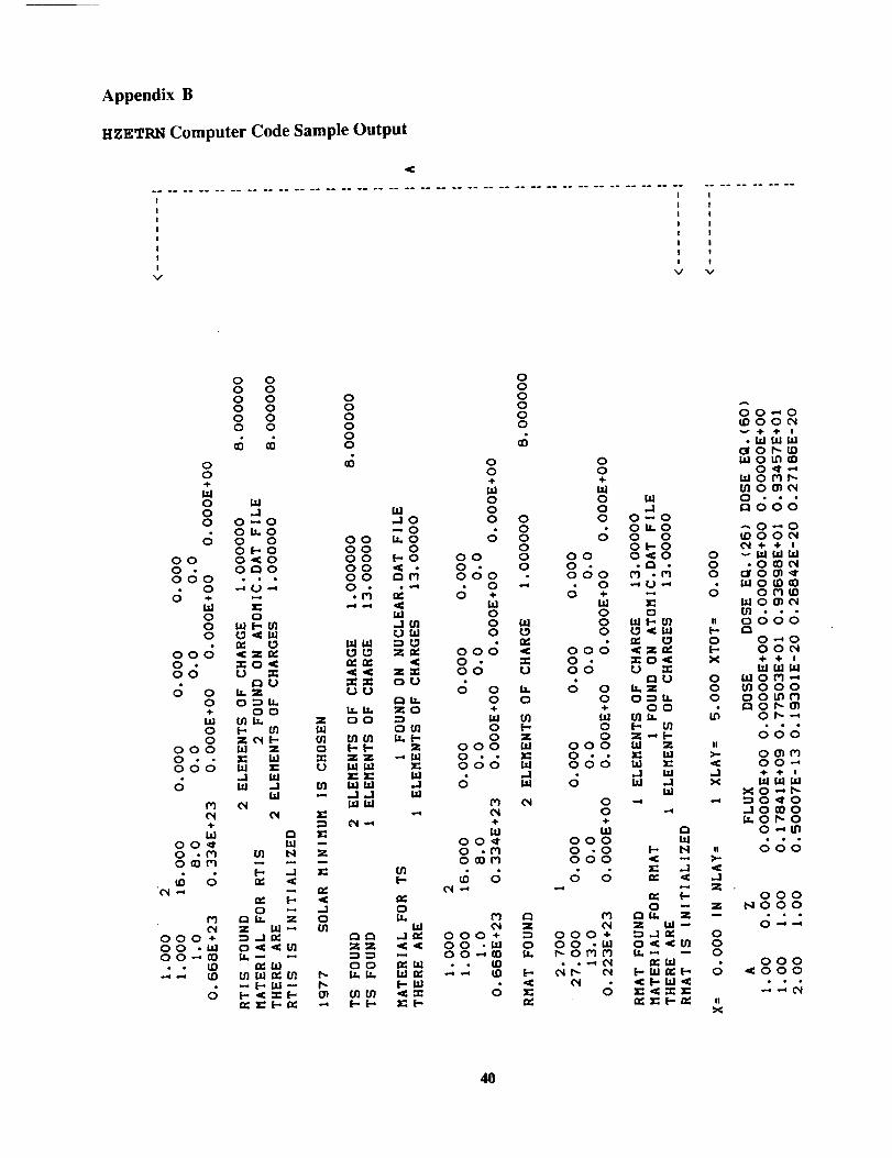
VV V
O00o6
O00066
O00 •O0
6
O00 •O_D
o00O0 •00-,
• •
0o0000
oO+
OOO O
6 oOOOO
O •O --4÷
OO _O _
6 _,c
000000
--0_0
0_040_0
d2
o_m4_
Z_O_
U __U
O _20 0_+ O0
0 _ _0 Z_0 _ Z 0
E _
W --M _
M B N Z
M B_ _ o
÷ _044_
000000
000000
OO÷
000 0
OOO OO OOOO •
6 o -÷
OO _O _
000 4
0-O0
_ o _O o+
O _O _
0000..000
6 _
+
OO_OoMO_M
_ 6
000+00._ o00_
OO÷
000
6OOO-OOO
6 o÷OOO
006O066 o
O+
OO
OOOO •oo_
6OO÷
OOOO.OOOO
6 6
000+00-__OMM
6
.20--001_00 00 [-"00'_0
m .r4
oul C-, m
oo
[-- I/1
-1 II1bl .1
bl
!--. N
O
044 r._
-,'_U
_: [.-. I_14
_) 0.._ 0(D 000_
. I_11xl Ldor 0 I'- _0b l 0 U) (D
0 _1" --,Ixl 0 M I'-in 00_ O_0_666--0._0U) OOC401++
0 _1_11_10 .O_C_0 C;O_
, 0000
0 0.40_-- 0001X 4- + i
lxl Izi l.d0 _.I0 M ,"0 _0000 O010M
Oh--,
666II
_.. O0"_M4 00-'..I + ÷ i
ILl Ixl f._l
-_ :POLO.I0_0_OP'O
O-_LO
,, 666
.J_,
000NO00
000
000<_ ,_000
i!x
411
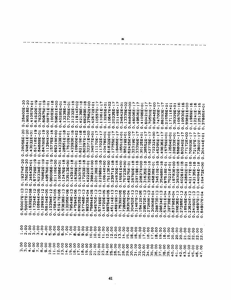
00__0_0_0_0_0
II_|llll÷
O_O0_M_0--__0_O_M_O___0_0_
eleooJeeo
000000000
00_--_0_0_0_0_0_0ll+lll÷l+
__0_
O_O_M_M
000000000
00__0_0_0_0_0
I1+11111+
_M_O_MO_M_O_
_hM_h_--M__M_Q_h_MM_MM_h_M_¢_
000000000000000000000000000000000000000000000
MM_M_M_M_M_MSMM_MM_MM_MM_MM_MM_MM_MMM__0_0_0_00_0--0_00_00_000_0_0_000_0----_0
il+l+l+l÷+l+l+li++ll++ll#+÷ll+ll+ll÷++ll+lll+
__M___IO_O____M__O_O0_O_M__M_____O_MO_M__OOOMM_M__O_M___M_____O0_hOS_O_--MM_h_h_h_D_hS_O--_hO_h_M_h_M¢¢___--_h_h__hMMM_QQMQQ_M©_Q--_QQ_
ooooooooooooooooooooooooooooooooooooooooooooo
000000000000000000000000000000000000000000000000000000000000000000000000000000000000000000
000000000000000000000000000000000000000000000000000000000000000000000000000000000000000000
41

V
_0_0_0--000IOli+i÷i÷|÷
00000000000
_0_0_0_000I+11+1+1÷1÷'
MO__O_
_M_M_0_0_0_
00000000000
_0_0_--__0_0_0_000
III1÷1÷1÷11
_O_MO___M_O_O_O___M ___O_M_ O0
........... _00000000000 O_
O_M_MM_M_M_M_ Oh_0_0--0 _000 O_
l+ll+l+l@+÷ _
_OWO_M_O__0_0__ _MO_M_M_M_ O0_MM_MM_ li
00000000000 O_O_O_O_
00000000000ooooooooooo
00000000000 _00000000000 - -
_0__ ----
(J
0__000000+÷÷÷÷&
v __0_0OM_M_0__
000000
0__000000÷÷÷_÷÷
O_O_OMOMM_OO_M_
000000
000000÷÷÷+÷+
0__0_0O_MM_
000000
0__000000÷÷÷÷+÷
0_--0__0__
000000
H II II i! 11 I!
000000
0 ^0 __
II __
z__
z 0_00_IlIIlI--_
NNNnlI.O vvv
_NNN000111111
_vvv
_OO
I
I
I
V
M0@
1,1O(N
SM
+
6
÷
+
p..
||
CO
t_
0
-1
.1
[...
[-.
V v
000
000000000000000
II II II II II
00000
000000000000000e.e_e
II II fl It II
JJJJJXXXXX
II II II II
_JJJJ_ZZ_Z
Z_ZZZ
000000000000000
II |1 II II II
A
00_00_--_00000000
.____h_M--_MM__0__
__hMh__0_
_00000000
_0_00_--_00000000_@@+@÷+II
._W_MO0_O_O_M_M__
_M_OM__M_
000000000
_00_00000000
l@@+l+ll
,____MM_M_O_O_M0_0_0__0_0_
M_M_MM_
00000000
00000000++++@+@+
D_M__M_J_O0__
66666666
00000000NO0000000
00000000_00000000
42

_0
0000
OOM_MM
M_M_M_
_6GSS6_0_0_000000I+1++1
__M
MO_MM0___M_Mq
6_GSGS
000000II1++1
M_M__0_0
000000
000000
__M_M__M_M_M
_--_O_--__--_OM------_O__O0_O_--_--O_00000000000000000000000000000000000000000
+l+ll++ll++ll+++ll+ll+ll+÷+l++ll++l+l++
_MM_O_M__h_0_©____©©M___MM__DDMM_5_*O_--D_--_O_M_--D_MS_B_MM--_OM_DD_M--O_M_M_MM__M_MDO_--_OS_--SOM_OMOM__DS_M_DD_M_
_666ooooooooooooooooooooooooooooooooooo
_--_O_O__--OM_O_O_O0_O_O_000000000000000000000000000000000000000÷ o ÷ o a ÷÷ t a ÷+ o o ÷÷÷ o , ÷ n t ÷ a a ÷÷ ÷ o ÷÷ n o ÷ ÷ u ÷ o ÷÷
O_MDM_M_DM_D--_M_M_BM--MDM_M_D_O___MSMMMM__M_DM_S_M_D_M_--_S_----M_O--MM_85_O__--_--_MOM--_M_--__ODO_O_MS_MSOO_--O_--_5__--O------OM
SSSSSSSSSSSSGSGGSGGGGSSSSSSSSGGSSGSSSGS
O__O_O_O0_OM_M_O_MM_O_O_000000000000000000000000000000000000000+1+111+111+11++111÷1111111÷111111+1111+
MM_O_M__OM_M__M___O_--M____O0__M____O__O_O_M_MOM_O_O_OO_M_M_O0_O0_MM*OOOO_M_MMMDDS_M_O_OD--OS_M--MM_Q__M__--_M--_h©¢_h_--_M_h_M_
SoooooSooooooooooooooooooooooooo6666666
000000000000000000000000000000000000000÷++_÷÷÷_÷÷÷÷÷÷÷÷÷+++÷÷÷+_÷÷+÷_÷÷÷÷÷÷÷÷÷
______O_+_O_O__M_
__M___O_MO___M_O_
666600000600000000000000000000000000000000000
000000000000000000000000000000000000000000000000000000000000000000000000000000000000000000
000000000000000000000000000000000000000000000000000000000000000000000000000000000000000000
43

bU
0__000000÷÷÷_÷÷
v v __
oeelel
000000
0__000000÷÷÷_÷÷
__0
..e,ee
0_0_0 000000000000
_ _ 000000__00 n + ÷ + + +
_00_ O_O_M__ M_MM_
0_0_0 _ _000000 000000÷÷÷+1+ ÷÷÷÷÷÷
_ _ __0__h_hO _M___M_ ____M ......_ _ 000000
000000 oo . . . . no
_0_ _ 000000000000 0 __
__0 _ __
__ O0 0 ......__M_ ++ 0 ............ _ 0 __
000000 O_ __o- _
M_M_M_ Oh h__000000 0 _ _0_--_÷ ÷ _ + + + _ __
_hM_M O0 X ......_MO_ _ _
_ _0_ O0 _ __
......O_ _ __O_ -- _--_O_ _ __O_ -- __
000000 ---- _ 0 _00_oo0o0o oo _ ,,,,. _...... _ _.00.
__ .. _ vvv__ XX _NNN
_ _ O00U#IO
_ _ _vvv000000 _ _ M_000000 -- > _
I
I
I
V
M0.,1.
0
6
0+
6
0÷
0÷
Wl
II
0
Lrl
,-I
t/1
o
V V
000000000000000
ee,,e
00000
000o0
000000000000000
eee*_
II II II _ I!
_XXXX
n _ _ ii ii
000000000000000
_0
81 II II II II
Xxxxx
0_00__--_0--__00000000000000000_÷÷÷÷÷÷11111÷÷1÷1÷
.______O__M___O_M_OO_M__
_O___M_W___0__
O,eo.ee.eeee,eeeee
_00000000000000000
_00__--_0_0__00000000000000000_÷÷÷÷÷÷IIIII÷÷I÷÷÷
.______O--_M_O0_O____0___0_
__M_MM__O¢
_e.,_eee.e,e.e,e..
000000000000000000
_00__00_0_000000000000000000
I+++I+IIIII++I÷I÷
O_M_B¢O_O_Mh¢____O_M_
66666666666666666
00000000000000000@ @ ÷ ÷ ÷ + + + + + ÷ @ ÷ ÷ @ + @
_0 __M_M __ _
__ _M_O__O_ _i__MO_M_h_O
h_M__M_M_hMe_e.eeeeeeee,e*
6 ooooooooooooooo
00000000000000000_00000000000000000
• e e._eeeeeee_ee
00000000000000000_00000000000000000
44

V
_O_O--O_O0_OM_O_--O_O0_--O_O_O_O_O_O000000000000000000000000000000000000000000II÷÷÷I@÷÷@÷÷÷II÷II÷II÷÷÷I÷÷II÷÷@÷I÷÷÷÷@÷I÷
M_M___O__O_M_M_M_--O_M_O_M_OM_O__M_M__M_MO_O__O_O_O_M_MO___O_O_O00__O_
000000000000000000000000000000000000000000
_O_O__OM--_O_--O0_O0_O_O_O_O_O_O000000000000000000000000000000000000000000
_W__O_M_O_M_________M_--_O_O_M___O__ __0__0_ MM__O_M__O_OM__ ____O0_OM__O_O_M_M__O_
000000000000000000000000000000000000000000
_O_O_O_O_M___M__--__O_000000000000000000000000000000000000000000
lll+lll+lll÷lll÷lllllllllllllllllllllll÷li
__O_O0__M__O_M____MO_O__Oh_MO_hh_hO_O_M_hhO_MO_M_h__ __M_MOh_O_h_hOOM¢_O_M__O_¢h_MM$OM_ O0_M_¢_h_M__MM_¢h__©N¢_MN©_h_M_ + +
000000000000000000000000000000000000000000 O_O_
_¢_¢_--M¢_M__M_M_MCMM_MCM_M O_000000000000000000000000000000000000000000 O_+ ++÷+ +÷++÷÷+ +++++÷++++++ +++ +++++++÷+ ++ ÷+++ _
MM_OBOh_h_M_MO_¢_O_MM_BOhOOM__h_ O0____M_M___O__M___Mh_MO_O_h_hh_M_OBh_OMOhM_O$O_O ___MMh_O_M_h_MMM¢_hOM_hhM_MhOM_h_ O0M___M__h_M_M_h__MM_MM_© , _
000000000000000000000000000000000000000000 O_O_O_O_
000000000000000000000000000000000000000000000000000000000000000000000000000000000000 O0
000000000000000000000000000000000000000000 _000000000000000000000000000000000000000000
45

000000+÷÷+++
_o_mm
0welwJ
000000
0000o0
_O_OM_
oeeeee
000000
000000
000000
000000÷_÷÷÷+
000000
II U il II II II
000000
0 __
0_0o_
NNNliiltivvv
_NNN000111111
_vvv
_00
I
I
I
V
0+
_tLO
(_
÷
÷
0
||
e'l
io
e-i
ul
I/1..3
V V
000000000000000000000000000000
0000000000
IIIIIIIIIIIII1_11$1
0000000000
000000000000000000000000000000
0000000000
II II _ II I! I! II I! II I!
XX_XXX_XX
000000000000000000000000000000
II il If II II II li n ii II
_x_x
0_00__0_00_--0__000000000000000000000v+÷÷_++lllll_÷l+_+ll÷÷
._________0__0___0_0____
___ _0_0_0_0_0_0____
_000000000000000000000
_ _00__0_00_0 __000000000000000000000_+÷÷+÷illlll++l+÷+ll÷t
._0__0_0_____0__00__0_____0_00_
0_____0_
0000000000000000000000
0_00__00_0_0_0000000000000000000000÷ + + ÷ I i I I I I I + + I + I ÷ I I I i
l___O__O0___0__0__0_______
000000000000000000000÷÷÷÷÷÷÷÷_÷÷÷÷÷÷÷_÷_÷÷
_0__0_0_0_0_______0____0___0_00____0_0__0_0_0
__h__h_MCM
000000000000000000000
000000000000000000000NO00000000000000000000
000000000000000000000_000000000000000000000
46

V
÷
v0
6
0÷
0
O_O_O00_OM__O_O00_O0_O_O0_O0000_O00000000000000000000000000000000000000÷i_÷@÷÷÷÷ll÷ll÷lI÷+÷l÷+ll÷÷÷÷l÷÷÷@÷÷l÷ 0
__W_______W_ 0_0____0____00__ +O______M_O_O___M__hMhMO_h_OMOhM_MM_O___hh_¢__M___O__O0_O__ 0
oooooooooooooooooooooooooooooooooooooo
0_0_0_0_0_0_000_00_00_0_00000_000000000000000000000000000000000000000 0+I÷+II@+@II÷II@II÷@÷I÷@I_÷+I+|@÷÷÷@÷I÷ +
h¢_O¢O__O_hhhBM_M_MBMO_M__O_O_h_h__h__M_hM_M_M_O¢¢_hbh_MM_b__M_¢_O¢_MOh_Mbbb
00000000000000000000000000000000000000
_O_O__M--___M___--O_ _
00000000000000000000000000000000000000 0lll@lll+lllllllllllllllllllllllllll+ll _
OhM_MO%_O_h_O_h__B_O_O_h_ 0_h__hh_M_M_Oh_Oh__O0_©_ _h_M__M_O_©_--_O_M__©_ __"*M_--_h_h_--O_--O_--_--_O_S_--_MM O0 0___--_--_M_M_M__©_Mh_M_ + + 0
00000000000000000000000000000000000000 O_
_¢_¢_¢_M_M__M_M_MCMMCM_M_M Oh _00000000000000000000000000000000000000 O_÷÷÷ +÷ ÷ + ÷ + ÷ ÷ ÷ ÷ ÷ +÷÷÷ ÷÷÷ ÷ + ÷ ÷ ÷ ÷ ÷ ÷ ÷÷ ÷ + +÷ + + ÷ _
hhhO_OO_O_M_©M_©_©M_©__M_--_ O0_ _W h _ _ 0 _ _ M _ 0 _ _ _._h _©_ _ _ _ _ _ _ _ _ _ h _ _ _ _ _• M_OW_O_Oh_MhO_hOO_OO_O_OOOB_h_M _ h_hO_M_MB__MO_O_OMM_MMh_M_O_MO O0 ¢
00000000000000000000000000000000000000 O_ _O_ --O_ _O_ --
00000000000000000000000000000000000000 ---- _ 000000000000000000000000000000000000000 O0 _ .
N
00000000000000000000000000000000000000 _00000000000000000000000000000000000000 - -
ee_ee_e_e_ee_leeeeeeee_eeeeeeee_ _
_MM_h©_O_M¢_h_O_M_h_O_MM_h_ ----_M__MMMMMMMMMM_ ¢_ ¢ _ _ _ _ ¢___ _E
47

I
00000÷÷÷÷÷
o_m_o
66S6S
00000÷÷_÷÷
.,0ee
00000
_0000000
.le.e
00000
00000÷++÷÷
_0_0__
00000
il II II |i X
gogoovvvvv
_00_
N N. .VVV
0 0 J! I! I!
_vvv
I
!
V
0÷
ID
_0
ol0÷
o0O0
0¢t0O0-4.
00
c;
O0÷0
mOmOf"lO
6.-:|l
ot, J
-o
Ul
..-1
-.I
m
0 0 00 0 00 0 00 0 00 0 00 0 0
V
00÷
00
_0 0 0--0--0 -- 0_0_0 0 0 0
0 0_0_0 O0 0_0_0 O- 0_0_. 000 • •
&- 6 o+ -d-
o 0
_ 000 _Z_
O, _0__ O0 _OU
0 0 _
_o ÷ O0
o_ 0 _
000 _
000 _
00_0-_ _ N
0 o
_ 000÷ __ 00-_ 0_
V
A
0 --, O_ -, 00 --_ --_ --, O_ -, -', 0 --, --, 00 -', -, -'_ 0_000000000000000000000v 4- 4- ÷ + ÷ I- I I I I I + I- I + 4. 4- I I ÷
b.lO_OiO-.,OiOOP1iO_O_l--,iOLq _t-,O]P1¢O_
ClO0000000000000000000
_000000000000000000000_ + + 4" 4" 4" + I ! I I I + .I- I + + + I I +
0 "_ _'_Ld_.l_al_.i_.ll._"_Ur'_'_Ld_l:J_0 .P'IP'I--,O-,IFI,-,Oi_r O_I'OI_,_ID_)_-,IOPI0 _ _0 O_ _0 _- 0 _ -_ _ -_ _5 -- _ 00 _ _- _ -- bO 0
6 '"om _'_ m _°'__°°_°_" m" " n ° _'_ © ° °
mm 000000000000000000000
0 00l 00 --_-, _ -, Ol --,-, 00 --,0 -, 0 ,.-,-_ --,00000000000000000000
X ÷ ÷ ÷ + I + I I I I I + ÷ I ÷ I + I I I
I,t.I I.d l_.l I_l I_ L1.11_11.d I._l I_11_i l,t.I I.LI I,_l IJ,I I_l I._l i_l I_l I_0 I.__ I_Itq O_ O_ -_ M ," I00l 0 ;_ I0 h- I_"_ 00 ID h"0 ;;ItO iO I_ ¢I"f5 tO 0 I_II_ _ _0 U_ ¢0 ct 0 U) -' _) ID -'_0 0 _" _0 LO tO _ _0 _ --, _ O_ I_ f'- _ _ ID -.._ ,¢ O_ _ h-• _'_OVI--PI_I&'I_D-elPI--,tO.-,_ elP'l-_--.
00000000000000000000J!
,_ 00000000000000000000.._ ÷ ÷ + ÷ + + ÷ + + + + + + + ÷ + + + + +X IJ.I I_l l.r.I I_ I.d _ I.t.I I_ I_i I_ I:,l I_ L_ I.t.I l.rJ ILl I_l i_ I.d I_
Ol =) I_ Ot _l) _ _ ,_" OI P1GD Ol 01 _ Ot I_! _ 0 _ III _ -.,
00000000000000000000
Z
000
II
00000000000000000000NO0000000000000000000
00000000000000000000_00000000000000000000
48

v V
_0_0_000--0_--_000000000000000
_OM____O_MO_h_OMO_
___MM_M_M
000000000000000
--0--0_----0 _0_0--_000000000000000÷÷1_÷11÷÷÷11÷11
__O_M__M_ _0_ O_ _0_MO_____O__MM_
oooooooooooo O_O_O__MO00000000000000+ I I I ÷ I | I ÷ I ! I I I I
_O_M_MO_O_
M_M__M_O
oooooooooooo444
000000000000000
--_O_O0_©O_M___0_0__M_ O_ _O_O_M_O%_O_M_M__
ooooooooooooSSS
0_--000_00_0_00_00000_--0O00000000000000000000000
©_0___00_____O_O__M__MM_O______0_--_00__0____M_hQ__Q©__
000000000000000000000000
0_000_00_--00_0_00000_0O00000000000000000000000+11+++1++11÷+1+1+÷+÷+÷1÷
__M_M_O_M__O__B__M__MMM_MS___M__O_M_MO_M_M__M_M_B___
000000000000000000000000
___M___O_000000000000000000000000
IIIIIIIIIIIIIIIIIIII1+11
_0___0_0_ _M_O_O__--O0_____O_M____ __O_--O_¢_O__MM O0
000000000000000000000000 O_O_
_MM__M_MM_M_MM_M_M_M O_O00000000000000000000000 O_÷÷+÷÷÷÷+÷÷÷÷÷÷÷÷÷÷÷÷_+÷÷ _
O©_O0_O0_O_O00©__©M __©MO_O_OMM__Mh©M_OMMO O0_h_Q__M__M__ I I
000000000000000000000000 O_
O_O_O_
O00000000000000000000000000000000000000ooooooooooooooooooooooooooooooooooooooo oo
O00_MMMM__h_h©_©_OOO_MMMMMM¢¢¢_h© . .
O00000000000000000000000000000000000000 _O00000000000000000000000000000000000000 - -
O_M¢_h©_O_MM_h_O_M_N_O_M_h_ ----_MMdMMMMM_MMMMMMMMMM_____ ==
o..3,.10b.
000
6
fl
N
N
k
Z
W_J
n,.
49

o
I
I
!
V
000000 0÷÷÷÷÷÷ ÷
0___0_0
oDiee*
000000
000000 0÷+÷÷÷÷ ÷
_0_
ee_QIe
000000
0_00000000 0÷÷÷÷÷_ ÷
__ 00__ 0
000000
000000 0_÷÷÷÷÷ ÷
_0__0_
000000
II U I¢ i! II i| i!
J0_00_
vvv_NNNO00ttul!_vvv 0
_00
V V
000
II
_.-o
o
000
,, o
--I -"*
C)_.U.'r.
E-"J" Ol l.l.I.I.I 0
U. O.U,. u I.LII.ILI_" l-
t3 ,...I
C)--OO,. 0U] l" 0"_ n_ ,
_Lq
_I rJ [,-.
r.j ,-n Ol
0__000_._0_--00--_0--0--0_000 __00000000000000000000000000000v_+++÷+lllll++l++÷ll_+÷l++_÷+÷
.__ _______ _
_0_____0___
__ _0_ _0--__ _0-- 0
_00000000000000000000000000000
_000_._--0_00--_--0_0_0_0--_00000000000000000000000000000_÷+÷+++IIIII÷÷I÷+÷II÷++I++II÷÷
0 ______ ___ _0 .__ __0__0__0_0 ___ _0__@_0__-
__0_00___0_________00_0_
. 000000000000000000000000000000
0 _0_ _ __00_0_ 0 _ _0 _0_0.00000000000000000000000000000
I++ll+lllll+÷l+l+lll+lll+lll+
0 __0__ __0___0_0 ___0 __0_0__0_0 0__ _ _0__0_0__ _0__ _
__ _0___ _ _0__0_ _
ooooooooooo60000ooo ooooo6666I!
00000000000000000000000000000++÷÷÷++++÷++++÷÷++++++÷÷+++++
__ _0___ ___0__0_ ___0_ _ _ _0_00___ ___0_ _ _ __0_0_0_ _0_0_0_0_ _0__
00000000000000000000000000000I!
-1Z
000
U
00000000000000000000000000000
NO0000000000000000000000000000ieeeeeeeeeeoee _eeeeooeee_ee_
0______000__
00000000000000000000000000000_00000000000000000000000000000
5O

V
O_----_O_--OOO_OO_OOOO_OOOOO----OOOOOOOOOOOOOOOOOOOOOOOOOOOOOOO+11+11+11+++1+*1|++++|++÷++÷1*
_O_O_MO____O_O____OO__O__
M_M__M_©_M_M__©_©_©_
OOOOOOOOOOOOOOOOOOOOOOOOOOOOOO
OM_O_O_OOO_OO_OO_O_OOOOO_OOOOOOOOOOOOOOOOOOOOOOOOOOOOOOO
MO__OOM_O_MM_M_M_M_M__M_--__M_OO_MM___M_M_O_O__O_OO___M_M__©__©_M_h_M__M
000000000000006660000000000000_______0_OOOOOOOOOOOOOOOOOOOOOOOOOOOOOOIIIIIIlllllllllllllllllllll+ll
___O_O_ _O_____O___O___M_O©_Oh_OhM_O_M___¢_h _W_O%MOM_M_--_--__M_SD_OS-- OO_--_MMM_--_M--BM_M_M_M_---- + +
leillllllllJlJJlllllJtilJlllli _
OOOOOOOOOOOOOOOOOOOOOOOOOOOOOO O_O--
_M_M_M__MM_M_M_MM_M_M_ O_OOOOOOOOOOOOOOOOOOOOOOOOOOOOOO OH+@@÷@++@@÷÷÷+÷@÷+÷++÷÷+@÷+_+@÷ _
mmmmmmmmmmmmmmmmmmmmmmmmmmmmmm
M{_--_O_{_O_O_{M_OO_M_eM__MBBM--___M_OMOM_ _5MS--O_M_%__O_--_DDMS--OD OO__©"____M_¢NCM II
000000000000000000000000000000 O_O_O_O_
000000000000000000000000000000 • •OOOOOOOOOOOOOOOOOOOOOOOOOOOOOO OO
OOOOOOOOOOOOOOOOOOOOOOOOOOOOOO _000000000000000000000000000000 - -
_O___O_M__O__ _--_MMMMMMMMMM____B_ _=
!
OOOOOO++++÷÷
v __
_M_
OOOOOO
OOOOOO÷++÷+÷
OOOOOO
_OOOOOOOOI@+++÷
_0_
OOOOOO
OOOOOO+++÷÷÷
m_oo_
OOOOOO
0 __
0 e.i..o
Ilitii
O_OO_
NNN...vvv
_=_NNN000..._vvv
O__OO
I
!
V
o_O÷
_DI',-tO
6
O÷
ID
ID
6
O÷
_uOO_
6
0+
M
6I!
@
o
o
.1
.J
o[-
51

V
0_000_--_0_00_0--0--0_000_0__0_000__000000000000000000000000000000000000000000++÷÷÷÷÷IIIII++I÷+@II@÷+I+_+÷÷÷÷II+II÷II+÷÷I
0 _00_ _W_M_O______O_M__O0__WO_O_M_M_M_O_M_O_MOW_
__W_ _MO__O____O__W_M___OO__MM_--MOM_O_M_OO__M_M
_OOOOOOOOOOOOOOOOOOOOOOOOOOOOOOOOOOOOOOOOOO
A .-,e4 0 0 0 -_ -, --_-, -..-, 0 --,--,0 0 -, --,--,0 0 0 --,0 --_0 --,0 --,0 M --_0 --,_ 0 _ _ 0 0 0 __OOOOOOOOOOOOOOOOOOOOOOOOOOOOOOOOOOOOOOOOOOO(_i "I" 4- '4- '4- 4" 4" I I I ! I 4" 4- I 4. 4- 4" I I @ 4" 4" I '@ ÷ '4- I +4- ÷ I I 4- I I 4" I I 4. 4" 4- I
O -_ _r_r,_,_,_-_,*b_,_b_,_,*_r_r_hl_,*_r________O • _OO_M--,_OO_O_O_WO_'-O4_O_'-,_ _-_O_O_O__ _O__O_O _ _- _ _OLOM-_OM_DO_D_-_-_MO_O _O_'_OO_O__ _ _ _M O_M
,, o_6_ooooooooooooooooooooooooo6ooooooooo_666
r- OOOOOOOOOOOOOOOOOOOOOOOOOOOOOOOOOOOOOOOOOOI '41" .41. I I + I I I I I ÷ 4" I 4" I 4" i I I + I I I + I I I @ I i I I I ! I I I I I I I
O _ M _ _) O_ O O _ r- _O O_ _- -- -- O O _O O4 _ -_ _" _O _ O_ _O O_ _ O _ _ _ _ _ _ O O _ _ _ _ _ _ _O _ O _ M O_ _ -_ M O_ _O _O M _ M M _ O_ _) " _O O _O _" _ _D _" O M _" _ _ O O _ _ W _ _ _ _ _ _ _O O M -- O -_ (D _- _ (_ ,- _D O _'-_- _ O_ _ _O IO hO _ M O_ M _ _ M _ _ _ _ _ _ _ _ _ _ _ O M _ _ _• _'%,_ M M _'-_ M _-.,(_0_'- 00St_'_M _ _0_ C4M S_O_ OP'- _'_ _--0_ _ MS _ _ M 0 _
666666666ooooo6ooooooooooooooooooooooo6666m!
OOOOOOOOOOOOOOOOOOOOOOOOOOOOOOOOOOOOOOOOOO_I 4"+ + ÷ + 4" '4- 4" as" 4,+4-4. 4" 4" '4- ÷ 4" -I- "k 4' -k "I" 4' "41. '41. 4"4.4" 4" @ ÷ @ -k "1"4" "l" 4" 4" 4" @ 4-
666666666666666666666666666666666666666666)-
..3
ZN
000
d
f!x
OOOOOOOOOOOOOOOOOOOOOOOOOOOOOOOOOOOOOOOOOO_OOOOOOOOOOOOOOOOOOOOOOOOOOOOOOOOOOOOOOOOOO
000000000000000000000000000000000000000000_OOOOOOOOOOOOOOOOOOOOOOOOOOOOOOOOOOOOOOOOOO
----_--_""_"_M_M_MMMMMMMMMM_
52

v
00_0000_00000_--000000000000000000@@11÷÷÷÷1÷@÷÷÷÷1÷
_Mh_OMh_Mh_O_M__ __M_
00000000000000000
00_00_0_00000_000000000000000000+÷ , _ ++ , + i +++÷++ i +
____0___M__O___W_O_M__O___M_MO____M_
66666666666666666_M___O_00000000000000000
IIIIIIII|II||I+II
Mh_OOB_hMh_O_h__M_OMWO_M_M_M_M_O__ ____0_0_0 O0_M_M_M_hM_M_ ÷ +
66666660000000000O_
MMMMM_MCMMCM_M_MM O_00000000000000000 O_÷ ÷ ÷ ÷ + @ + ÷ + ÷ + + @ + @ ÷ + _
_O_M___0_0__0__ __O_%00%_M_hO O0__M__M_MM II
00000000000000000 O_O_O_O_
00000000000000000 • •00000000000000000 O0
00000000000000000 _00000000000000000 - -
_M_ _O_M_© ----
000000++÷@++
v ___0_
000000
000000÷@@+÷÷
000000
_00000000I÷+÷++
M_M__M_O___M
000000
000000+++@++
_M_M_O_
000000
HIIIIHHO
000000
0 ......
0 __
0_00_lilil|_5_
0 vvv
_vvv 0M_
_00
ii!
v
0@
f.,tJOI
0+
M
ID
6
÷
_0
+
M
6
oCl
v
0--_000_--_0000000000_@+@@_+il;l
.___OWM_MO0_
___M_
_0000000000
_000_----_0000000000_+÷@@++;III
0 ___0 ._ _0_0_0_0 _M_ _M
_O_hM_hh_M_MMO_
. 00000000000
0 _0__0000000000l÷@ll+llll
0 __MO_M_h_0 _O__M_O0 0_00_0_0_
_MM_M___M_
0000000000
0000000000
_M_____00_____0_M___
___M
0000000000U
.,.3
Z
II
0000000000_0000000000
0000000000_0000000000
53

_0_00_0_0_0_000_0000000000000000000
I++1+++|1+++1++++++
M__M_M__M
0__0_0_0___M_M_OM¢_O__O___M____
0000000000000000000
_0_00_000_0_0_0_0000000000000000000
___W_O_ _0_0__00_0_ _MO_
_O0_O_OM_O__M_h_M_©___
0000000000000000000
_00_0_0_0_0_00000000000000000000
J++|+t+liJ+JJl+JJJ+
_O_BOhBhMM_h_M_ _ __OOO_ ___M_@___hOM__O__O__M_O_
0_0_0_000_00_00000000000000000000000+fJ+J|+|J+++J++|i+++
M__M_O_M_O__ ____M_ _____M___h_h¢_MOh_M_O__M_M_M_¢_M_
00000000000000000000
0_0_0_000_00_00_00000000000000000000+ll+ll+ll+++l++ll++l
__¢_O0_M_O¢_MChCM_M_O_M_M__O___OOM_O_O0__OO0____O00_M_
0_0000000000+l++++
_M__M_O_M_
0_0000000000
_0_0
_0_
000000000000000000000000000000000000000000000
__¢¢_ _B_B_M_M_M__MMM_MCMMMMCM_000000000000000000000000000000000000000000000+++++++++++++++++++++++++++++++++++++++++++++
__O_M___O_OO____M_M__#_O_MM_M__O___M_O_O____M_M_O_O_O__M__O__M_O_O0__M_M_B¢_¢_h_h_M_h_M_¢_h_h_M_OO_¢O__O__¢Mh___h__M__h_¢_M_M_
000000000000000000000000000000000000000000000
000000000000000000000000000000000000000000000000000000000000000000000000000000000000000000
000000000000000000000000000000000000000000000000000000000000000000000000000000000000000000
54

v
O_O
OOOO
OM_
OOOO
O_OOOOO+ + I ÷
_O_OOM_
OOOO
_O_OOOOI + I I
OO_
_O __O_ OO
OOOO O_O_
M_M O_OOOO O_÷÷+÷ _
M_OO OO
_ OO
OOOO O_O_O_O_
OOOO ..OOOO OO
OOOO _000o --
OOOOOO+ + + + + + V
v I,dl_ bJ£db.l£_l0 _ M('_ _IM_ D,. I_ M 00•.., --, h- I'-- .-, ¢]D
000000
OOOOOO+ + + + + +
00_ _00 _-_
OOOOOO
.",0_ _..',O OOOOOOOI + + + + +
M-_D_MM
66oooo
OOOOOO+ + + + + +
I_l I_1 I_l I.d bJ LilM_OiOiO_
000000
II II II II II II
0000000 iO iO _D iO _0 iO
0 ...... '_0 ---O tOt_ IDtO_
Ill I-, I-, _., I-, i'_ _., in II
-- l.x.. b, b., la, b. II, _i
il 11 II _ _I _ _i_
al vvv ,.l_" _"t.4NN _: 0
B-. O O O . . ol _ OZ b.. b.. I_ v v v 0 0
L_ a:
ILl b. OC3 lan,. b..L_ :_
I
I
I
v
0+
£1.1
d
O
M
4.
6
+
M
||
t_
O--_OOO_--_O----OO_--_OOO__OOOOOOOOOOOOOOOOOOOOOOO_++++++lllll++l+++ll+++l
.______S_M_D_OhO_hSOM--h__--___O_O___O_
_W_O___¢_O___MM__O_BM_O_M_
_OOOOOOOOOOOOOOOOOOOOOOO
_OOO__O----OO_--_OOO--_OOOOOOOOOOOOOOOOOOOOOOO_+ + + + + + I I O I I + + I + + + I I + + + i
O _______0 .__O___M__0 _OOM__O__M_M_
_MO_O_M_M_¢OO__¢h_MM_M_O¢_M__OM
ao 0 O0 O00000000000000000000
0 _0___0_0_0--_0--_OOOOOOOOOOOOOOOOOOOOOOO
l++ll+llllll+l+l+lli+II
0 __O_M_O_O__OO ___0__0__O OOO_MO__W__O_
_MMOMM_O__MM_¢M_OM_
OOOOOOOOOOOOOOOOOOOOOOO
OOOOOOOOOOOOOOOOOOOOOOO+++++++++++++++++++++++
____O_____M_O_O_O_O0_O0____MO_M____M_O__O_MOOM_--_M_
OOOOOOOOOOOOOOOOOOOOOOO
OOOOOOOOOOOOOOOOOOOOOOO_OOOOOOOOOOOOOOOOOOOOOOO
OO OOOOOOOOOOOOOOOOOOOOO_OOOOOOOOOOOOOOOOOOOOOOO
55

...................... ..... .............................................................
V
0--000--0_0_00_000_0000000000000000000+++++++;J+JI++P+++!
_O_OOMOM_MO_M_O0__O__M_O___0_0___0_0___M_M_Mq_
0_0_0_0_0_0_000_0000000000000000000+++1+++11+11+11_++1
O____O_OM___M___M__M_M_O__O__O__M_M_O0_©____MM_M
0000000000000000000
_O_O__M__0000000000000000000
;+l|l+lllllllllllll
_M_O_q__h_©M_
__M_MO0_O___0____0_
00_0000_00000_000000000000000000++11++++|++++++1+
__OM_hBM_BhO_O__M___M___O__M____OO__M___M_
66oooooooooooooo00_00_0_00000_000000000000000000++11++1+1++++++1+
__O_O_M_ _M_M___O__M_O_OM_M__O__ _ ___M___M__ _
00000000000000000
_M___OM_00000000000000000
_O_M_O_M_O_ M_M__O_M_ _0___M_h_OM_Oh__M_ _M__M_
1010OO
_--_©____--M_©M_¢hM__h + +
000000000000000000000000000000000000 O_O_
__M_M_MM_MMM_M_MMMM_MMM_M O_OOOOOOOOOOOOOOOOOOOOOOOOOOOOOOOOOOOO O_+++++++++++÷+++÷++++++++++++++++++++ _
_MO_O_MM_OM__O_O__M_M__ O0_M_N_N _--_O--_MM_h__O__--h _h©_O0__M_h__M_hMO_MM_O_MM __MM___O_OOBhMOMOM__h_M OO__©--_--_M_----_h©___M_¢M_ II
000000000000000000000000000000000000 O_O_O_O_
OOOOOOOOOOOOOOOOOOOOOOOOOOOOOOOOOOOO . .OOOOOOOOOOOOOOOOOOOOOOOOOOOOOOOOOOOO OO
000000000000000000000000000000000000 _000000000000000000000000000000000000 - .
OOOV + + +
666
+ + +
666
! + +
+ + +
n H II
gogC_ U_ _0 lO
..3 6. _-, _..
O 101010
x 660:I- _Cl -J
_:, O...,(%1
_'_ NNN
OOO
b_
56

V
0_000__0_00_--000--0_000_0_--0_0_000000000000000000000000000000000000_+@@+@+lllll@@l+++ll@+@l@@÷+@@@ll@ll@
• __________
_O__O__MO_O_M_O_O_M__O____M_O_O_ _ __MMO_
___M_M___OM_O_O_--M_O
_000000000000000000000000000000000000
_000_--_0--_00_000_0_0_0_0_0--_0_000000000000000000000000000000000000_++++++11111÷+1+++11+++1+++1+++11+11+
0 ___________O .SM_MO_M%M_MO_D_5*DDO_OD_MM0 O____hh_MMM_h_O_©_O_h_M_
_O___O__O___O____MM_O_M_M__O_M_OO__M_
. 0000000000000000000000000000000000000
0 _O___O_O_O__O_O__M_000000000000000000000000000000000000
X I@÷11+111111÷1+1+1111111÷111+1111111
O _hh_¢h__©_hOM¢_©_h_O©O _M_O_M__MO__M_OMM_0 OMO__OB___M__MM_M_M_¢_O
C_MM_%O_O_MM_M_M_MOO_OM_M_5_M_O0___M_M______M_
000000000000000000000000000000000000;!
000000000000000000000000000000000000J ++÷++÷+_÷++÷+÷++@@_@+@@÷@÷@@+÷÷÷@++@
__O_O__O0_O_OM_O___O_M_M_OWMM__Mh__O___M_h_OM__M___OM___O_
___M_h__Mh____M_
ooooooooooooooooooooooooooooooooooooII
.Jz
z
000
II
000000000000000000000000000000000000NO00000000000000000000000000000000000
000000000000000000000000000000000000_000000000000000000000000000000000000
57

v
0_000_00_0000_00000_000000000000000000000000÷ t ÷+÷ t ÷÷ I n ÷÷++ t ÷÷++÷÷ t ÷
__MMMM___OM__M_O_O_OM_M__O_O___MM_M_BOB_M__B__O__M_M__M____
66666666666660000066666_000_00_ _00_0_00000_000000000000000000000000I1÷++1_+11+÷1÷1++÷÷÷÷1+
__MM_O____M__O__O_M__
_M_MM_M_--_©Mh___
66666_66666666_6_6_66___M____OM_00000000000000000000000IIIII!11111111111111÷1!
_O_OM_MMO_MM_OM__M__O__M_O_O_M____ ____M_O_O__ O0___M____ ÷ +
666666ooooooooooooooooo o=
ooooooooooooooooooooooo
_0_____0_M__M_OOO__OMOM___O_O_O__O_O_M_O_OW"_OM___M__M_M_
66666666666666_6_6_6666
0000000000000000000000000000000000000000000000
0 "4
or,-o_
66
O0i I
66
0000000000000000000000000000000000000000000000
_h_O_M_h_O_M_h© ----MMMM_ ¢_____ _
N
I
v
o.l,..10b.
000
ii
!-
[-.z
:2O
[.-
L_...}
I!
V
000000 0÷÷÷÷÷÷ +
_OM 0
000000
000000 0÷÷÷÷÷÷ +
h_M_
666666 6_00000000 0;_÷÷÷÷ ÷
M__
666666 6
000000 0÷÷÷÷+÷ ÷
M_C_ M__ M
000000
0_00_
NNN...vvv
OOOIlllll_vvv O
_00
v
U)_0_0_-00
_66
_MM.U)_D
U_O0
f'% • •
O0
i.!1,,
;,u _ lO
tO_0_0_
0 _JO_D
LU U_ LO
[.. [....,.-,
-I >_ .-I
58

%A V
0000000
_0__0
00
I!
59

mm
000000000000÷+÷+÷÷+÷÷÷÷÷
___0_D_M_M_M__BM_OBMO__0000__0
___ _ _0_O_M_M
_i ...... _O_M_O_--_N _M--_MOD_ _@ _0_ ..... _MO_
_MO__O___MO_O_ ..... _
i
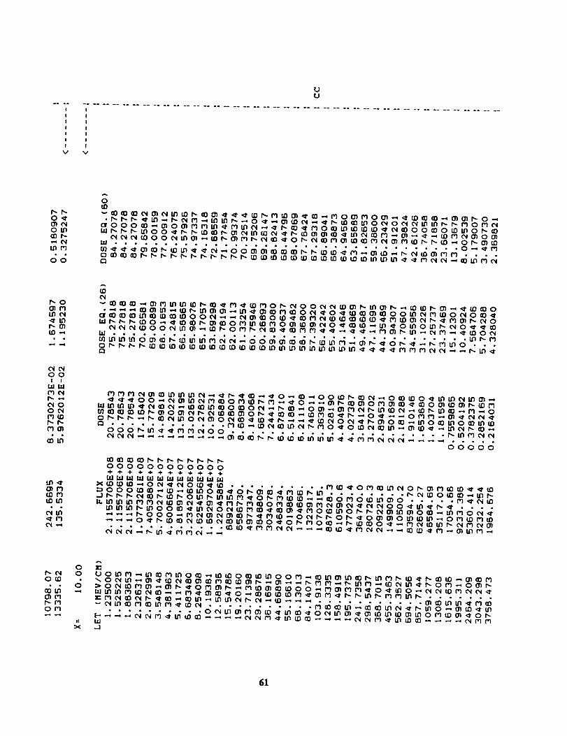
_JU
V V
f,-D-O_
OU_
UIM
6_
_'-0O]MtO0_,,_iOr,-O_tO--,
O0! !
LU_MO_D,, ...,0_0
_0r,-r-MO_
.;u4
61
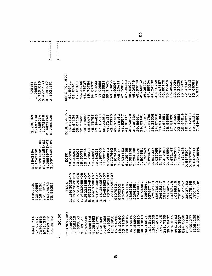
:3Q
V V
_M_
_MO__M--_O_M_0_0_.._M_
0000
_0_
M____0
_M_O.... _
M_..O0
0000111!
_0_
MM___0__M_M_
O0_M
_O_MM_M_
.OMM_
_O_M.
__0_O00MMO_O
_O0_M__OMO0_O
__M_
000000000_+÷÷÷÷÷÷÷
___0
_0 _
_0__M...... _
_M_M
_0_0_
o0 _JOU'_ M,-,_I_ ©M_i'_O_)--_O_O_ _0 _'_OOM.-, _O_h_M h _ _ h ©_
_MO_O_I_- _-_DI_ I_I_OIh-_--_O -_ ........_ e4_ 0 MODISIM _'t901 ........... MODOOI.r)-,OOUIt_I_I'h. LIIO.-_
.......... O0;IDO_O_D _'U'_D_'OO;b')O_O_DI_iOO_I_OM_
62

Ld
v V
0!
_h_M_hO_M_--h_M_O_
_O_O_M__0__0_M_OM_M_
.... _M_M
00000_
_O_M___O__M_OMO_O_m_M
O__M_MO...... _M
0000000;llllll
MO __M_
O_O_M__
_0_0_ _
__0_
_0__
__0
__M_M
0000000000÷+÷÷÷_÷÷÷÷
___0__0_000__MMMM_ __M__
_0__0_
_M_M_M_¢MhChM_O_O_OM_MMM _h_ _

I,b.
V v
0!
_M__M_O_MM__M_O_MMO_ _ _____O_O_M__OM_O__O
_M_OM_"M_
00000_
_O_O_M___M_O__M__OMO_O_M_fl_MM_h_%_
....... _M
0000
0000000
__MO__M_0_____M_O_O_M__
_ _ _0_0_ __%_hMB_M_M_h_M__O_
___0____M_--BM_
_M_m_0___M___M_M
_@_0_0_0_O__M___OM_
_@M_O0 •
_OM_O__O_
.__M_M_M_O__M_M_OM_O_O_OM___M__
64

t_
V V
_00______M
0_0_0__M__M--_
._M_
0000000
_00__M_
--__0__M_BM__M_M_M_M_
O0000000_M_
000000000000÷+÷÷÷÷÷÷÷÷÷÷
__0_0_ ....... _M___OM__h_M •Q___M_M_M__M_
_O__M_O__
O00_MOO__OM__............ _M__

V V
....... _h_M__O_O
O0000000_M_
__M_ _0___
...... ___M_____ .... _0_
M__M_M___
66

V V
........... ___0__MMM__ ...............
O000000%_BMM_
_M_M_M_M_M_O©_Mh_O_h_h_¢_
_MMM_h©_hChM_MMMhO_MB_M_M_O000h¢_QQOMM_QB_
......... _0__M_O0 ......
000000000000÷÷÷÷÷÷÷÷÷÷÷÷
a_mmm_o_ommm__ _O_O_MOM_
__O_M___O0_O_MO_O00_MO0__O............ _
o0 _JOM'_M--,_'$_MM_O _--,t_DO_
-- i'_L_ _ M _D li3M _ i_ (_ ............... 0 (_i_ _
_! i;J
6?

V V
-_M___M_O_
_ M_ 0__O__MMMMM
.............. ______MMMMSS_------_-- ............... •
00000000_ M__
-__OM_SMMM_OhDB*MB___M_
_O_M___$e_eeeeee
_MMM__M_O_MMMMMMMM
........ _0_hhh_MM--O • - •
00000000000÷ ÷ ÷ ÷ ÷ ÷ ÷ ÷ ÷ _ ÷
__0___M_O__M_ _MM___M_MM_
O00MO_B_M__ _0_0O00_ _M__
o ;0 UO[_IM,-,I_ _ML_O_--,
_" 00,I _ M O_ ,--,05 P- _" 0 M
• • $ • • • • • • •
I---,-,--_--,e4 e4r5 _, _')_E).-,
68

i-a
v
69

References
1. Peters, B.: The Nature of Primary Cosmic Radiation. Progress in Cosmic Ray Physics, J. G. Wilson, ed., Interscience Publ.,
Inc., 1958, pp. 191-242,
2. Davis, ]_,everett, Jr.: On the Diffusion of Cosmic Rays in the Galaxy. Proceedings of the Moscow Cosmic Ray Conference,
International Union of Pure and Applied Physics (Moscow), 1960, pp. 220--225.
3. Ginzburg, V. L.; and Syrovatskii, S. I. (H. S. H. Massey, transl., and D. Ter Haar, ed.): The Origin of Cosmic Rays.
Macmillan Publ., 1964.
4. Gloeckler, G.; and Jokipii, J. R.: Physical Basis of the Transport and Composition of Cosmic Rays in the Galaxy. Phys.
Rev. Lett., vol. 22, no. 26, June 30, 1969, pp. 1448-1453.
5. Lezniak, J. A.: The Extension of the Concept of the Cosmic-Ray Path-Length Distribution to Nonrelativistic Energies.
Astrophys. & Space Sci., vol. 63, no. 2, July 1979, pp. 279-293.
6. Wilson, John W.: Analysis of the Theory of High-Energy Ion Transport. NASA TN D-8381, 1977.
7. Wilson, J. W.: Depth-Dose Relations for Heavy Ion Beams. Virginia J. Sci., vol. 28, no. 3, 1977, pp. 136-138.
8. Wilson, John W.: Heavy Ion Transport in the Straight Ahead Approximation. NASA TP-2178, 1983.
9. Wilson, John W.; Townsend, L. W.; Bidasaria, H. B.; Schimmerling, Walter; Wong, Mervyn; and Howard, Jerry: 2°Ne
Depth-Dose Relations in Water. Health Phys., vol. 46, no. 5, May 1984, pp. 1101-1111.
10. Wilson, John W.; Lamkin, Stanley L.; Farhat, Hamidullah; Ganapol, Barry D.; and Townsend, Lawrence W.: A Hierarchy
of Transport Approximations for High Energy Heavy (HZE) Ions. NASA TM-4118, 1989.
11. Wilson, John W.; Townsend, Lawrence W.; and Badavi, E E: A Semiempirical Nuclear Fragmentation Model. Nucl.
lnstrum. & Methods Phys. Res., vol. B18, no. 3, Feb. 1987, pp. 225-231.
12. Wilson, John W.; and Badavi, F. E: Methods of Galactic Heavy Ion Transport. Radiat. Res., vol. 108, 1986, pp. 231-237.
13. Wilson, John W.; and Townsend, L. W.: A Benchmark for Galactic Cosmic-Ray Transport Codes. Radiat. Res., vol. 114,
no. 2, May 1988, pp. 201-206.
14. Curtis, S. B.; Doherty, W. R.; and Wilkinson, M. C.: Study of Radiation Hazards to Man on Extended Near Earth Missions.
NASA CR-1469, 1969.
15. Allkofer, O. C.; and Heinrich, W.: Attenuation of Cosmic Ray Heavy Nuclei Fluxes in the Upper Atmosphere by
Fragmentation. Nucl. Phys., vol. BT1, no. 3, Mar. 25, 1974, pp. 429-438.
16. Chatterjee, A.; Tobias, C. A.; and Lyman, J. T.: Nuclear Fragmentation in Therapeutic and Diagnostic Studies With Heavy
Ions. Spallation Nuclear Reactions and Their Applications, B. S. P. Shen and M. Merker, eds., D. Reidel Publ. Co., 1976,
pp. 169-191.
17. Letaw, John; Tsao, C. H.; and Silberberg, R.: Matrix Methods of Cosmic Ray Propagation. Composition and Origin of
Cosmic Rays, Maurice M. Shapiro, ed., Kluwer Academic Publ., 1983, pp. 337-342.
18. Ganapol, Barry D.; Townsend, Lawrence W.; and Wilson, John W.: Benchmark Solutions for the Galactic Ion Transport
Equations: Energy and Spatially Dependent Problems. NASA TP-2878, 1989.
19. Townsend, Lawrence W.;Ganapol, Barry D.; and Wilson, John W.: Benchmark Solutions for Heavy Ion Transport Code
Validation. Abstracts of Papers for the Thirty-Seventh Annual Meeting of the Radiation Research Society and Ninth Annual
Meeting of the North American Hyperthermia Group, Mar. 1989.
20. Schimmerling, Walter; Miller, Jack; Wong, Mervyn; Rapkin, Marwin; Howard, Jerry; Spieler, Helmut G.; and Janet,
Blair V.: The Fragmentation of 670 A MeV Neon-20 as a Function of Depth in Water. Radiat. Res., vol. 120, 1989,
pp. 36-71.
21. Schimmerling, Walter: Ground-Based Measurements of Galactic Cosmic Ray Fragmentation in Shielding. Adv. Space
Res., vol. 12, no. 2-3, 1992, pp. (2)445-(2)459.
22. Wilson, John W.; Townsend, L. W.; Lamkin, S. L.; and Ganapol, B. D.: A Closed-Form Solution to HZE Propagation.
Radiat. Res., vol. 122, 1990, pp. 223-228.
23. Cleghorn, T. F.; Freier, P. S.; and Waddington, C. J.: The Energy Dependence of the Fragmentation Parameters and Mean
Free Paths of Cosmic-Ray Nuclei With Z > 10. Canadian J. Phys., vol. 46, no. 10, May 1968, pp. $572-$577.
7O

24. Heckman, H. H.; Greiner, D. E.; Lindstrom, P. J.; and Bieser, F. S.: Fragmentation of 14N Nuclei at 29 GeV: Inclusive
Isotope Spectra at0 °. Phys. Rev. Lett., vol. 28, no. 14, Apr. 3, 1972, pp. 926-929.
25. Heckman, H. H.: Heavy Ion Fragmentation Experiments at the Bevatron. NASA CR-142589, 1975.
26. Raisbeck, G. M.; and Yiou, F.: Production Cross Sections of Be Isotopes in C and O Targets Bombarded by 2.8-GeV ix
Particles: Implications for Factorization. Phys. Rev. Lett., vol. 35, no. 3, July 21, 1975, pp. 155-159.
27. Feshbach, H.; and Huang, K.: Fragmentation of Relativistic Heavy lons. Phys. Lett., vol. 47B, no. 4, Nov. 26, 1973,
pp. 300-302.
28. Goldhaber, A. S.: Statistical Models of Fragmentation Processes. Phys. Lett., vol. 53B, no. 4, Dec. 23, 1974, pp. 306-308.
29. Alsmiller, R. G., Jr.; Irving, D. C.; Kinney, W. E.; and Moran, H. S.: The Validity of the Straight-Ahead Approximation in
Space Vehicle Shielding Studies. Second Symposium on Protection Against Radiations in Space, Arthur Reetz, Jr., ed.,
NASA SP-71, 1965, pp. 177-181.
30. Alsmiller, R. G., Jr.; Irving, D. C.; and Moran, H. S.: Validity of the Straightahead Approximation in Space-Vehicle
Shielding Studies, Part II. Nucl. Sci. & Eng., vol. 32, no. 1, Apr. 1968, pp. 56-61.
31. Curtis, S. B.; and Wilkinson, M. C.: The Heavy Particle Hazard--What Physical Data Are Needed? Proceedings of the
National Symposium on Natural and Manmade Radiation in Space, E. A. Warman, ed., NASA TM X-2440, 1972,
pp. 1007-1015.
32. Wilson, John W.; and Lamkin, Stanley L.: Perturbation Theory for Charged-Particle Transport in One Dimension. Nucl.
Sci. & Eng., vol. 57, no. 4, Aug. 1975, pp. 292-299.
33. Wilson, John W.; Townsend, Lawrence W.; Nealy, John E.; Chun, Sang Y.; Hong, B. S.; Buck, Warren W.; Lamkin, S. L.;
Ganapol, Barry D.; Khan, Ferdous; and Cucinotta, Francis A.: BRYNTRN: A Baryon Transport Model. NASA TP-2887,
1989.
34. Wilson, John W.; Townsend, Lawrence W.; Ganapol, Barry; Chun, Sang Y.; and Buck, Warren W.: Charged-Particle
Transport in One Dimension. Nucl. Sci. & Eng., vol. 99, no. 3, July 1988, pp. 285-287.
35. Shinn, Judy L.; John, Sarah; Tripathi, Ram K.; Wilson, John W.; Townsend, Lawrence W.; and Norbury, John W.: Fully
Energy-Dependent HZETRN (A Galactic Cosmic-Ray Transport Code). NASA TP-3243, 1992.
36. Wilson, John W.; Townsend, Lawrence W.; and Badavi, Forooz E: Galactic HZE Propagation Through the Earth's
Atmosphere. Radiat. Res., vol. 109, no. 2, Feb. 1987, pp. 173-183.
37. Shinn, Judy L.; Wilson, John W.; Weyland, Mark; and Cucinotta, Francis A.: Improvements in ComputationalAccuracy of
BRYNTRN (A Baryon Transport Code). NASA TP-3093, 1991.
38. Cucinotta, E A.: Extension of BRYNTRN to Monoenergetic Light ion Beams. NASA TP-3472, 1994.
39. Shinn, Judy L.; and Wilson, John W.: An Efficient HZETRN (A Galactic Cosmic Ray Transport Code). NASA TP-3147,
1992.
40. Yakowitz, Sidney; and Szidarovszky, Ferenc: An Introduction to Numerical Computations, Second ed., Macmillan Publ.,1989.
41. Adams, J. H., Jr.; Silberberg, R.; and Tsao, C. H.: Cosmic Ray Effects on Microelectronics. Part l--The Near-Earth
Particle Environment. NRL Memo. Rep, 4506---Pt. I, U.S. Navy, Aug. 1981. (Available from DTIC as AD AI03 897.)
42. Badhwar, G. D.; and O'Neill, P. M.: Improved Model of Galactic Cosmic Radiation for Space Exploration Missions. Nucl.
Tracks & Radiat. Meas., vol. 20, no. 3, July 1992, pp. 403-410.
43. Adams, James H., Jr.: Cosmic Ray Effects on Microelectronics, Part IV. NRL Memo. Rep. 5901 (Revised), U.S. Navy,
Dec. 31, 1987.
44. Walske, M. C.; and Bethe, H. A.: Asymptotic Formula for Stopping Power of K-Electrons. Phys. Rev., vol. 83, 1951,
pp. 457-458.
45. Bragg, W. H.; and Kleeman, R.: On the ot Particles of Radium, and Their Loss of Range in Passing Through Various Atoms
and Molecules. Philos. Mag. & J. Sci., ser. 6, vol. 10, no. 57, Sept. 1905, pp. 318-340.
46. Sternheimer, R. M.: The Density Effect for the Ionization Loss in Various Materials. Phys. Rev., vol. 88, no. 4,
Nov. 15, 1952, pp. 851-859.
71
47. Armstrong, T. W.; and Alsmiller, R. G., Jr.: An Approximate Density-Effect Correction for the Ionization Loss of Charged
Particles. Nucl. lnstrum. & Methods, vol. 82, 1970, pp. 289-290.
48. Shinn, Judy L.; Farhat, Hamidullah; Badavi, Francis F.; and Wilson, John W.: Polarization Correction for Ionization Loss
in a Galactic Cosmic Ray Transport Code (HZETRN). NASA TM-4443, 1993.
49. Andersen, Hans Henrik; and Ziegler, James F.: Hydrogen Stopping Powers and Ranges in all Elements. Pergamon Press,
Inc., 1977.
50. Janni, Joseph E: Calculations of Energy Loss, Range, Pathlength, Straggling, Multiple Scattering, and the Probability of
Inelastic Nuclear Collisions for 0.1- to 1000-MeV Protons. AFWL-TR-65-150, U.S. Air Force, Sept. 1966. (Available
from DTIC as AD 643 837.)
51. Ziegler, J. F.: Helium-Stopping Powers and Ranges in All Elemental Matter. Pergamon Press, Inc., 1977.
52. Barkas, Walter H.: Nuclear Research Emulsions. Volume 1--Techniques and Theory. Academic Press, 1973.
53. Lindhard, J.; Scharff, M.; and Schiott, H. E.: Range Concepts and Heavy Ion Ranges (Notes on Atomic Collisions, II).
Mat.-Fys. Medd.--K. Dan. Vidensk. Selsk., vol. 33, no. 14, 1963, pp. 142.
54. Wilson, J. W.; and Kamaratos, E.: Mean Excitation Energy for Molecules of Hydrogen and Carbon. Phys. Lett., vol. 85A,
no. I, Sept. 7, 1981, pp. 27-29.
55. Wilson, J. W.; Chang, C. K.; Xu, Y. J.; and Kamaratos, E.: Ionic Bond Effects on the Mean Excitation Energy for Stopping
Power. J. Appl. Phys., vol. 53, no. 2, Feb. 1982, pp. 828-830.
56. Wilson, J. W.; and Xu, Y. J.: Metallic Bond Effects on Mean Excitation Energies for Stopping Powers. Phys. Lett.,
vol. 90A, no. 5, July 12, 1982, pp. 253-255.
57. Wilson, J. W.; and Townsend, L. W.: An Optical Model for Composite Nuclear Scattering. Canadian J. Phys., vol. 59,
no. 11, Nov. 1981, pp. 1569-1576.
58. Bowman, J. D.; Swiatecki, W. J.; and Tsang, C. E: Abrasion and Ablation of Heavy Ions. LBL-2908, Univ. of California,
July 1973.
59. Townsend, L. W.; Wilson, J. W.; Cucinotta, E A.; and Norbury, J. W.: Comparison of Abrasion Model Differences in
Heavy Ion Fragmentation--Optical Versus Geometric Models. Phys. Rev. C, vol. 34, no. 4, Oct. 1986, pp. 1491-1494.
60. Cucinotta, Francis A.; and Dubey, Rajendra R.: Final State Interactions and Inclusive Nuclear Collisions. NASA TP-3353,
1993.
61. Gosset, J.; Gutbrod, H. H.; Meyer, W. G.; Poskanzer, A. M.; Sandoval, A.; Stock, R.; and Westfall, G. D.: Central
Collisions of Relativistic Heavy Ions. Phys. Rev. C, vol. 16, no. 2, Aug. 1977, pp. 629-657.
62. Htifner, J.; Schafer, K.; and Schiarmann, B.: Abrasion-Ablation in Reactions Between Relativistic Heavy Ions. Phys.
Rev. C, vol. 12, no. 6, Dec. 1975, pp. 1888-1898.
63. Morrissey, D. J.; Marsh, W. R.; Otto, R. J.; Loveland, W.; and Seaborg, G. T.: Target Residue Mass and Charge
Distributions in Relativistic Heavy Ion Reactions. Phys. Rev. C, vol. 18, no. 3, Sept. 1978, pp. 1267-1274.
64. Guthrie, Miriam P.: EVAP-4: Another Modification of a Code To Calculate Particle Evaporation From Excited Compound
Nuclei. ORNL-TM-3119, U.S. Atomic Energy Commission, Sept. 10, 1970.
65. Silberberg, R.; Tsao, C. H.; and Shapiro, M. M.: Semiempirical Cross Sections, and Applications to Nuclear Interactions of
Cosmic Rays. Spallation Nuclear Reactions and Their Applications, B. S. P. Shen and M. Merker, eds., D. Reidel Publ.
Co., 1976, pp. 49-81.
66. Silberberg, R.; Tsao, C. H.; and Letaw, John R.: Improvement of Calculations of Cross Sections and Cosmic-Ray
Propagation. Composition and Origin of Cosmic Rays, Maurice M. Shapiro, ed., D. Reidel Publ. Co., 1983, pp. 321-336.
67. Wilson, J. W.; Shinn, J. L.; Townsend, L. W.; Tripathi, R. K.; Badavi, E E; and Chun, W. Y.: NUCFRG2: A Semiempirical
Nuclear Fragmentation Mode/. Nucl. lnstrum. & Methods Phys. Res. B, vol. 94, 1994, pp. 95-102.
68. Westfall, G. D.; Wilson, Lance W.; Lindstrom, P. J.; Crawford, H. J.; Greiner, D. E.; and Heckman, H. H.: Fragmentation of56
Relativistic Fe. Phys. Rev. C, vol. 19, no. 4, Apr. 1979, pp. 1309-1323.
69. Wilson, John W.; Chun, Sang Y.; Badavi, Francis E; and John, Sarah: Coulomb Effects in Low-Energy Nuclear
Fragmentation. NASA TP-3352, 1993.
70. Rudstam, G.: Systematics of Spallation Yields. Zeitschriftfur Naturforschung, vol. 21a, no. 7, July 1966, pp. 1027-1041.
72

71. Townsend, Lawrence W.; Wilson, John W.; Norbury, John W.; and Bidasaria, Hari B.: An Abrasion-Ablation Model
Description of Galactic Heavy-lon Fragmentation. NASA TP-2305, 1984.
72. Townsend, L. W.; Wilson, J. W.; and Norbury, J. W.: A Simplified Optical Model Description of Heavy Ion Fragmentation.
Canadian J. Phys., vol. 63, no. 2, Feb. 1985, pp. 135-138.
73. Norbury, John W.; and Townsend, Lawrence W.: Electromagnetic Dissociation Effects in Galactic Heavy-Ion
Fragmentation. NASA TP-2527, 1986.
74. Townsend, Lawrence W.; Wilson, John W.; Tripathi, Ram K.; Norbury, John W.; Badavi, Francis F.; and Khan, Ferdous:
HZEFRGI: An Energy-Dependent Semiempirical Nuclear Fragmentation Model. NASA TP-3310, 1993.
75. Wilson, John W.; Chun, Sang Y.; Badavi, Forooz F.; Townsend, Lawrence W.; and Lamkin, Stanley L.: HZETRN: A Heavy
Ion/Nucleon Transport Code for Space Radiations. NASA TP-3146, 1991.
76. Bertulani, Carlos A.; and Baur, Gerhard: Electromagnetic Processes in Relativistic Heavy Ion Collisions. Phys. Rep.,
vol. 163, nos. 5 & 6, June 1988, pp. 299-408.
77. Aleixo, A. N. E; and Bertulani, C. A.: Coulomb Excitation in Intermediate-Energy Collisions. Nucl. Phys., vol. A505,
no. 2, Dec. 11, 1989, pp. 448-470.
78. Kim, A.; Wilson, J. W.; Thibeault, S. A.; Nealy, J. E.; Badavi, F. F.; and Kiefer, R. L.: Galactic Cosmic Radiation Shield
Performance Studies. NASA TP-3473, 1994.
79. Kidd, J. M.; Lindstrom, P. J.; Crawford, H. J.; and Woods, G.: Fragmentation of Carbon Ions at 250 MeV/Nucleon. Phys.
Rev. C, vol. 37, no. 6, June 1988, pp. 2613-2623.
80. Webber, W. R.; Kish, J. C.; and Schrier, D. A.: Individual Isotopic Fragmentation Cross Sections of Relativistic Nuclei in
Hydrogen, Helium, and Carbon Targets. Phys. Rev. C, vol. 41, no. 2, Feb. 1990, pp. 547-565.
81. Olson, D. L.; Berman, B. L.; Greiner, D. E.; Heckrnan, H. H.; Lindstrom, P. J.; and Crawford, H. J.: Factorization of
Fragment-Production Cross Sections in Relativistic Heavy-lon Collisions. Phys. Rev. C, vol. 28, no. 4, Oct. 1983,
pp. 1602-1613.
82. Lefort, Marc: Mass Distribution in Dissipative Reactions--The Frontier Between Fusion and Deep Inelastic Transfers.
Deep-Inelastic and Fusion Reactions With Heavy Ions, W. von Oertzen, ed., Lecture Notes in Physics, Springer-Verlag,
vol. 117, 1980, pp. 25-42.
83. Cummings, J. R.; Binns, W. R.; Garrard, T. L.; Israel, M. H.; Klarmann, J.; Stone, E. C.; and Waddington, C. J.: Determina-
tion of the Cross Sections for the Production of Fragments From Relativistic Nucleus-Nucleus Interactions. 1.
Measurements. Phys. Rev. C, third ser., vol. 42, no. 6, Dec. 1990, pp. 2508-2529.
84. Westfall, G. D.; Wilson, Lance W.; Lindstrom, P. J.; Crawford, H. J.; Greiner, D. E.; and Heckman, H. H.: Fragmentation of
Relativistic 56Fe. Phys. Rev. C, vol. 19, no. 4, Apr. 1979, pp. 1309-1323.
85. Wilson, John W.: Environmental Geophysics and SPS Shielding. Workshop on the Radiation Environment of the Satellite
Power System, Walter Schimmerling and Stanley B. Curtis, eds., LBL-8581 (Contract W-7405-ENG-48), Univ. of
California, Sept. 15, 1978, pp. 33-116.
86. Alsmiller, R. G., Jr.; and Scott, W. W.: Comparisons of Results Obtained With Several Proton Penetration Codes, Part 2.
NASA CR-95141, 1968.
87. Alsmiller, R. G., Jr.; and Scott, W. W.: Comparisons of Results With Several Proton Penetration Codes. NASA CR-88880,
1967.
88. Nealy, John E.; Simonsen, Lisa C.; Sauer, Herbert H.; Wilson, John W.; and Townsend, Lawrence W.: Space Radiation
Dose Analysis for Solar Flare of August 1989. NASA TM-4229, 1990.
89. King, Joseph H.: Solar Proton Fluences for 1977-1983 Space Missions. J. Spacecr. & Rockets, vol. 11, no. 6, June 1974,
pp. 401-408.
90. Benton, E. V.; Henke, R. P.; and Peterson, D. D.: Plastic Nuclear Track Detector Measurements of High-LET Particle
Radiation on Apollo, Skylab and ASTP Space Missions. Nucl. Track Detect., vol. 1, no. 1, 1977, pp. 27-32.
91. Kinney, W. E.: The Nucleon Transport Code, NTC. ORNL-3610, U.S. Atomic Energy Commission, Aug. 1964.
92. Recommendations of the International Commission on Radiological Protection. ICRP Publ. 26, Pergamon Press, Inc.,1987.
73

93. Recommendations of the International Commission on Radiological Protection. ICRP Publ. 60, Pergamon Press, Inc.,
1964.
94. Townsend, Lawrence W.; Wilson, John W.; and Nealy, John E.: Space Radiation Shielding Strategies and Requirements for
Deep Space Missions. SAE Tech. Paper Ser. 891433, July 1989.
95. Townsend, L. W.; and Wilson, J. W.: An Evaluation of Energy-Independent Heavy Ion Transport Coefficient
Approximations. Health Phys., vol. 54, no. 4, Apr. 1988, pp. 409-412.
96. Wilson, J. W.; Kim, M.; Schimmerling, W.; Badavi, E F.; Thibeault, S. A.; Cucinotta, F. A.; Shinn, J. L.; and Kiefer, R.:
Issues in Space Radiation Protection: Galactic Cosmic Rays. Health Phys., vol. 68, no. 1, 1995, pp. 50--58.
74

Z
X
Figure 1. Transport of particles through spherical region.
75

fq
E
d
105
104
103
102
101
100
10-1
10-2
10-3
/.-•". Charge Z
,_-"1
..... 2
5
14
...... 22
10-2 10 -1 100 101 102 103 104 105
Energy, A MeV
¢q
Eo
o 102
.=.e_e'L
O_
105 Charge Z
• . . • .... " ° . . - .... 2
l°4F..;/ "\.,. __.... 154
/- _, , \ .. - ..... 22
F ",L \ ", \
101_
100
10-2 10 -1 100 101 102 103 104 105
Energy, A MeV
(a) Range and stopping power in aluminum.
Figure 2. Linear energy transfer (LET).
76

105
104
103
102
E 101d=_ 1oo
10-1
10-2
10-3
10 -4
10-2
Charge Z
/// __-77___//,/ ---
//,( ..... 14
" ///;: " ..... 22/,..,
• I_l IlVl III1 I I III I I ill I I III I I III I I III
10 -1 10 0 101 10 2 10 3 10 4 105
Energy, A MeV
t"q
105
104
10 3
i,..7
lo2
101
10 0
10-2
Charge Z
• . . . . . . . .....
\ ----- 5- 14
/ \ \ ., ... " ..... 22
.- _-.. \ \ .
.. \. "\ ............
_ "', \, _ .........
_ "', \,
_ "', \
i i Ill i I lll i i Ill i i lil i i III i i Ill t I III
10 -1 10 0 101 10 2 10 3 10 4 10 5
Energy, A MeV
(b) Range and stopping power in water.
Figure 2. Continued.
77

10 5
104
10 3
10 2
t"q
E.._ lO 1
10 0
lO -I
/
/
/.-• " Charge Z
/: 1t.
..... 2
5
]4
...... 22
10 -1 100 101 102 103 104 105
Energy, A MeV
t'q
E
10 3
lO2
$
101
105 E " " ....... "
104 . /" -._. _ \'."
_-"--_ . , \, ,. ......
i " ..........."',,, \'\, \'-_ .........
",, \,\
I00
10 -2
I f rll I I ill f i ill _ J ill i i t_l I J ttl t i lit
10 -1 I00 I01 102 103 104 105
Energy, A MeV
Charge Z
1
2
5
14
22
(c) Range and stopping power in liquid hydrogen.
Figure 2. Concluded.
78

10 I
10 3
101
10-2b_
Charge Zp
O 1
12] 2
O 6A 8
IX 20
D 26
i I i i I i i i i i i t i i I
102 103 104
Energy, MeV
(a) Aluminum target.
10 o
oE 10-1
10 -2
101
Charge Zp
O 1
[] 2
@ 6A 8
Ix 20
I'_ 26
102 103 104
Energy, MeV
(b) Water target.
100
l0 l
10 -2 J a i J I i J J i I i L , , [
101 102 103 104
Energy, MeV
Charge Zp
O 1
12] 2
O 6A 8
Ix 20
D 26
(c) Liquid hydrogen target.
Figure 3. Absorption cross section Oab s.
79

Ed
L)
200 --
150 --
100 --
50--
OOA[] Experimental data
NUCFRG2 calculation
OB
[]
aLiA
© oC0
0 0
+ 25
°Be
, i i l lllll I , , _,,,,I i j , ,,,,,I , i , ,,,,,I010 101 102 103 104
Energy, A MeV
Figure 4. Charge-removal cross sections for carbon on carbon.
103• Experimental data (ref. 82)
[] NUCFRG2 calculation
101 I I I I I I0 2 4 6 8 10 12
Charge ZF
Figure 5. Charge-removal cross sections for 11.7A-MeV oxygen projectile on molybdenum target.
8O

e_
E
_9
_9
¢-,
E
250 --
200--
150 --
100--
50--
C) Cummings et al., 1.55A GeV
_- Westfall et al., 1.88A GeV
[] NUCFRG2 calculation
o
[]
I I I I I10 15 20 25 30
Charge Z F
(a) Carbon target.
e-_
E
O
o
E(D
300
250
200
150
100
50
Q) Cummings et al., 1.55A GeV
Jr Westfall et al., 1.88A GeV
[] NUCFRG2 calculation
[]
[]
[]
[]
I I I I 1 I0 5 10 15 20 25 30
Charge Z F
(b) Copper target.
Figure 6. Charge-removal cross sections for 1.88A-GeV iron projectile.
81

e_
E
O
o
o
o
600
500
400
300
200
lOO
O Cummings et al., 1.55A GeV
Jr Westfall et al., 1.88A GeV
[] NUCFRG2 calculation
[]
i[]
[]I I I I5 10 15 20
Charge Z F
(C) Lead target.
Figure 6. Concluded.
I25
I30
82

AI (E = 25 MeV)AI (E = 150 MeV)
t ,
AI (E = 600 MeV) AI (E = 2400 MeV)
(a) Four energy levels in aluminum.
Figure 7. Fragmentation cross sections.
83

H20 (E = 25 MeV)
%
H20 (E = 150 MeV)
H20 (E = 600 MeV) H20 (E = 2400 MeV)
(b) Four energy levels in water.
Figure 7. Continued.
84
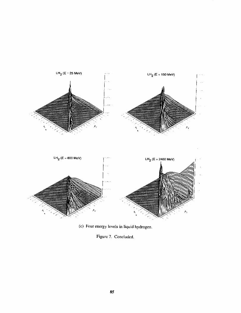
LH 2 (E = 25 MeV)
_,_711.....
LH 2 (E = 150 MeV)
LH 2 (E = 600 MeV) t "
,_' ,'i_,,_' _
LH 2 (E = 2400 MeV)
(c) Four energy levels in liquid hydrogen.
Figure 7. Concluded.
85

106 _-
105
103i
102
lO1¢..q
100
10_1
"_10 -2
lO, t-,_ /..- ,,_', ,, \-= .,/ ..'" ",X', \ \
_:Charge Z _.',_ \; 1- .'¢', "', \
10-3_ ..... 2
_ 3 -<Z< 10 "'" "X "
10 -4 _ • ,11 <_Z_<20 ,,_,
10 -51-1- ...... 21 _<Z<28
10-'61" I I ll1 t I in[ I J ttl i i tll ) t ill t t Itl t I tit
10 -1 100 101 102 103 104 105 106
Energy, A MeV
(a) GCR ion flux for 1977 solar minimum.
10 6 =
105
lO.
_,_ 10 3
_ 10 2
ca<, 101
o 10 0
-_,o-1_-'..<.:._•-',.'\ '\ \-_ _,<-'..-- _z '..-_,,- \lo-2 - ... - .-,,,, ", \_-" ld
!o-3 ..... 2 "'.._,',, ,3_<Z<iO .x_,\ ',
10 -4 11 <Z<20 ,_
...... 21 <Z<28 \10-5 - ,
10 -6 ) I II1 t I tll J I )ll I I ill ) t tll I J ttl t I ill
10 -1 100 101 102 103 104 105 106
Energy, A MeV
(b) GCR ion flux for 1981 solar maximum.
Figure 8. Differential fluence spectra.
86

Figure9.
O
u
100
10-1
f Charge Z
1
..... 2
----- 3 <Z< 10
11 -<Z<20
...... 21 <Z_<28
10-2 J _ _1 _ i _1 _ a l_l i a ill i t ill i i Jtl J i iJl
10 -I 100 101 102 103 104 105 106
Energy, A MeV
GCR ion flux ratio of 1981 solar maximum to 1977 solar minimum.
¢q
...r
A
t-
1011 -
1010
109
i
x
..... No_. 1960 -'\ I,', \
Oct. 1989 i'll ', \
107 i i _Jl _ J _1 _ _1'. J_ _ _1\ , , ,_1
10 -1 10 0 101 10 2 10 3 10 4
Energy, A MeV
108
Figure 10. Integral fluence spectra of important solar particle events.
87

,i
10-2
QE-
10-1 _ 0 HZETRNNTC
10-3 I I t I I I I I I I
0 6 12 18 24 30
Water depth, g/cm 2
t-
O'*
O
[-
!0 0 O HZETRN
I NTC
10-1
10 -2
10 -3 1 I
0
I I I I I I I I I
6 12 18 24 30Water depth, g/cm 2
(a) Aluminum shield on water. 20 g/cm 2 AI; 30 g/cm 2 water.
Figure 11. Total dose and total dose equivalent.
88

@
10-1
10 -2
10-3
0
- © HZETRN
-- NTC
O
%_o
i I J I J I a f
12 18 24 30Water depth, g/era 2
100 _
10-1..gc-
O
_ 10_2
O HZETRN
NTC
10 -3 I I J I I I I I I I
0 6 12 18 24 30
Water depth, g/cm 2
(b) Iron shield on water. 20 g/cm 2 Fe; 30 g/cm 2 water.
Figure 11. Concluded.
89

10-2
lo-3O
0 HZETRN
NTC
_0
10 -4 t I , I I I I I I I
0 6 12 18 24 30Water depth, g/cm 2
]
@
10-1 O HZETRNNTC
10-2
0 0 0 0 !
10-3 i I
0 6
0 0 0 0 00 0
0 0 0
l I I I I I I I
12 18 2 24 30Water depth, g/cm
(a) Aluminum shield on water. 20 g/cm 2 AI; 30 g/cm 2 water.
Figure 12. Secondary neutron dose and dose equivalent.
9O

10 -2 _
10 -30
© HZETRN
NTC
_O
I I I J I I 1 I I
6 12 18 24 30Water depth, g/cm 2
10-1
o
10_2,..,t
0
0 HZETRN
NTC
O
o LO
OO
OO
0 0 0 0
1 o
10 -3 I I I I j I a I I I
0 6 12 18 24 30Water depth, g/cm 2
(b) Iron shield on water. 20 g/cm 2 Fe; 30 g/cm 2 water.
Figure 12. Concluded.
91

103
102
>
< lO1¢-q
•_ 10 0¢-,
10-1
Depth, g/cm 2
0
..... 10
..... 20
,'" 30
_ /
10-2
10-2
n , all n i iii i i l,l I i ill i i ill i I iii i ,'!i,l
10 -1 100 101 102 103 104 105
Energy, A MeV
(a) 1977 solar minimum.
103
10-2
10-2 10 -1 100 101 102
Energy, A MeV
Depth, g/cm 2
0
..... 10
20
30
103 104 105
(b) 1981 solar maximum.
Figure 13. GCR energy flux for carbon ion in aluminum.
92

;>
IO1
E
.6•_ 100
,4
10-1
103
Depth, g/cm 2
0
10102 20
30
10-2 _ , ,,I _ , ,Jl _ J _1 , ,Jtl , J J,I , J _1 _ _.,,1
10 .2 10-1 100 101 102 l03 104 105
Energy, A MeV
(a) 1977 solar minimum.
103
102
;>
<, 101I'M
"6"_ 100
10-1
Depth, g/cm 2
0
..... 10
----- 20
30
t
"1/////
,2"- -- - ";'/"
10-2 J t_,l i a,,I , I Jll , J ,,I , ,J,I t J ,,I I rlll
10 -2 10-1 100 101 102 103 104 105
Energy, A MeV
(b) 1981 solar maximum.
Figure 14. GCR energy flux for oxygen ion in aluminum.
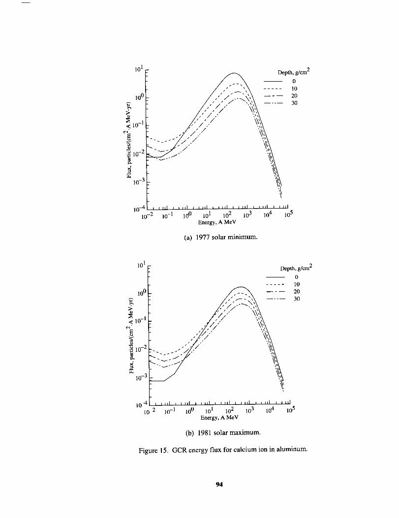
101
lOo
0
10-1
E
•_ 10 .2e_
10-3
10 -4
10 -2
Depth, g/cm 2
0
..... 10
20
30
| J JJl I I III ! ! ill I I Ill l I Ill I ) I_ I I 111
I0 -1 10 0 101 10 2 10 3 10 4 10 5
Energy, A MeV
(a) 1977 solar minimum.
100
10-1
Eo
o
•_ 10 .2
10-3
101 _
1 /
//,,"
Depth, g/cm 2
0
..... 10
20
30
10-4 i ,,ll , i !nl i _l,l t , J,l , _ rill, ii,l i ,ill
10-2 10-1 100 10 i 102 103 104 105
Energy, A MeV
(b) 1981 solar maximum.
Figure 15. GCR energy flux for calcium ion in aluminum.
94

102
101
< 1o°¢.q
._ 10 -1
10-2
10-3
10-2
Depth, g/cm 2
0
..... 10
2O
30
:-- -._-
J n _ll i i ill i I ill J J ill i _ ill f J ill J q'll]
10 -1 100 101 102 103 104 105
Energy, A MeV
(a) 1977 solar minimum.
102
101
<, 100¢,q
"6._ 10 -1
10-2
10-3
10-2
Depth, g/cm 2
0
..... 10
----- 20
30
/
s I
,,\,ill
10 -1 10 0 101 10 2 10 3 10 4 10 5
Energy, A MeV
(b) 1981 solar maximum.
Figure 16. GCR energy flux for iron ion in aluminum.
95

103
102
_ 101
E10 0
"_ 10_ I
10.2
10-3 , i ill i i ill i i ill i illi i i ill t i ill l i ill
10-2 10 -1 100 10 ! 102 103 104 105
Energy, A MeV
Depth, g/crn 2
0
10
20
30
(a) 1977 solar minimum.
103
102
_ 101
<,E
10 0
"_ 10_ !
10 .2
10-3
Depth, g/cm 2
0
..... 10
----- 20
30
i _ i,l i i ,il i , iii i I III I I Ill I I It] I } III
10-2 10-1 100 101 102 103 104 105
Energy, A MeV
(b) 1981 solar maximum.
Figure 17. GCR energy flux for carbon ion in water.
96

10 2
101
100
"6
"_ 10-I
10-2
103 -
',\
\
Depth, g/cm 2
0
10
20
30
10-3 J i III I , Ill , I ,il i JlJl , J Ill i J ,il i , Ill
10-2 10-! 100 101 102 103 104 105
Energy, A MeV
(a) 1977 solar minimum.
103
102
_ 101
<t.,,i _
10 0
"_ 10_ 1
10 -2
I I II1 I I III I I II1 I 1 Ill I I II1 I I II1 I I Ill
10 -1 100 101 102 103 104 105
Energy, A MeV
10-3
10-2
Depth, g/cm 2
0
10
20
30
(b) 1981 solar maximum.
Figure 18. GCR energy flux for oxygen ion in water.
97
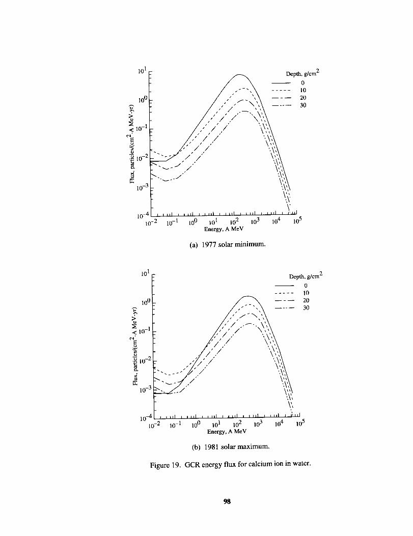
10 o
>
10-1
E
-_ 10 .2
101 _
I10-2 10-1 104 10 5
Depth, g/cm 2
0
10
20
30
100 101 102 103
Energy, A MeV
(a) 1977 solar minimum.
101 _
10 0 /'_
-..... ,/-/ ,,,\,,_
,o_.y.. ":il10--41 , ,,,I i ,,,I ,, ,,I , ,ill i ,,,I , ,,,I i _,sll
10-2 10-1 10 0 101 10 2 10 3 10 4 10 5
Energy, A MeV
Depth, g/cm 2
0
10
20
30
(b) 1981 solar maximum.
Figure 19. GCR energy flux for calcium ion in water.
98

lO 1
>_ 10 0
<i
¢'-I
_10 -1
"_ 10 .2
10-3
102 - Depth, g/cm 2
0
..... 10
20
30
\\
10-4_ I I Ill I ' ,,I .... I , , ,,I .... I .... I , },,,I
10-2 lO-I 10 0 101 102 10 3 10 4 10 5
Energy, A MeV
(a) 1977 solar minimum.
102
101
>o 100
<,t"-I
10 -1
"_ 10 -2
[.r.,
10-3
Depth, g/cm 2
0
..... 10
20
30
_ / \,\,
I I II1 1 J Ill I I II1 1 I Ill I I Ill I I III I Iklll
10-I 100 101 102 103 104 105
Energy, A MeV
(b) 1981 solar maximum.
Figure 20. GCR energy flux for iron ion in water.
99

103_
102
;>o101
¢",1
10 0
_lO-I
u,
10-2
10-3
10-2
Depth, g/cm 2
0
..... 10
20
30
s
'l
\\
I I Ill I i _ll _ I ill I L Ill J _ _ll i t ill I _lal
10 -1 100 101 102 103 104 105
Energy, A MeV
(a) 1977 solar minimum.
103
102 !
>o 101
<¢..1 _
Eu 100
_10-1
K
IT.
10--2
10--3
10--2
\.I I I1[ I I IlL i i liD i i |1[ i I iiI i i iii i i_,lli
10 -1 100 101 102 103 104 105
Energy, A MeV
Depth, g/cm 2
0
10
20
30
(b) 1981 solar maximum.
Figure 21. GCR energy flux for carbon ion in liquid hydrogen.
100

10 3
102
K:; lO1
< lO0eq
"alO -1
lO -2
10-3
10 -4 _ _ ,,I j _J,I
10-2 10-1 10 0
_ Depth, g/cm 2
- 0
10
20
30
.------ /./././ \,,\,',,,\
_-1-/" /" k. \,',,,\
/ \\,,,
-/ \\i
\
I II1 I I I1[ I I II1 I I Ill I I III
101 102 103 104 105
Energy, A MeV
(a) 1977 solar minimum.
103
10 2
1o1
<, 10 0
_ 10 -1
_ 10 .2
10-3
10--4i , J J,I , J,,I , J,_l I i_Jl ,
10 -2 10-1 100 101 10 2
Energy, A MeV
/ \\'/
\I III I I III I IIII
103 104 105
Depth, g/cm 2
0
10
20
30
(b) 1981 solar maximum.
Figure 22. GCR energy flux for oxygen ion in liquid hydrogen.
101

101
10 o
10-1
e_,lO -2
_ 10.3
_ 10 -4
10-5
10-6
10-2
Depth,0g/cm2
..... 10
----- 20
.... 30
z / •
/ / \ \ ',--_-/ / \ \
/ '\ \/"
.... i \
I J II1 I I III I I III I I I|1 I I II1 I I Ill I _1 Ill
10 -1 100 101 102 103 104 105
Energy, A MeV
(a) 1977 solar minimum.
101
10 o
10-1
,10-2
"d 10 .3
e._
-4
10-5
Depth, g/cm 2
0
10
20
30
/i
/
/
/ \
/ \
\
\
/" \10-6 ",'-,-._r', ,,,I , i,,l i l lll , i,,l i ,t,l p',, ,,I
10-2 10 -1 100 101 102 103 104 105
Energy, A MeV
(b) 1981 solar maximum.
Figure 23. GCR energy flux for calcium ion in liquid hydrogen.
102

102
101
100
_,_10 -1>o
10-2<
10-3o
_ 10--4
"_ 10-5e_
10 _5
10-7
10-8
10-9 i
10 -2
_ _sl • -_
J
Depth, g/cm 2
0
10
20
x
/ \ ',j
- \J
J j
j" \
j- \
30
i Ill I I I11 I I ltl I I III i i III I i 111 I i Ill
10-1 100 101 102 103 104 105
Energy. A MeV
(a) 1977 solar minimum.
102
101
.-. 100
;_10 -1
10-2
_'E 10-3
_-_10 -4c.J
_ 10 -5
_10-6
Depth, g/cm 2
0
- 10
- 20
30
.- J \
.JJ f - - "---_
10 -7 .._
10-8 >-._.-/_
10-9 J , J,I , , ,,I , J JJl J , JJl , , ,,I J
10-2 10-1 10 0 101 10 2 10 3
Energy, A MeV
xx
x
\
\x
\
\
\
i ill i n Ill
104 105
(b) 1981 solar maximum.
Figure 24. GCR energy flux for iron ion in liquid hydrogen.
103

i0 o
1o-1_3
10-2
0
1977 solar min.
..... 1981, 1982 solar max.
l I i I i I L I ,
6 12 18 24
Shield depth, g/cm 2
I
30
,,.$
@
101
10 o
10-1
10-2
1977 solar min.
..... 1981, 1982 solar max.
t I i I J I i I t I
6 12 18 24 30
Shield depth, g/cm 2
Figure 25.
(a) In aluminum.
GCR skin dose and dose equivalent.
104

o£O
10o
10-1
10-2
0
1977 solar rain.
..... 1981, 1982 solar max.
J I I I I I i I t I
6 12 18 24 30Shield depth, g/cm 2
O
t_
101 _
100
10 -1
10-2
1977 solar min.
..... 1981, 1982 solar max.
f I J I J I i I 1 I
6 12 18 24 30Shield depth, g/cm 2
(b) In water.
Figure 25. Continued.
105

10 o
1o-1O
10-2
0
1977 solar min,
..... 1981, 1982 solar max.
K I i I I I t I i I
6 12 18 2 24 30Shield depth, g/cm
¢0
¢P_J
0
101
100
10-1
10-2
I 1977 solar rain.
..... 1981, 1982 solar max,
i I I I i I s I e I
0 6 12 18 24 30Shield depth, g/cm 2
(c) In liquid hydrogen.
Figure 25. Concluded.
106

O
r_
101 _
10 o
10-1
10-2
0
AI
..... H20
LH 2
---,..,..
I i I J I I I t I
6 12 18 24 30Shield depth, g/cm 2
e-
101 _
100
10-1
10-2
0
AI
..... H20
_____ LH 2
I I I I I I I N I
6 12 18 2 24 30Shield depth, g/cm
(a) 1977 solar minimum.
Figure 26. GCR skin dose and dose equivalent in aluminum, water, and liquid hydrogen.
107

101-
10 0
i0 -1
10-2
0
A!
..... H20
_____ LH 2
I I t I i I t I I I
6 12 18 2 24 30Shield depth, g/cm
101 -
10 0
-._
0
_ 10-1
10-20
\
AI
..... H20
__ _ __ LH 2
I I I I I
6 12 18 2Shield depth, g/cm
I I I
24 30
(b) 1981 solar maximum.
Figure 26. Concluded.
108

100
0
10-1
10-2
10-3
10-4
10-50
I t I I I I I t I
6 12 18 24 30
Shield depth, g/cm 2
(a) 1977 solar minimum.
Charge Z
0
1
2
3 -<Z< 10
11 <Z<20
21 <Z<28
10 0 -
@
10-1
10-2
10-3
10-4
10-5
____ ...........................
_2£_L S 22 "
J
fI I t
6I J I I I I I
12 18 24 30
Shield depth, g/cm 2
Charge Z
0
1
2
3<Z_<I0
11 _<Z_<20
21 <Z<28
(b) 1981 solar maximum.
Figure 27. GCR skin dose for six charge Z groups in aluminum.
109

100
10 -1
10 -2
10-3
10 -4
10-5
0
Ja l i
6
I. t I I I
12 18 24
Shield depth, g/cm 2
I
30
(a) 1977 solar minimum.
Charge Z
0
1
2
3 <Z< 10
11 <Z_<20
21 <Z<28
i0 o
10-1
10-2
@
10-3
10-4
10-5
0
_.____._ ..........................
=-"-_7.
6
I I i I J I i I
12 18 24 30
Shield depth, g/cm 2
(b) 1981 solar maximum.
Figure 28. GCR skin dose for six charge Z groups in water.
Charge Z
0
1
2
3<Z_< 10
11 <Z<20
21 <Z<28
110

C,
10-1 _ .................................
10- - \ ",. "'-_ --_..
10-3
10-4
\
\
\
\
\
k
\
\
\
\
,..
\
I i I i I J\ I i I
6 12 18 24 30
Shield depth, g/era 2
10-5 i
0
(a) 1977 solar minimum.
Charge Z
0
1
2
3 <Z< 10
11 <Z<20
21 -<Z_<28
10-1
0
10-2
10-3
10-4
10 -5 J I
0 6
N
\
\
N
N
\ "•
\ ".,
\
\
\
\
I \ I I
12 18 24
Shield depth, g/cm 2
i I
30
Charge Z
0..... ]
2
3_<Z_<lO
...... ll_<Z_<20
21 <Z_<28
(b) 1981 solar maximum.
Figure 29. GCR skin dose for six charge Z groups in liquid hydrogen.
111

100 -
10-1 _ _ ¢-. _ ----.-
(I]
10 -2
"3
N 10 .3@
10--4
Charge Z
0
..... 1
2
3<Z<IO
...... 11 <Z<-20
21 <Z<28
10-5 I I i I i I I I I I0 6 12 18 24 30
Shield depth, g/cm 2
(a) 1977 solar minimum.
Figure 30.
100
"V-" -':'-'" _ _-- "-- ..........
10 -2
•_ Charge Z
N 10_ 3 0..... 1
23<_Z_<IO
!0--4 kJ 11 -<Z< 2021 <_Z<28
10 .5 I i I t I t I I I t I0 6 12 18 24 30
Shield depth, g/cm 2
(b) 1981 solar maximum.
GCR skin dose equivalent for six charge Z groups in aluminum.
112

10 o
10 -1
oO
lO-2
N 10.3@
10-4
10-51
0
i
I
- c I
Charge Z
0
1
2
3 <Z< 10
I1 <Z<20
21 <Z_<28
I i I I I i I I I
6 12 18 24 30
Shield depth, g/cm 2
(a) 1977 solar minimum.
10o
10-1
_ 10.2e-,
"3
N 10 .30
10--4
10-5
0
Figure 31.
.............
Charge Z0
..... 1
2
3_<Z_< 10
...... 11 <Z_<20
21 <Z<28
i I I J I J I I I I
6 12 ! 8 24 30
Shield depth, g/cm 2
(b) 1981 solar maximum.
GCR skin dose equivalent for six charge Z groups in water.
113

10 0
10-1
lO-2o
m
gN 10 -3O
10--4
.... __ ......
-__-" z._ "_--
\
10 -5 I I i I i I
0 6 12 18
Shield depth, g/cm 2
\
\
\
\
\
\
\
\
i I _ "1
24 30
(a) 1977 solar minimum.
Charge Z
0
1
2
3 <Z< I0
11 <Z<20
21 _<Z<28
_10-3@
10o
10 -1 .I", .x ,,,"\'.
o_ .- . _ .-... - ..........10 -2 "---- ----. ----- _ \_ -.-,_,
\
10 -4
\
\
\
\
i I
6
\
\
N.
\
10 -5 1 I t 1 l I i
0 12 18 24
Shield depth, g/cm 2
\
\1
30
Charge Z
0
1
2
3<Z<IO
11 <Z_<20
21 <Z<28
(b) 1981 solar maximum.
Figure 32. GCR skin dose equivalent for six charge Z groups in liquid hydrogen.
114

I0 0
lO-I©
10-20
1977 solar rain.
..... 1981, 1982 solar max.
i I J I i I t I i
6 12 18 _ 24Shield depth, g/cm 2
I
3O
.5
o
101 _
10o
10-1
10-2
1977 solar min.
..... 1981, 1982 solar max.
I I I I i I i I i I
0 6 12 18 24 30Shield depth, g/cm 2
Figure 33.
(a) In aluminum.
GCR 5-cm-BFO dose and dose equivalent.
115

O
¢2
10 0 -
10 -1
10-2
0
1977 solar rain.
..... 1981, 1982 solar max.
i I t I i I
12 18 2 24Shield depth, g/cm
I
30
101
_. !00ra_
0"
_ 10-1
10 -2 I I
0 6
1977 solar min.
..... 1981, 1982 solar max.
I L I i I i I
12 18 24 302
Shield depth, g/cm
(b) In water.
Figure 33. Continued.
116

10o
m-1@
t_
10 -2
0
1977 solar min.
..... 1981, 1982 solar max.
J I t I i I t I
6 12 18 24
Shield depth, g/cm 2
I
30
101
> 10 0
°_
@
t21 10-1
10-2_
1977 solar min.
..... 1981, 1982 solar max.
I J I I I i I i I
6 12 18 24 30Shield depth, g/cm 2
(c) In liquid hydrogen.
Figure 33. Concluded.
117

@
101
100
10 -1
AI
..... H20
LH 2
10-2 I I I I i I i I J I
0 6 12 18 2 24 30Shield depth, g/cm
101 A1
I ..... H20
----- LH 2
10 0
10 -1
10 -2
0
I I I I I I I I I
12 18 24 306 Shield depth, g/cm 2
(a) 1977 solar minimum.
Figure 34. GCR 5-cm-BFO dose and dose equivalent in aluminum, water, and liquid hydrogen.
118

O
101
10 o
10 -1
10-2i
0
AI
..... H20
__ _ __ LH 2
-.-......
i I i I i I i I
12 18 24 30Shield depth, g/cm 2
101 _
_, 100
..>Q,,
0
_ 10-1
10-2
0
A1
..... H20
__ _ __ LH 2
I I I I I I I I I I
6 12 18 2 24 30Shield depth, g/cm
(b) 1981 solar maximum.
Figure 34. Concluded.
119

10o
10-I
10-2
10-3
10 -4
10-5
0
...................................
_ 2212
I I I I I I i I t J
6 12 18 24 30
Shield depth, g/cm 2
(a) 1977 solar minimum.
Charge Z
0
1
2
3 <Z< 10
11 <Z<_20
21 <Z_<28
100
O
10-I
10-2
10-3
10-4
10-5
Charge Z
0
1
2
3 <Z<_ 10
11 <Z<20
21 <Z_<28
J I J I m I I I i I
0 6 12 18 24 30
Shield depth, g/cm 2
Figure 35.
(b) 1981 solar maximum.
GCR 5-cm-BFO dose for six charge Z groups in aluminum.
120

10 o
10 -1
10-2 i
0
_ 10-3
10 -4
10-5
0
t 1 _ I I I I I _ I
6 12 18 24 30
Shield depth, g/cm 2
(a) 1977 solar minimum.
Charge Z
0
1
2
3<Z<10
11 <Z<20
21 <Z<28
10 0 -
0
10-1
10-2
10-3
10-4
10-5
" - Charge Z
"_ . 0
..... |
----- 2
3<_Z<_IO
...... 11 _<Z_<20
21 _<Z_<28
_
i I i I J 1 J I J I
0 6 12 18 24 30
Shield depth, g/cm 2
(b) 1981 solar maximum.
Figure 36. GCR 5-cm-BFO dose for six charge Z groups in water.
121

10 0
C,
I0-1
10-2
10-3
10--4
\
\ ". ,
\ • ,
\ ".
10 -5 J 1 I
0 6
\
\ ".
\I I I ,_A I I I
12 18 24 30
Shield depth, g/cm 2
(a) 1977 solar minimum.
Charge Z
0
1
2
3<Z<lO
11 <-Z<20
21 <Z<28
100
10-1
10-2
10-3
10-4
10-50
Figure 37.
\
\ - , --o
\ .
\ ".
\
,N, , , .
\\h ""I i I t A I i "-I
6 12 18 24 30
Shield depth, g/cm 2
Charge Z
0
1
2
3 <Z< 10
11 <Z<20
21 <Z_<28
(b) 1981 solar maximum.
GCR 5-cm-BFO dose for six charge Z groups in liquid hydrogen.
122

10 0 _
_. 10 -1
.,..r
o
_ 10-2
10-3
0
:--:':-7::%[--- - ...................
_...¢_ ..-- . .
""_ ,_...
I I I I i I J I i I
6 12 18 24 30Shield depth, g/cm 2
(a) 1977 solar minimum.
---h
Charge Z
0
1
2
3 <Z< 10
11 -<Z_< 20
21 -<Z<28
10 0 _
._>
t2r
@
10-1
10-2
- . . . . .
_- :._ _________ _ -.--
10-3 f I I I
0 24 30
/
I I I I I I
6 12 18 2Shield depth, g/cm
Charge Z
0
1
2
3 _<Z< 10
11 -<Z<20
21 <Z<28
(b) 1981 solar maximum.
Figure 38. GCR 5-cm-BFO dose equivalent for six charge Z groups in aluminum.
123

10 0
_, 10 -1
ID
::1
E
_ 10-2
10-3
0
1
_--. _--._-. ---_ 2"-... "-_ . . 3_<Z<IO
•.. ...... 11 -<Z<20
21 _<Z_< 28
i I i I J I J I i I
6 12 18 24 30Shield depth, g/cm 2
(a) 1977 solar minimum.
10 o
_. 10 -1
10 -2
Charge Z
e_. " - . • 0
_ " . 3_<Z_<IO
.__ -_ . ..... II _<Z<_2021 _<Z<_28
J
10 -3 I I I I I I I I t I0 6 12 18 24 30
Shield depth, g/cm 2
(b) 1981 solar maximum.
Figure 39. GCR 5-cm-BFO dose equivalent for six charge Z groups in water.
12,4

100 I' -
\-. ...........................
"5 10-2 \ "'". "'_-N
10-3
10 .--4 A I J
0 6
O
\\
\
\
I i
12
• ",,
\
\ -
\ "
\
I J\ I i I
18 24 30
Shield depth, g/era 2
(a) 1977 solar minimum.
Charge Z
0
1
2
3_<Z<lO
11 _<Z< 20
21 <Z<28
10 o
10-1
r._
J
•5 10 -2
O
10-3
.\
::
\ ". _..
"''', ...
\
\
N
\
\ •
t I L I i I "h I t "'1
6 12 18 24 30
Shield depth, g/cm 2
Charge Z
0
1
2
3 <Z< 10
lI<Z<20
21 <Z<28
(b) 1981 solar maximum.
Figure 40. GCR 5-cm-BFO dose equivalent for six charge Z groups in liquid hydrogen.
125

"7
t'q
¢
109
108
107
106
105
lo4
103
102
100 101
\
\
102 103
LET, (MeV-cm2)/g
10 4
(a) 1977 solar minimum.
Depth, g/cm 2
0
..... i0
20
30
105
-7
t",l
,_J
109
108
107
106
105
1o4
Depth, g/cm 2
0
..... 10
_--- 20
30
103
100 101 102 103 104 105
LET, (MeV-cm2)/g
(b) 1981 solar maximum.
Figure 41. GCR skin integral flux LET spectra in aluminum.
126
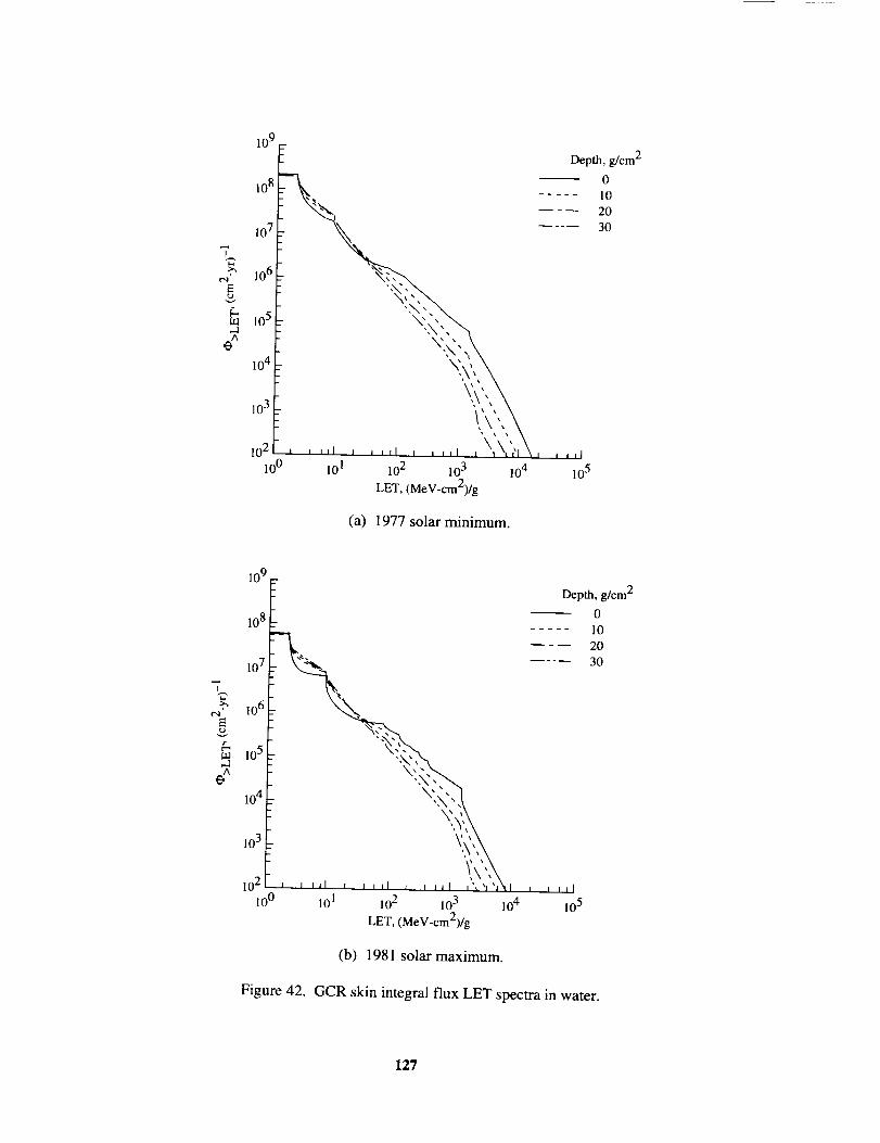
.7"2"
¢q
E
g,-3A
109
108
107
106
105
104
103
102
10 o 101 102 103 104
LET, (MeV-cm2)/g
(a) 1977 solar minimum.
Depth, g/cm 2
0
..... 10
----- 20
30
105
"7
t'q
g.LO.3A
e
109
108 I
107_ "_z-._,. _.106 •
105
o4:_
-10 2 J , Ill I i III 1 t ill i\xlxa_tl
I00 101 102 103 104
LET, (MeV-cm2)/g
Depth, g/cm 2
0
..... 10
----- 20
30
I I Ill
105
(b) 1981 solar maximum.
Figure 42. GCR skin integral flux LET spectra in water.
127

"7
.d
109
108
107
106
105
104
103
102
10 o 101 102 103
LET, (MeV-cm2)/g
104
(a) 1977 solar minimum.
Depth, g/cm 2
0
..... 10
20
30
105
"7
t"q
E
G
Ae
109
108
107
106
105
104
103
102
100
, ..,, , ... , ',,,\101 102 103 104
LET, (MeV-cm2)/g
Depth, g/cm 2
0
..... 10
20
30
i I11
10 5
(b) 1981 solar maximum.
Figure 43. GCR skin integral flux LET spectra in liquid hydrogen.
128
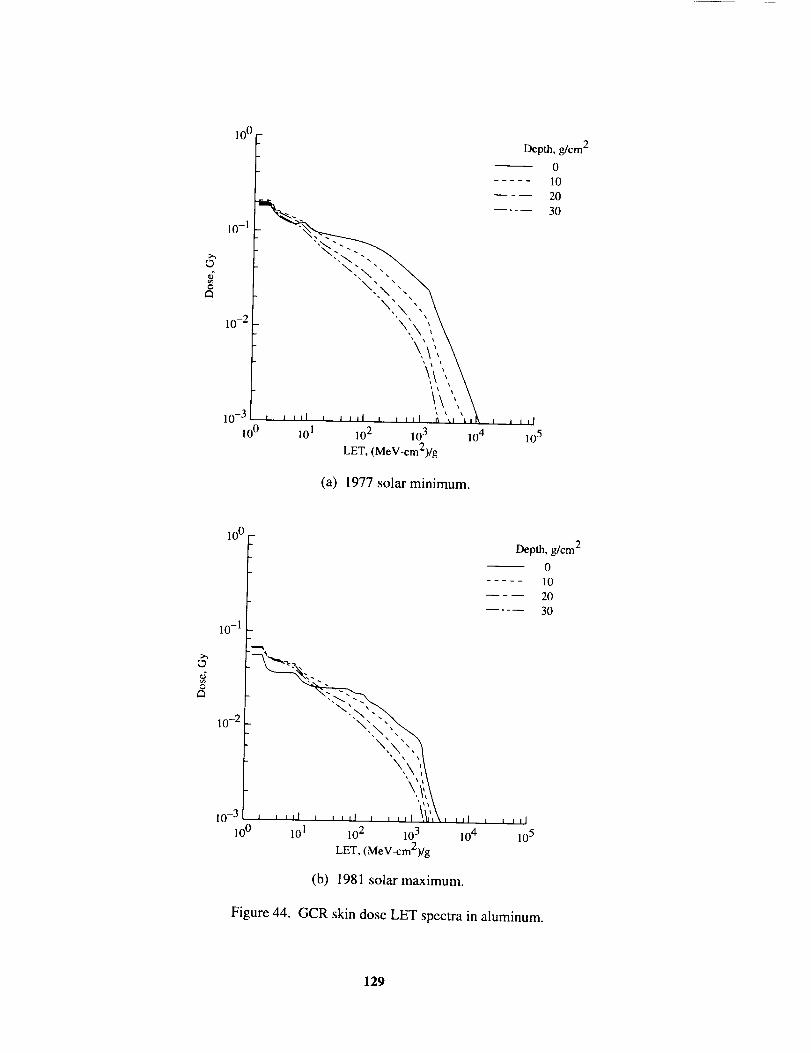
D
O
10-1
10-2
10-3
10 o
,°°I
'\ \', \
}:ii,101 102 103 104
LET, (MeV-cm2)/g
(a) 1977 solar minimum.
Depth, g/cm 2
0
..... 10
----- 20
30
i i Ill
105
@
10 o
10-1
10 3I "\:fi"\
100 101 102 103
LET, (MeV-cm2)/g
_,1
104
(b) 1981 solar maximum.
Depth, g/cm 2
0
..... 10
----- 20
30
Figure 44. GCR skin dose LET spectra in aluminum.
129
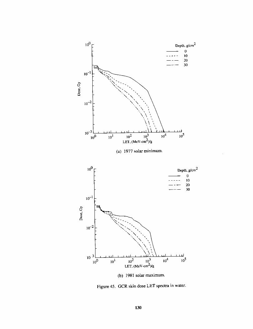
10 o
10-1
10-2
10-3
100 101 10 2 10 3 10 4
LET, (MeV-cm2)/g
(a) 1977 solar minimum.
Depth, g/cm 2
0
..... 10
----- 20
30
J I ItJ
10 5
1o0 _-
o
10-1
10-2
10-3
100
\.', ",\
101 10 2 10 3
LET, (MeV-cm2)/g
Ill
104
(b) 1981 solar maximum.
Depth, g/cm 2
0
..... 10
20
30
Figure 45. GCR skin dose LET spectra in water.
130

_2@
t_
i0 0
i0-I
10 -2
10-3
10o
\ \ ", \
101 102 103 104
LET, (MeV-cm2)/g
(a) 1977 solar minimum.
Depth, g/cm 2
0
..... 10
20
30
I I I II
105
@
10 o
i0-I
10-2
10-3
I0 0
',.?,, "',,, \'_. \.., "'. , .\
) i ,,l",, ,"),,I t ,',,1 ,\
101 10 2 10 3
LET, (MeV-cm2)/g
Depth, g/cm 2
0
..... 10
20
30
104 105
(b) 1981 solar maximum.
Figure 46. GCR skin dose LET spectra in liquid hydrogen.
131

O')
t_cO
"2
101 [-
100
10-3
30-2
100
Depth, g/cm 2
0
10
20
30
-_-Z-.
.,?:, \
101 302 103 104
LET, (MeV-cm2)/g
(a) 1977 solar minimum.
_D
_D
@
101 -
300
Depth, g/cm 2
0
..... 10
20
30
10-I
I
\\',,\10 -2 [ I R iI , , IiI , J J II 'J\\_ J II
300 103 102 103 104
LET, (MeV-cm2)/g
(b) 1981 solar maximum.
Figure 47. GCR skin dose equivalent LET spectra in aluminum.
132

101
10-2
10 o
;_ 10 0
..a
13"
O
_ 10-1
Depth, g/cm 2
0
..... 10
----- 20
30
...... '--(5,:,\
, ,,,, , ,,,, , ,,,, ",2\':,,,_,101 10 2 10 3 10 4
LET, (MeV-cm2)/g
(a) 1977 solar minimum.
_r
.2-i
O
r_
101
10 o
Depth, g/cm 2
0
..... 10
----- 20
30
10-1 --12\2-g;-----
100 101 102 103 104
LET, (MeV-cm2)/g
(b) 1981 solar maximum.
Figure 48. GCR skin dose equivalent LET spectra in water.
133

..r
o
o"
@
_2
101
10 0
10-1
10-2
10 -3 I
10 o
Depth, g/cm 2
0
..... 10
20
30
• _ x x
"\.. _. ', \
- \
\ \ ',I I II t I I II I I 'r II _ I. I _1 II
101 10 2 10 3 10 4
LET, (MeV-cm2)/g
(a) 1977 solar minimum.
.,..r
o
_r8
101
100
10-1
10-2
10-3
100
Depth, g/cm 2
0
..... 10
----- 20
30
_ \ -\ ', \
_ "\ ', \
1 I , 11 I , I"'__ I I ii_l I", I I
101 102 103 104
LET, (MeV-cm2)/g
(b) 1981 solar maximum.
Figure 49. GCR skin dose equivalent LET spectra in liquid hydrogen.
134

10 9
10 8
10 7
"7
_,_ 10 6E
o
g-10 5
....3
10 4
10 3
10 2
10 0 101 102 103
LET, (MeV-cm2)/g
10 4
(a) 1977 solar minimum.
Depth, g/cm 2
0
..... 10
20
30
105
10 9
10 8
10 7
"7
_,_ 10 6
105
A
10 4
Depth, g/cm 2
0
..... 10
----- 20
30
10 3
10 2
10 o
Figure 50.
101 102 103 104 105
LET, (MeV-cm2)/g
(b) 1981 solar maximum.
GCR 5-cm-BFO integral flux LET spectra in aluminum.
135

10 9
10 8
10 7
"7
_ 10 6
&
_105
e
lO 4
lo3 x,_,,,\,02 _, , ,,,, ,'_x',",\, ,,,'
100 101 102 103 104 105
LET, (MeV-cm2)/g
Depth,_cm 2
0
..... 10
20
30
(a) 1977 solar minimum.
109
108
-_._ -- _ _
107
104 1 '_x_',_k
102[ - _l , i ,ll , i i,I I',I,,X,I , t J ,1
100 101 102 103 104 105
LET, (MeV-cm2)/g
Depth, g/cm 2
0
10
20
30
(b) 1981 solar maximum.
Figure 51. GCR 5-cm-BFO integral flux LET spectra in water.
136

10 9
10 8'
10 7
_,_ 10 6E
_105,dA
e
10 4
103
102
100
Depth, g/crn 2
0
..... 10
_X,, 20
_. 30
X\', \
I I I I I I 1 I II I I I _ I i II
101 102 103 104 105
LET, (MeV-cm2)/g
(a) 1977 solar minimum.
10 9
10 8
107
_,_ 10 6
105A
e
10 4
103
10 0 101 10 2 10 3 104 10 5
LET, (MeV-cm2)/g
Depth, g/cm 2
0
..... 10
20
30
(b) 1981 solar maximum.
Figure 52. GCR 5-cm-BFO integral flux LET spectra in liquid hydrogen.
137

10 0
10-1
10-2
Depth, g/cm 2
0
..... 10
----- 20
30
,\,
\\,,'\'\ ,,
10-3
100 101 102 103 104
LET, (MeV-cm2)/g
(a) 1977 solar minimum.
O
100
10-1
10-2
10-3I I I [
10 0 10 4101 102 103
LET, (MeV-cm2)/g
Depth, g/cm 2
0
..... I0
----- 20
30
(b) 1981 solar maximum.
Figure 53. GCR 5-cm-BFO dose LET spectra in aluminum.
138

i0o
10-1
10-2
10-3100 101 102 103 104
LET,(MeV-cm2)/g
(a) 1977solarminimum.
Depth,g/cm20
..... 10203O
100-
10-1
10-2
Depth,g/cm20
..... 102030
"'_-.._ . ..\.'-_ .
"\'\ "-.
10-3 , _ 11 , , , ,I , ,_,lx"k'_. _ , ,I
100 101 102 103 104
LET, (MeV-cra2)/g
(b) 1981 solar maximum.
Figure 54. GCR 5-cm-BFO dose LET spectra in water.
139

L9
@
10 0
10-1
10-2
10-3
10 0
Depth, g/cm 2
0
..... 10
20
\,,_,\ ",,,,,,,,, ,\,101 10 2 10 3 104
LET, (MeV-cm2)/g
(a) 1977 solar minimum.
10 o
10-1
L_
O
10-2
10-3
10o
Figure 55.
Depth, g/cm 2
0
..... 10
----- 20
30
"'\"\\'""'",I , il , , \',,'I. "x ,'h,l \,_
101 102 103
LET, (MeV-cm2)/g
, ill
10 4
(b) 1981 solar maximum.
GCR 5-cm-BFO dose LET spectra in liquid hydrogen.
140

e_
001F_ Depth, g/cm 2/
....... ....- '°°r-,._----__ ........ --. \ ---2o
... -____.....\-.. _ ..... 30
iI,
10 -2 _ , _ ,I , , , ,I , II
100 101 102 103 104
LET, (MeV-cm2)/g
(a) 1977 solar minimum.
>
=
_a
1o 0
10 -1
Dep_,g/cm 2
0
..... 10
----- 20
30
_--LZ ....
|0 -2 I , I II I I , I I i I I I' I1\11_' I [ I I
100 101 102 103 104
LET, (MeV-cm2)/g
(b) 1981 solar maximum.
Figure 56. GCR 5-cm-BFO dose equivalent LET spectra in aluminum.
141

"d
O
10 o
10-1
10 -2
10 0 101 102 103 104
LET, (MeV-cm2)/g
Dep_,_cm 2
0
10
20
30
(a) 1977 solar minimum.
10 0
r_
0
10-2
10 o
Figure 57.
Depth, g/cm 2
0
..... 10
----- 20
30
-.\,N
101 102 103 104
LET, (MeV-cm2)/g
(b) 1981 solar maximum.
GCR 5-cm-BFO dose equivalent LET spectra in water.
142

o_
Q
10 o
10-1
10-2
100
x x
101 10 2 10 3 10 4
LET, (MeV-cm2)/g
Depth, g/cm 2
0
10
20
30
(a) 1977 solar minimum.
O
100 -
10-1
Depth, g/cm 2
0
..... 10
_--- 20
30
\x
--i\.
\ - \
10 -2 I I I ]1 t t 3-. t
100 101 102 103 104
LET, (MeV-cm2)/g
(b) 1981 solar maximum.
Figure 58. GCR 5-cm-BFO dose equivalent LET spectra in liquid hydrogen.
143

Form ApprovedREPORT DOCUMENTATION PAGE oMeno.ozo4-o_ss
Public reporting bur0en for this. collection of infocmation is estimated to average 1 hour per response, including ti_ time for reviewing instrucbon8, searching existing data sources,
gathering and maintaining the data neeOe¢l, and completing anti revmwing the collection of information. Send comments regarding this burden estimate or any other aspect of this
collection of information, including suggestions fo¢ reducing this burden, to Washington Headquallers Services, Directorate fer Information Operations and Reports, 1215 Jefferson
Davis Highway, Suite 1204, Arlington, VA 22202-4302, and to tt_e Office of Managemenl and BuOget, Papen_ork Reductioct Project (0704-0188), Washington, DC 20603.,i
1. AGENCY USE ONLY (Leave blank) 2. REPORT DATE 3. REPORT TYPE AND DATES COVERED
May 1995 Technical Paper4. TITLE AND SUBTITLE 5. FUNDING NUMBERS
HZETRN: Description of a Free-Space Ion and Nucleon Transport andShielding Computer Program WU 199-45-16-11
6. AUTHOR(S)
John W. Wilson, Francis F. Badavi, Francis A. Cucinotta, Judy L. Shirm,Gautarn D. Badhwar, R. Silberberg, C. H. Tsao, Lawrence W. Townsend,and Ram K. Tdpathi
7. PERFORMING ORGAI_IZATION NAME(SI AND ADDRESS(ES)
NASA Langley Research CenterHampton, VA 23681-0001
i
9. SPONSORIING/MONITORING AGENCY NAME(S) AND ADDRESS(F.S)
National Aeronautics and Space AdministrationWashington, DC 20546-0001
8. PERFORMING ORGANIZA'nONREPORT NUMBER
L-17417
10. SPONSORING/MONITORINGAGENCY REPORT NUMBER
NASA TP-3495
11. SUPPLEMENTARY NOTES
Wilson, Cucinotta, Shirm, and Townsend: Langley Research Center, Hampton, VA; Badavi and Tripathi: Christopher NewportUniversity, Newport News, VA; Badhwar: Johnson Space Center, Houston, TX; Silberberg: Universities Space Research Asso-ciation, Washington, D.C.; Tsao: Naval Research Laboratory, Washington, D.C. Software and documentation are available asLAR-15225 through COSMIC, 382 E. Broad Street, University of Georgia, Athens, GA 30602.
12a. DISTRIBUTION/AVAILABILITY STATEMENT 12b. DISTRIBUTION CODE
Unclassified-Unlimited
Subject Category 93Availability: NASA CASI (301) 621-0390
13. ABSTRACT (Maximum 200 words)
The high-charge-and-energy (HZE) transport computer program HZETRN is developed to address the problems offree-space radiation transport and shielding. The I-IZETRN program is intended specifically for the design engineerwho is interested in obtaining fast and accurate dosimetric information for the design and construction of spacemodules and devices. The program is based on a one-dimensional space-marching formulation of the Boltzmarmtransport equation with a straight-ahead approximation. The effect of the long-range Coulomb force and electroninteraction is treated as a continuous slowing-down process. Atomic (electronic) stopping power coefficients withenergies above a few A MeV are calculated by using Bethe's theory including Bragg's rule, Ziegler's shell correc-tions, and effective charge. Nuclear absorption cross sections are obtained from fits to quantum calculations andtotal cross sections are obtained with a Ramsauer formalism. Nuclear fragmentation cross sections are calculatedwith a semiempirical abrasion-ablation fragmentation model. The relation of the final computer code to theBoltzmann equation is discussed in the context of simplifying assumptions. A detailed description of the flow ofthe computer code, input requirements, sample output, and compatibility requirements for non-VAX platforms areprovided.
_14.SUBJECT TERMS
Space radiation; Heavy ions; Shielding
i
17. SECURITY CLASSIFICATIONOF REPORT
Unclassified
NSN 7540-01-280-5500
18. SECURITY CLASSIFICATIONOF THIS PAGE
Unclassified
19. SECURITY CLASSIFICATIONOF ABSTRACT
Unclassified
15. NUMBER OF PAGES
14616. PRICE CODE
A07
20. LIMITATIONOF ABSTRACT
Standard Form 298 (Rev. 2-89)Prescribed by ANSI Std. Z39-15
298-102


National Aeronautics andSpace Administration
Langley Research CenterMail Code 180Hampton, VA 23681-0001
Official Business
Penalty for Private Use, $300
SPECIAL FOURTH-CLASS RATE
POSTAGE & FEES PAID
NASA
Permit No. G-27