Hypothesis TestingHypothesis Testing Hypothesis TestingHypothesis Testing

Topic 11Topic 11

Hypothesis Testing

•Another way of looking at statistical inference in which we want to ask a question like:

•“Is the mean glucose level of infants small-for-gestational age (SGA) the same as those for normal infants?”

i.e. SGA = normal ?

Hypothesis Testing•“Is the mean systolic blood pressure of people taking calcium supplement the same as those in the general population?”

i.e. calcium = gen ?

•“Is the mean systolic pulse rate of people taking a stress test the same as those in the control group?”

i.e. stress = control ?

Null and alternative hypothesis

Null Hypothesis H0 is usually a statement of no effect or no difference. The aim of testing is to assess the strength of evidence presented in the data against the null hypothesis.

Alternative Hypothesis H1 is the hypothesis that we hope or suspect to be true instead of H0 in order to demonstrate the presence of some physical phenomenon or the usefulness of a treatment (e.g., new drug better than old)

Asymmetric treatment of H0 and H1

• H0 is usually the more conservative hypothesis (no change, no effect, etc) which is assumed to be true until sufficient evidence is obtained to warrant its rejection

• H1 is usually the scientifically more interesting hypothesis that we hope or suspect is true (e.g., new drug better than existing drug, smokers more at risk)

• The burden of proof is placed on H1. Substantial supporting evidence is required before it will be accepted

• The consequence of wrongly rejecting H0 (Type I error) is considered more severe than that of wrongly accepting H0 (Type II error)

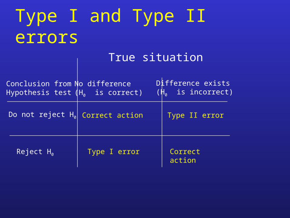
Type I and Type II errors

Type I error

Correct action

Correct action

Type II error

No difference(H0 is correct)

Difference exists(H0 is incorrect)

True situation

Conclusion fromHypothesis test

Do not reject H0

Reject H0

An analogy

Patient

Diagnostic Test Has disease No disease

Tested positive Correct Type II error

Tested negative Type I error Correct

Another analogy

Defendant

Verdict of jury Innocent Guilty

Not guilty Correct Type II error

Guilty Type I error Correct

The 4 steps to hypothesis testing1. Formulate Ho and H1.2. Select an appropriate test statistic which is usually some

kind of standardized difference between the estimated and hypothesized value or between the expected and observed.

3. Use the null distribution (the sampling distribution of the test statistic under Ho ) to calculate the probability due to chance alone of getting a difference larger than or equal to that actually observed in the data. This probability is called the p-value.

4. Draw the appropriate conclusion in the context of the medical problem

Note: A small p-value means it is difficult to attribute the observed difference to chance alone and this can be taken as evidence against the null hypothesis of no difference.

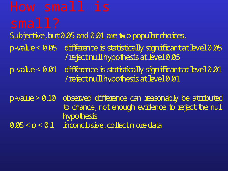
How small is small?Subjective, but 0.05 and 0.01 are two popular choices.

p-value < 0.05 difference is statistically significant at level 0.05/ reject null hypothesis at level 0.05

p-value < 0.01 difference is statistically significant at level 0.01/ reject null hypothesis at level 0.01

p-value > 0.10 observed difference can reasonably be attributedto chance, not enough evidence to reject the nullhypothesis

0.05 < p < 0.1 inconclusive, collect more data

• Some people prefer to report the p-value rather than using terms like “accept/reject” the hypothesis at level 0.05.

• The acceptance/rejection rule is too rigid and exaggerate the difference between, say, p-value = 0.049 and 0.051.

• More informative to report the p-value. Suppose we are told that Ho is rejected at level 0.05, we wouldn’t know whether Ho will still be rejected at level 0.01. The p-value gives us the whole story, e.g., if p-value = 0.012, then we know the hypothesis will be rejected at level 0.05, 0.02 but not 0.01.

Birthweight example revisited•Suppose a random sample of 50 Malay male livebirths gave a sample mean birthweight of 3.55kg and a sample standard deviation of 0.92 kg.

•Question of interest: What is the likelihood that the mean birth-weight from the sampled population (ie all Malay male livebirths) is the same as the mean birth-weight of all male livebirths in the general population which is known to be 3.27kg, after taking into consideration sampling error?

2. Define and compute test statistic

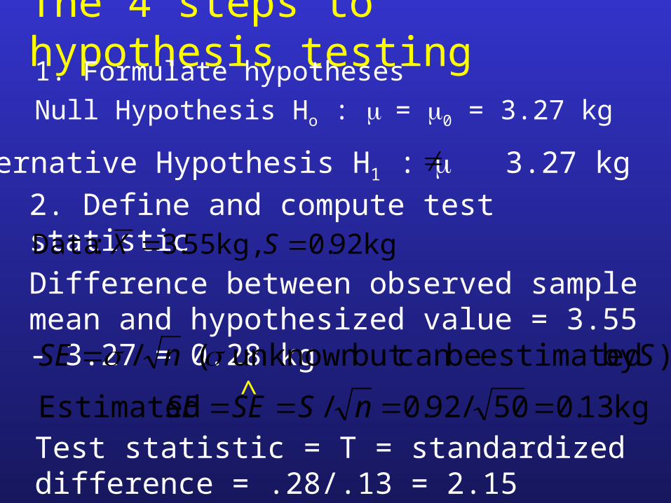
The 4 steps to hypothesis testing1. Formulate hypotheses

Null Hypothesis Ho : = 0 = 3.27 kg

kg 92.0 kg, 55.3 :Data SX

Alternative Hypothesis H1 : 3.27 kg

Difference between observed sample mean and hypothesized value = 3.55 - 3.27 = 0.28 kg

Test statistic = T = standardized difference = .28/.13 = 2.15

kg 13.050/92.0/ Estimated

)by estimated becan but unknown ( /

nSSESE

SnSE ^

Distribution of the standardized difference under the null hypothesis

00 under )1 ,0(~ HN

SE

μXZ

010 under ~ Ht

SE

μXT n

^

Two-sided t test

010 under ~ Ht

SE

μXn

3. Calculate p-value

T = standardized difference

Observed T = 2.15More extreme difference means |T|>2.15. Now H1 is 2-sided,so p-value = Pr( |T| >= 2.15 | H0)

= Pr( | t49 | >= 2.15) = 0.036

^

4. Interpretation of resultsThere is only a 3.6% chance of observing a standardized difference of magnitude 2.15 or more if the random sample of 50 Malay males had come from a population with the same mean birthweight as that of the general population.

This difference is statistically significant as it cannot be reasonably attributed to chance. Thus there is strong evidence that the mean birthweight for male Malay livebirth is different from the general population.

• An equivalent way to test H0 : =0 at level 0.05 is to see if 0 is contained in a 95% C.I. for .

• A 95% C.I. for the mean Malay male birthweight was calculated earlier as (3.29kg, 3.81kg). Since the general population mean 3.27kg is not in this C.I., we reach the same conclusion of rejecting H0 : =3.27 at level 0.05.

• The 95% C.I. (3.29, 3.81) tells us more. It tells us that we can reject =3.27 but not =3.3 at level 0.05. In fact, the 95% C.I. consists of all those 0 such that H0 : =0 cannot be rejected at level 0.05 by the 2-sided t-test.

Relationship between C.I. and hypothesis testing

Recommendation: Report both, p-value and C.I.

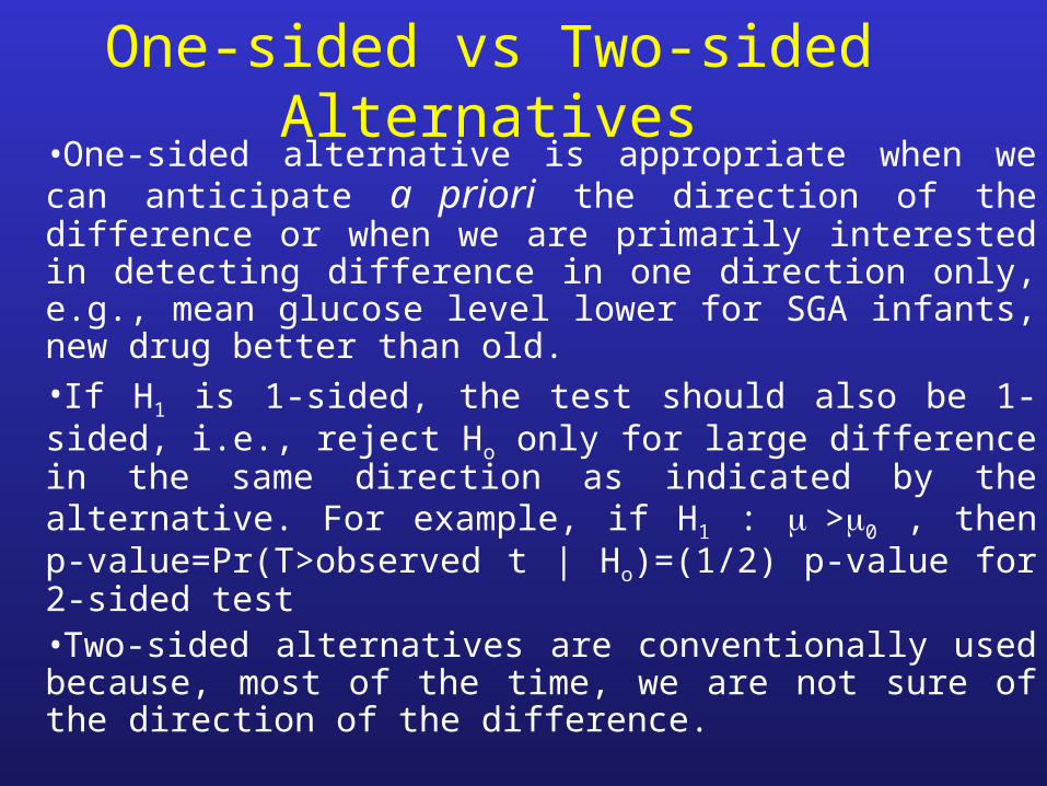
One-sided vs Two-sided Alternatives•One-sided alternative is appropriate when we can anticipate a priori the direction of the difference or when we are primarily interested in detecting difference in one direction only, e.g., mean glucose level lower for SGA infants, new drug better than old.•If H1 is 1-sided, the test should also be 1-sided, i.e., reject Ho only for large difference in the same direction as indicated by the alternative. For example, if H1 : >0 , then p-value=Pr(T>observed t | Ho)=(1/2) p-value for 2-sided test•Two-sided alternatives are conventionally used because, most of the time, we are not sure of the direction of the difference.

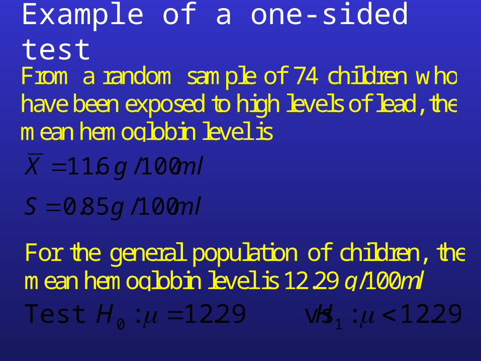
Example of a one-sided testFrom a random sample of 74 children whohave been exposed to high levels of lead, themean hemoglobin level is

mlgX 100/ 6.11

mlgS 100/ 85.0

29.12: vs29.12:Test 10 HH

For the general population of children, themean hemoglobin level is 12.29 g/100ml

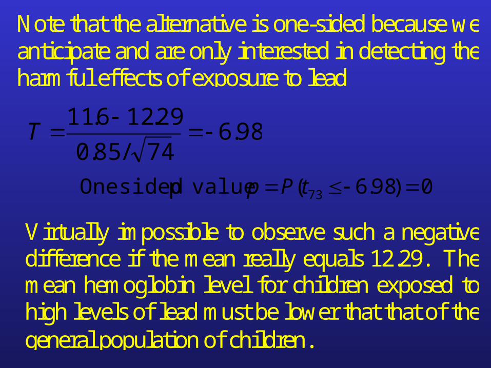
98.674/85.0

29.126.11

T

0)98.6( valuep sided One 73 tPp

Note that the alternative is one-sided because weanticipate and are only interested in detecting theharmful effects of exposure to lead

Virtually impossible to observe such a negativedifference if the mean really equals 12.29. Themean hemoglobin level for children exposed tohigh levels of lead must be lower that that of thegeneral population of children.

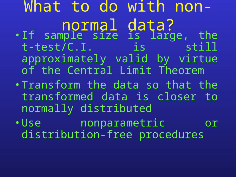
What to do with non-normal data?• If sample size is large, the t-test/C.I.

is still approximately valid by virtue of the Central Limit Theorem

• Transform the data so that the transformed data is closer to normally distributed

• Use nonparametric or distribution-free procedures

How large is large?• n >= 15 should suffice if the underlying

distribution is not too skewed and there are no outliers

• A smaller sample size may suffice if the data are closed to normally distributed

• n >= 40 should suffice even for fairly skewed populations