Hypothesis Testing

12/01/2011

Hypothesis-testing is a very important area of statistical inference.

It is a procedure which enables us to decide on the basis of information obtained from sample data whether to accept or reject a statement or an assumption about the value of a population parameter.

Such a statement or assumption which may or may not be true, is called a statistical hypothesis.

We accept the hypothesis as being true, when it is supported by the sample data.

We reject the hypothesis when the sample data fail to support it.

It is important to understand what we mean by the terms ‘reject’ and ‘accept’ in hypothesis-testing.

The rejection of a hypothesis is to declare it false.

The acceptance of a hypothesis is to conclude that there is insufficient evidence to reject it. Acceptance does not necessarily mean that the hypothesis is actually true.

The basic concepts

associated with hypothesis

testing are discussed below:

NULL AND ALTERNATIVE HYPOTHESES:

Null Hypothesis:

A null hypothesis, generally denoted by the symbol H0, is any hypothesis which is to be tested for possible rejection or nullification under the assumption that it is true.

A null hypothesis should always be precise such as

‘the given coin is unbiased’

or

‘a drug is ineffective in curing a particular disease’

or

‘there is no difference between the two teaching methods’.

The hypothesis is usually assigned a numerical value.

For example, suppose we think that the average height of students in all colleges is 62.

This statement is taken as a hypothesis and is written symbolically as H0 : = 62.

In other words, we hypothesize that = 62.

Alternative Hypothesis:

An alternative hypothesis is any other hypothesis which we are willing to accept when the null hypothesis H0 is

rejected. It is customarily denoted by H1 or

HA.

A null hypothesis H0 is thus tested against an alternative hypothesis H1.

For example, if our null hypothesis is H0 : = 62, then our alternative hypothesis may be H1 : 62 or H1 : < 62.

LEVEL OF SIGNIFICANCE

The probability of committing Type-I error can also be called the level of significance of a test.

Now, what do we mean by Type-I error?

In order to obtain an answer to this question, consider the fact that, as far as the actual reality is concerned, H0 is either actually true, or it is false.

Also, as far as our decision regarding H0 is concerned, there are two possibilities --- either we will accept H0, or we will reject H0.

The above facts lead to the following table:

Decision

Accept H0Reject H0

(or accept H1)

H0 istrue

Correct decision(No error)

Wrong decision(Type-I error)

TrueSituation

H0 isfalse

Wrong decision(Type-II error)

Correct decision(No error)

A close look at the four cells in the body of the above table reveals that the situations depicted by the top-left corner and the bottom right-hand corner are the ones where we are taking a correct decision.

On the other hand, the situation depicted by the top-right corner and the bottom left-hand corner are the ones where we are taking an incorrect decision.

The situation depicted by the top-right corner of the above table is called an error of the first kind or a Type I-error, while the situation depicted by the bottom left-hand corner is called an error of the second kind or a Type II-error.

In other words:

TYPE-I AND TYPE-II ERRORS:

On the basis of sample information, we may reject a null hypothesis H0, when it is, in fact, true or we may accept a null hypothesis H0, when it is actually false.

The probability of making a Type I error is conventionally denoted by and that of committing a Type II error is indicated by .

In symbols, we may write = P (Type I error)

= P (reject H0|H0 is true), = P (Type II error)

= P (accept H0|Ho is false).

TEST-STATISTIC

A statistic (i.e. a function of the sample data not containing any parameters), which provides a basis for testing a null hypothesis, is called a test-statistic.

Every test-statistic has a probability distribution (i.e. sampling distribution) which gives the probability that our test-statistic will assume a value greater than or equal to a specified value OR a value less than or equal to a specified value when the null hypothesis is true.

ACCEPTANCE AND REJECTION REGIONS

All possible values which a test-statistic may assume can be divided into two mutually exclusive groups:

one group consisting of values which appear to be consistent with the null hypothesis (i.e. values which appear to support the null hypothesis), and the other having values which lead to the rejection of the null hypothesis.

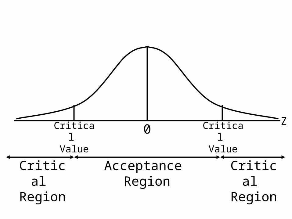
The first group is called the acceptance region and the second set of values is known as the rejection region for a test.

The rejection region is also called the critical region.

The value(s) that separates the critical region from the acceptance region, is called the critical value(s):

0Z

Acceptance Region

Critical Region

Critical Region

Critical Value

Critical Value

The critical value which can be in the same units as the parameter or in the standardized units, is to be decided by the experimenter.

The most frequently used values of , the significance level, are 0.05 and 0.01, i.e. 5 percent and 1 percent.

By = 5%, we mean that there are about 5 chances in 100 of incorrectly rejecting a true null hypothesis.

RELATIONSHIP BETWEEN THE LEVEL OF SIGNIFICANCE AND THE CRITICAL REGION:

The level of significance acts as a basis for determining the CRITICAL REGION of the test.

For example, if we are testing H0: = 45 against H1: 45, our test statistic is the standard normal variable Z, and the level of significance is 5%, then the critical values are Z = +1.96

Corresponding to a level of significance of 5%, we have:

0 1.96 Z-1.96

2.5%2.5%

Acceptance Region

Critical Region

Critical Region

ONE-TAILED AND TWO-TAILED TESTS:

A test for which the entire rejection region lies in only one of the two tails – either in the right tail or in the left tail – of the sampling distribution of the test-statistic, is called a one-tailed test or one-sided test.

A one-tailed test is used when the alternative hypothesis H1 is formulated in the following form:

H1 : > 0 or

H1 : < 0

For example, if we are interested in testing a hypothesis regarding the population mean, if n is large, and we are conducting a one-tailed test, then our alternative hypothesis will be stated as

H1 : > 0 or

H1 : < 0

In this case, the rejection region consists of either all z-values which are greater than + z or less than – z (where is the level of significance):

REJECT H0 if z < –z

0–zZREJECTION

REGION

If H0 : > 0

H1 : < 0

Then (in case of large n):

REJECT H0 if z > z/2

0 zZ

REJECTION REGION

If H0 : < 0

H1 : > 0

Then (in case of large n):

If, on the other hand, the rejection region is divided equally between the two tails of the sampling distribution of the test-statistic, the test is referred to as a two-tailed test or two-sided test.

In this case, the alternative hypothesis H1 is set up as:

H1 : 0

meaning thereby

H1 : < 0 or > 0

REJECT H0 if z < –z/2 or z > z/2

0–z/2

/2 /2

z/2REJECTION

REGIONREJECTION

REGION

If H0 : = 0

H1 : 0 Then (in case of large n):

EXAMPLE

A steel company manufactures and assembles desks and other office equipment at several plants in a particular country.

The weekly production of the desks of Model A at Plant-I has a mean of 200 and a standard deviation of 16.

Recently, due to market expansion, new production methods have been introduced and new employees hired.

The vice president of manufacturing would like to investigate whether there has been a change in the weekly production of the desks of Model A.

To put it another way, is the mean number of desks produced at Plant-I different from 200 at the 0.05 significance level?

The mean number of desks produced last year (50 weeks, because the plant was shut down 2 weeks for vacation) is 203.5.On the basis of the above result, should the vice president conclude that the there has been a change in the weekly production of the desks of Model A.

SOLUTION

We use the statistical hypothesis-testing procedure to investigate whether the production rate has changed from 200 per month.

Step-1:Formulation of the Null and

Alternative Hypotheses:

The null hypothesis is “The population mean is 200.”

The alternative hypothesis is ‘The mean is different from 200” or “The mean is not 200.”

These two hypotheses are written as follows:

H0 : = 200H1 : µ 200

Note:

This is a two-tailed test because the alternative hypothesis does not state a direction.

In other words, it does not state whether the mean production is greater than 200 or less than 200.

The vice president only wants to find out whether the production rate is different from 200.

Step-2:Decision Regarding the Level of

Significance (i.e. the Probability of Committing Type-I Error):

Here, the level of significance is 0.05.

This is , the probability of

committing a Type-I error (i.e. the risk of rejecting a true null hypothesis).

Step-3:Test Statistic (that statistic that will enable us to test our hypothesis):The test statistic for a large sample

mean is

Transforming the production data to standard units (z values) permits the use of the area table of the standard normal distribution.

n

Xz

Step-4: Calculations:

In this problem, we have n = 50, X = 203.5, and = 16.Hence, the computed value of z comes out to be:

55.15016

2005.203

n

Xz

Step-5:Critical Region (that portion of the X-axis which compels us to reject the

null hypothesis):

Since this is a two-tailed test, half of 0.05, or 0.025, is in each tail.

The area where H0 is not rejected, located between the two critical values, is therefore 0.95.

Applying the inverse use of the Area Table, we find that, corresponding to = 0.05, the critical values are 1.96 and -1.96, as shown below:

Decision Rule for the 0.05 Significance Level

Scale to z0-1.96-1.96 +1.96

H0 is not rejectedRegion of rejection

Region of rejection

Critical Value Critical Value

0.4750

0.4750

0.5000

025.02

05.0

2

025.0

2

05.0

2

0.5000

The decision rule is, therefore:

Reject the null hypothesis and accept the alternative hypothesis if the computed value of z is not between –1.96 and +1.96.

Do not reject the null hypothesis if z falls between –1.96 and + 1.96.

Step-6:Conclusion:

The computed value of z i.e. 1.55 lies between -1.96 and + 1.96, as shown below:

z scale0- 1.96 1.961.55

Computed value of z

Do not reject H0Reject H0 Reject H0

Because 1.55 lies between -1.96 and + 1.96, therefore, it does not fall in the rejection region, and hence H0 is not rejected.

In other words, we conclude that the population mean is not different from 200.

So, we would report to the vice president of manufacturing that the sample evidence does not show that the production rate at Plant-I has changed from 200 per week.

The difference of 3.5 units between the historical weekly production rate and the production rate of last year can reasonably be attributed to chance.

The above example pertained to a two-tailed test.

Let us now consider a few examples of one-tailed tests:

EXAMPLE

A random sample of 100 workers with children in day care show a mean day-care cost of Rs.2650 and a standard deviation of Rs.500.

Verify the department’s claim that the mean exceeds Rs.2500 at the 0.05 level with this information.

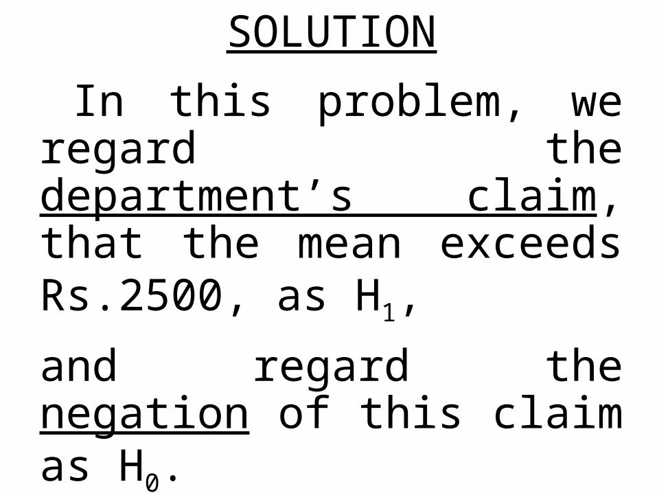
SOLUTION

In this problem, we regard the department’s claim, that the mean exceeds Rs.2500, as H1,

and regard the negation of this claim as H0.

Thus, we have

i) H0 : < 2500H1 : > 2500 (exceeds 2500)

(Important Note: We should always regard that hypothesis as the null hypothesis which contains the equal sign.)

ii) We are given the significance level at = 0.05.

iii) The test-statistic, under H0 is

which is approximately normal as n = 100 is large enough to make use of the central limit theorem.

,nS

XZ 0

0 Z0.05

=1.645

ZREJECTION

REGION

0.05

iv) The rejection region is Z > Z0.05 = 1.645

v) Computing the value of Z from sample information, we find

350

150

100500

25002650z

vi) Conclusion:

Since the calculated value z = 3 is greater than 1.645, hence it falls in the rejection region, and, therefore, we reject H0, and may conclude that the department’s claim is supported by the sample evidence.

An Interesting and Important Point:

For = 0.01, Z = 2.33.

As our computed value of Z i.e. 3 is even greater than 2.33, the computed value of X is highly significant.

(With only 1% chance of being wrong, the department’s claim was correct).

EXAMPLE

A survey conducted by a market-research organization five years ago showed that the estimated hourly wage for temporary computer analysts was essentially the same as the hourly wage for registered nurses.

This year, a random sample of 32 temporary computer analysts from across the country is taken.

The analysts are contacted by telephone and asked what rates they are currently able to obtain in the market-place.

A similar random sample of 34 registered nurses is taken.

The resulting wage figures are listed in the following table:

Computer Analysts Registered Nurses

$ 24.10 $25.00 $24.25 $20.75 $23.30 $22.7523.75 22.70 21.75 23.80 24.00 23.0024.25 21.30 22.00 22.00 21.75 21.2522.00 22.55 18.00 21.85 21.50 20.0023.50 23.25 23.50 24.16 20.40 21.7522.80 22.10 22.70 21.10 23.25 20.5024.00 24.25 21.50 23.75 19.50 22.6023.85 23.50 23.80 22.50 21.75 21.7024.20 22.75 25.60 25.00 20.80 20.7522.90 23.80 24.10 22.70 20.25 22.5023.20 23.25 22.4523.55 21.90 19.10

Conduct a hypothesis test at the 2% level of significance to determine whether the hourly wages of the computer analysts are still the same as those of registered nurses.

SOLUTIONHypothesis Testing Procedure:

Step-1:Formulation of the Null and Alternative

Hypotheses:

H0 : 1 – 2 = 0 HA : 1 – 2 0(Two-tailed test)

Step-2:Level of Significance: = 0.02

Step-3:Test Statistic:

2

22

1

21

2121

nn

XXZ

Step-4:Calculations:The sample size, sample

mean and sample standard deviation for each of the two samples are given below:

Computer Analysts: n1 = 32

X 1 = $23.14 S1

2= 1.854

Registered Nurses: n2 = 34

X2 = $21.99 S2

2= 1.845

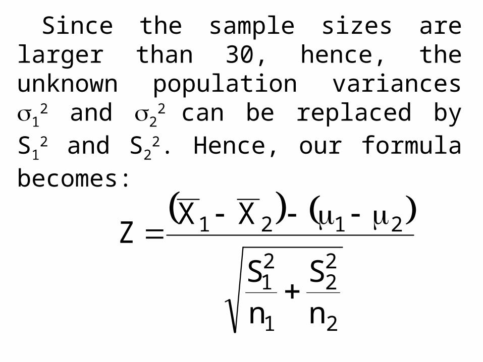
Since the sample sizes are larger than 30, hence, the unknown population variances 1

2 and 22 can be replaced by S1

2 and S2

2. Hence, our formula becomes:

2

22

1

21

2121

nS

nS

XXZ

Hence, the computed value of Z comes out to be :

43.3

335.0

15.1

34845.1

32854.1

099.2114.23Z

Step-5:Critical Region:As the level of

significance is 2%, and this is a two-tailed test, hence, we have the following situation:

0Z.01 = -2.33 Z.01 = +2.33

/2 = .01 /2 = .010.490.49

Hence, the critical region is given by

| Z | > 2.33

Step-6:Conclusion:

As the computed value i.e. 3.43 is greater than the tabulated value 2.33, hence, we reject H0.

Z = 0Z.01 = -2.33 Z.01 = +2.33Z

Calculated Z = 3.43

21 XX 15.1XX 21 021

The researcher can say that there is a significant difference between the average hourly wage of a temporary computer analyst and the average hourly wage of a temporary registered nurse.

The researcher then examines the sample means and uses common sense to conclude that, on the average, temporary computer analyst earn more than temporary registered nurses.

Let us consolidate the above concept by considering another example:

EXAMPLE

Suppose that the workers of factory B believe that the average income of the workers of factory A exceeds their average income.

A random sample of workers is drawn from each of the two factories, an the two samples yield the following information:

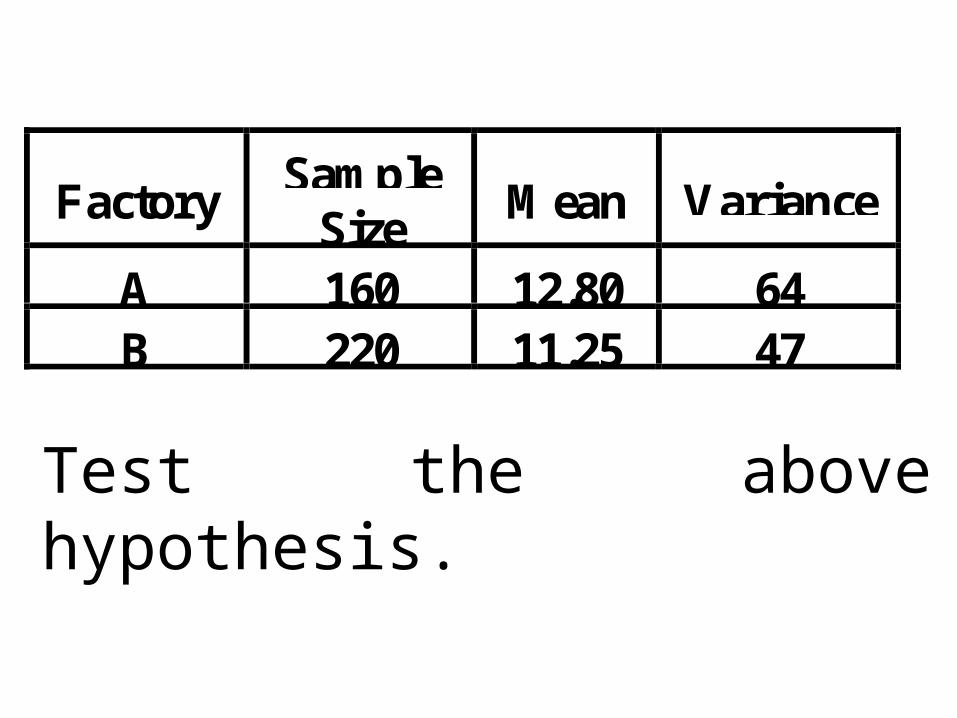
FactorySample

SizeMean Variance

A 160 12.80 64B 220 11.25 47

Test the above hypothesis.

SOLUTION

Let subscript 1 denote values pertaining to Factory A, and let subscript 2 denote values pertaining to Factory B.

Then, we proceed as follows:

Hypothesis-testing Procedure:

Step 1: H0 : 1 < 2 (or 1 - 2 < 0)HA : 1 > 2 (or 1 - 2 > 0).

Step 2:

Level of significance = 5%.

Steps 3 & 4:

22047

16064

25.1180.12

ns

ns

0xxZ

2

22

1

21

21

99.178.0

55.1

61.0

55.1

Step 5:Critical Region:Since it is a right-tailed test, hence the critical region is given by

Z > Z0.05

i.e. Z > 1.645

Step 6: Conclusion:

Since 1.99 is greater than 1.645, hence H0 should be rejected in favour of HA.

The sample evidence has consolidated the belief of the workers of factory B.

Next, we consider the case when we are interested in conducting a test regarding p, the proportion of successes in the population.

We illustrate this situation with the help of the following example:

EXAMPLE

A sociologist has a hunch that not more than 50% of the children who appear in a particular juvenile court three times or more are orphans.

To test this hypothesis, a sample of 634 such children is taken and it is found that 341 of these children are orphans, (one or both parents dead).

Test the above hypothesis using 1% level of significance.

SOLUTION

Hypothesis-testing Procedure:

Step 1:H0 : p < 0.50HA : p > 0.50 (one-tailed test)

Step 2:Level of significance: = 1%

00

021

p1pn

pnXZ

Step 3: Test statistic:

(where + ½ denotes the continuity correction)

Step 4: Computation:

Here np0 = 634 (0.50) = 317and X = 341Hence X > np0 so use X - ½

S o 59.12

5.23

50.050.0634

317341Z 2

1

= 1 . 8 7

Step 5: Critical region:

Since = 0.01, hence the critical region is given by

Z > 2.33

Step 6: Conclusion:

Since 1.87 < 2.33,hence the computed Z does not fall in the critical region.

Hence, we conclude that the sociologist’s hunch is acceptable.