hypothesis esting: person-time data chapter 14.pdf · section 14.1 measures of effect for...

226

HYPOTHESIS TESTING:PERSON-TIME

DATA

REVIEW OF KEY CONCEPTS .........................................................................................................................................................................................

SECTION 14.1 Measures of Effect for Person-Time Data .........................................................................................................................................................................................

1. Incidence Density ( λ ) Number of events/amount of person-time. It represents the number of disease

events per unit time. In subsequent discussion, we will use the term incidence rate synonymously with incidence density.

2. Cumulative Incidence CI t( ) The probability of developing a disease over a time period t( ) . The relationship between cumulative incidence and incidence density is

CI t t t( ) = − − ≅1 exp λ λa f , for small λ t

Approximately 100,000 women in the Nurses’ Health Study, ages 30–64, were followed for 1,140,172 person-years from 1976 to 1990, during which time 2214 new breast cancers occurred. The incidence density for breast cancer was 2214 1140 172 000194, , .= events per person-year or 194 events per 100,000 (105 ) person-years. The cumulative incidence of breast cancer over 5 years is

1 5 0 00194 0 00966 966− − = =( )exp . . events per 105 person-years. .........................................................................................................................................................................................

SECTION 14.2 One Sample Inference for Incidence Rate Data .........................................................................................................................................................................................

Suppose an investigator wants to test the hypothesis that exposure to hair dyes increases the risk of breast cancer. She collects data from 1000 postmenopausal women age 50–59 without previous cancer who have been employed as beauticians for at least 10 years and follows each of them for a 6 year period. She finds that 20 of them have developed breast cancer over this period. The expected incidence rate of breast cancer is 200 events per 105 person-years for women in this age group. Does the risk of breast cancer seem elevated in this occupational group? To address this question, we test the hypothesis H0 : µ µ= 0 vs H1 : µ µ≠ 0 , where

STUDY GUIDE/FUNDAMENTALS OF BIOSTATISTICS 227

0

the expected number of events among beauticiansthe expected number of events if beauticians have the same incidence rate as thegeneral population

µµ

==

We use the test statistic

X X2 02

012=

− µµ

χa f ~ under H0 ,

where

X = observed number of events among beauticians. The p-value is given by Pr χ1

2 2> Xb g . In this case, we have 6000 person-years. Thus, µ0

56000 200 10 12= =b g . Therefore, the test statistic is

X22

1220 12

125 33=

−=

( ). ~ χ under H0

Because χ χ1 975

2 21 9925 02 6 63, . , .. .= < < =X , it follows that . .01 025< <p . Thus, there is a significant

excess risk of breast cancer among beauticians. The above procedure is a large sample procedure which is only valid if µ0 10> . The corresponding small sample procedure is based on exact Poisson probabilities and is given in Equation 14.5, Chapter 14, text. 14.2.1 Point and Interval Estimation of Incidence Rates A point estimate of the incidence rate is given by x T , where x = number of events and T = amount of person-time. In the breast cancer example, we have x = 20 and T = 6000 person-years. Therefore, the estimated incidence rate = =20 6000 333 events per 105 person-years. To obtain a 100% × −( )1 α CI for the underlying incidence rate, we first compute a confidence interval for the expected number of events ( µ ) given by c c1 2,a f , which is obtained from

x z x± −1 2α if x ≥ 10

or the x row and 1−α column of Table 8, text if x < 10 . The corresponding 100% × −( )1 α CI for the incidence rate = c T c T1 2,a f . In this example, x = 20 . Thus, the 95% CI for µ is

20 196 20 20 88 112, 288± = ± =. . . .a f The corresponding 95% CI for the incidence rate is

1126000

2886000

18710

479105 5

. , . ,FH

IK =FH

IK

228 CHAPTER 14/HYPOTHESIS TESTING: PERSON-TIME DATA

.........................................................................................................................................................................................

SECTION 14.3 Comparison of Incidence Rates .........................................................................................................................................................................................

Women were asked whether their mothers or any sisters had ever had breast cancer. If they responded yes, then they were considered to have a family history of breast cancer. From 1976 to 1990, there were 295 cases of breast cancer over 80,539 person-years among women with a family history of breast cancer and 1919 cases over 1,059,633 person-years among women without a family history. How can we compare the two incidence rates? We wish to test the hypothesis H0 : ID ID1 2= versus H1 : ID ID1 2≠ (where ID = incidence density). We use the test statistic

z a EV

N=− −

( )1 1

1

5 0 1. ~ , under H0

where

a i it i i

E H a a tt t

V H a a t tt t

i

i

= =

= =

= = =++

= =++

observed number of cases in group ,number of person - years in group ,

expected number of cases in group 1 (family history yes) under

variance of number of cases in group 1 under

1 21 2

1 01 2 1

1 2

1 01 2 1 2

1 22

,,

a f

a fa f

The p-value = × ( )2 Φ z if z < 0 , or = × − ( )2 1 Φ z if z ≥ 0 . This test should only be used if V1 5≥ . In this case, we have a1 295= , a2 1919= , t1 80 539= , , t2 1059,633= , . Therefore, 1 2 2214a a+ = , t t1 2 1140 172+ = , , and

E

V

1

1 2

2214 80 5391140172

1564

2214 80 539 1059,6331140 172

1453

= FHG

IKJ =

=( )( )( )

=

,, ,

.

, ,, ,

.

The test statistic is

z N H=− −

= = ( )295 156 4 5

145 31381121

1146 0 1 0. ..

..

. ~ , under

The p-value = × − <( )2 1 11 46 001Φ . . . Thus, women with a family history have a significantly higher incidence rate of breast cancer than women without a family history. If V1 5< , then exact methods based on the binomial distribution must be used [see Equation 14.9, Chapter 14, text].

.........................................................................................................................................................................................

SECTION 14.4 Estimation of the Rate Ratio .........................................................................................................................................................................................

The rate ratio (RR) is defined by

RR = incidence rate in an exposed group/incidence rate in an unexposed group It is estimated by a t a t RR1 1 2 2a f a f = .


To obtain confidence limits for RR, we first obtain confidence limits for ln ,RR c c( ) = 1 2a f given by

c RR za a

c RR za a

1 1 21 2

2 1 21 2

1 1

1 1

= − +

= + +

−

−

ln

ln

d i

d i

α

α

The corresponding 100% × −( )1 α CI for RR c c= exp , exp1 2a f a f . The estimated incidence rate for women with a family history = =295 80 539 366 105, , and for women without a family history = =1919 1059,633 181 105, . The estimated RR for women with a family history of breast cancer versus women without a family history = =366 10 181 10 2 025 5b g b g . . A 95% CI for RR is given by exp , expc c1 2a f a f , where

c

c

1

2

2 02 196 1295

11919

0704 0123 0582

0704 0123 0827

= ( ) − + = − =

= + =

ln . . . . .

. . .

Thus, the 95% CI for RR = ( ) ( ) =exp . , exp . . .0582 0827 179, 2 29a f .

.........................................................................................................................................................................................

SECTION 14.5 Inference for Stratified Person-Time Data .........................................................................................................................................................................................

In the breast-cancer data, it is possible that women who report a family history (Hx) of breast cancer are older than those women who do not report such a history, since their mothers and sisters are likely to be older. Since breast-cancer incidence rises with age, it is important to control for age in the analysis. To accomplish this, we obtain age-specific incidence rates of breast cancer for women with and without a family history as shown here:

Family Hx = yes Family Hx = no Age

Cases

Person- years

Incidence rate (× −10 5 )

Cases

Person- years

Incidence rate (× −10 5 )

30-39 12 8,564 140 124 173,104 72 40 44 31 12,157 255 268 200,916 133 45-49 54 15,422 350 387 215,329 180 50-54 68 18,110 375 461 214,921 214 55-59 86 16,384 525 416 165,380 252 60-64 44 9,902 444 263 89,983 292 Total 295 80,539 366 1,919 1,059,633 181

We wish to test the hypothesis H0 : RR = 1 versus H1 : RR ≠ 1 , where RR = rate ratio for women with a family history versus women without a family history within a specific age group. We use the test statistic

X A E AA

22

125

=− −( )( )

( )

. ~Var

χ under H0

where


a t ii k

a t ii k

A a

E A a a tt t

A a

i i

i i

ii

k

i i i

i ii

k

i

1 1

2 2

11

1 2 1

1 21

1

1

1

,, ,

,, ,

=

==

=

= =

= =++

= =+

=

=

∑

∑( )

( )

number of casesand person-years for women with a family history in the th age group,

number of casesand person-years for women without a family history in the th age group,

total observed number of cases among women with a family history over all strata

total expected number of cases among women with a family history over all strata

Var variance of total number of cases among women with a family history over all strata

…

…

a f

a t tt t

i i i

i ii

k2 1 2

1 22

1

a fa f+=

∑

The p-value = >Pr χ1

2 2Xb g . We should only use this test if Var A( ) ≥ 5. In this case,

A

E A

A

X

p

=

=++

+ ++

+= + + =

=+

++ +

++

= + + =

=− −( )

= =

= > <

( )( )( )

( )

( )( )

( )

( )( )( )( )

( )

( )( )( )

( )

29512 124 85648564 173104

44 263 99029902 89 983

6 41 30 43 169 7412 124 8564 173104

8564 17310444 263 9902 89 983

9902 89 983611 27 42 156 20

295 169 74 5156 20

124 76156 20

99 65

99 65 001

2 2

22 2

12

, ,. . .

,,

,,

. . .

. ..

..

.

. .

…

…

…

…

Var

- value Pr χa f Therefore, women with a family history of breast cancer have significantly higher breast-cancer incidence rates than women without a family history, even after controlling for age. 14.5.1 Estimation of the Rate Ratio for Stratified Data To estimate the rate ratio for stratified data, we compute a weighted average of the log rate ratios within specific strata and then take the antilog of the weighted average. This estimate is referred to as an adjusted rate ratio. Specifically, RR = estimated adjusted rate ratio = ( )exp c , where

cw RR

w

i ii

k

ii

k= =

=

∑

∑

lnd i1

1

and

RR at

at

i

wa a

ii

i

i

i

ii i

= FHGIKJFHGIKJ =

= +FHG

IKJ−

1

1

2

2

1 2

11 1

estimated rate ratio in the th stratum

A 100% × −( )1 α CI for RR is given by exp , expc c1 2a f a f , where


1 1 2 2 1 2

1 1

1 1,k k

i ii i

c c z c c zw w

α α− −

= =

= − = +

∑ ∑

For the breast-cancer data, we have

RR

w

1

1401072

10

1

1

5

5

196

112

1124

10 94

= =

= +FH IK =−

.

. etc.

The RR’s and wi ’s for each of the age groups are given as follows:

Age group RRi wi

30–39 1.96 10.94 40–44 1.91 27.79 45–49 1.95 47.39 50–54 1.75 59.26 55–59 2.09 71.27 60–64 1.52 37.69

Therefore,

c

RR

c

c

=+ ++ +

= =

= =

= − = − =

= + =

( ) ( )

( )

10 94 196 37 69 15210 94 37 69

158 35254 33

0 623

0 623 186

0 623 196 1254 33

0 623 0123 0 500

0 623 0123 0 745

1

2

. ln . . ln .. .

.

..

exp . .

. ..

. . .

. . .

……

The 95% CI for the age-adjusted RR is given by exp . , exp . . , .0500 0745 165 211( ) ( ) = a f . Notice that the age-adjusted rate ratio is slightly lower than the crude rate ratio of 2.02 computed in Section 14.4, indicating that women with a family history are somewhat older than women without a family history. Therefore, the age-adjusted rate ratio is more appropriate in this case. We have assumed in the breast-cancer analyses that the underlying rate ratio is the same in all age groups. To check this assumption, a test for the homogeneity of the rate ratios over different strata can be performed [see Equation 14.32, Chapter 14, text]. Sample size estimation for stratified (e.g., by age) incidence rate data depends on (1) the age-specific incidence rates of disease in the unexposed group, (2) the distribution of person-years within age-exposure-specific groups, (3) the true rate ratio under H1 , and (4) type I and type II errors. The appropriate formula is given in Equation 14.33, Chapter 14, text. Similarly, estimation of power for stratified incidence rate data with a specified sample size is given in Equation 14.34, Chapter 14, text.

.........................................................................................................................................................................................

SECTION 14.6 Testing for Trend-Incidence Rate Data .........................................................................................................................................................................................

It appears from Section 14.5 that the incidence rate of breast cancer increases with age. However, the rate of increase is greater prior to age 45 than after age 45. Suppose we wish to estimate the rate of increase after age 45 and wish to control for the confounding effect of family history. We assume a model of the form


ln p Sij i jc h = +α β

where

p i j i s j k

S jij

j

= = =

=

incidence rate for the th family history (Hx) group and th age group,

score variable for the th age group

1 1, , , , ,… …

Thus, within a family history group, log incidence is assumed to be a linear function of the score vari-able S j with slope = β . We estimate β within the ith family Hx group by

,

,

ˆ xy ii

xx i

LL

β =

where

( )( )

1 1,

1

1

2

12,

1

1

ˆlnˆln

number of breast cancer cases for the th family Hx group and th age group.

k k

ij j ij ijkj j

xy i ij j ij kj

ijj

k

ij jkj

xx i ij j kj

ijj

ij ij

w S w pL w S p

w

w SL w S

w

w a i j

= =

=

=

=

=

=

= −

= −

= =

∑ ∑∑

∑

∑∑

∑

Then ( ) ( )1 2,

ˆ 1i xx ise Lβ = , with test statistic ( ) ( )ˆ ˆ 0,1i i iz se Nβ β= ∼ under H0, with

( )[ ]-value 2 1 ip z= × −Φ . To obtain an overall estimate of the slope, we compute

, ,1 1

ˆs s

xy i xx ii i

L Lβ= =

= ∑ ∑

with standard error given by ( ) ,1

ˆ 1s

xx ii

Lse β=

= ∑ . The corresponding test statistic is

( ) ( )ˆ ˆ 0,1z se Nβ β= ∼ under H0. The two-sided ( )[ ]-value 2 1p z= × −Φ .

We will assume that S j = 1 for age 45–49, 2 for age 50–54, 3 for age 55–59 and 4 for 60–64. In this case,

i = 1 corresponds to family Hx = yes and i = 2 to family Hx = no. The estimated slope within each family Hx group and overall is given in the following spreadsheet:


Family Hx = yes

Age Score ( )ijS wij person-

years incidence ij ijw S 2ij ijw S xxL ( )lnijw pij ( )lnijw S pij ij Lxy Beta se z p-value

45-49 1 54 15422 0.00350 54 54 -305.3466 -305.35 50-54 2 68 18110 0.00375 136 272 -379.7604 -759.52 55-59 3 86 16384 0.00525 258 774 -451.4753 -1354.43 60-64 4 44 9902 0.00444 176 704 -238.3173 -953.27

252 624 1804 258.86 -1374.9 -3372.56 31.95 0.123 0.062 1.986 .047

Family Hx = no

Age Score ( )ijS wij person-

years incidence ij ijw S 2ij ijw S xxL ( )lnijw pij ( )lnij ijw S pij Lxy Beta se z p-value

45-49 1 387 215329 0.00180 387 387 -2446.42 -2446.42 50-54 2 461 214921 0.00214 922 1844 -2832.673 -5665.35 55-59 3 416 165380 0.00252 1248 3744 -2489.891 -7469.67 60-64 4 263 89983 0.00292 1052 4208 -1534.663 -6138.65

1527 3609 10183 1653.28 -9303.648 -21720.09 268.68 0.163 0.025 6.608 < .001

Overall 1779 1912.14 300.64 0.157 0.023 6.875 < .001 Therefore, the overall estimate of the slope is

300.64ˆ 0.1571912.14

β = =

Thus, breast-cancer incidence increases by 0.157 17%e = per 5-year increase in age, or roughly

0.157 5 3.2%e = per year after age 45. To obtain a standard error for the slope, we use

( ) 1 1ˆ 0.0231912.14xx

seL

β = = =

Therefore, a 95% CI for β is ( ) ( )0.157 1.96 0.023 0.157 0.045 0.112, 0.202± = ± = . The corresponding 95% CI for the rate of increase is ( ) ( )[ ] ( )exp 0.112 , exp 0.202 11.8%, 22.4%= per 5-year increase in age or (2.3%, 4.1%) per year after age 45. If we wish to test the hypothesis H0 : β = 0 versus H1 : β ≠ 0 , we can use the test statistic

( ) ( )ˆ 0.157 6.88 ~ 0, 1ˆ 0.023

z Nseββ

= = = under H0

The p-value = × ( )2 Φ z if z < 0 or = × − ( )2 1 Φ z if z ≥ 0 . In this case, ( )[ ]2 1 6.88 .001p = × −Φ < . Thus, breast-cancer incidence significantly increases with age after age 45.

.........................................................................................................................................................................................

SECTION 14.7 Introduction to Survival Analysis .........................................................................................................................................................................................

For incidence rates that remain constant over time, the methods in Sections 14.1–14.6 are applicable. If incidence rates vary over time, then methods of survival analysis are more appropriate. In the latter case, the hazard function plays a similar role to that of incidence density except that it is allowed to vary over time.


The hazard function h t( ) is the instantaneous probability of having an event at time t (per unit time) given that one has not had an event up to time t. A group of 1676 children were followed from birth to the 1st year of life for the development of otitis media (OTM), a common ear condition characterized by fluid in the middle ear (either the right or the left ear) and some clinical symptoms (e.g., fever, irritability). The presence of OTM was determined at every clinic visit. For simplicity the data are reported here in 3-month intervals (i.e., it is assumed that the episodes of OTM occur exactly at 3 months, 6 months, 9 months, and 12 months).

Time (t) Fail Censored Survive Total h t( ) S t( ) 3 121 32 1523 1676 0.0722 .9278 6 250 53 1220 1523 0.1641 .7755 9 283 41 896 1220 0.2320 .5956 12 182 714 0 896 0.2031 .4746

The hazard at 3 months = the number of children who failed (i.e., had an episode of OTM) at 3 months divided by the number of children available for examination at 3 months 121 1676 0.0722= = . Similarly, the hazards at 6, 9, and 12 months are 0.1641, 0.2320, and 0.2031, respectively, where the denominators at 6, 9, and 12 months are the number of children available for examination at these times who had not had an episode prior to these times. Clearly, the hazard function appears to vary over time. 14.7.1 Censored Data In a clinical study, some patients have not failed up to a specific point in time. If these patients are not followed any longer, they are referred to as censored observations. For example, in the OTM study, 32 children were censored at 3 months; these children were followed for 3 months, did not develop OTM at that time, and were not followed any further. An additional 1523 children also did not fail at 3 months but were followed further and are listed as surviving. The two groups are distinguished because they are treated differently in the estimation of survival curves.

.........................................................................................................................................................................................

SECTION 14.8 Estimation of Survival Curves .........................................................................................................................................................................................

Suppose there are Si−1 subjects who survive up to time ti−1 and are not censored at that time. Of these sub-jects, Si survive, di fail, and li are censored at time ti . The Kaplan-Meier estimator of survival at time ti is

S t dS

dS

dSi

i

ia f = −FHGIKJ × −FHGIKJ × −FHG

IKJ−1 1 11

0

2

1 1…

For the OTM data, the estimated survival probability at 3 months = −( ) =1 121 1676 9278. . The estimated survival probability at 6 months = −( ) × −( ) =1 121 1676 1 250 1523 7755. , …, etc. It is estimated that 47% of children “survive” (i.e., do not have OTM for 1 year). Thus, 53% of children have a 1st episode of OTM during the 1st year of life.

.........................................................................................................................................................................................

SECTION 14.9 Comparison of Survival Curves .........................................................................................................................................................................................

It is interesting to compare survival curves between different subgroups. For example, one hypothesis is that infants of smoking mothers have more OTM than infants of nonsmoking mothers. How can we test this hypothesis? We have computed separate survival curves for infants of smoking and nonsmoking mothers as follows:


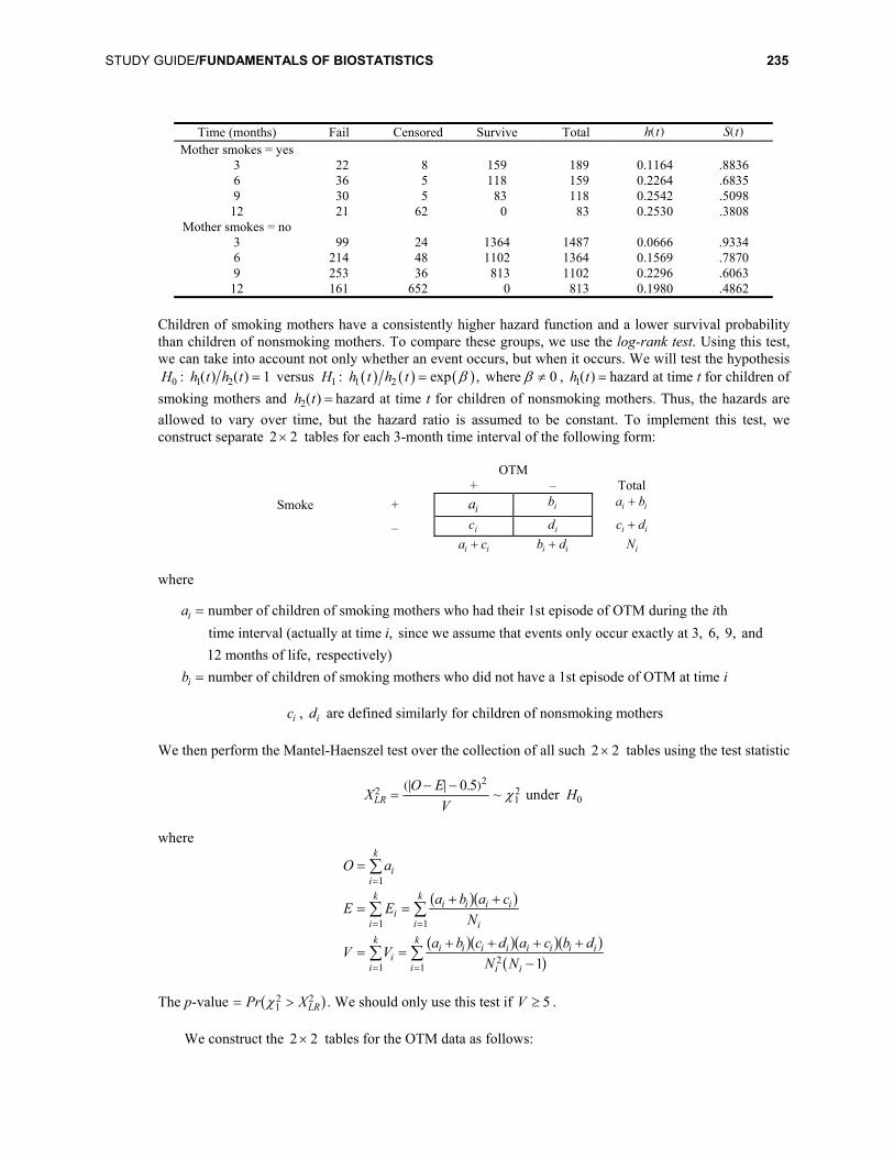
Time (months) Fail Censored Survive Total h t( ) S t( )

Mother smokes = yes 3 22 8 159 189 0.1164 .8836 6 36 5 118 159 0.2264 .6835 9 30 5 83 118 0.2542 .5098

12 21 62 0 83 0.2530 .3808 Mother smokes = no

3 99 24 1364 1487 0.0666 .9334 6 214 48 1102 1364 0.1569 .7870 9 253 36 813 1102 0.2296 .6063

12 161 652 0 813 0.1980 .4862 Children of smoking mothers have a consistently higher hazard function and a lower survival probability than children of nonsmoking mothers. To compare these groups, we use the log-rank test. Using this test, we can take into account not only whether an event occurs, but when it occurs. We will test the hypothesis H0 : h t h t1 2 1( ) ( ) = versus H1 : ( ) ( ) ( )1 2 exp , where 0h t h t β β= ≠ , h t1( ) = hazard at time t for children of smoking mothers and h t2( ) = hazard at time t for children of nonsmoking mothers. Thus, the hazards are allowed to vary over time, but the hazard ratio is assumed to be constant. To implement this test, we construct separate 2 2× tables for each 3-month time interval of the following form:

OTM + – Total Smoke + ai bi a bi i+

– ci di c di i+ a ci i+ b di i+ Ni

where

a ii

b i

i

i

=

=

number of children of smoking mothers who had their 1st episode of OTM during the th time interval (actually at time , since we assume that events only occur exactly at 3, 6, 9, and 12 months of life, respectively)number of children of smoking mothers who did not have a 1st episode of OTM at time

ci , di are defined similarly for children of nonsmoking mothers

We then perform the Mantel-Haenszel test over the collection of all such 2 2× tables using the test statistic

X O EVLR

2 =− −( )0 5 2

12. ~ χ under H0

where

O a

E E a b a cN

V V a b c d a c b dN N

ii

k

ii

ki i i i

ii

k

ii

ki i i i i i i i

i ii

k

=

= =+ +

= =+ + + +

−

=

= =

= =

∑

∑ ∑

∑ ∑

1

1 1

12

1 1

a fa f

a fa fa fa fa f

The p-value = >Pr χ1

2 XLR2a f . We should only use this test if V ≥ 5 .

We construct the 2 2× tables for the OTM data as follows:


3 months OTM + – Total Smoke + 22 167 189 – 99 1388 1487 Total 121 1555 1676

6 months

OTM + – Total Smoke + 36 123 159 – 214 1150 1364 Total 250 1273 1523

9 months


12 months


Thus,

O

E

V

= + + =

=( )

+ +( )

= + + =

=( )( )( )

( )+ +

( )( )( )( )

= + + =

22 21 109189 121

167683 182

8961364 1686 8398

121 1555 189 14871676 1675

182 714 83 813896 895

1124 12 20 62 002 2

…

… …

… …

. . .

. . .

The test statistic is

XLR2

2

12109 83 98 5

62 006014162 00

9 70=− −( )

= =. ..

..

. ~ χ under H0

The p-value = > =Pr χ1

2 9 70 002. .a f . Thus, children of smoking mothers have significantly more first episodes of OTM during the 1st year of life than children of nonsmoking mothers.

.........................................................................................................................................................................................

SECTION 14.10 The Proportional-Hazards Model .........................................................................................................................................................................................

The log-rank test is useful for comparing survival curves between two groups. It can be extended to allow one to control for a limited number of other covariates as well. However, if there are many covariates to be controlled for, then using a proportional-hazards model is preferable. The Cox proportional-hazards model is a regression-type approach for modeling survival data. If we have k variables of interest, x xk1, ,… , then the hazard at time t is modeled as

h t h t x xk k( ) = ( ) + +0 1 1exp β β…a f


where

h t0( ) = hazard function at time t for a subject with all covariate values = 0 14.10.1 Interpretation of Parameters 1. Dichotomous predictors If xi is a dichotomous predictor of OTM (e.g., sex, where 1 = female and

0 = male), then exp β ia f = ratio of hazards for OTM for females versus males, all other factors held constant.

2. Continuous predictors If xi is a continuous predictor variable [e.g., weight (lbs)], then exp β ia f = hazard ratio for OTM for the heavier versus the lighter of two infants that are 1 lb apart in weight, all other variables held constant.

14.10.2 Hypothesis Testing To test the hypothesis H0 : β i = 0 , all other β j ≠ 0 , versus H1 : all β j ≠ 0 , we use the test statistic

zse

Ni

i

= ( )~ ,ββe j

0 1 under H0 .

The p-value = × ( )2 Φ z if z < 0 , or = × − ( )2 1 Φ z if z ≥ 0 . We have run the Cox proportional-hazards model with the OTM data, where the risk factors are 1. Sex (coded as 1 if female and 0 if male) 2. At least one sibling with Hx (history) of ear disease (coded as 1 if yes and 0 if no) 3. Some sibs, but none with a Hx of ear disease (coded as 1 if yes and 0 if no) 4. Ever breastfed during the 1st year of life (coded as 1 if yes and 0 if no) 5. Mother smoking (ever during the 1st year of life) (coded as 1 if yes and 0 if no) The results are as follows:

Variable Regression coefficient Standard error z p–value Relative riskSex –0.080 0.069 –1.16 .25 0.92 Sibs with Hx ear disease 0.331 0.073 4.53 < .001 1.39 Sibs, no Hx ear disease 0.207 0.120 1.73 .085 1.23 Ever breastfed 0.047 0.075 0.63 .53 1.05 Mother smoking 0.223 0.106 2.10 .035 1.25

There are significant effects of maternal smoking, even after controlling for the other covariates ( p = .035). The relative risk = hazard ratio = 125. ; thus, children whose mothers smoke are 25% more likely to develop a 1st episode of OTM at any point in time in the 1st year of life given that they haven’t developed OTM previously compared with children whose mothers do not smoke, all other risk factors being equal. In addition, there was a significant effect of having a sibling with a Hx of ear disease versus not having any sibs ( RR = 139. , p < .001). The other covariates were not statistically significant. In addition, it is possible to obtain confidence limits for both the true regression coefficients and RR’s. Specifically, a 95% CI for the regression coefficient for maternal smoking is

0 223 196 0106 0 015 0 431. . . . , .± = ( )( ) . The corresponding 95% CI for RR is exp . , exp . . .0015 0431 102, 154( ) ( ) = a f .


Finally, it is possible to calculate power for the comparison of 2 survival curves under a proportional hazards model as a function of the relative risk and the total expected number of events (see Equation 14.47, Chapter 14, text).

PROBLEMS ..................................................................................................................... Cancer Refer to the data in Table 14.4 (text, Chapter 14). 14.1 Obtain an estimate of the rate ratio of breast cancer for

past postmenopausal hormone users vs. never users, and provide a 95% CI about this estimate (control for age in your analysis).

14.2 Test the hypothesis that past use of postmenopausal

hormones is associated with an increased (or decreased) risk of breast cancer compared with never users (control for age in your analysis).

14.3 Suppose we plan a new study and assume that the true

rate ratio comparing breast-cancer incidence of past to never users is 1.2. How many subjects do we need to study if (a) each subject is followed for 10 years, (b) the distribution of person-years among past and never users is the same as in Table 14.4 (Chapter 14, text), (c) the age-specific incidence rate of breast cancer among never users is the same as in Table 14.4, and (d) we wish to conduct a two-sided test with α = .05 and power = 80% ?

14.4 Suppose that the planners of the study expect to enroll 10,000 postmenopausal women who are past or never PMH users and follow each of them for 10 years. How much power would such a study have under the assumptions given in Problem 14.3?

Cardiovascular Disease A proportional-hazards model was obtained using SAS PROC PHGLM based on the Framingham Heart Study data presented in Example 13.36 (Chapter 13, text). The exam when the 1st event occurred for an individual was used as the time of failure (exams 5, 6, 7, 8, or 9, where the exams are approximately 2 years apart). The results are presented in Table 14.1.

Table 14.1 Proportional-hazards regression model, based on Framingham Heart Study data described in Example 13.36 (Chapter 13, text)

Proportional hazards general linear model procedure

Dependent variable: YRCOMB

Event indicator: EVT 1731 Observations 163 Uncensored observations 0 Observations deleted due to missing values Variable Beta Std. error AGE4554 0.68142175 0.23561312 AGE5564 1.09884661 0.24006788 AGE6569 1.39473508 0.33602235 LCHLD235 1.71310056 0.46486115 LSUGRD82 0.51543162 0.27821210 SMOKEM13 0.01689457 0.00580539 LBMID26 1.36816659 0.64236298 LMSYD132 2.61028377 0.51597055

14.5 Assess the statistical significance of each of the

variables in Table 14.1 and report a p-value. 14.6 Estimate the hazard ratio corresponding to each of the

risk factors, and obtain a 95% CI corresponding to each point estimate. For cholesterol, glucose, and systolic blood pressure, compare people who differ by twofold. For the number of cigarettes per day, compare people who differ by 1 pack (20 cigarettes) per day. For body mass index, compare people who differ by 25%. Interpret each of the hazard ratios in words.

14.7 Compare your results with the corresponding results

using multiple logistic-regression methods in Table 13.18 (Chapter 13, text). Which do you think is more informative for this data set?

Accident Epidemiology An article was published in the New York Post [1] listing the five most dangerous New York City subway stations based on the reported number of felonies in 1992. (See Table 14.2) 14.8 Estimate the incidence rate of the number of felonies

per 1,000,000 paying patrons at the Times Square station. (Assume that there are 260 weekdays and 105 weekend days in a year and that the number of paying patrons per weekend day = ×05. number of paying patrons per weekday.) Provide a 95% CI for the incidence rate.


Table 14.2 Five most dangerous stations in the New York City subway system (based an number of felonies)

Station

Train line

1992 felonies

1992 paying patrons per avg. wkday

Times Square 1 289 105,826 42nd St./8th Ave. A 254 105,826 34th St. 1 174 70,279 Grand Central 4 169 105,113 72nd St. 1 127 24,286

Source: Transit Police

14.9 Answer the question posed in Problem 14.8 for the Grand Central subway station.

14.10 Compare the incidence rates at the Times Square and

Grand Central stations using hypothesis-testing meth-ods and report a p-value.

14.11 Estimate the rate ratio of the true felony rate per paying

patron at the Times Square station vs. the Grand Cen-tral station and provide a 95% CI about this estimate.

14.12 Suppose you use the Times Square station twice per

day for 5 working days per week and 50 working weeks for 1 year. What is the probability that you will be a felony victim?

14.13 Answer the same question posed in Problem 14.12 for

the Grand Central station. In the same article, the five stations with the highest felony rates per 1000 paying patrons were also given (see Table 14.3).

Table 14.3 Five most dangerous stations in the New York City subway system (based on crime-to-1,000 passenger ratio)

Station

Train line

1992

felonies

1992 paying patrons per avg. wkday

Ratio per

1,000 Bowery J 38 233 163 Dean St. S 8 89 90 Livonia Ave. L 52 627 83 Broad Channel A 12 199 60 Atlantic Ave. L 21 375 56

Source: Transit Police 14.14 Compare the incidence rates at the Times Square and

Bowery subway stations using hypothesis-testing meth-ods and provide a p-value.

14.15 Estimate the rate ratio of the true felony rate at the

Bowery station vs. the Times Square station. Suppose you use the Bowery station twice per weekday for 1 year (50 weeks). What is the probability that you will be a felony victim? Which station do you think is the more dangerous?

Cancer The data in Table 14.4 provides the relationship between breast-cancer incidence rate and age at 1st birth by age, based on the Nurses’ Health Study data from 1976–1990. 14.16 For parous women, assess if there is a trend relating

age at 1st birth to breast-cancer incidence rate while controlling for age. Please report a p-value.

14.17 For parous women, estimate the percentage increase (or

decrease) in breast-cancer incidence rate for every 5-year increase in age at 1st birth for women of a given age. Provide a 95% CI for the percentage increase (or decrease).

Table 14.4 Relationship between breast-cancer incidence rate and age at 1st birth after controlling for age. Nurses’ Health Study, 1976–1990

Age at 1st birth Nulliparous < 20 20–24 25–29 30–34 35–39 40+ Cases/ Cases/ Cases/ Cases/ Cases/ Cases/ Cases/ person-years person-years personyears person-years person-years person-years person-years (Incidence (Incidence (Incidence (Incidence (Incidence (Incidence (Incidence Age rate)a rate)a rate)a rate)a rate)a rate)a rate)a 30–39 13/15,265 3/1,067 62/97,140 73/82,959 11/11,879 1/937 — (85) (281) (64) (88) (93) (107) 40–49 44/30,922 3/2,381 349/218,239 290/173,714 73/32,895 16/6264 3/813 (142) (126) (160) (167) (222) (255) (369) 50–59 102/35,206 3/1,693 327/156,907 454/181,244 133/43,721 43/11,291 13/2,341 (290) (177) (208) (250) (304) (381) (555) 60–69 32/11,594 3/261 72/30,214 148/53,486 67/15,319 21/4,057 1/877 (276) (1149) (238) (277) (437) (518) (114) a Per 100,000 person-years.


SOLUTIONS ..................................................................................................................... 14.1 We estimate the rate ratio and obtain 95% CI’s using

the method in Equation 14.31 (Chapter 14, text). The point estimate is given by exp c( ) , where

cw RR

w

i ii

ii

= =

=

∑

∑

lnd i1

5

1

5

where ˆ

iRR = estimated rate ratio in the ith age group

=atat

i

i

i

i

1

1

2

2

and

wa ai

i i= +FHG

IKJ−1 1

1 2

1

The 95% CI for ln RR( ) is given by

ln . ,RRw

c ci

i

d i a f± =

=∑

196 1

1

5 1 2

The corresponding 95% CI for RR is given by

exp , exp ,c c RR RR1 2 1 2a f a f a f= . We compute RRi , wi , c, c1 , c2 , RR1 , and RR2 using

MINITAB as shown below and on the following page. The point estimate = =RR .0 99 with 95% CI = 082, 118. .a f .

Solution to 14.1 MTB > LET C6=(C3/C4)/(C1/C2) MTB > LOGE C6 C7. MTB > LET C8=1/(1/Cl+l/C3) MTB > LET C9=C7*C8 MTB > SUM C8 Kl. SUM = 114.30 MTB > SUM C9 K2. SUM = -1.5880 MTB > LET K3=K2/K1 MTB > PRINT K3 K3 -0.0138933 MTB > LET K4=EXP(K3) MTB > PRINT K4 K4 0.986203 MTB > LET K5=K3-1.96*SQRT(1/K1) MTB > LET K6=K3+1.96*SQRT(1/K1) MTB > LET K7=EXP(K5) MTB > LET K8=EXP(K6) MTB > PRINT Cl-C9 Kl-K8. K1 114.300= ∑ Wi K2 -1.58801= ∑ WiLN(RRi) K3 -0.0138933=K2/K1 = c K4 0.986203= RR = exp(c) K5 -0.197223=c1 K6 0.169436=c2 K7 0.821008=RR1 = exp(c1) K8 1.18464=RR2 = exp(c2)


Solution to 14.1 Continued

Row NEVR_CAS NEVR_PY PAST_CAS PAST_PY Age RR LN(RR)1 5 4722 4 3835 39–44 0.98503 –0.01508052 26 20812 12 8921 45–49 1.07673 0.07393183 129 71746 46 26256 50–54 0.97440 –0.02593344 159 73413 82 39785 55–59 0.95163 –0.04957385 35 15773 29 11965 60–64 1.09227 0.0882616

Row W W*LN(RR)

1 2.2222 –0.033512 8.2105 0.607023 33.9086 –0.879364 54.0996 –2.681925 15.8594 1.39977

14.2 We use the test procedure in Equation 14.26 (text,

Chapter 14). For each age group, we compute Ei = the expected number of cases among past users

a a t

t ti i i

i i

1 2 1

1 2

++

a f

and the variance of the number of cases among past

users conditional on the total observed number of cases among past or never users in the ith age stratum given by

V a a t tt tii i i i

i i

=++

1 2 1 2

1 22

a fa f

We then compute the test statistic

X A E AA

22

125

=− −( )

( )

. ~Var

χ under H0

where

A a E A E A Vii

ii

ii

= = == = =∑ ∑ ∑( ) ( )1

1

5

1

5

1

5, , Var .

We compute Ei , Vi , A, E A( ) , Var A( ) , and X 2 using

MINITAB as shown below and on the following page. The chi-square statistic = 0 011. with 1 df. The p-value = > =Pr χ1

2 0 011 92. .a f . Thus, past users do not have a significantly different incidence of breast cancer than never users.

Solution 14.2 MTB > LET C10=(Cl+C3)*C4/(C2+C4) MTB > NAME C10='E' MTB > LET 'V'=(Cl+C3)*C2*C4/(C2+C4)**2 MTB > NAME C11='V' MTB > LET K9=SUM(C3) MTB > LET K10=SUM(C10) MTB > LET K11=SUM(C11) MTB > LET K12=(ABS(K9-K10)-.5)**2/K11 MTB > PRINT C1-C11 K9-K12. K9 173.000=A K10 174.629=E(A) K11 115.161=VAR(A) K12 0.0110754=X2

Row NEVR_CAS NEVR_PY PAST_CAS PAST_PY Age RR LN(RR)1 5 4722 4 3835 39–44 0.98503 –0.01508052 26 20812 12 8921 45–49 1.07673 0.07393183 129 71746 46 26256 50–54 0.97440 –0.02593344 159 73413 82 39785 55–59 0.95163 –0.04957385 35 15773 29 11965 60–64 1.09227 0.0882616


Solution 14.2 Continued

Row W W*LN(RR) E V1 2.2222 –0.03351 4.0335 2.22582 8.2105 0.60702 11.4014 7.98063 33.9086 –0.87936 46.8848 34.32374 54.0996 –2.68192 84.7028 54.93285 15.8594 1.39977 27.6069 15.6984

14.3 We use the sample-size formula given in Equation

14.33 (text, Chapter 14). The total number of subjects required is n = 51549, past or never users to achieve

80% power using a 2-sided test with α = 0 05. . (see MINTAB output below and on the following page).

Solution to 14.3 MTB > Let c4 = c2/(c2+c3) MTB > Let c5 = c2*1.2/(c2*1.2+c3) MTB > Let c7 = c6/c3 MTB > Let c8 = 1-exp(-c7*10) MTB > Let c9 = 1-exp(-1.2*c7*10) MTB > Let c10 = c3/c2 MTB > Let c1l = c2+c3 MTB > Let c12 = cll/sum(cll) MTB > Let c13 = cl2*(c10*c8+c9)/(cl0+l) MTB > Let c14 = c13/sum(c13) MTB > Let c15 = cl4*c4 MTB > Let c16 = sum(c15) MTB > Let c17 = cl4*c5 MTB > Let c18 = sum(c17) MTB > Let c19 = cl4*c4*(l-c4) MTB > Let c20 = sum(c19) MTB > Let c2l = cl4*c5*(l-c5) MTB > Let c22 = sum(c2l) MTB > Let c23 = 1.96*sqrt(c20)+0.84*sqrt(c22) MTB > Let c24 = c16-c18 MTB > Let c25 = (c23/c24)**2 MTB > Let c25 = round(c25+.5) MTB > Let c26 = c25/sum(cl3) MTB > Print cl–c26.

Row age_grp t1i t2i pi (0) pi (1) x2i ID2i1 39–44 3835 4722 0.448171 0.493565 5 0.00105892 45–49 8921 20812 0.300037 0.339662 26 0.00124933 50–54 26256 71746 0.267913 0.305145 129 0.00179804 55–59 39785 73413 0.351464 0.394057 159 0.00216585 60–64 11965 15773 0.431358 0.476519 35 0.0022190

Row p2i pli ki t1i+t2i theta_i G_i

1 0.0105329 0.0126261 1.23129 8557 0.030866 0.00035412 0.0124151 0.0148795 2.33292 29733 0.107251 0.00141083 0.0178194 0.0213450 2.73256 98002 0.353507 0.00663324 0.0214254 0.0256551 1.84524 113198 0.408321 0.00935545 0.0219454 0.0262764 1.31826 27738 0.100055 0.0023827



Row lambda_i A_i A B_i B C_i1 0.017584 0.007880 0.331492 0.008679 0.372464 0.0043492 0.070065 0.021022 0.023798 0.0147153 0.329416 0.088255 0.100520 0.0646104 0.464608 0.163293 0.183082 0.1059015 0.118328 0.051041 0.056385 0.029024

Row C D_i D m_num m_den m n

1 0.218599 0.004395 0.230411 1.3196 –0.0409725 1038 51548.92 0.0157153 0.0698474 0.1109375 0.029517

MTB > 14.4 We use the power formula given in Equation 14.34

(text, Chapter 14). The results are given in the MINITAB output below and on the following page. We see that the total expected number of events = =m 2014. . The power with 10,000 subjects is 24%. This makes sense because we needed 51,549 subjects to achieve 80% power.

Solution to 14.4 MTB > Let c4 = c2/(c2+c3) MTB > Let c5 = c2*1.2/(c2*1.2+c3) MTB > Let c7 = c6/c3 MTB > Let c8 = 1-exp(-c7*10) MTB > Let c9 = 1-exp(-1.2*c7*10) MTB > Let c10 = c3/c2 MTB > Let c1l = c2+c3 MTB > Let c12 = cll/sum(cll) MTB > Let c13 = cl2*(cl0*c8+c9)/(cl0+l) MTB > Let c14 = c13/sum(c13) MTB > Let c15 = cl4*c4 MTB > Let c16 = sum(c15) MTB > Let c17 = cl4*c5 MTB > Let c18 = sum(c17) MTB > Let c19 = cl4*c4*(l-c4) MTB > Let c20 = sum(c19) MTB > Let c2l = cl4*c5*(l-c5) MTB > Let c22 = sum(c2l) MTB > Let c23 = 1.96*sqrt(c20)+0.84*sqrt(c22) MTB > Let c24 = c16-c18 MTB > Let c25 = (c23/c24)**2 MTB > Let c25 = round(c25+.5) MTB > Let c26 = c25/sum(cl3) MTB > Print cl-c26.

Row age_grp t1i t2i pi (0) pi (1) x2i ID2i1 39–44 3835 4722 0.448171 0.493565 5 0.00105892 45–49 8921 20812 0.300037 0.339662 26 0.00124933 50–54 26256 71746 0.267913 0.305145 129 0.00179804 55–59 39785 73413 0.351464 0.394057 159 0.00216585 60–64 11965 15773 0.431358 0.476519 35 0.0022190



Row p2i pli ki t1i+t2i theta_i G_i1 0.0105329 0.0126261 1.23129 8557 0.030866 0.00035412 0.0124151 0.0148795 2.33292 29733 0.107251 0.00141083 0.0178194 0.0213450 2.73256 98002 0.353507 0.00663324 0.0214254 0.0256551 1.84524 113198 0.408321 0.00935545 0.0219454 0.0262764 1.31826 27738 0.100055 0.0023827

Row lambda_i A_i A B_i B C_i

1 0.017584 0.007880 0.331492 0.008679 0.372464 0.0043492 0.070065 0.021022 0.023798 0.0147153 0.329416 0.088255 0.100520 0.0646104 0.464608 0.163293 0.183082 0.1059015 0.118328 0.051041 0.056385 0.029024

Row C D_i D m_num m_den m n

1 0.218599 0.004395 0.230411 1.3196 -0.0409725 1038 51548.92 0.0157153 0.0698474 0.1109375 0.029517

MTB > Erase c23 c24. c25 c26. MTB > Let c23 = 10,000. MTB > Let c24 = c23*sum(c13) MTB > Let c25 = sqrt(c24)*abs(c18-c16)-1.96*sqrt(c20) MTB > Let c26 = sqrt(c22) MTB > Let c27 = c25/c26 MTB > CDF c27 c28; SUBC> Normal 0.0 1.0. MTB > Print c23-c28.

Row n m numer denom z power1 10000 201.362 -0.334982 0.480011 -0.697863 0.242631

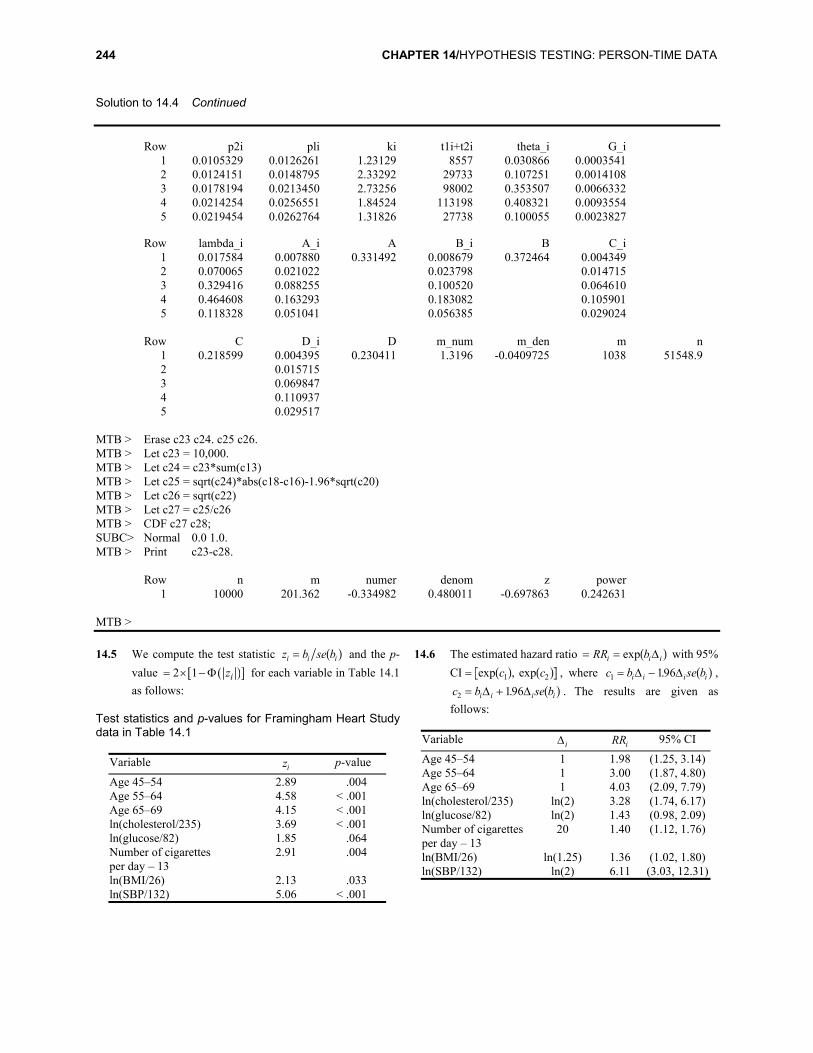
MTB > 14.5 We compute the test statistic z b se bi i i= a f and the p-

value ( )[ ]2 1 iz= × −Φ for each variable in Table 14.1 as follows:

Test statistics and p-values for Framingham Heart Study data in Table 14.1

Variable zi p-value

Age 45–54 2.89 .004 Age 55–64 4.58 < .001 Age 65–69 4.15 < .001 ln(cholesterol/235) 3.69 < .001 ln(glucose/82) 1.85 .064 Number of cigarettes 2.91 .004 per day – 13 ln(BMI/26) 2.13 .033 ln(SBP/132) 5.06 < .001

14.6 The estimated hazard ratio = =RR bi i iexp ∆a f with 95% CI = exp , expc c1 2a f a f , where c b se bi i i i1 196= −∆ ∆. a f , c b se bi i i i2 196= +∆ ∆. a f . The results are given as follows:

Variable ∆i RRi 95% CI

Age 45–54 1 1.98 (1.25, 3.14)Age 55–64 1 3.00 (1.87, 4.80)Age 65–69 1 4.03 (2.09, 7.79)ln(cholesterol/235) ln(2) 3.28 (1.74, 6.17)ln(glucose/82) ln(2) 1.43 (0.98, 2.09)Number of cigarettes 20 1.40 (1.12, 1.76)per day – 13 ln(BMI/26) ln(1.25) 1.36 (1.02, 1.80)ln(SBP/132) ln(2) 6.11 (3.03, 12.31)


The relative risk for age 45–54 represents the hazard for coronary heart disease (CHD) for a 45–54-year-old man compared with a 35–44-year-old man. Thus, the 45–54-year-old man is twice as likely to have a first CHD event over the short term compared with a 35–44-year-old man, all other factors being equal. Similarly, a 55–64-year-old man and a 65–69-year-old man are 3 and 4 times as likely, respectively, to have a first CHD event over the short term compared with a 35–44-year-old man (all other factors being equal). The relative risk of 3.28 for cholesterol represents the hazard ratio for subject A versus subject B, where subject A has double the cholesterol of subject B, all other factors being equal. Since cholesterol is represented on the ln scale, the difference between subject A versus subject B’s ln(cholesterol) level = ln(2). Similarly, the relative risks for glucose and SBP are 1.43 and 6.11, respectively, and represent the comparative hazards for two subjects whose glucose or SBP values are in the ratio of 2:1, all other factors being equal. Furthermore, the relative risk of 1.36 for body mass index (BMI) represents the comparative hazard for two subjects whose BMI values are in the ratio of 1.25:1 (e.g, 25 vs 20 BMI) all other factors being equal. Finally, the relative risk for number of cigarettes per day = 1.40 represents the comparative hazard for two subjects who differ by 1 pack (i.e., 20 cigarettes) per day (e.g., a smoker of 1 pack per day versus a nonsmoker), all other factors being equal.

14.7 The results are very similar to those given in Table

13.18 (text, Chapter 13). A proportional-hazards model is probably more appropriate because it takes into account when an event occurs versus a multiple logistic regression model, which only takes into account whether an event occurs, but not when it occurs. For a relatively rare event such as CHD (163 events out of 1731 subjects), there is not much difference between the two approaches. Another advantage of a proportional-hazards model is the ability to use time-dependent covariates; i.e., covariates that change over time. This is particularly important for risk factors that change a lot over time, such as cigarette-smoking habits. In this example, for simplicity, only fixed covariates defined at baseline were used. In the Framingham Heart Study data set, risk factors are up-dated every 2 years, and therefore it is possible to include time-dependent covariates.

14.8 The number of patrons at the Times Square station in 1992

= ( + FH IK =)260 105 826 105 105 8262

33 070 625, , , , .

The incidence rate per paying patron is

6289 8.74

33,070,625 10= .

A 95% CI for the expected number of events µ( ) is

289 196 289 289 33 3 255 7 322 3± = ± = ( ). . . , . . The corresponding 95% CI for the incidence rate is

255 733 070 625

322 333 070 625

7 7310

9 75106 6

., ,

, ., ,

. , .FH

IK =FH IK .

14.9 The number of paying patrons at the Grand Central

station in 1992

= ( + FH IK =)260 105113 105 1051132

32 847 813, , , , .

The incidence rate per paying patron is

16932 847 813

514106, ,.

= .

A 95% CI for the expected number of events µ( ) is

( )169 1.96 169 169 25.5 143.5, 194.5± = ± = . The corresponding 95% CI for the incidence rate is

6 6143.5 194.5 4.37 5.92, ,

32,847,813 32,847,813 10 10 =

.

14.10 We will use the large-sample procedure given in Equa-

tion 14.8 (text, Chapter 14), since the variance V1 5a f ≥ . We use the test statistic

z a EV

N=− −

( )1 1

1

5 0 1. ~ , under H0


where

a

E

V

1

1

1

289289 169 33 070 625

33 070 625 32 847 813458 502 229 8458 502 498 114 5

=

=+ (

+= ( == ( =

( ) )

)

)( )

, ,, , , ,

. .

. . .

Thus,

z N=− −

= = ( )289 229 8 5

114 558 7310 70

5 49 0 1. ..

.

.. ~ , under H0 .

The p-value = × − ( <)2 1 5 49 001Φ . . . Thus, there is a

significant difference between the felony rates at the two stations.

14.11 We have that RR . . .= =8 74 10 514 10 1706 6b g b g . Further-

more, Var ln .RRd i = + =1 289 1 169 0 00938 . Thus, a 95 % CI for ln RR( ) is

ln . . . . .

. , . .170 196 0 00938 0 530 0190

0 340 0 720( ) ± = ±

= ( )

The corresponding 95% CI for RR is

exp . , exp . . , .0 340 0 720 140 2 05( ) ( ) = ( ). 14.12 You use the station 50 5 2 500× × = times per year.

We will assume that the number of felonies (X) is Poisson-distributed with parameter

µ = FH IK =500 8 7410

0 00446

. . .

We wish to compute

Pr PrX X≥ = − = = − − =( ) ( ) ( )1 1 0 1 0 0044 0044exp . . . 14.13 We will assume that the number of felonies (X) is

Poisson-distributed with parameter

µ = FH IK =500 51410

0 00266

. . .

We wish to compute

Pr PrX X≥ = − = = − −=

( ) ( ) ( )1 1 0 1 0 00260026

exp ..

14.14 The number of paying patrons in 1992 at the Bowery

station

233 260 2332

105 72 813( ) )+ FH IK( = , .

The incidence rate per paying patron

638 521.9

72,813 10= .

We cannot use the large-sample test procedure because

( ) ( )( )

( )( )

1 272,813 33,070,625289 38

72,813 33,070,625327 .0022 .9978 0.72 5.

V

= + +

= = <

Instead, we must use the exact test given in Equa-

tion 14.9 (text, Chapter 14). We have

( ) ( )

( ) ( )

327327

38327

327

38

327-value 2 .0022 .9978

3272 1 .0022 .9978

k k

k

k k

k

pk

k

−

=

−

=

=

= −

∑

∑

We use the BINOMDIST function of Excel to evaluate

this expression. We have

Pr x n p≤ = =( ) =3 327 0022 9938, . . . Thus,

Pr PrX X≥ = − ≤ = − =( ) ( )4 1 3 1 9938 0062. . . Since Pr PrX X≥ ≤ ≥ =( ) ( )38 4 0062. , it follows that we

can reject H0 and conclude that the incidence rate of felonies is significantly higher at the Bowery station.

14.15 The estimated rate ratio

(RR) = =521108 7410

6

6

59 7.9

.. .

Thus, a patron is about 60 times as likely to be a

felony victim at the Bowery station than at the Times Square station. Indeed, if a patron uses the Bowery station every workday, twice a day, for a year (i.e., 50 5 2 500× × = times, allowing for a 2-week vaca-tion), then the probability of at least one felony

= ≥ = − = = − −( )( ) ( )Pr PrX X1 1 0 1 exp µ .

In this case, µ = =500 5219 10 0 26096. .a f . Thus,

Pr X ≥ = − − =( ) ( )1 1 0 2609 230exp . . ! Thus, there is a 23% probability of being a felony victim over a 1-year period at the Bowery station versus a 0.4% probability at the Times Square station. Clearly, the Bowery station is more dangerous.

14.16 We use the test for trend for incidence-rate data given

in Equation 14.37 (text, Chapter 14). We assume a model of the form


ln p Sij i jc h = +α β where

p i

jS j

j

ij

j

=

=

=

incidence rate in the th age group

and the th age at 1st birth groupscore for the th age at 1st birth group,

1 6, ,…

We will use scores of 1, ... , 6 for the age at 1st birth

groups = < 20, 20–24, 25–29, 30–34, 35–39, and 40+, respectively. We wish to test the hypothesis

H0 : β = 0 versus H1 : β ≠ 0 .

We use the test statistic z se N= ~ ,β βe j a f0 1 under

H0 . We estimate β with the ith age group by

, ,i xy i xx iL Lβ = , where

( )( )

6

6 61

, 61 1

126

612

, 61

1

ˆlnˆln

ij ijj

xy i ij j ij ij jj j

ijj

ij jj

xx i ij jj

ijj

a p

L a S p a Sa

a S

L a Sa

=

= =

=

=

=

=

= − ×

= −

∑∑ ∑

∑

∑∑

∑

aij = number of breast cancer cases within the ith age

group and jth age at 1st birth group

The ( ) ( )1 2,

ˆ 1i xx ise Lβ = , with test statistic

( ) ( )ˆ ˆ 0,1i i iz se Nβ β= ∼ under H0 with p-value

( )[ ]2 1 iz= × −Φ . To obtain an overall estimate of the slope, we compute

4 4

, ,1 1

ˆxy i xx i

i i

L Lβ= =

= ∑ ∑ with standard error equal to

( )1 24

,1

ˆ 1 xx ii

se Lβ=

= ∑ . The corresponding test

statistic is ( ) ( )ˆ ˆ 0,1z se Nβ β= ∼ under H0. The

two-sided ( )[ ]-value 2 1p z= × −Φ . The estimated slope within each age group and overall is given in the Excel spreadsheet shown on the following page. We see that ˆ 0.184β = , ( )ˆ 0.026se β = , 7.16z = . Clearly,

the p-value ( )[ ]2 1 .001z= −Φ < . Thus, among parous women, there is a significant relationship between breast-cancer incidence and age at 1st birth with breast cancer incidence increasing as age at 1st birth increases.

14.17 The estimated percentage increase in breast-cancer

incidence for every 5-year increase in age at 1st birth

( )ˆ exp 0.184 20.2%= ∆ = = . A 95% CI for ∆ = exp , expc c1 2a f a f where

( ) ( )

( )1

2

ˆ ˆ1.96 0.184 1.96 0.026 0.133

0.184 1.96 0.026 0.235

c se

c

β β= − = − =

= + =

Thus, the 95% CI for ∆ is

( ) ( )[ ] ( )exp 0.133 , exp 0.235 14.2%, 26.5%= .


Solution to 14.16 Age Group = 30-39 Age at 1st birth

Score ( )Sij ija person-

years incidence ij ija S 2ij ija S xxL ( )lnij ija p ( )lnij ij ija S p xyL Beta se z p-value

< 20 1 3 1067 0.002812 3 3 -17.62 -17.62 20-24 2 62 97140 0.000638 124 248 -456.12 -912.24 25-29 3 73 82959 0.00088 219 657 -513.60 -1540.81 30-34 4 11 11879 0.000926 44 176 -76.83 -307.32 35-39 5 1 937 0.001067 5 25 -6.84 -34.21

150 395 1109 68.83 -1071.02 -2812.20 8.14 0.118 0.121 0.981 .326

Age Group = 40-49 Age at 1st birth



< 20 1 3 2381 0.00126 3 3 -20.03 -20.03 20-24 2 349 218239 0.001599 698 1396 -2246.96 -4493.92 25-29 3 290 173714 0.001669 870 2610 -1854.63 -5563.90 30-34 4 73 32895 0.002219 292 1168 -446.08 -1784.30 35-39 5 16 6264 0.002554 80 400 -95.52 -477.60 40-44 6 3 813 0.00369 18 108 -16.81 -100.84

734 1961 5685 445.87 -4680.02 -12440.58 62.86 0.141 0.047 2.977 .003




< 20 1 3 1693 0.001772 3 3 -19.01 -19.01 20-24 2 327 156907 0.002084 654 1308 -2018.72 -4037.44 25-29 3 454 181244 0.002505 1362 4086 -2719.23 -8157.70 30-34 4 133 43721 0.003042 532 2128 -770.77 -3083.06 35-39 5 43 11291 0.003808 215 1075 -239.53 -1197.67 40-44 6 13 2341 0.005553 78 468 -67.51 -405.08

973 2844 9068 755.22 -5834.77 -16899.96 154.6 0.205 0.036 5.626 .000




< 20 1 3 261 0.011494 3 3 -13.40 -13.40 20-24 2 72 30214 0.002383 144 288 -434.84 -869.67 25-29 3 148 53486 0.002767 444 1332 -871.71 -2615.14 30-34 4 67 15319 0.004374 268 1072 -363.95 -1455.82 35-39 5 21 4057 0.005176 105 525 -110.54 -552.69 40-44 6 1 877 0.00114 6 36 -6.78 -40.66

312 970 3256 240.29 -1801.22 -5547.38 52.56 .219 .065 3.391 .001

Overall 2169 1510.22 278.16 0.184 0.026 7.158 .000

REFERENCE ...................................................................................................................

[1] New York Post, August 30, 1993, p. 4.

hypothesis esting: person-time data chapter 14.pdf · section 14.1 measures of effect for...

Documents