hyperbolic geometry - brown universityrkenyon/papers/cannon.pdf · hyperbolic geometry james w....
TRANSCRIPT
Flavors of GeometryMSRI PublicationsVolume 31, 1997
Hyperbolic Geometry
JAMES W. CANNON, WILLIAM J. FLOYD, RICHARD KENYON,
AND WALTER R. PARRY
Contents
1. Introduction 592. The Origins of Hyperbolic Geometry 603. Why Call it Hyperbolic Geometry? 634. Understanding the One-Dimensional Case 655. Generalizing to Higher Dimensions 676. Rudiments of Riemannian Geometry 687. Five Models of Hyperbolic Space 698. Stereographic Projection 729. Geodesics 7710. Isometries and Distances in the Hyperboloid Model 8011. The Space at Infinity 8412. The Geometric Classification of Isometries 8413. Curious Facts about Hyperbolic Space 8614. The Sixth Model 9515. Why Study Hyperbolic Geometry? 9816. When Does a Manifold Have a Hyperbolic Structure? 10317. How to Get Analytic Coordinates at Infinity? 106References 108Index 110
1. Introduction
Hyperbolic geometry was created in the first half of the nineteenth century
in the midst of attempts to understand Euclid’s axiomatic basis for geometry.
It is one type of non-Euclidean geometry, that is, a geometry that discards one
of Euclid’s axioms. Einstein and Minkowski found in non-Euclidean geometry a
This work was supported in part by The Geometry Center, University of Minnesota, an STC
funded by NSF, DOE, and Minnesota Technology, Inc., by the Mathematical Sciences Research
Institute, and by NSF research grants.
59
60 J. W. CANNON, W. J. FLOYD, R. KENYON, AND W. R. PARRY
geometric basis for the understanding of physical time and space. In the early
part of the twentieth century every serious student of mathematics and physics
studied non-Euclidean geometry. This has not been true of the mathematicians
and physicists of our generation. Nevertheless with the passage of time it has
become more and more apparent that the negatively curved geometries, of which
hyperbolic non-Euclidean geometry is the prototype, are the generic forms of ge-
ometry. They have profound applications to the study of complex variables, to
the topology of two- and three-dimensional manifolds, to the study of finitely
presented infinite groups, to physics, and to other disparate fields of mathemat-
ics. A working knowledge of hyperbolic geometry has become a prerequisite for
workers in these fields.
These notes are intended as a relatively quick introduction to hyperbolic ge-
ometry. They review the wonderful history of non-Euclidean geometry. They
give five different analytic models for and several combinatorial approximations
to non-Euclidean geometry by means of which the reader can develop an intu-
ition for the behavior of this geometry. They develop a number of the properties
of this geometry that are particularly important in topology and group theory.
They indicate some of the fundamental problems being approached by means of
non-Euclidean geometry in topology and group theory.
Volumes have been written on non-Euclidean geometry, which the reader
must consult for more exhaustive information. We recommend [Iversen 1993]
for starters, and [Benedetti and Petronio 1992; Thurston 1997; Ratcliffe 1994]
for more advanced readers. The latter has a particularly comprehensive bibliog-
raphy.
2. The Origins of Hyperbolic Geometry
Except for Euclid’s five fundamental postulates of plane geometry, which we
paraphrase from [Kline 1972], most of the following historical material is taken
from Felix Klein’s book [1928]. Here are Euclid’s postulates in contemporary
language (compare [Euclid 1926]):
1. Each pair of points can be joined by one and only one straight line segment.
2. Any straight line segment can be indefinitely extended in either direction.
3. There is exactly one circle of any given radius with any given center.
4. All right angles are congruent to one another.
5. If a straight line falling on two straight lines makes the interior angles on
the same side less than two right angles, the two straight lines, if extended
indefinitely, meet on that side on which the angles are less than two right
angles.
Of these five postulates, the fifth is by far the most complicated and unnatural.
Given the first four, the fifth postulate can easily be seen to be equivalent to the

HYPERBOLIC GEOMETRY 61
following parallel postulate, which explains why the expressions “Euclid’s fifth
postulate” and “the parallel parallel” are often used interchangeably:
5′. Given a line and a point not on it, there is exactly one line going through
the given point that is parallel to the given line.
For two thousand years mathematicians attempted to deduce the fifth postulate
from the four simpler postulates. In each case one reduced the proof of the
fifth postulate to the conjunction of the first four postulates with an additional
natural postulate that, in fact, proved to be equivalent to the fifth:
Proclus (ca. 400 a.d.) used as additional postulate the assumption that the
points at constant distance from a given line on one side form a straight line.
The Englishman John Wallis (1616–1703) used the assumption that to every
triangle there is a similar triangle of each given size.
The Italian Girolamo Saccheri (1667–1733) considered quadrilaterals with two
base angles equal to a right angle and with vertical sides having equal length and
deduced consequences from the (non-Euclidean) possibility that the remaining
two angles were not right angles.
Johann Heinrich Lambert (1728–1777) proceeded in a similar fashion and
wrote an extensive work on the subject, posthumously published in 1786.
Gottingen mathematician Kastner (1719–1800) directed a thesis of student
Klugel (1739–1812), which considered approximately thirty proof attempts for
the parallel postulate.
Decisive progress came in the nineteenth century, when mathematicians aban-
doned the effort to find a contradiction in the denial of the fifth postulate and
instead worked out carefully and completely the consequences of such a denial.
It was found that a coherent theory arises if instead one assumes that
Given a line and a point not on it, there is more than one line going through
the given point that is parallel to the given line.
This postulate is to hyperbolic geometry as the parallel postulate 5′ is to Eu-
clidean geometry.
Unusual consequences of this change came to be recognized as fundamental
and surprising properties of non-Euclidean geometry: equidistant curves on ei-
ther side of a straight line were in fact not straight but curved; similar triangles
were congruent; angle sums in a triangle were not equal to π, and so forth.
That the parallel postulate fails in the models of non-Euclidean geometry
that we shall give will be apparent to the reader. The unusual properties of non-
Euclidean geometry that we have mentioned will all be worked out in Section 13,
entitled “Curious facts about hyperbolic space”.
History has associated five names with this enterprise, those of three profes-
sional mathematicians and two amateurs.
The amateurs were jurist Schweikart and his nephew Taurinus (1794–1874).
By 1816 Schweikart had developed, in his spare time, an “astral geometry” that
62 J. W. CANNON, W. J. FLOYD, R. KENYON, AND W. R. PARRY
was independent of the fifth postulate. His nephew Taurinus had attained a
non-Euclidean hyperbolic geometry by the year 1824.
The professionals were Carl Friedrich Gauss (1777–1855), Nikolaı Ivanovich
Lobachevskiı (1793–1856), and Janos (or Johann) Bolyai (1802–1860). From
the papers of his estate it is apparent that Gauss had considered the parallel
postulate extensively during his youth and at least by the year 1817 had a clear
picture of non-Euclidean geometry. The only indications he gave of his knowledge
were small comments in his correspondence. Having satisfied his own curiosity,
he was not interested in defending the concept in the controversy that was sure
to accompany its announcement. Bolyai’s father Farkas (or Wolfgang) (1775–
1856) was a student friend of Gauss and remained in correspondence with him
throughout his life. Farkas devoted much of his life’s effort unsuccessfully to
the proof of the parallel postulate and consequently tried to turn his son away
from its study. Nevertheless, Janos attacked the problem with vigor and had
constructed the foundations of hyperbolic geometry by the year 1823. His work
appeared in 1832 or 1833 as an appendix to a textbook written by his father.
Lobachevskiı also developed a non-Euclidean geometry extensively and was, in
fact, the first to publish his findings, in 1829. See [Lobachevskiı 1898; Bolyai
and Bolyai 1913].
Gauss, the Bolyais, and Lobachevskiı developed non-Euclidean geometry ax-
iomatically on a synthetic basis. They had neither an analytic understanding
nor an analytic model of non-Euclidean geometry. They did not prove the
consistency of their geometries. They instead satisfied themselves with the
conviction they attained by extensive exploration in non-Euclidean geometry
where theorem after theorem fit consistently with what they had discovered to
date. Lobachevskiı developed a non-Euclidean trigonometry that paralleled the
trigonometric formulas of Euclidean geometry. He argued for the consistency
based on the consistency of his analytic formulas.
The basis necessary for an analytic study of hyperbolic non-Euclidean geom-
etry was laid by Leonhard Euler, Gaspard Monge, and Gauss in their studies
of curved surfaces. In 1837 Lobachevskiı suggested that curved surfaces of con-
stant negative curvature might represent non-Euclidean geometry. Two years
later, working independently and largely in ignorance of Lobachevskiı’s work,
yet publishing in the same journal, Minding made an extensive study of surfaces
of constant curvature and verified Lobachevskiı suggestion. Bernhard Riemann
(1826–1866), in his vast generalization [Riemann 1854] of curved surfaces to the
study of what are now called Riemannian manifolds, recognized all of these rela-
tionships and, in fact, to some extent used them as a springboard for his studies.
All of the connections among these subjects were particularly pointed out by Eu-
genio Beltrami in 1868. This analytic work provided specific analytic models for
non-Euclidean geometry and established the fact that non-Euclidean geometry
was precisely as consistent as Euclidean geometry itself.
HYPERBOLIC GEOMETRY 63
We shall consider in this exposition five of the most famous of the analytic
models of hyperbolic geometry. Three are conformal models associated with the
name of Henri Poincare. A conformal model is one for which the metric is a
point-by-point scaling of the Euclidean metric. Poincare discovered his models
in the process of defining and understanding Fuchsian, Kleinian, and general
automorphic functions of a single complex variable. The story is one of the most
famous and fascinating stories about discovery and the work of the subconscious
mind in all of science. We quote from [Poincare 1908]:
For fifteen days I strove to prove that there could not be any functions like
those I have since called Fuchsian functions. I was then very ignorant; every
day I seated myself at my work table, stayed an hour or two, tried a great
number of combinations and reached no results. One evening, contrary
to my custom, I drank black coffee and could not sleep. Ideas rose in
crowds; I felt them collide until pairs interlocked, so to speak, making a
stable combination. By the next morning I had established the existence
of a class of Fuchsian functions, those which come from the hypergeometric
series; I had only to write out the results, which took but a few hours.
Then I wanted to represent these functions by the quotient of two series;
this idea was perfectly conscious and deliberate, the analogy with elliptic
functions guided me. I asked myself what properties these series must have
if they existed, and I succeeded without difficulty in forming the series I
have called theta-Fuchsian.
Just at this time I left Caen, where I was then living, to go on a geological
excursion under the auspices of the school of mines. The changes of travel
made me forget my mathematical work. Having reached Coutances, we
entered an omnibus to go some place or other. At the moment when I put
my foot on the step the idea came to me, without anything in my former
thoughts seeming to have paved the way for it, that the transformations I
had used to define the Fuchsian functions were identical with those of non-
Euclidean geometry. I did not verify the idea; I should not have had time,
as, upon taking my seat in the omnibus, I went on with a conversation
already commenced, but I felt a perfect certainty. On my return to Caen,
for conscience’ sake I verified the result at my leisure.
3. Why Call it Hyperbolic Geometry?
The non-Euclidean geometry of Gauss, Lobachevskiı, and Bolyai is usually
called hyperbolic geometry because of one of its very natural analytic models.
We describe that model here.
Classically, space and time were considered as independent quantities; an
event could be given coordinates (x1, . . . , xn+1) ∈ � n+1 , with the coordinate
xn+1 representing time, and the only reasonable metric was the Euclidean metric
with the positive definite square-norm x21 + · · · + x2
n+1.
64 J. W. CANNON, W. J. FLOYD, R. KENYON, AND W. R. PARRY
↑
↑
↑
x
x′
hyperbolic space
light cone
projective identification x = x′
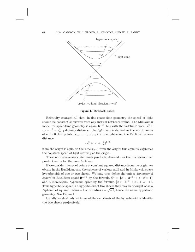
Figure 1. Minkowski space.
Relativity changed all that; in flat space-time geometry the speed of light
should be constant as viewed from any inertial reference frame. The Minkowski
model for space-time geometry is again� n+1 but with the indefinite norm x2
1 +
· · · + x2n − x2
n+1 defining distance. The light cone is defined as the set of points
of norm 0. For points (x1, . . . , xn, xn+1) on the light cone, the Euclidean space-
distance
(x21 + · · · + x2
n)1/2
from the origin is equal to the time xn+1 from the origin; this equality expresses
the constant speed of light starting at the origin.
These norms have associated inner products, denoted · for the Euclidean inner
product and ∗ for the non-Euclidean.
If we consider the set of points at constant squared distance from the origin, we
obtain in the Euclidean case the spheres of various radii and in Minkowski space
hyperboloids of one or two sheets. We may thus define the unit n-dimensional
sphere in Euclidean space� n+1 by the formula Sn = {x ∈ � n+1 : x · x = 1}
and n-dimensional hyperbolic space by the formula {x ∈ � n+1 : x ∗ x = −1}.Thus hyperbolic space is a hyperboloid of two sheets that may be thought of as a
“sphere” of squared radius −1 or of radius i =√−1; hence the name hyperbolic
geometry. See Figure 1.
Usually we deal only with one of the two sheets of the hyperboloid or identify
the two sheets projectively.

HYPERBOLIC GEOMETRY 65
general path
p(t) = (x(t), y(t))
p′(t)
path of speed 1
p′(t) = (− sin t, cos t)
p(t) = (cos t, sin t)
k = 1t = arc length
Figure 2. The circle S1.
4. Understanding the One-Dimensional Case
The key to understanding hyperbolic spaceHn and its intrinsic metric coming
from the indefinite Minkowski inner product ∗ is to first understand the case
n = 1. We argue by analogy with the Euclidean case and prepare the analogy
by recalling the familiar Euclidean case of the circle S1.
Let p : (−∞,∞) → S1 be a smooth path with p(0) = (1, 0). If we write
in coordinates p(t) = (x(t), y(t)) where x2 + y2 = 1, then differentiating this
equation we find
2x(t)x′(t) + 2y(t)y′(t) = 0,
or in other words p(t) · p′(t) = 0. That is, the velocity vector p′(t) is Euclidean-
perpendicular to the position vector p(t). In particular we may write p′(t) =
k(t)(−y(t), x(t)), since the tangent space to S1 at p(t) is one-dimensional and
(−y(t), x(t)) is Euclidean-perpendicular to p = (x, y). See Figure 2.
If we assume in addition that p(t) has constant speed 1, then
1 = |p′(t)| = |k(t)|√
(−y)2 + x2 = |k(t)|,
and so k ≡ ±1. Taking k ≡ 1, we see that p = (x, y) travels around the unit circle
in the Euclidean plane at constant speed 1. Consequently we may by definition
identify t with Euclidean arclength on the unit circle, x = x(t) with cos t and
y = y(t) with sin t, and we see that we have given a complete proof of the fact
from beginning calculus that the derivative of the cosine is minus the sine and
that the derivative of the sine is the cosine, a proof that is conceptually simpler
than the proofs usually given in class.
In formulas, taking k = 1, we have shown that x and y (the cosine and sine)
satisfy the system of differential equations
x′(t) = −y(t), y′(t) = x(t),
with initial conditions x(0) = 1, y(0) = 0. We then need only apply some
elementary method such as the method of undetermined coefficients to easily
66 J. W. CANNON, W. J. FLOYD, R. KENYON, AND W. R. PARRY
discover the classical power series for the sine and cosine:
cos t = 1 − t2/2! + t4/4!− · · · ,sin t = t− t3/3! + t5/5!− · · · .
The hyperbolic calculation in H1 requires only a new starting point (0, 1)
instead of (1, 0), the replacement of S1 by H1, the replacement of the Euclidean
inner product · by the hyperbolic inner product ∗, an occasional replacement
of +1 by −1, the replacement of Euclidean arclength by hyperbolic arclength,
the replacement of cosine by hyperbolic sine, and the replacement of sine by the
hyperbolic cosine. Here is the calculation.
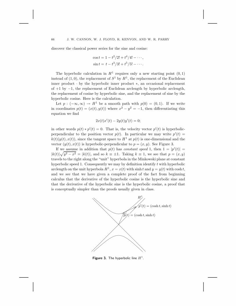
Let p : (−∞,∞) → H1 be a smooth path with p(0) = (0, 1). If we write
in coordinates p(t) = (x(t), y(t)) where x2 − y2 = −1, then differentiating this
equation we find
2x(t)x′(t) − 2y(t)y′(t) = 0;
in other words p(t) ∗ p′(t) = 0. That is, the velocity vector p′(t) is hyperbolic-
perpendicular to the position vector p(t). In particular we may write p′(t) =
k(t)(y(t), x(t)), since the tangent space to H1 at p(t) is one-dimensional and the
vector (y(t), x(t)) is hyperbolic-perpendicular to p = (x, y). See Figure 3.
If we assume in addition that p(t) has constant speed 1, then 1 = |p′(t)| =
|k(t)|√
y2 − x2 = |k(t)|, and so k ≡ ±1. Taking k ≡ 1, we see that p = (x, y)
travels to the right along the “unit” hyperbola in the Minkowski plane at constant
hyperbolic speed 1. Consequently we may by definition identify t with hyperbolic
arclength on the unit hyperbolaH1, x = x(t) with sinh t and y = y(t) with cosh t,
and we see that we have given a complete proof of the fact from beginning
calculus that the derivative of the hyperbolic cosine is the hyperbolic sine and
that the derivative of the hyperbolic sine is the hyperbolic cosine, a proof that
is conceptually simpler than the proofs usually given in class.
p(t) = (cosh t, sinh t)
p′(t) = (cosh t, sinh t)
H1
Figure 3. The hyperbolic line H1.

HYPERBOLIC GEOMETRY 67
In formulas, taking k = 1, we have shown that x and y (the hyperbolic sine
and cosine) satisfy the system of differential equations
x′(t) = y(t), y′(t) = x(t),
with initial conditions x(0) = 0, y(0) = 1. We then need only apply some
elementary method such as the method of undetermined coefficients to easily
discover the classical power series for the hyperbolic sine and cosine:
cosh t = 1 + t2/2! + t4/4! + · · · ,sinh t = t+ t3/3! + t5/5! + · · · .
It seems to us a shame that these analogies, being as easy as they are, are
seldom developed in calculus classes. The reason of course is that the analogies
become forced if one is not willing to leave the familiar Euclidean plane for the
unfamiliar Minkowski plane.
Note the remarkable fact that our calculation showed that a nonzero tangent
vector toH1 has positive square norm with respect to the indefinite inner product
∗; that is, the indefinite inner product on the Minkowski plane restricts to a
positive definite inner product on hyperbolic one-space. We shall find that the
analogous result is true in higher dimensions and that the formulas we have
calculated for hyperbolic length in dimension one apply in the higher-dimensional
setting as well.
5. Generalizing to Higher Dimensions
In higher dimensions, Hn sits inside� n+1 as a hyperboloid. If p : (−∞,∞) →
Hn again describes a smooth path, then from the defining equations we still have
p(t)∗p′(t) = 0. By taking paths in any direction running through the point p(t),
we see that the tangent vectors to Hn at p(t) form the hyperbolic orthogonal
complement to the vector p(t) (vectors are hyperbolically orthogonal if their
inner product with respect to ∗ is 0).
We can show that the form ∗ restricted to the tangent space is positive definite
in either of two instructive ways.
The first method uses the Cauchy–Schwarz inequality (x · y)2 ≤ (x · x)(y · y).Suppose that p = (p, pn+1) is in Hn and x = (x, xn+1) 6= 0 is in the tangent
space of Hn at p, where p, x ∈ � n . If xn+1 = 0, then x∗x = x ·x. Hence x∗x > 0
if xn+1 = 0, so we may assume that xn+1 6= 0. Then 0 = x∗p = x · p−xn+1pn+1,
and −1 = p ∗ p = p · p− p2n+1. Hence, Cauchy–Schwarz gives
(x · x)(p · p) ≥ (x · p)2 = (xn+1pn+1)2 = x2
n+1(p · p+ 1).
Therefore, (x ∗ x)(p · p) ≥ x2n+1, which implies x ∗ x > 0 if x 6= 0.
The second method analyzes the inner product ∗ algebraically. (For complete
details, see [Weyl 1919], for example.) Take a basis p, p1, . . . , pn for� n+1 where
p is the point of interest in Hn and the remaining vectors span the n-dimensional

68 J. W. CANNON, W. J. FLOYD, R. KENYON, AND W. R. PARRY
tangent space to Hn at p. Now apply the Gram–Schmidt orthogonalization pro-
cess to this basis. Since p ∗ p = −1 by the defining equation for Hn, the vector
p, being already a unit vector, is unchanged by the process and the remainder of
the resulting basis spans the orthogonal complement of p, which is the tangent
space to Hn at p. Since the inner product ∗ is nondegenerate, the resulting ma-
trix is diagonal with entries of ±1 on the diagonal, one of the −1’s corresponding
to the vector p. By Sylvester’s theorem of inertia, the number of +1’s and −1’s
on the diagonal is an invariant of the inner product (the number of 1’s is the
dimension of the largest subspace on which the metric is positive definite). But
with the standard basis for� n+1 , there is exactly one −1 on the diagonal and
the remaining entries are +1. Hence the same is true of our basis. Thus the
matrix of the inner product when restricted to our tangent space is the identity
matrix of order n; that is, the restriction of the metric to the tangent space is
positive definite.
Thus the inner product ∗ restricted to Hn defines a genuine Riemannian
metric on Hn.
6. Rudiments of Riemannian Geometry
Our analytic models of hyperbolic geometry will all be differentiable manifolds
with a Riemannian metric.
One first defines a Riemannian metric and associated geometric notions on
Euclidean space. A Riemannian metric ds2 on Euclidean space� n is a function
that assigns at each point p ∈ � n a positive definite symmetric inner product on
the tangent space at p, this inner product varying differentiably with the point
p. Given this inner product, it is possible to define any number of standard
geometric notions such as the length |x| of a vector x, where |x|2 = x·x, the angle
θ between two vectors x and y, where cos θ = (x ·y)/(|x| · |y|), the length element
ds =√ds2, and the area element dA, where dA is calculated as follows: if x1, . . . ,
xn are the standard coordinates on� n , then ds2 has the form
∑
i,j gij dxi dxj ,
and the matrix (gij) depends differentiably on x and is positive definite and
symmetric. Let√
|g| denote the square root of the determinant of (gij). Then
dA =√
|g| dx1 dx2 · · · dxn. If f :� k → � n is a differentiable map, one can
define the pullback f∗(ds2) by the formula
f∗(ds2)(v, w) = ds2(Df(v), Df(w))
where v and w are tangent vectors at a point u of� k and Df is the derivative
map that takes tangent vectors at u to tangent vectors at x = f(u). One can
also calculate the pullback formally by replacing gij(x) with x ∈ � n by gij ◦f(u),
where u ∈ � k and f(u) = x, and replacing dxi by∑
j(∂fi/∂uj)duj . One can
HYPERBOLIC GEOMETRY 69
p∗(ds)
ds
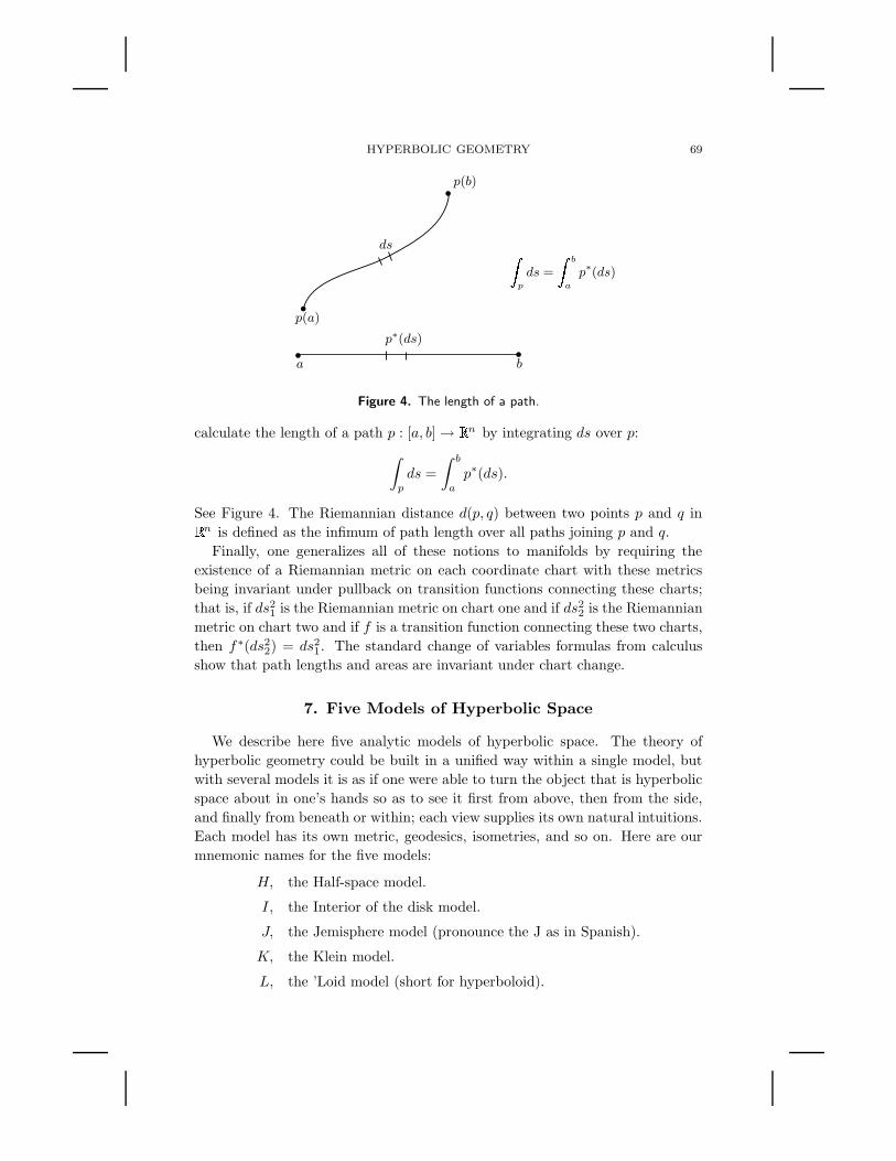
p(b)
p(a)
ba
�p
ds =
� b
a
p∗(ds)
Figure 4. The length of a path.
calculate the length of a path p : [a, b] → � n by integrating ds over p:
∫
p
ds =
∫ b
a
p∗(ds).
See Figure 4. The Riemannian distance d(p, q) between two points p and q in� n is defined as the infimum of path length over all paths joining p and q.
Finally, one generalizes all of these notions to manifolds by requiring the
existence of a Riemannian metric on each coordinate chart with these metrics
being invariant under pullback on transition functions connecting these charts;
that is, if ds21 is the Riemannian metric on chart one and if ds22 is the Riemannian
metric on chart two and if f is a transition function connecting these two charts,
then f∗(ds22) = ds21. The standard change of variables formulas from calculus
show that path lengths and areas are invariant under chart change.
7. Five Models of Hyperbolic Space
We describe here five analytic models of hyperbolic space. The theory of
hyperbolic geometry could be built in a unified way within a single model, but
with several models it is as if one were able to turn the object that is hyperbolic
space about in one’s hands so as to see it first from above, then from the side,
and finally from beneath or within; each view supplies its own natural intuitions.
Each model has its own metric, geodesics, isometries, and so on. Here are our
mnemonic names for the five models:
H, the Half-space model.
I, the Interior of the disk model.
J, the Jemisphere model (pronounce the J as in Spanish).
K, the Klein model.
L, the ’Loid model (short for hyperboloid).

70 J. W. CANNON, W. J. FLOYD, R. KENYON, AND W. R. PARRY
H
L
J
K k
l
j
i
h
(0, 0)(−1, 0)
(0,−1)
I
Figure 5. The five analytic models and their connecting isometries. The points
h ∈ H, i ∈ I, j ∈ J , k ∈ K, and l ∈ L can be thought of as the same point in
(synthetic) hyperbolic space.
Each model is defined on a different subset of� n+1 , called its domain; for
n = 1 these sets are schematically indicated in Figure 5, which can also be
regarded as a cross section of the picture in higher dimensions. Here are the
definitions of the five domains:
H = {(1, x2, . . . , xn+1) : xn+1 > 0};I = {(x1, . . . , xn, 0) : x2
1 + · · · + x2n < 1};
J = {(x1, . . . , xn+1) : x21 + · · · + x2
n+1 = 1 and xn+1 > 0};K = {(x1, . . . , xn, 1) : x2
1 + · · · + x2n < 1};
L = {(x1, . . . , xn, xn+1) : x21 + · · · + x2
n − x2n+1 = −1 and xn+1 > 0}.

HYPERBOLIC GEOMETRY 71
The associated Riemannian metrics ds2 that complete the analytic description
of the five models are:
ds2H =dx2
2 + · · · + dx2n+1
x2n+1
;
ds2I = 4dx2
1 + · · · + dx2n
(1 − x21 − · · · − x2
n)2;
ds2J =dx2
1 + · · · + dx2n+1
x2n+1
;
ds2K =dx2
1 + · · · + dx2n
(1 − x21 − · · · − x2
n)+
(x1 dx1 + · · · + xn dxn)2
(1 − x21 − · · · − x2
n)2;
ds2L = dx21 + · · · + dx2
n − dx2n+1.
To see that these five models are isometrically equivalent, we need to describe
isometries among them. We use J as the central model and describe for each of
the others a simple map to or from J .
The map α : J → H is central projection from the point (−1, 0, . . . , 0):
α : J → H, (x1, . . . , xn+1) 7→ (1, 2x2/(x1 + 1), . . . , 2xn+1/(x1 + 1)).
The map β : J → I is central projection from (0, . . . , 0,−1):
β : J → I, (x1, . . . , xn+1) 7→ (x1/(xn+1 + 1), . . . , xn/(xn+1 + 1), 0).
The map γ : K → J is vertical projection:
γ : K → J, (x1, . . . , xn, 1) 7→(
x1, . . . , xn,√
1 − x21 − · · · − x2
n
)
.
The map δ : L→ J is central projection from (0, . . . , 0,−1):
δ : L→ J, (x1, . . . , xn+1) 7→ (x1/xn+1, . . . , xn/xn+1, 1/xn+1).
Each map can be used in the standard way to pull back the Riemannian metric
from the target domain to the source domain and to verify thereby that the maps
are isometries. Among the twenty possible connecting maps among our models,
we have chosen the four for which we find the calculation of the metric pullback
easiest. It is worth noting that the metric on the Klein model K, which has
always struck us as particularly ugly and unintuitive, takes on obvious meaning
and structure relative to the metric on J from which it naturally derives via
the connecting map γ : K → J . We perform here two of the four pullback
calculations as examples and recommend that the reader undertake the other
two.
Here is the calculation that shows that α∗(ds2H ) = ds2J . Set
y2 = 2x2/(x1 + 1), . . . , yn+1 = 2xn+1/(x1 + 1).
Then
dyi =2
x1 + 1(dxi −
xi
x1 + 1dx1).
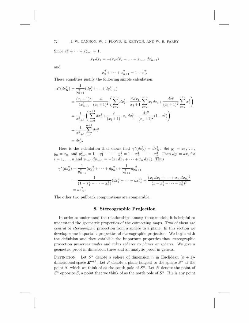
72 J. W. CANNON, W. J. FLOYD, R. KENYON, AND W. R. PARRY
Since x21 + · · · + x2
n+1 = 1,
x1 dx1 = −(x2 dx2 + · · · + xn+1 dxn+1)
and
x22 + · · · + x2
n+1 = 1 − x21.
These equalities justify the following simple calculation:
α∗(ds2H) =1
y2n+1
(dy22 + · · ·+dy2
n+1)
=(x1 +1)2
4x2n+1
4
(x1 +1)2
( n+1∑
i=2
dx2i −
2dx1
x1 +1
n+1∑
i=2
xi dxi +dx2
1
(x1 +1)2
n+1∑
i=2
x2i
)
=1
x2n+1
( n+1∑
i=2
dx2i +
2
(x1 +1)·x1 dx
21 +
dx21
(x1 +1)2(1−x2
1)
)
=1
x2n+1
n+1∑
i=1
dx2i
= ds2J .
Here is the calculation that shows that γ∗(ds2J ) = ds2K . Set y1 = x1, . . . ,
yn = xn, and y2n+1 = 1 − y2
1 − · · · − y2n = 1 − x2
1 − · · · − x2n. Then dyi = dxi for
i = 1, . . . , n and yn+1 dyn+1 = −(x1 dx1 + · · · + xn dxn). Thus
γ∗(ds2J ) =1
y2n+1
(dy21 + · · · + dy2
n) +1
y2n+1
dy2n+1
=1
(1 − x21 − · · · − x2
n)(dx2
1 + · · · + dx2n) +
(x1 dx1 + · · · + xn dxn)2
(1 − x21 − · · · − x2
n)2
= ds2K .
The other two pullback computations are comparable.
8. Stereographic Projection
In order to understand the relationships among these models, it is helpful to
understand the geometric properties of the connecting maps. Two of them are
central or stereographic projection from a sphere to a plane. In this section we
develop some important properties of stereographic projection. We begin with
the definition and then establish the important properties that stereographic
projection preserves angles and takes spheres to planes or spheres. We give a
geometric proof in dimension three and an analytic proof in general.
Definition. Let Sn denote a sphere of dimension n in Euclidean (n + 1)-
dimensional space� n+1 . Let P denote a plane tangent to the sphere Sn at the
point S, which we think of as the south pole of Sn. Let N denote the point of
Sn opposite S, a point that we think of as the north pole of Sn. If x is any point
HYPERBOLIC GEOMETRY 73
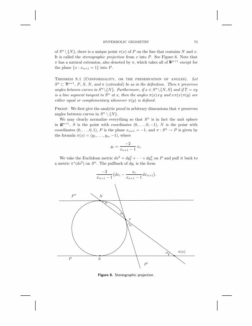
of Sn \{N}, there is a unique point π(x) of P on the line that contains N and x.
It is called the stereographic projection from x into P . See Figure 6. Note that
π has a natural extension, also denoted by π, which takes all of� n+1 except for
the plane {x : xn+1 = 1} into P .
Theorem 8.1 (Conformality, or the preservation of angles). Let
Sn ⊂ � n+1 , P , S, N , and π (extended) be as in the definition. Then π preserves
angles between curves in Sn\{N}. Furthermore, if x ∈ Sn\{N,S} and if T = xy
is a line segment tangent to Sn at x, then the angles π(x)xy and xπ(x)π(y) are
either equal or complementary whenever π(y) is defined .
Proof. We first give the analytic proof in arbitrary dimensions that π preserves
angles between curves in Sn \ {N}.We may clearly normalize everything so that Sn is in fact the unit sphere
in� n+1 , S is the point with coordinates (0, . . . , 0,−1), N is the point with
coordinates (0, . . . , 0, 1), P is the plane xn+1 = −1, and π : Sn → P is given by
the formula π(x) = (y1, . . . , yn,−1), where
yi =−2
xn+1 − 1xi.
We take the Euclidean metric ds2 = dy21 + · · ·+ dy2
n on P and pull it back to
a metric π∗(ds2) on Sn. The pullback of dyi is the form
−2
xn+1 − 1
(
dxi −xi
xn+1 − 1dxn+1
)
.
•
• •
•
P ′′
P
N
S
x
α
α
α
π(x)
P ′
α
Figure 6. Stereographic projection.
74 J. W. CANNON, W. J. FLOYD, R. KENYON, AND W. R. PARRY
QP ′
P q
r
p
p′
ββ
Figure 7. The angles qpr and qp′r.
Because x ∈ Sn, we have the two equations
x21 + · · · + x2
n + x2n+1 = 1
and
x1 dx1 + · · · + xn dxn + xn+1 dxn+1 = 0.
From these equations it is easy to deduce that
π∗(ds2) =4
(xn+1 − 1)2(dx2
1 + · · · + dx2n + dx2
n+1);
the calculation is essentially identical with one that we have performed above. We
conclude that at each point the pullback of the Euclidean metric on P is a positive
multiple of the Euclidean metric on Sn. Since multiplying distances in a tangent
space by a positive constant does not change angles, the map π : Sn \ {N} → P
preserves angles.
For the second assertion of the theorem we give a geometric proof that, in the
special case of dimension n+ 1 = 3, also gives an alternative geometric proof of
the fact that we have just proved analytically. This proof is taken from [Hilbert
and Cohn-Vossen 1932].
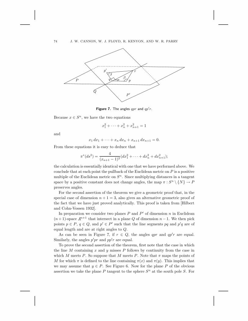
In preparation we consider two planes P and P ′ of dimension n in Euclidean
(n+ 1)-space� n+1 that intersect in a plane Q of dimension n− 1. We then pick
points p ∈ P , q ∈ Q, and p′ ∈ P ′ such that the line segments pq and p′q are of
equal length and are at right angles to Q.
As can be seen in Figure 7, if r ∈ Q, the angles qpr and qp′r are equal.
Similarly, the angles p′pr and pp′r are equal.
To prove the second assertion of the theorem, first note that the case in which
the line M containing x and y misses P follows by continuity from the case in
which M meets P . So suppose that M meets P . Note that π maps the points of
M for which π is defined to the line containing π(x) and π(y). This implies that
we may assume that y ∈ P . See Figure 6. Now for the plane P of the obvious
assertion we take the plane P tangent to the sphere Sn at the south pole S. For

HYPERBOLIC GEOMETRY 75
the plane P ′ of the obvious assertion we take the plane tangent to Sn at x. For
the points p′ ∈ P ′ and p ∈ P we take, respectively, the points p = π(x) ∈ P and
p′ = x ∈ P ′. For the plane Q we take the intersection of P and P ′. For the point
r we take y. Now the assertion that the angles p′pr and pp′r are equal proves
the second assertion of the theorem.
In dimension three, the obvious fact that the angles qpr and qp′r are equal
shows that π preserves the angle between any given curve and certain reference
tangent directions, namely pq and p′q. Since the tangent space is, in this dimen-
sion only, two-dimensional, preserving angle with reference tangent directions is
enough to ensure preservation of angle in general. �
Theorem 8.2 (Preservation of spheres). Assume the setting of the previous
theorem. If C is a sphere (C for circle) in Sn that passes through the north pole
N of Sn and has dimension c, then the image π(C) ⊂ P is a plane in P of
dimension c. If on the other hand C misses N , then the image π(C) is a sphere
in P of dimension c.
Proof. If N ∈ C, then the proof is easy; indeed C is contained in a unique
plane P ′ of dimension c+1, and the image π(C) is the intersection of P ′ and P ,
a c-dimensional plane.
If, on the other hand, C misses N , we argue as follows. We assume all
normalized as in the analytic portion of the proof of the previous theorem so
that Sn is the unit sphere. We can deal with the case where C is a union of
great circles by continuity if we manage to prove the theorem in all other cases.
Consequently, we may assume that the vector subspace of� n+1 spanned by the
vectors in C has dimension c + 2. We lose no generality in assuming that it is
all of� n+1 (that is, c = n− 1).
The tangent spaces to Sn at the points of C define a conical envelope with
cone point y; one easy way to find y is to consider the two-dimensional plane R
containing N and two antipodal points r and r′ of C, and to consider the two
tangent lines t(r) to C ∩ R at r and t(r′) to C ∩ R at r′; then y is the point at
which t(r) and t(r′) meet. See Figure 8. By continuity we may assume that π(y)
is defined.
We assert that π(y) is equidistant from the points of π(C), from which the
reader may deduce that π(C) is a sphere centered at π(y). By continuity it
suffices to prove that π(y) is equidistant from the points of π(C) \ S. Here
is the argument that proves the assertion. Let x ∈ C \ S, and consider the
two-dimensional plane containing N , x, and y. In this plane there is a point
x′ on the line through x and N such that the line segment yx′ is parallel to
the segment π(y)π(x); that is, the angles N π(x)π(y) and N x′ y are equal. By
the final assertion of Theorem 8.1, the angles π(y)π(x)x and y x π(x) are either
equal or complementary. Thus the triangle xyx′ is isosceles so that sides xy and
x′y are equal. Thus considering proportions in the similar triangles N x′ y and

76 J. W. CANNON, W. J. FLOYD, R. KENYON, AND W. R. PARRY
•
•
•
←
←
N
C
Sn
y
P
π(C)
π(y)
Figure 8. Stereographic projection maps spheres to spheres.
N π(x)π(y), we have the equalities
d(π(x), π(y)) =d(N, π(y))
d(N, y)d(x′, y) =
d(N, π(y))
d(N, y)d(x, y).
Of course, the fraction is a constant since N , y, and π(y) do not depend on x;
and the distance d(x, y) is also a constant since x ∈ C, C is a sphere, and y is
the center of the tangent cone of C. We conclude that the distance d(π(x), π(y))
is constant. �
Definition. Let Sn denote a sphere of dimension n in� n+1 with north pole N
and south pole S as above. Let P denote a plane through the center of Sn and
orthogonal to the line through N and S. If x is any point of Sn\{N}, then there
is a unique point π′(x) of P on the line that contains N and x. This defines a
map π′ : Sn \ {N} → P , stereographic projection from Sn \ {N} to P .
Theorem 8.3. The map π′ preserves angles between curves in Sn \ {N}, and
π′ maps spheres to planes or spheres .
Proof. We normalize so that Sn is the unit sphere in� n+1 , N = (0, . . . , 0, 1),
and S = (0, . . . , 0,−1). From the proof of Theorem 8.1 we have for every x ∈Sn \ {N} that π(x) = (y1, . . . , yn,−1), where
yi =−2
xn+1 − 1xi.
In the same way π′(x) = (y′1, . . . , y′n,−1), where
y′i =−1
xn+1 − 1xi =
yi
2.
Thus π′ is the composition of π with a translation and a dilation. Since π
preserves angles and maps spheres to planes or spheres, so does π′. �
HYPERBOLIC GEOMETRY 77
•
•
r
r
r
r
r(pa
th)
path
geodesic
r = distance-reducing retraction
r(path) is shorter than path
Figure 9. The retraction principle.
9. Geodesics
Having established formulas for the hyperbolic metric in our five analytic
models and having developed the fundamental properties of stereographic pro-
jection, it is possible to find the straight lines or geodesics in our five models
with a minimal amount of effort. Though geodesics can be found by solving
differential equations, we shall not do so. Rather, we establish the existence of
one geodesic in the half-space model by means of what we call the retraction
principle. Then we deduce the nature of all other geodesics by means of simple
symmetry properties of the hyperbolic metrics. Here are the details. We learned
this argument from Bill Thurston.
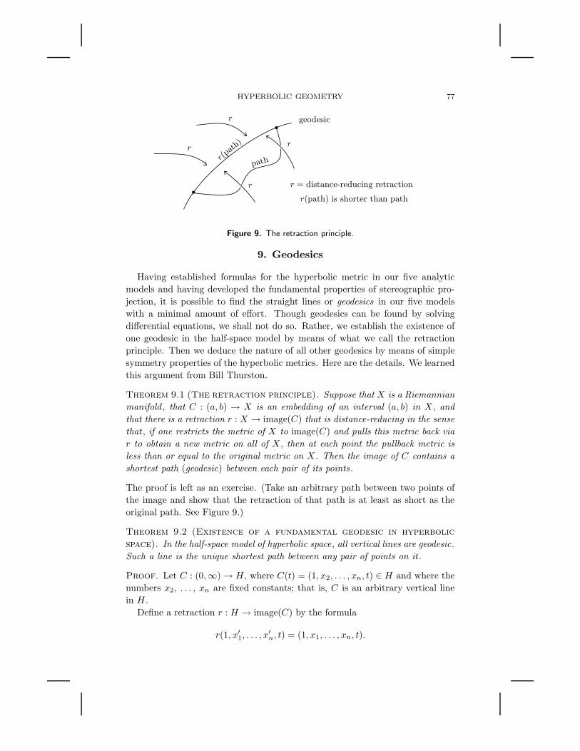
Theorem 9.1 (The retraction principle). Suppose that X is a Riemannian
manifold , that C : (a, b) → X is an embedding of an interval (a, b) in X , and
that there is a retraction r : X → image(C) that is distance-reducing in the sense
that , if one restricts the metric of X to image(C) and pulls this metric back via
r to obtain a new metric on all of X , then at each point the pullback metric is
less than or equal to the original metric on X . Then the image of C contains a
shortest path (geodesic) between each pair of its points .
The proof is left as an exercise. (Take an arbitrary path between two points of
the image and show that the retraction of that path is at least as short as the
original path. See Figure 9.)
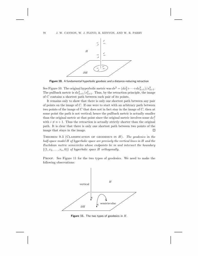
Theorem 9.2 (Existence of a fundamental geodesic in hyperbolic
space). In the half-space model of hyperbolic space, all vertical lines are geodesic.
Such a line is the unique shortest path between any pair of points on it .
Proof. Let C : (0,∞) → H , where C(t) = (1, x2, . . . , xn, t) ∈ H and where the
numbers x2, . . . , xn are fixed constants; that is, C is an arbitrary vertical line
in H .
Define a retraction r : H → image(C) by the formula
r(1, x′1, . . . , x′n, t) = (1, x1, . . . , xn, t).
78 J. W. CANNON, W. J. FLOYD, R. KENYON, AND W. R. PARRY
↑↑
↑↑
↑↑
←
←
←
←
←
←
H
∂H
Figure 10. A fundamental hyperbolic geodesic and a distance-reducing retraction
See Figure 10. The original hyperbolic metric was ds2 = (dx22+· · ·+dx2
n+1)/x2n+1.
The pullback metric is dx2n+1/x
2n+1. Thus, by the retraction principle, the image
of C contains a shortest path between each pair of its points.
It remains only to show that there is only one shortest path between any pair
of points on the image of C. If one were to start with an arbitrary path between
two points of the image of C that does not in fact stay in the image of C, then at
some point the path is not vertical; hence the pullback metric is actually smaller
than the original metric at that point since the original metric involves some dx2i
with i 6= n+ 1. Thus the retraction is actually strictly shorter than the original
path. It is clear that there is only one shortest path between two points of the
image that stays in the image. �
Theorem 9.3 (Classification of geodesics in H). The geodesics in the
half-space model H of hyperbolic space are precisely the vertical lines in H and the
Euclidean metric semicircles whose endpoints lie in and intersect the boundary
{(1, x2, . . . , xn, 0)} of hyperbolic space H orthogonally .
Proof. See Figure 11 for the two types of geodesics. We need to make the
following observations:
•
• •
H
∂H
vertical
semicircular
Figure 11. The two types of geodesics in H.
HYPERBOLIC GEOMETRY 79
•••
••
p
q
p′ q′r
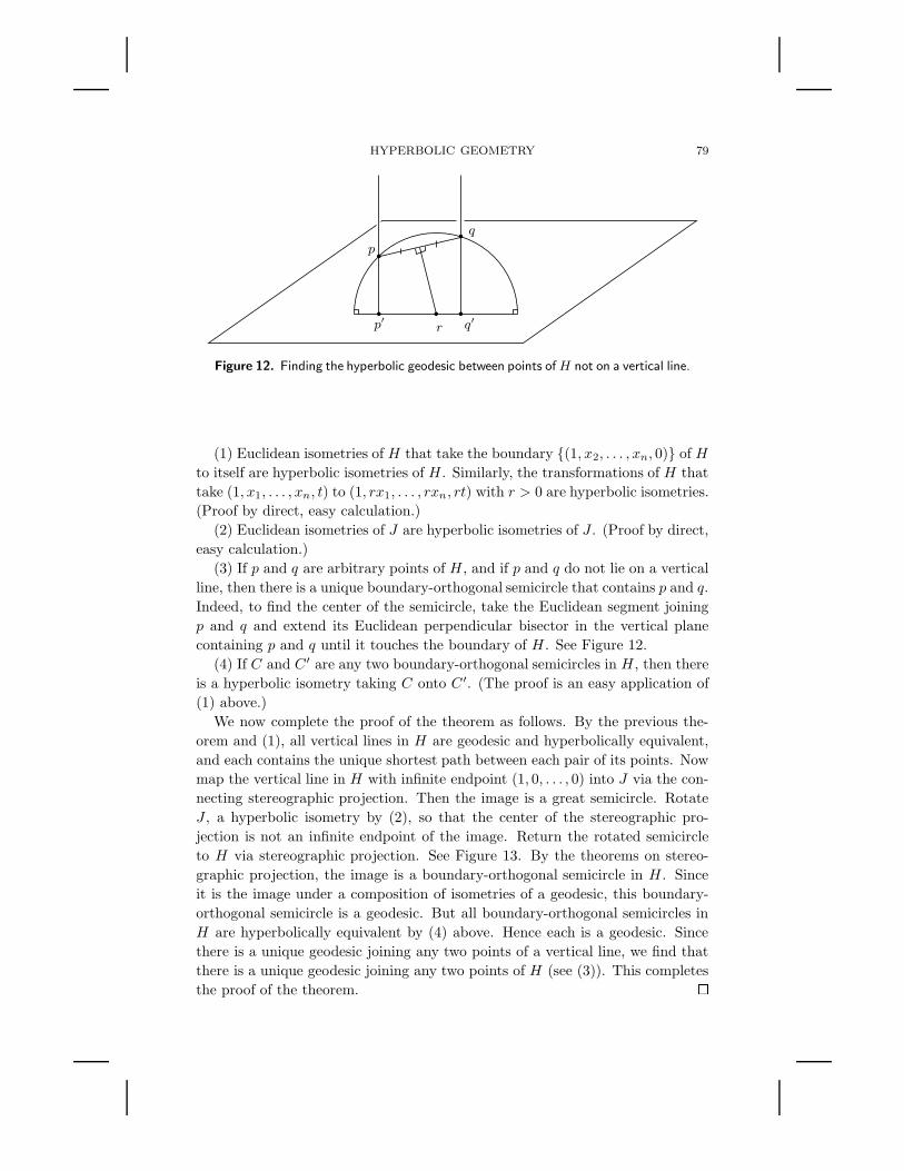
Figure 12. Finding the hyperbolic geodesic between points ofH not on a vertical line.
(1) Euclidean isometries of H that take the boundary {(1, x2, . . . , xn, 0)} of H
to itself are hyperbolic isometries of H . Similarly, the transformations of H that
take (1, x1, . . . , xn, t) to (1, rx1, . . . , rxn, rt) with r > 0 are hyperbolic isometries.
(Proof by direct, easy calculation.)
(2) Euclidean isometries of J are hyperbolic isometries of J . (Proof by direct,
easy calculation.)
(3) If p and q are arbitrary points of H , and if p and q do not lie on a vertical
line, then there is a unique boundary-orthogonal semicircle that contains p and q.
Indeed, to find the center of the semicircle, take the Euclidean segment joining
p and q and extend its Euclidean perpendicular bisector in the vertical plane
containing p and q until it touches the boundary of H . See Figure 12.
(4) If C and C ′ are any two boundary-orthogonal semicircles in H , then there
is a hyperbolic isometry taking C onto C ′. (The proof is an easy application of
(1) above.)
We now complete the proof of the theorem as follows. By the previous the-
orem and (1), all vertical lines in H are geodesic and hyperbolically equivalent,
and each contains the unique shortest path between each pair of its points. Now
map the vertical line in H with infinite endpoint (1, 0, . . . , 0) into J via the con-
necting stereographic projection. Then the image is a great semicircle. Rotate
J , a hyperbolic isometry by (2), so that the center of the stereographic pro-
jection is not an infinite endpoint of the image. Return the rotated semicircle
to H via stereographic projection. See Figure 13. By the theorems on stereo-
graphic projection, the image is a boundary-orthogonal semicircle in H . Since
it is the image under a composition of isometries of a geodesic, this boundary-
orthogonal semicircle is a geodesic. But all boundary-orthogonal semicircles in
H are hyperbolically equivalent by (4) above. Hence each is a geodesic. Since
there is a unique geodesic joining any two points of a vertical line, we find that
there is a unique geodesic joining any two points of H (see (3)). This completes
the proof of the theorem. �

80 J. W. CANNON, W. J. FLOYD, R. KENYON, AND W. R. PARRY
•
•
•
•
•
•
H
J
M ′
M ′ = semicircular rotate of α−1(M)
vertical geodesic M
α(M ′) = semicircularimage of M ′
semicircle α−1(M)
Figure 13. Geodesics in H.
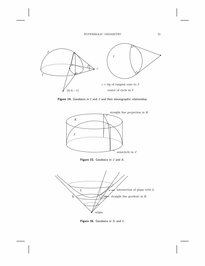
By Theorems 8.1 and 8.2, the boundary-orthogonal semicircles in J correspond
precisely to the boundary-orthogonal semicircles and vertical lines in H . Hence
the geodesics in J are the boundary-orthogonal semicircles in J .
By Theorem 8.3, the boundary-orthogonal semicircles in J correspond to the
diameters and boundary-orthogonal circular segments in I . Hence the diameters
and boundary-orthogonal circular segments in I are the geodesics in I . See
Figure 14.
The boundary-orthogonal semicircles in J clearly correspond under vertical
projection to straight line segments in K. Hence the latter are the geodesics in
K. See Figure 15.
The straight line segments in K clearly correspond under central projection
from the origin to the intersections with L of two-dimensional vector subspaces
of� n+1 with L; hence the latter are the geodesics of L. See Figure 16.
10. Isometries and Distances in the Hyperboloid Model
We begin our study of the isometries of hyperbolic space with the hyperboloid
model L where all isometries, as we shall see, are restrictions of linear maps of� n+1 .
Definition. A linear isometry f : L→ L of L is the restriction to L of a linear
map F :� n+1 → � n+1 that preserves the hyperbolic inner product ∗ (that is,
HYPERBOLIC GEOMETRY 81
•
•
•
••
I
I
J
c
(0, 0,−1)
c = tip of tangent cone to J
center of circle in I
Figure 14. Geodesics in I and J and their stereographic relationship.
↑↑
J
K
straight line projection in K
semicircle in J
Figure 15. Geodesics in J and K.
•
←←
straight line geodesic in K
origin
K
L intersection of plane with L
Figure 16. Geodesics in K and L.

82 J. W. CANNON, W. J. FLOYD, R. KENYON, AND W. R. PARRY
for each pair v and w of vectors from� n+1 , Fv ∗ Fw = v ∗ w) and that takes
the upper sheet of the hyperboloid L into itself.
Definition. A Riemannian isometry f : L → L of L is a diffeomorphism of L
that preserves the Riemannian metric (that is, f ∗(ds2) = ds2).
Definition. A topological isometry f : L → L of L is a homeomorphism of L
that preserves the Riemannian distance between each pair of points of L (that
is, if d is the Riemannian distance function and if x and y are points of L, then
d(f(x), f(y)) = d(x, y)).
Theorem 10.1. A square matrix M with columns m1, . . . , mn, mn+1 induces
a linear isometry of L if and only if the following two conditions are satisfied .
1. For each pair of indices i and j, we have mi ∗mj = ei ∗ ej , where e1, . . . , en,
en+1 is the standard basis for� n+1 .
2. The last entry of the last column mn+1 is positive.
Condition 1 is satisfied if and only if M is invertible with M−1 = JM tJ , where
J is the diagonal matrix with diagonal entries J11 = · · · = Jnn = −Jn+1,n+1 = 1.
Proof. Let J denote the diagonal matrix with diagonal entries J11 = · · · =
Jnn = −Jn+1,n+1 = 1. Then for each x, y ∈ � n+1 , x∗y = xtJy. ThusMx∗My =
xtM tJMy. Consequently, M preserves ∗ if and only if M tJM = J ; but the ij
entry of M tJM is mi ∗mj while that of J is ei ∗ ej . Thus M preserves ∗ if and
only if condition 1 of the theorem is satisfied. Since J is invertible, condition 1
implies that M is also invertible and that it takes the hyperboloid of two sheets,
of which L is the upper sheet, homeomorphically onto itself. Condition 2 is then
just the statement that the image of en+1 lies in L, that is, that M takes the
upper sheet L of the hyperboloid onto itself.
Finally, the equality M−1 = JM tJ is clearly equivalent to the equality
M tJM = J since J−1 = J . �
Theorem 10.2. A map f : L → L that satisfies any of the three definitions of
isometry—linear , Riemannian, or topological—satisfies the other two as well .
Proof. We first prove the two easy implications, linear ⇒ Riemannian ⇒topological, then connect the hyperbolic inner product x ∗ y with Riemannian
distance d(x, y) in preparation for the more difficult implication, topological ⇒linear.
Linear isometry ⇒ Riemannian isometry: Let F :� n+1 → � n+1 be a linear
map that preserves the hyperbolic inner product ∗ and takes the upper sheet L
of the hyperboloid of two sheets into itself and thereby induces a linear isometry
f : L→ L. The Riemannian metric ds2 is at each point x of L simply a function
of two variables that takes as input two tangent vectors v and w at x and delivers
as output the hyperbolic inner product v ∗ w. We calculate the pullback metric

HYPERBOLIC GEOMETRY 83
f∗(ds2) in the following manner:
f∗(ds2)(v, w) = ds2(Df(v), Df(w)) = ds2(DF (v), DF (w))
= ds2(F (v), F (w)) = F (v) ∗ F (w) = v ∗ w = ds2(v, w).
We conclude that f∗(ds2) = ds2, so that f is a Riemannian isometry.
Riemannian isometry ⇒ topological isometry: Riemannian distance is calculated
by integrating the Riemannian metric. Since a Riemannian isometry preserves
the integrand, it preserves the integral as well.
Lemma. If a, b ∈ L, then a ∗ b = − cosh(d(a, b)).
Proof. Let t denote the Riemannian distance d(a, b) between a and b. One
obtains this distance by integrating the Riemannian metric along the unique
geodesic path joining a and b, or, since this integral is invariant under linear
isometry, one can translate a and b to a standard position in L as follows and
then perform the integration. Let m1 be the unit tangent vector at a in the
direction of the geodesic from a to b. Let mn+1 = a. By the Gram–Schmidt
orthonormalization process from elementary linear algebra we may extend the
orthonormal set {m1,mn+1} to an orthonormal basis m1, . . . , mn, mn+1 for� n+1 ; that is, mi ∗mj = ei ∗ ej . By Theorem 10.1, the matrix M with columns
m1, . . . , mn, mn+1 gives a linear isometry of L as does its inverse M−1. The
inverse takes a to en+1 and takes the two-dimensional subspace spanned by a
and b to the space P spanned by e1 and en+1. The intersection of P with L is one
branch of a standard hyperbola that passes through M−1(a) and M−1(b) and
is the unique hyperbolic geodesic through those two points. Since M−1(a) =
(0, . . . , 0, 1) and since t = d(a, b) = d(M−1(a),M−1(b)), we may assume that
M−1(b) = (sinh(t), . . . , 0, cosh(t)). (See Section 4.) Thus we may calculate:
a ∗ b = M−1(a) ∗M−1(b) = (0, . . . , 0, 1) ∗ (sinh(t), . . . , 0, cosh(t))
= − cosh(t) = − cosh(d(a, b)). �
Topological isometry ⇒ linear isometry: Let f : L → L denote a topological
isometry. Let v1, . . . , vn, vn+1 denote a basis for� n+1 such that each vi lies in
L. Let F denote the linear map that takes vi to f(vi) for each i. We claim that
F preserves ∗; to see this, write ei =∑
j aijvj and compute:
F (ei) ∗ F (ej) =∑
k,l
aikajlf(vk) ∗ f(vl)
=∑
k,l
aikajl(− cosh(d(f(vk), f(vl))))
=∑
k,l
aikajl(− cosh(d(vk , vl))) = ei ∗ ej .
Moreover, F agrees with f on L. To prove this, it suffices to replace f by F−1◦f ,
so that we can assume f(vi) = vi; then we must prove that f = id, which we
84 J. W. CANNON, W. J. FLOYD, R. KENYON, AND W. R. PARRY
can do by showing f(x) ∗ ei = x ∗ ei for each x ∈ L and for each index i. Here is
the calculation:
f(x) ∗ ei = f(x) ∗∑
j
aijvj =∑
j
aij(f(x) ∗ f(vj))
=∑
j
aij(− cosh(d(f(x), f(vj))))
=∑
j
aij(− cosh(d(x, vj))) = x ∗ ei. �
11. The Space at Infinity
It is apparent from all of our analytic models with the possible exception of
the hyperboloid model L that there is a natural space at infinity. In the half-
space model H it is the bounding plane of dimension n− 1 that we compactify
by adding one additional point; we visualize the additional point as residing at
the top of the collection of vertical geodesics in H . In the disk model I , in the
hemisphere model J , and in the Klein model K it is the bounding (n−1)-sphere.
If we reinterpret the hyperboloid model as lying in projective space (each point
of L is represented by the unique one-dimensional vector subspace of� n+1 that
contains that point), then the space at infinity becomes apparent in that model
as well: it consists of those lines that lie in the light cone {x ∈ � n+1 : x∗x = 0}.Furthermore, it is apparent that not only the models but also the unions of
those models with their spaces at infinity correspond homeomorphically under
our transformations connecting the models. That is, the space at infinity is a
sphere of dimension n− 1 and the union of the model with the space at infinity
is a ball of dimension n.
Having analyzed the isometries of the hyperboloid model, we see that each
isometry of L actually extends naturally not only to the space at infinity but to
the entirety of projective n-space. That is, each linear mapping of� n+1 defines
a continuous mapping of projective n-space P n.
12. The Geometric Classification of Isometries
We recall from the previous sections that every isometry f of L extends to a
linear homeomorphism F of� n+1 , hence upon passage to projective space P n
induces a homeomorphism f ∪f∞ : L∪∂L→ L∪∂L of the ball that is the union
of hyperbolic space L and its space ∂L at infinity. Every continuous map from
a ball to itself has a fixed point by the Brouwer fixed point theorem. There is a
very useful and beautiful geometric classification of the isometries of hyperbolic
space that refers to the fixed points of this extended map. Our analysis of these
maps requires that we be able to normalize them to some extent by moving given
fixed points into a standard position. To that end we note that we have already
shown how to move any point in L and nonzero tangent vector at that point
HYPERBOLIC GEOMETRY 85
so that the point is at en+1 and the tangent points in the direction of e1. As a
consequence we can move any pair of points in L ∪ ∂L so that they lie in any
given geodesic; and by conjugation we find that we may assume that any pair of
fixed points of an isometry lies in a given geodesic. Indeed, let f be an isometry
with fixed point x, let g be an isometry that takes x into a geodesic line L, and
note that g(x) is a fixed point of gfg−1. Here are the three possible cases.
The elliptic case occurs when the extended map has a fixed point in L itself:
conjugating by a linear isometry of L, we may assume that the isometry f :
L → L fixes the point en+1 = (0, . . . , 0, 1). Let F :� n+1 → � n+1 be the linear
extension of f . The representing matrix M has as last column mn+1 the vector
en+1. The remaining columns must be ∗-orthogonal to mn+1, hence Euclidean
or ·-orthogonal to en+1. On the orthogonal complement of en+1, the hyperbolic
and the Euclidean inner products coincide. Hence the remaining columns form
not only a hyperbolic orthonormal basis but also a Euclidean orthonormal basis.
We conclude that the matrix M defining F is actually Euclidean orthogonal. We
call such a transformation of hyperbolic space elliptic.
The hyperbolic case occurs when the extended map has no fixed point in L itself
but has two fixed points at infinity: we examine this transformation in the half-
space model H for hyperbolic space. We ignore the initial constant coordinate
1 in H and identify H with the half-space {x = (x1, . . . , xn) ∈ � n : xn > 0}.Conjugating by an isometry, we may assume that the fixed points of the map f
of H ∪ ∂H are the infinite endpoints of the hyperbolic geodesic (0, . . . , t), where
t > 0. Let (0, . . . , k) denote the image under f of (0, . . . , 1). Then (1/k) · f is
an isometry that fixes every point of the hyperbolic geodesic (0, . . . , t). By the
previous paragraph, the transformation (1/k) ·f is an orthogonal transformation
O. It follows easily that f(x) = k O(x), the composite of a Euclidean orthogonal
transformation O, which preserves the boundary plane at infinity and which
is simultaneously a hyperbolic isometry, with the hyperbolic translation x 7→kx along the geodesic (0, . . . , t). Such a transformation is called hyperbolic or
loxodromic. The invariant geodesic (0, . . . , t) is called the axis of the hyperbolic
transformation. See Figure 17. Often one preserves the name hyperbolic for the
case where the orthogonal transformation is trivial and the name loxodromic for
the case where the orthogonal transformation is nontrivial.
The parabolic case occurs when the extended map has only one fixed point and
that fixed point is at infinity: we examine this transformation in the half-space
model H for hyperbolic space. We may assume that the fixed point of the map
f of H ∪ ∂H is the upper infinite endpoint of the hyperbolic geodesic (0, . . . , t),
where t > 0. The transformation g : x 7→ f(x) − f((0, . . . , 0)) fixes both ends
of the same geodesic. Hence g may be written as a composite x 7→ k O(x)
where k > 0 and O have the significance described in the previous paragraph.
Thus f(x) = k O(x) + v, where k > 0, O is Euclidean orthogonal preserving the
boundary plane of H , and v = f((0, . . . , 0)) is a constant vector. We claim that
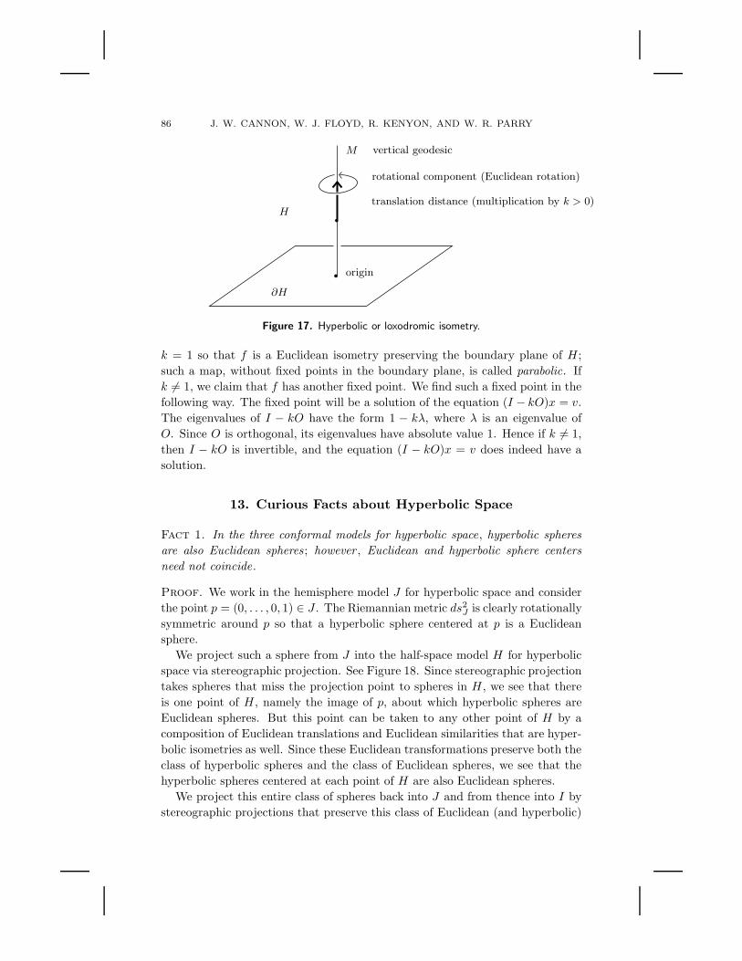
86 J. W. CANNON, W. J. FLOYD, R. KENYON, AND W. R. PARRY
•
•H
∂H
origin
M vertical geodesic
rotational component (Euclidean rotation)
translation distance (multiplication by k > 0)
Figure 17. Hyperbolic or loxodromic isometry.
k = 1 so that f is a Euclidean isometry preserving the boundary plane of H ;
such a map, without fixed points in the boundary plane, is called parabolic. If
k 6= 1, we claim that f has another fixed point. We find such a fixed point in the
following way. The fixed point will be a solution of the equation (I − kO)x = v.
The eigenvalues of I − kO have the form 1 − kλ, where λ is an eigenvalue of
O. Since O is orthogonal, its eigenvalues have absolute value 1. Hence if k 6= 1,
then I − kO is invertible, and the equation (I − kO)x = v does indeed have a
solution.
13. Curious Facts about Hyperbolic Space
Fact 1. In the three conformal models for hyperbolic space, hyperbolic spheres
are also Euclidean spheres ; however , Euclidean and hyperbolic sphere centers
need not coincide.
Proof. We work in the hemisphere model J for hyperbolic space and consider
the point p = (0, . . . , 0, 1) ∈ J . The Riemannian metric ds2J is clearly rotationally
symmetric around p so that a hyperbolic sphere centered at p is a Euclidean
sphere.
We project such a sphere from J into the half-space model H for hyperbolic
space via stereographic projection. See Figure 18. Since stereographic projection
takes spheres that miss the projection point to spheres in H , we see that there
is one point of H , namely the image of p, about which hyperbolic spheres are
Euclidean spheres. But this point can be taken to any other point of H by a
composition of Euclidean translations and Euclidean similarities that are hyper-
bolic isometries as well. Since these Euclidean transformations preserve both the
class of hyperbolic spheres and the class of Euclidean spheres, we see that the
hyperbolic spheres centered at each point of H are also Euclidean spheres.
We project this entire class of spheres back into J and from thence into I by
stereographic projections that preserve this class of Euclidean (and hyperbolic)

HYPERBOLIC GEOMETRY 87
•
•
H
∂HJ
π(C)
π(p)
pC
Figure 18. The projection of a sphere from J to H. C is both a Euclidean and
a hyperbolic sphere; π(p) is the hyperbolic center of the circle π(C).
spheres. We conclude that all hyperbolic spheres in these three models are also
Euclidean spheres, and conversely.
Finally, we give a geometric construction for the hyperbolic center of a Eu-
clidean sphere S in the half-space model H . See Figure 19. Draw the vertical
geodesic line M through the center of S until it meets the plane at infinity at
some point p. Draw a tangent line to S from p meeting S at a tangency point
q. Draw the circle C through q that is centered at p and lies in the same plane
as M . The circle C then meets the line M at the hyperbolic center of S (proof,
an exercise for the reader). Note that this center is not the Euclidean center
of S. �
←
•
• ←←•
H
M
hyperbolic centerEuclidean centerhyperbolic diameter
∂H
Figure 19. Constructing the hyperbolic center of a circle

88 J. W. CANNON, W. J. FLOYD, R. KENYON, AND W. R. PARRY
•
•←
•
HC
pr
∂H
envelope = equidistant curve
hyperbolic equidistant curveis Euclidean straight line
M= vertical geodesic line
Figure 20. Equidistant curves in H.
Fact 2. In the hyperbolic plane, the two curves at distance r on either side of
a straight line are not straight .
Proof. We can use the preceding result to analyze the curves equidistant from
a hyperbolic geodesic in the hyperbolic plane. We work in the half-space model
H ⊂ � 2 of the two-dimensional hyperbolic plane and take as geodesic line the
vertical line M that passes through the origin of� 2 . Put a hyperbolic circle C
of hyperbolic radius r about a point p of M . Then we obtain the set of all such
circles centered at points of M by multiplying C by all possible positive scalars.
The union of these spheres t · C is a cone, or angle, D of which the origin is the
vertex and whose central axis is M . The envelope or boundary of this cone or
angle is a pair of Euclidean straight lines, the very equidistant lines in which we
are interested. See Figure 20. Since these straight lines are not vertical, they are
not hyperbolic straight lines. �
Fact 3. Triangles in hyperbolic space have angle sum less than π; in fact , the
area of a triangle with angles α, β, and γ is π − α − β − γ (the Gauss–Bonnet
theorem). Given three angles α, β, and γ whose sum is less than π, there is one
and only one triangle up to congruence having those angles . Consequently , there
are no nontrivial similarities of hyperbolic space.
Proof. Any triangle in hyperbolic space lies in a two-dimensional hyperbolic
plane. Hence we may work in the half-space model H for the hyperbolic plane.
Assume that we are given a triangle ∆ = pqr with angles α, β, and γ. We may
arrange via an isometry of hyperbolic space that the side pq lies in the unit circle.
Then by a hyperbolic isometry of hyperbolic space that has the unit circle as its
invariant axis and translates along the unit circle we may arrange that the side
pr points vertically upward. The resulting picture is in Figure 21.

HYPERBOLIC GEOMETRY 89
•
••
•
π − γ
∞∞
γ
βα
α
β′
β + β′
∂H
H
q
r
p
Figure 21. The Gauss–Bonnet theorem.
We note that the triangle ∆ = pqr is the difference of two ideal triangles pq∞and rq∞. (“Ideal” means that at least one vertex is at infinity.) We first prove
the Gauss–Bonnet theorem for such an ideal triangle, then deduce the desired
formula by taking a difference.
The element of area is dA = dx dy/y2. It is easy to verify that the area of
pq∞ is therefore
∫
pq∞dA =
∫ x=cos(π−α)
x=cos(β+β′)
dx
∫ y=∞
y=√
1−x2
dy
y2.
Straightforward evaluation leads to the value π − α − β − β ′ for the integral.
Similar evaluation gives the value π − (π − γ) − β′ for the area of rq∞. The
difference of these two values is π − α − β − γ as claimed. This proves the
Gauss–Bonnet theorem.
We now construct a triangle with given angles. Suppose therefore that three
angles α, β, and γ are given whose sum is less than π, a necessary restriction in
view of the Gauss–Bonnet theorem. Pick a model of the hyperbolic plane, say
the disk model I . Pick a pair Q and R of geodesic rays (radii) from the origin p
meeting at the Euclidean (= hyperbolic) angle of α. See Figure 22. Note that
any pair of geodesic rays meeting at angle α is congruent to this pair. Pick points
q and r on these rays and consider the triangle pqr. Let β ′ denote the angle at q
and let γ′ denote the angle at r. Let A′ denote the area of the triangle pqr. We
will complete the construction by showing that there is a unique choice for q on
Q and for r on R such that β′ = β and γ′ = γ. The argument will be variational.
We first consider the effect of fixing a value of q and letting r vary from ∞to p along R. At ∞, the angle γ ′ is 0. At (near) p the angle γ ′ is (almost)
π − α. As r moves inward toward p along R, both β′ and A′ clearly decrease
monotonically. Hence, by the Gauss–Bonnet theorem, γ ′ = π − α − β′ − A′
increases monotonically. In particular, there is a unique point r(q) at which

90 J. W. CANNON, W. J. FLOYD, R. KENYON, AND W. R. PARRY
•
•
•
p = origin
q
rQ R
∞
∞
α
β′
γ′
Figure 22. Constructing a triangle with angles α, β, and γ, with α+ β+ γ < π
γ′ = γ. Now fix q, fix r at r(q), and move inward along Q from q to a point q′.
Note that the angle of pq′r at r is smaller than the angle γ, which is the angle
of pqr at r. We conclude that r(q′) must be closer to p than is r(q). That is, as
q moves inward toward p, so also does r(q). We conclude that the areas of the
triangles pqr(q) decrease monotonically as q moves inward along Q toward p.
We are ready for the final variational argument. We work with the triangles
pqr(q). We start with q at ∞ and note that the area A′ is equal to π−α−0−γ >π − α− β − γ. We move q inward along Q, and consequently move r(q) inward
along R, until q reaches p and A′ = 0 < π−α−β− γ. As noted in the previous
paragraph, the area A′ decreases monotonically. Hence there is a unique value
of q at which the area is π − α − β − γ. At that value of q the angle β ′ must
equal β by the Gauss–Bonnet theorem. �
Fact 4. If ∆ = pqr is a triangle in hyperbolic space, and if x is a point of the
side pq, then there is a point y ∈ pr∪ qr such that the hyperbolic distance d(x, y)
is less than ln(1 +√
2); that is , triangles in hyperbolic space are uniformly thin.
Proof. We need two observations. First, if P and Q are two vertical geodesics
in the half-space model H for hyperbolic space, and if a point p moves monoton-
ically downward along P , then the distance d(p,Q) increases monotonically to
infinity. See Figure 23. Second, if p and q are two points on the same boundary-
orthogonal semicircle (geodesic) in H , say on the unit circle with coordinates
p = (cos(φ), sin(φ)) and q = (cos(θ), sin(θ)) with θ > φ, then the hyperbolic
distance between the two is given by the formula
d(p, q) =
∫ θ
φ
dψ
sin(ψ)= ln
sin(ψ)
1 + cos(ψ)
∣
∣
∣
∣
θ
φ
.
See Figure 24. Actually, the radius of the semicircle is irrelevant because scaling
is a hyperbolic isometry. Only the beginning and ending angles are important.
We are now ready for the proof that triangles are thin. Let ∆ = pqr denote
a triangle in the hyperbolic plane. We view ∆ in the half-space model of the

HYPERBOLIC GEOMETRY 91
�
←d(p,Q)
d(p,Q)
d(p,Q)
p
PQ
H
∂H
hyperbolic equidistant curve
Figure 23. The monotonicity of d(p,Q).
hyperbolic plane. We may assume that the side pq lies in the unit circle with p to
the left of q, and we may assume that the side pr is vertical with r above p. We
assume a point x ∈ pq given. See Figure 25. We want to find an upper bound for
the distance d(x, pr ∪ qr). The following operations simply expand the triangle
∆ and hence increase the distance that we want to bound above. First we may
move r upward until it moves to ∞. We may then slide p leftward along the unit
circle until it meets infinity at p′ = −1. We may then slide q rightward along the
unit circle until it meets infinity at q′ = 1. We now have an ideal triangle p′q′∞with x ∈ p′q′. See Figure 26. The pair of sides p′q′ and p′∞ are congruent as a
pair to a pair of vertical geodesics (simply move p′ to ∞ by an isometry of H).
Hence as we move x toward q′, the distance d(x, p′∞) increases monotonically.
Similarly, as we move x toward p′, the distance d(x, q′∞) increases monotonically.
We conclude that the maximum distance to p′∞∪ q′∞ is realized when x is at
the topmost point of the unit circle. The distances to the two vertical geodesics
p′∞ and q′∞ are then equal and the shortest path is realized by a boundary-
orthogonal semicircle that passes through x and meets, say, p′∞ orthogonally (if
it did not meet orthogonally, then a shortcut near the vertical geodesic would
reduce the length of the path). It is clear from the geometry that this shortest
•
•••
• geodesic
geodesic
p
p′q
q′
φπ − θ
d(p, q) = d(p′, q′) =
�geodesic
ds =
� θ
φ
dψ
sinψ
Figure 24. The formula for d(p, q).

92 J. W. CANNON, W. J. FLOYD, R. KENYON, AND W. R. PARRY
••
•
•
xq
q′
p
p′
r
∞ = r′ ∞ = r′
∂H
H
••
π/4
x′x
q′
Q′
p′
P ′
∞ = r′ ∞ = r′
∂H
H
Figure 25. Triangles are thin. Figure 26. The ideal triangle p′q′∞.
path travels through the angle interval [π/4, π/2] in going from x to the vertical
geodesic p′∞. Hence, by our calculation above, the distance between the point
and the opposite sides is
lnsin(π/2)
1 + cos(π/2)− ln
sin(π/4)
1 + cos(π/4)= ln
(
1 +√
2)
= 0.88 . . . .
We conclude that triangles are uniformly thin, as claimed. �
Fact 5. For a circular disk in the hyperbolic plane, the ratio of area to cir-
cumference is less than 1 and approaches 1 as the radius approaches infinity .
That is , almost the entire area of the disk lies very close to the circular edge of
the disk . Both area and circumference are exponential functions of hyperbolic
radius .
Proof. We do our calculations in the disk model I of the hyperbolic plane.
The Riemannian metric is, as we recall,
ds2I = 4(dx21 + · · · + dx2
n)/(1 − x21 − · · ·x2
n)2.
We are considering the case n = 2. Using polar coordinates (see Section 6) we
can easily compute the distance element along a radial arc, namely
ds = 2dr
1 − r2,
while the area element is
dA =4
(1 − r2)2r dr dθ.
We fix a Euclidean radius R with associated circular disk centered at the origin
in I and calculate the hyperbolic radius ρ, area A, and circumference C (see

HYPERBOLIC GEOMETRY 93
••
I
C
A
ρ
(1, 0)(R, 0)
Figure 27. The hyperbolic radius ρ, the area A, and the circumference C.
Figure 27):
ρ =
∫ R
0
2dr
1 − r2= ln
1 +R
1 −R;
A =
∫ 2π
θ=0
∫ R
r=0
4
(1 − r2)2r dr dθ =
4πR2
1 −R2;
C =
∫ 2π
θ=0
2R
1 −R2dθ =
4πR
1 −R2.
Therefore
R =eρ − 1
eρ + 1=
cosh ρ− 1
sinh ρ;
A = 2π(cosh ρ− 1) = 2π(
ρ2
2!+ρ4
4!+ · · ·
)
≈ πρ2 for small ρ;
C = 2π sinh ρ = 2π(
ρ+ρ3
3!+ρ5
5!+ · · ·
)
≈ 2πρ for small ρ.
Note that the formulas are approximately the Euclidean formulas for small ρ.
This is apparent in the half-space model if one works near a point at unit Eu-
clidean distance above the bounding plane; for at such a point the Euclidean
and hyperbolic metrics coincide, both for areas and lengths. �
Fact 6. In the half-space model H of hyperbolic space, if S is a sphere centered
at a point at infinity x ∈ ∂H , then inversion in the sphere S induces a hyperbolic
isometry of H that interchanges the inside and outside of S in H .
Proof. Consider a Euclidean sphere S centered at a point p of the bounding
plane at infinity. Let x be an arbitrary point of H , and let M be the Euclidean
straight line through p and x. There is a unique point x′ ∈ M ∩ H on the
opposite side of S such that the two Euclidean straight line segments x(S ∩M)
and x′(S∩M) have the same hyperbolic length. See Figure 28. The points x and
x′ are said to be mirror images of one another with respect to S. We claim that

94 J. W. CANNON, W. J. FLOYD, R. KENYON, AND W. R. PARRY
•
•
•
•
αββ
p
x
x′
S
∂H
H
M ∩ S
α arbitrary
Figure 28. Inversion in S.
the map of H that interchanges all of the inverse pairs x and x′ is a hyperbolic
isometry. We call this map inversion in S.
Note that all such spheres S are congruent via hyperbolic isometries that are
Euclidean similarities. Inversion is clearly invariant under such isometries. We
shall make use of this fact both in giving formulas for inversion and in proving
that inversion is a hyperbolic isometry.
Though our proof will make no use of formulas, we nevertheless describe
inversion in S by means of a formula. We lose no generality in assuming that
S is centered at the origin of Euclidean space. If S has radius r and if x has
length t, then multiplication of H by the positive constant r/t is a hyperbolic
isometry that takes M onto itself and takes x to the point M ∩ S. A second
multiplication by r/t takes the Euclidean segment x(M ∩S) to a segment of the
same hyperbolic length on the opposite side of S, hence takes M ∩S to x′. That
is, x′ = (r/t)2x.
We now prove that inversion is a hyperbolic isometry. For that purpose
we consider the hemisphere model J for hyperbolic space. Consider the n-
dimensional plane P = {x ∈ � n+1 : x1 = 0} through the origin of� n+1 that
is parallel to the half-space model H = {x ∈ � n+1 : x1 = 1} of hyperbolic
space. See Figure 29. This plane intersects the hemisphere model J in one half
of a sphere of dimension n − 1, which we denote by S ′. The entire model J is
filled by circular segments that begin at the point (−1, 0, . . . , 0), end at the point
(1, 0, . . . , 0), and intersect S ′ at right angles. The hyperbolic metric ds2J is clearly
symmetric with respect to the plane P and its intersection S ′ with J . Euclidean
reflection in that plane therefore induces a hyperbolic isometry of J that takes a
point on any of our circular segments to the point on the same circular segment
but on the opposite side of S ′. The symmetry of the hyperbolic metric clearly
implies that the hyperbolic length of the two corresponding circular segments
joining the point and its image to S ′ have the same hyperbolic length.
Now map J to H by stereographic projection. Then S ′ goes to one of our
admissible spheres S ∩ H and our circular segments go to the family of lines
M through the origin. We see therefore that our hyperbolic reflection isometry
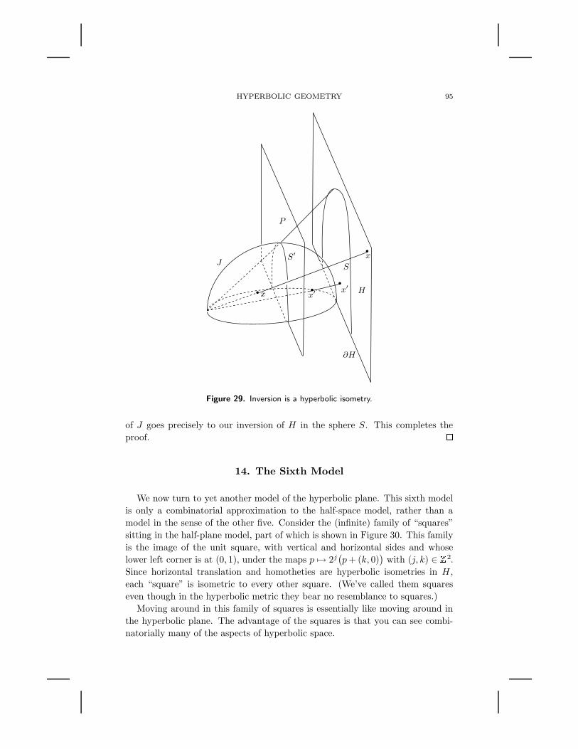
HYPERBOLIC GEOMETRY 95
••
•
•x
x
x′
x′
P
S
H
J
∂H
S′
Figure 29. Inversion is a hyperbolic isometry.
of J goes precisely to our inversion of H in the sphere S. This completes the
proof. �
14. The Sixth Model
We now turn to yet another model of the hyperbolic plane. This sixth model
is only a combinatorial approximation to the half-space model, rather than a
model in the sense of the other five. Consider the (infinite) family of “squares”
sitting in the half-plane model, part of which is shown in Figure 30. This family
is the image of the unit square, with vertical and horizontal sides and whose
lower left corner is at (0, 1), under the maps p 7→ 2j(
p+ (k, 0))
with (j, k) ∈ � 2.
Since horizontal translation and homotheties are hyperbolic isometries in H ,
each “square” is isometric to every other square. (We’ve called them squares
even though in the hyperbolic metric they bear no resemblance to squares.)
Moving around in this family of squares is essentially like moving around in
the hyperbolic plane. The advantage of the squares is that you can see combi-
natorially many of the aspects of hyperbolic space.
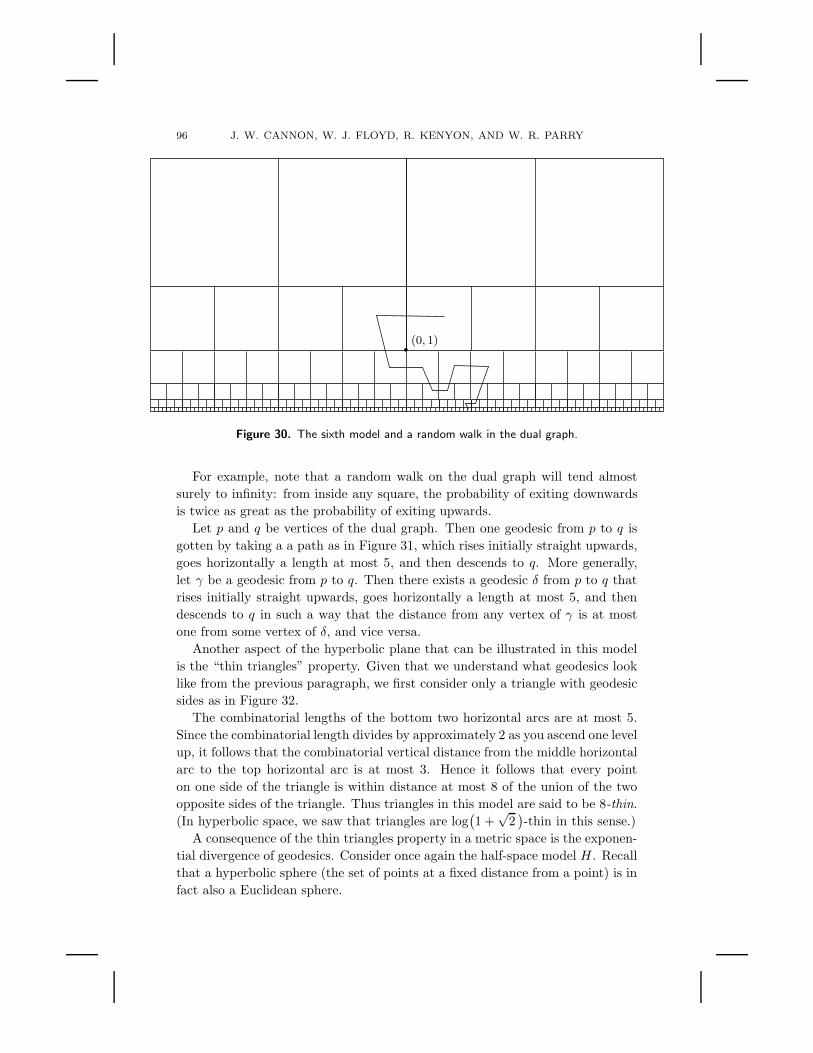
96 J. W. CANNON, W. J. FLOYD, R. KENYON, AND W. R. PARRY
•(0, 1)
Figure 30. The sixth model and a random walk in the dual graph.
For example, note that a random walk on the dual graph will tend almost
surely to infinity: from inside any square, the probability of exiting downwards
is twice as great as the probability of exiting upwards.
Let p and q be vertices of the dual graph. Then one geodesic from p to q is
gotten by taking a a path as in Figure 31, which rises initially straight upwards,
goes horizontally a length at most 5, and then descends to q. More generally,
let γ be a geodesic from p to q. Then there exists a geodesic δ from p to q that
rises initially straight upwards, goes horizontally a length at most 5, and then
descends to q in such a way that the distance from any vertex of γ is at most
one from some vertex of δ, and vice versa.
Another aspect of the hyperbolic plane that can be illustrated in this model
is the “thin triangles” property. Given that we understand what geodesics look
like from the previous paragraph, we first consider only a triangle with geodesic
sides as in Figure 32.
The combinatorial lengths of the bottom two horizontal arcs are at most 5.
Since the combinatorial length divides by approximately 2 as you ascend one level
up, it follows that the combinatorial vertical distance from the middle horizontal
arc to the top horizontal arc is at most 3. Hence it follows that every point
on one side of the triangle is within distance at most 8 of the union of the two
opposite sides of the triangle. Thus triangles in this model are said to be 8-thin.
(In hyperbolic space, we saw that triangles are log(
1 +√
2)
-thin in this sense.)
A consequence of the thin triangles property in a metric space is the exponen-
tial divergence of geodesics. Consider once again the half-space model H . Recall
that a hyperbolic sphere (the set of points at a fixed distance from a point) is in
fact also a Euclidean sphere.
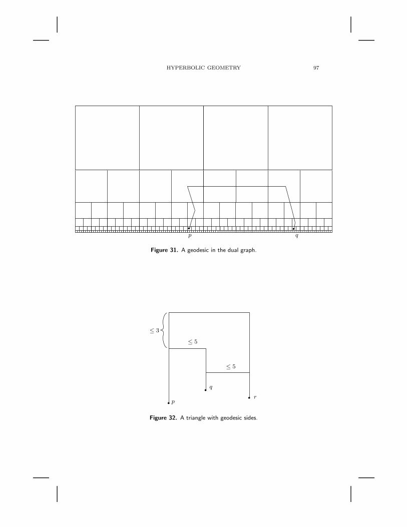
HYPERBOLIC GEOMETRY 97
••qp
Figure 31. A geodesic in the dual graph.
••
• p
q
r
≤ 3
≤ 5
≤ 5
Figure 32. A triangle with geodesic sides.

98 J. W. CANNON, W. J. FLOYD, R. KENYON, AND W. R. PARRY
H
∂H
Figure 33. A taxicab path. Integrate with respect to ds = � dx2 + dy2/y to
find the taxicab distance.
As in the proof of Fact 5 in Section 13, the area of a disk of radius rh is
Ah = 2π(cosh(rh) − 1),
whereas the length of the boundary of a disk of radius rh is 2πsinh(rh). For
large rh, these are both quite close to πerh , so in particular we see that the
circumference is exponential in the radius. This phenomenon will be known as
the exponential explosion, and is true in any metric space satisfying the thin
triangles condition.
Before we go on, we leave the reader with two exercises.
Exercise 1. Take a “taxicab” metric on H2 in which the allowed paths are
polygonal paths that have horizontal or vertical edges. See Figure 33. Analyze
the geodesics in this new metric, and prove the thin triangles property.
Exercise 2. Generalize the previous exercise to H3: let the allowed paths
be polygonal paths that are vertical (in the z-direction) or horizontal (lie par-
allel to the xy-plane). Define the length of a horizontal line segment to be
max{∆x,∆y}/z.
15. Why Study Hyperbolic Geometry?
Hyperbolic geometry and its geometric insights have application in diverse
areas of mathematics. The next three sections informally introduce some of
those applications. The material is intended to be skimmed, since the reader
may be unfamiliar with some of the prerequisite background material.
Hyperbolic geometry arises in three main areas:
(i) Complex variables and conformal mappings. In fact, work on automorphic
functions was Poincare’s original motivation for defining hyperbolic space; see
the quotation on page 63.
(ii) Topology (of three-manifolds in particular). More on this later regarding
Thurston’s surprising geometrization conjecture.
(iii) Group theory, in particular combinatorial group theory a la Gromov.

HYPERBOLIC GEOMETRY 99
Historically, hyperbolic geometry lies at the center of a triangle around which
revolve these three topics. See Figure 34. By using hard theorems in one domain
and hard connections between domains, one can prove surprising results.
One such example is the Mostow rigidity theorem [1973], which we quote here
in its simplest, lowest-dimensional form, for oriented, connected, compact three-
dimensional manifolds. To state the theorem we need a definition: a hyperbolic
structure on an n-dimensional manifold M is a Riemannian metric on M such
that the universal covering space of M is isometric to hyperbolic space Hn.
Theorem 15.1. Suppose the three-manifolds M1 and M2 having hyperbolic
structures are homotopy equivalent . Then M1 and M2 are in fact isometric.
Hyperbolicgeometry
Complex variablesConformal mapping
Topology
Group theory
Isometric linearfractional transformations
UniformizationAutomorphic forms
Thurston’sgeometrization
Mostowrigidity
Manifolds ofconstant curvature
Negativelycurved groups
Isometrygroups
Kleiniangroups
Fundamentalgroups
Riemann surfaces
Figure 34. Connections between hyperbolic geometry and the three areas.

100 J. W. CANNON, W. J. FLOYD, R. KENYON, AND W. R. PARRY
Here is a very abbreviated outline of the proof. There is an approximate metric
correspondence between the universal covering space of M1, as realized by hyper-
bolic space H3, and the fundamental group π1(M1), as realized geometrically by
its Cayley group graph. Likewise the universal cover of M2 and the Cayley graph
of π1(M2) are approximately isometric. The isomorphism between the funda-
mental groups π1(M1) and π1(M2) relates the two Cayley graphs metrically, and
consequently gives an approximate geometric mapping from H3, viewed as one
universal cover, back to H3 itself, viewed as the other universal cover. This map-
ping relates the actions of the two groups on their universal covers with enough
precision that it matches their actions on the two-sphere at infinity homeomor-
phically. It remains to prove that this correspondence at infinity is not only
homeomorphic but exactly conformal; the proof uses the theory of quasiconfor-
mal mappings and ergodicity of the group actions on the two-sphere at infinity.
When the most general theorem is proved, the details fill a book.
A corollary to this result is that the hyperbolic structure on a three-manifold
is a topological invariant. Consequently, so also are hyperbolic volume, lengths
of geodesics, etc.
The proof of Mostow Rigidity suggests that many important properties of
hyperbolic geometry are retained by spaces that only approximate hyperbolic
geometry. The case in point involves the Cayley graphs of the fundamental
groups, which are only one-dimensional and are not even manifolds, yet give a
good approximation to three-dimensional hyperbolic geometry in the large. We
shall return to this point when we describe Gromov’s word-hyperbolic groups.
But first we make precise the notion of spaces that are metrically comparable in
the large, or quasi-isometric. We start by recalling some definitions.
A group action of a group G on a space X is a map α : G×X → X , denoted
α(g, x) = g(x), such that 1(x) = x for all x ∈ X , and (g1g2)(x) = g1(g2(x)) for
all g1, g2 ∈ G and x ∈ X . In other words, α is a homomorphism from G into
Homeo(X).
A geometry is a path metric space in which metric balls are compact.
A geometric action of a group G on a geometry X is a group action that
satisfies the following conditions:
(i) G acts by isometries of X .
(ii) The action is properly discontinuous; that is, for every compact set Y ⊂ X ,
the set {g ∈ G : g(Y ) ∩ Y 6= � } has finite cardinality.
(iii) The quotient X/G = {xG : x ∈ X} is compact in the quotient topology.
Two geometries X1, X2 are quasi-isometric if there exist (not necessarily contin-
uous) functions R : X1 → X2, S : X2 → X1 and a positive real number M such
that
(i) S ◦R : X1 → X1 and R ◦ S : X2 → X2 are within M of the identities.
(ii) For all x1, y1 ∈ X1, d(R(x1), R(y1)) ≤Md(x1, y1) +M and likewise for X2.
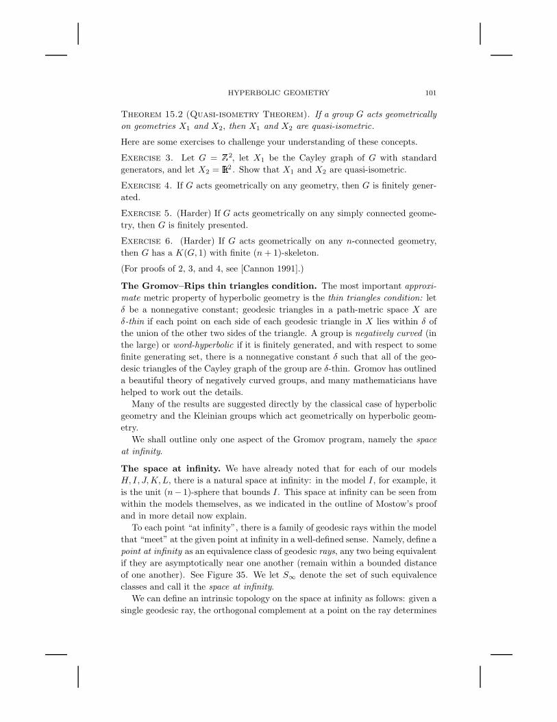
HYPERBOLIC GEOMETRY 101
Theorem 15.2 (Quasi-isometry Theorem). If a group G acts geometrically
on geometries X1 and X2, then X1 and X2 are quasi-isometric.
Here are some exercises to challenge your understanding of these concepts.
Exercise 3. Let G = � 2, let X1 be the Cayley graph of G with standard
generators, and let X2 =� 2 . Show that X1 and X2 are quasi-isometric.
Exercise 4. If G acts geometrically on any geometry, then G is finitely gener-
ated.
Exercise 5. (Harder) If G acts geometrically on any simply connected geome-
try, then G is finitely presented.
Exercise 6. (Harder) If G acts geometrically on any n-connected geometry,
then G has a K(G, 1) with finite (n+ 1)-skeleton.
(For proofs of 2, 3, and 4, see [Cannon 1991].)
The Gromov–Rips thin triangles condition. The most important approxi-
mate metric property of hyperbolic geometry is the thin triangles condition: let
δ be a nonnegative constant; geodesic triangles in a path-metric space X are
δ-thin if each point on each side of each geodesic triangle in X lies within δ of
the union of the other two sides of the triangle. A group is negatively curved (in
the large) or word-hyperbolic if it is finitely generated, and with respect to some
finite generating set, there is a nonnegative constant δ such that all of the geo-
desic triangles of the Cayley graph of the group are δ-thin. Gromov has outlined
a beautiful theory of negatively curved groups, and many mathematicians have
helped to work out the details.
Many of the results are suggested directly by the classical case of hyperbolic
geometry and the Kleinian groups which act geometrically on hyperbolic geom-
etry.
We shall outline only one aspect of the Gromov program, namely the space
at infinity.
The space at infinity. We have already noted that for each of our models
H, I, J,K,L, there is a natural space at infinity: in the model I , for example, it
is the unit (n− 1)-sphere that bounds I . This space at infinity can be seen from
within the models themselves, as we indicated in the outline of Mostow’s proof
and in more detail now explain.
To each point “at infinity”, there is a family of geodesic rays within the model
that “meet” at the given point at infinity in a well-defined sense. Namely, define a
point at infinity as an equivalence class of geodesic rays, any two being equivalent
if they are asymptotically near one another (remain within a bounded distance
of one another). See Figure 35. We let S∞ denote the set of such equivalence
classes and call it the space at infinity.
We can define an intrinsic topology on the space at infinity as follows: given a
single geodesic ray, the orthogonal complement at a point on the ray determines
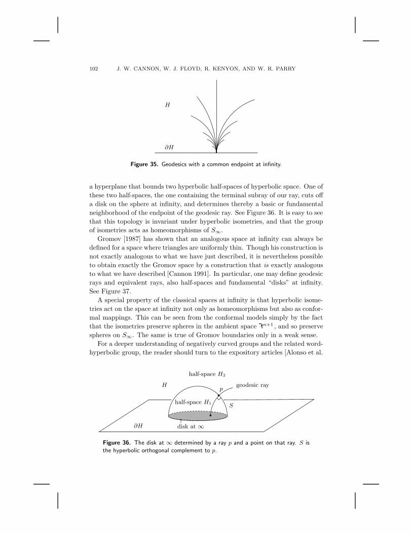
102 J. W. CANNON, W. J. FLOYD, R. KENYON, AND W. R. PARRY
H
∂H
Figure 35. Geodesics with a common endpoint at infinity.
a hyperplane that bounds two hyperbolic half-spaces of hyperbolic space. One of
these two half-spaces, the one containing the terminal subray of our ray, cuts off
a disk on the sphere at infinity, and determines thereby a basic or fundamental
neighborhood of the endpoint of the geodesic ray. See Figure 36. It is easy to see
that this topology is invariant under hyperbolic isometries, and that the group
of isometries acts as homeomorphisms of S∞.
Gromov [1987] has shown that an analogous space at infinity can always be
defined for a space where triangles are uniformly thin. Though his construction is
not exactly analogous to what we have just described, it is nevertheless possible
to obtain exactly the Gromov space by a construction that is exactly analogous
to what we have described [Cannon 1991]. In particular, one may define geodesic
rays and equivalent rays, also half-spaces and fundamental “disks” at infinity.
See Figure 37.
A special property of the classical spaces at infinity is that hyperbolic isome-
tries act on the space at infinity not only as homeomorphisms but also as confor-
mal mappings. This can be seen from the conformal models simply by the fact
that the isometries preserve spheres in the ambient space� n+1 , and so preserve
spheres on S∞. The same is true of Gromov boundaries only in a weak sense.
For a deeper understanding of negatively curved groups and the related word-
hyperbolic group, the reader should turn to the expository articles [Alonso et al.
•
↑•
H
S
p
∂H
geodesic ray
half-space H2
half-space H1
disk at ∞
Figure 36. The disk at ∞ determined by a ray p and a point on that ray. S is
the hyperbolic orthogonal complement to p.
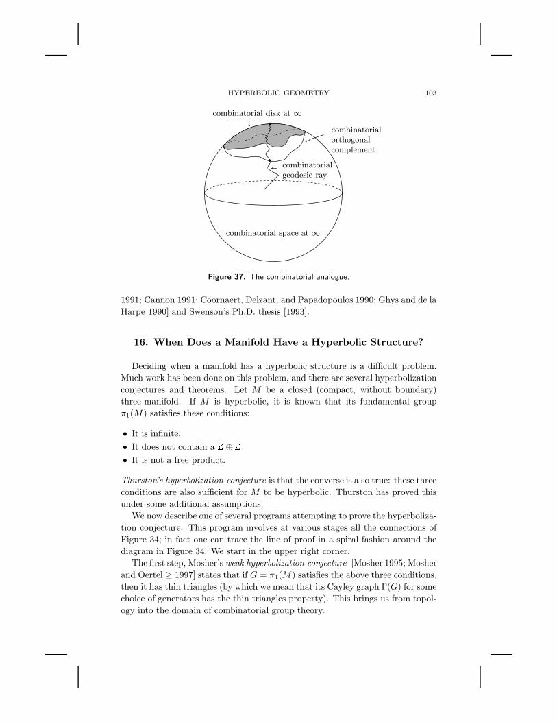
HYPERBOLIC GEOMETRY 103
•
•
←
←
↓combinatorial disk at ∞
combinatorialorthogonalcomplement
combinatorial space at ∞
combinatorialgeodesic ray
Figure 37. The combinatorial analogue.
1991; Cannon 1991; Coornaert, Delzant, and Papadopoulos 1990; Ghys and de la
Harpe 1990] and Swenson’s Ph.D. thesis [1993].
16. When Does a Manifold Have a Hyperbolic Structure?
Deciding when a manifold has a hyperbolic structure is a difficult problem.
Much work has been done on this problem, and there are several hyperbolization
conjectures and theorems. Let M be a closed (compact, without boundary)
three-manifold. If M is hyperbolic, it is known that its fundamental group
π1(M) satisfies these conditions:
• It is infinite.
• It does not contain a � ⊕ � .
• It is not a free product.
Thurston’s hyperbolization conjecture is that the converse is also true: these three
conditions are also sufficient for M to be hyperbolic. Thurston has proved this
under some additional assumptions.
We now describe one of several programs attempting to prove the hyperboliza-
tion conjecture. This program involves at various stages all the connections of
Figure 34; in fact one can trace the line of proof in a spiral fashion around the
diagram in Figure 34. We start in the upper right corner.
The first step, Mosher’s weak hyperbolization conjecture [Mosher 1995; Mosher
and Oertel ≥ 1997] states that if G = π1(M) satisfies the above three conditions,
then it has thin triangles (by which we mean that its Cayley graph Γ(G) for some
choice of generators has the thin triangles property). This brings us from topol-
ogy into the domain of combinatorial group theory.

104 J. W. CANNON, W. J. FLOYD, R. KENYON, AND W. R. PARRY
Note that in a group G with the thin triangles property you can define the
space at infinity ∂G, whose points are equivalence classes of geodesics (in Γ(G))
staying a bounded distance apart.
Assuming additionally that π1(M) has boundary homeomorphic to S2, we
attempt to equip this sphere with a conformal structure on which π1(M) acts
uniformly quasiconformally. This would bring the problem into the domain of
conformal mappings.
We would then apply a result of Sullivan and Tukia to conclude that the group
acts conformally for another conformal structure, quasiconformally equivalent to
this one.
Conformal self-maps of S2 extend to hyperbolic isometries of H3 (in the disk
model I). This would then give us, by taking the quotient, a hyperbolic manifold
(actually, an orbifold) M ′ homotopy equivalent to M .
Gabai and collaborators [Gabai 1994a; Gabai 1994b; Gabai, Meyerhoff, and
Thurston 1996] are extending Mostow rigidity to show that a three-manifold
homotopy equivalent to a hyperbolic three-manifold M ′ is in fact homeomorphic
to M ′.
So this would complete the program. Unfortunately many gaps remain to be
bridged.
Our current focus is on the construction of a conformal structure assuming
π1(M) has thin triangles and the space at infinity is homeomorphic to S2. We
have the following theorem (the converse of what we’d like to prove):
Theorem 16.1. Suppose a group G acts geometrically on H3. Then:
1. G is finitely generated .
2. Γ = Γ(G) (the Cayley graph for some choice of generators) has thin triangles .
3. ∂Γ ∼= S2.
Conjecture 16.2. The converse holds .
Here is the intuition behind parts 2 and 3 in Theorem 16.1. The group G acts
geometrically on Γ and on H3. By the quasi-isometry theorem, H3 and Γ are
quasi-isometric.
Consequently, the image in H3 of a geodesic in Γ looks “in the large” like a
geodesic with a linear factor of inefficiency. To avoid exponential inefficiency, it
must stay within a bounded distance of some genuine geodesic.
Any triangle in Γ will map to a thin triangle in H3, and hence is thin itself,
which proves condition 2. Condition 3 is established similarly.
To understand the difficulty in proving the conjecture, we have to appreciate
the difference between constant and variable negative sectional curvature.
Consider the following example, which illustrates a variable negative curvature
space. In the spaceK3 = {(x, y, z) : z > 0}, consider the paths that are piecewise
vertical (in the z-direction) or horizontal (parallel to the xy-plane). Use the met-
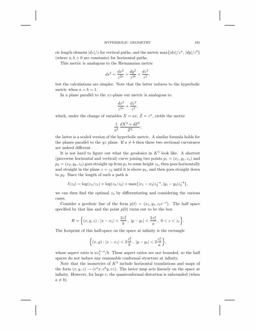
HYPERBOLIC GEOMETRY 105
ric length element |dz|/z for vertical paths, and the metric max{|dx|/za, |dy|/zb}(where a, b > 0 are constants) for horizontal paths.
This metric is analogous to the Riemannian metric
ds2 =dx2
z2a+dy2
z2b+dz2
z2,
but the calculations are simpler. Note that the latter reduces to the hyperbolic
metric when a = b = 1.
In a plane parallel to the xz-plane our metric is analogous to
dx2
z2a+dz2
z2,
which, under the change of variables X = ax, Z = za, yields the metric
1
a2
dX2 + dZ2
Z2;
the latter is a scaled version of the hyperbolic metric. A similar formula holds for
the planes parallel to the yz plane. If a 6= b then these two sectional curvatures
are indeed different.
It is not hard to figure out what the geodesics in K3 look like. A shortest
(piecewise horizontal and vertical) curve joining two points p1 = (x1, y1, z1) and
p2 = (x2, y2, z2) goes straight up from p1 to some height z3, then goes horizontally
and straight in the plane z = z3 until it is above p2, and then goes straight down
to p2. Since the length of such a path is
`(z3) = log(z3/z1) + log(z3/z2) + max{|x1 − x2|z−a3 , |y1 − y2|z−b
3 },
we can then find the optimal z3 by differentiating and considering the various
cases.
Consider a geodesic line of the form p(t) = (x1, y1, z1e−t). The half space
specified by that line and the point p(0) turns out to be the box
B ={
(x, y, z) : |x− x1| <2zb
1
b, |y − y1| <
2za1
a, 0 < z < z1
}
.
The footprint of this half-space on the space at infinity is the rectangle
{
(x, y) : |x− x1| < 2zb1
b, |y − y1| < 2
za1
a
}
,
whose aspect ratio is azb−a1 /b. These aspect ratios are not bounded, so the half
spaces do not induce any reasonable conformal structure at infinity.
Note that the isometries of K3 include horizontal translations and maps of
the form (x, y, z) → (vax, vby, vz). The latter map acts linearly on the space at
infinity. However, for large v, the quasiconformal distortion is unbounded (when
a 6= b).
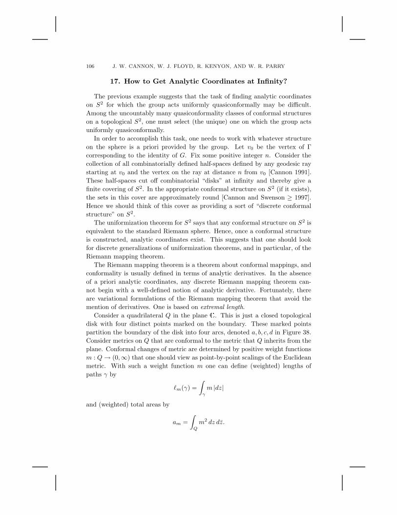
106 J. W. CANNON, W. J. FLOYD, R. KENYON, AND W. R. PARRY
17. How to Get Analytic Coordinates at Infinity?
The previous example suggests that the task of finding analytic coordinates
on S2 for which the group acts uniformly quasiconformally may be difficult.
Among the uncountably many quasiconformality classes of conformal structures
on a topological S2, one must select (the unique) one on which the group acts
uniformly quasiconformally.
In order to accomplish this task, one needs to work with whatever structure
on the sphere is a priori provided by the group. Let v0 be the vertex of Γ
corresponding to the identity of G. Fix some positive integer n. Consider the
collection of all combinatorially defined half-spaces defined by any geodesic ray
starting at v0 and the vertex on the ray at distance n from v0 [Cannon 1991].
These half-spaces cut off combinatorial “disks” at infinity and thereby give a
finite covering of S2. In the appropriate conformal structure on S2 (if it exists),
the sets in this cover are approximately round [Cannon and Swenson ≥ 1997].
Hence we should think of this cover as providing a sort of “discrete conformal
structure” on S2.
The uniformization theorem for S2 says that any conformal structure on S2 is
equivalent to the standard Riemann sphere. Hence, once a conformal structure
is constructed, analytic coordinates exist. This suggests that one should look
for discrete generalizations of uniformization theorems, and in particular, of the
Riemann mapping theorem.
The Riemann mapping theorem is a theorem about conformal mappings, and
conformality is usually defined in terms of analytic derivatives. In the absence
of a priori analytic coordinates, any discrete Riemann mapping theorem can-
not begin with a well-defined notion of analytic derivative. Fortunately, there
are variational formulations of the Riemann mapping theorem that avoid the
mention of derivatives. One is based on extremal length.
Consider a quadrilateral Q in the plane � . This is just a closed topological
disk with four distinct points marked on the boundary. These marked points
partition the boundary of the disk into four arcs, denoted a, b, c, d in Figure 38.
Consider metrics on Q that are conformal to the metric that Q inherits from the
plane. Conformal changes of metric are determined by positive weight functions
m : Q→ (0,∞) that one should view as point-by-point scalings of the Euclidean
metric. With such a weight function m one can define (weighted) lengths of
paths γ by
`m(γ) =
∫
γ
m |dz|
and (weighted) total areas by
am =
∫
Q
m2 dz dz.
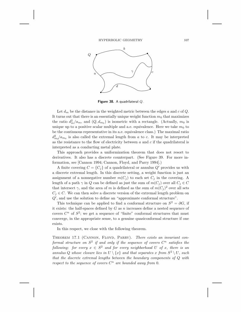
HYPERBOLIC GEOMETRY 107
•
••
•
γ
Q
a
b
c
d
Figure 38. A quadrilateral Q.
Let dm be the distance in the weighted metric between the edges a and c of Q.
It turns out that there is an essentially unique weight functionm0 that maximizes
the ratio d2m/am, and (Q, dm0
) is isometric with a rectangle. (Actually, m0 is
unique up to a positive scalar multiple and a.e. equivalence. Here we take m0 to
be the continuous representative in its a.e. equivalence class.) The maximal ratio
d2m0/am0
is also called the extremal length from a to c. It may be interpreted
as the resistance to the flow of electricity between a and c if the quadrilateral is
interpreted as a conducting metal plate.
This approach provides a uniformization theorem that does not resort to
derivatives. It also has a discrete counterpart. (See Figure 39. For more in-
formation, see [Cannon 1994; Cannon, Floyd, and Parry 1994].)
A finite covering C = {Cj} of a quadrilateral or annulus Q′ provides us with
a discrete extremal length. In this discrete setting, a weight function is just an
assignment of a nonnegative number m(Cj) to each set Cj in the covering. A
length of a path γ in Q can be defined as just the sum of m(Cj) over all Cj ∈ C
that intersect γ, and the area of m is defined as the sum of m(Cj)2 over all sets
Cj ∈ C. We can then solve a discrete version of the extremal length problem on
Q′, and use the solution to define an “approximate conformal structure”.
This technique can be applied to find a conformal structure on S2 = ∂G, if
it exists: the half-spaces defined by G as n increases define a nested sequence of
covers Cn of S2; we get a sequence of “finite” conformal structures that must
converge, in the appropriate sense, to a genuine quasiconformal structure if one
exists.
In this respect, we close with the following theorem.
Theorem 17.1 (Cannon, Floyd, Parry). There exists an invariant con-
formal structure on S2 if and only if the sequence of covers Cn satisfies the
following : for every x ∈ S2 and for every neighborhood U of x, there is an
annulus Q whose closure lies in U \ {x} and that separates x from S2 \ U , such
that the discrete extremal lengths between the boundary components of Q with
respect to the sequence of covers Cn are bounded away from 0.
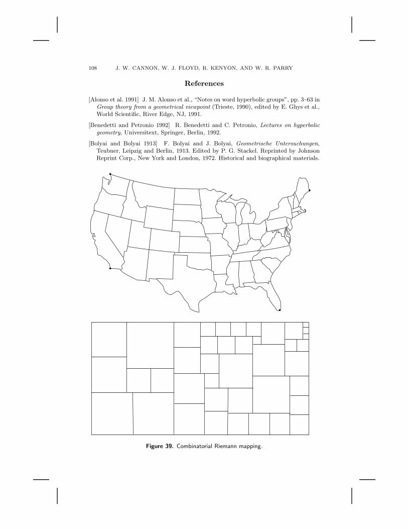
108 J. W. CANNON, W. J. FLOYD, R. KENYON, AND W. R. PARRY
References
[Alonso et al. 1991] J. M. Alonso et al., “Notes on word hyperbolic groups”, pp. 3–63 inGroup theory from a geometrical viewpoint (Trieste, 1990), edited by E. Ghys et al.,World Scientific, River Edge, NJ, 1991.
[Benedetti and Petronio 1992] R. Benedetti and C. Petronio, Lectures on hyperbolicgeometry, Universitext, Springer, Berlin, 1992.
[Bolyai and Bolyai 1913] F. Bolyai and J. Bolyai, Geometrische Untersuchungen,Teubner, Leipzig and Berlin, 1913. Edited by P. G. Stackel. Reprinted by JohnsonReprint Corp., New York and London, 1972. Historical and biographical materials.
•
•
•
•
Figure 39. Combinatorial Riemann mapping.
HYPERBOLIC GEOMETRY 109
[Cannon 1991] J. W. Cannon, “The theory of negatively curved spaces and groups”,pp. 315–369 in Ergodic theory, symbolic dynamics and hyperbolic spaces, edited byT. Bedford et al., Oxford U. Press, Oxford, 1991.
[Cannon 1994] J. W. Cannon, “The combinatorial Riemann mapping theorem”, ActaMath. 173 (1994), 155–234.
[Cannon et al. 1994] J. W. Cannon, W. J. Floyd, and W. R. Parry, “Squaring rectangles:the finite Riemann mapping theorem”, pp. 133–212 in The mathematical legacy ofWilhelm Magnus: groups, geometry and special functions (Brooklyn, NY, 1992),edited by W. Abikoff et al., Contemporary Mathematics 169, Amer. Math. Soc.,Providence, 1994.
[Cannon and Swenson ≥ 1998] J. W. Cannon and E. L. Swenson, “Recognizing constantcurvature groups in dimension 3”. Preprint.
[Coornaert et al. 1990] M. Coornaert, T. Delzant, and A. Papadopoulos, Geometrie ettheorie des groupes: les groupes hyperboliques de Gromov, Lecture Notes in Math.1441, Springer, Berlin, 1990.
[Euclid 1926] Euclid, The Thirteen Books of Euclid’s Elements, second ed., CambridgeU. Press, Cambridge, 1926. Edited by T. L. Heath. Reprinted by Dover, New York,1956.
[Gabai 1994a] D. Gabai, “Homotopy hyperbolic 3-manifolds are virtually hyperbolic”,J. Amer. Math. Soc. 7 (1994), 193–198.
[Gabai 1994b] D. Gabai, “On the geometric and topological rigidity of hyperbolic3-manifolds”, Bull. Amer. Math. Soc. (N.S.) 31 (1994), 228–232.
[Gabai et al. 1996] D. Gabai, R. Meyerhoff, and N. Thurston, “Homotopy hyperbolic 3-manifolds are hyperbolic”, 1996. Available at http://www.msri.org/MSRI-preprints/online/1996-058.
[Ghys and de la Harpe 1990] E. Ghys and P. de la Harpe, Sur les groupes hyperboliquesd’apres Mikhael Gromov, Birkhauser, boston, 1990.
[Gromov 1987] M. L. Gromov, “Hyperbolic groups”, pp. 75–263 in Essays in grouptheory, edited by S. Gersten, MSRI Publications 8, Springer, New York, 1987.Perhaps the most influential recent paper in geometric group theory.
[Hilbert and Cohn-Vossen 1932] D. Hilbert and S. Cohn-Vossen, AnschaulicheGeometrie, Grundlehren der math. Wissenschaften 37, Springer, Berlin, 1932.Reprinted by Dover, New York, 1944. Translated by Paul Nemenyi as Geometryand the Imagination, Chelsea, New York, 1952. College-level exposition of rich ideasfrom low-dimensional geometry, with many figures.
[Iversen 1993] B. Iversen, Hyperbolic geometry, London Math. Soc. Student Texts 25,Cambridge U. Press, Cambridge, 1993. Very clean algebraic approach to hyperbolicgeometry.
[Klein 1928] F. Klein, Vorlesungen uber nicht-Euklidische Geometrie, Grundlehrender math. Wissenschaften 26, Springer, Berlin, 1928. Edited by W. Rosemann.Reprinted by Chelsea, New York, 1960. Mostly algebraic development of non-Euclidean geometry with respect to Klein and projective models. Beautiful figures.Elegant exposition.
110 J. W. CANNON, W. J. FLOYD, R. KENYON, AND W. R. PARRY
[Kline 1972] M. Kline, Mathematical thought from ancient to modern times, OxfordU. Press, New York, 1972. A well-written and fairly concise history of mathematics(1200 pages in one or three volumes). Full of interesting material.
[Lobachevskiı 1898] N. I. Lobachevskiı, Zwei geometrische Abhandlungen, Bibliothecamath. Teubneriana 70, Teubner, Leipzig, 1898. Reprinted by Johnson Reprint Corp.,New York and London, 1972. Original papers.
[Mosher 1995] L. Mosher, “Geometry of cubulated 3-manifolds”, Topology 34 (1995),789–814.
[Mosher and Oertel ≥ 1998] L. Mosher and U. Oertel, “Spaces which are not negativelycurved”. Preprint.
[Poincare 1908] H. Poincare, Science et methode, E. Flammarion, Paris, 1908.Translated by F. Maitland as Science and method, T. Nelson and Sons, London,1914. Reprinted by Dover, New York, 1952, and by Thoemmes Press, Bristol, 1996.One of Poincare’s several popular expositions of science. Still worth reading afteralmost 100 years.
[Ratcliffe 1994] J. G. Ratcliffe, Foundations of hyperbolic manifolds, Graduate Textsin Math. 149, Springer, New York, 1994. Fantastic bibliography, careful and unifiedexposition.
[Riemann 1854] G. F. B. Riemann, “Uber die Hypothesen, welche der Geometrie zuGrunde liegen”, Konigliche Gesellschaft der Wissenschaften zu Gottingen 13 (1854),1–20. Also pp. 272–287 in Gesammelte Mathematische Werke, edited by R. Dedekindand H. Weber, 2nd ed., Teubner, Leipzig, 1902 (reprint: Dover, New York, 1953).
[Swenson 1993] E. L. Swenson, Negatively curved groups and related topics, Ph.D.thesis, Brigham Young University, 1993.
[Thurston 1997] W. P. Thurston, Three-dimensional geometry and Topology, PrincetonU. Press, Princeton, 1997. Thurston reintroduced hyperbolic geometry to thetopologist in the 1970s. This richly illustrated book has an accessible beginningand progresses to great and exciting heights.
[Weyl 1919] H. Weyl, Raum, Zeit, Materie: Vorlesungen uber allgemeine Rela-tivitatstheorie, Springer, Berlin, 1919. Translated by H. L. Brose as Space–Time–Matter, Dover, New York, 1922; reprinted 1950. Weyl’s exposition and developmentof relativity and gauge theory; begins at the beginning with motivation, philosophy,and elementary developments as well as advanced theory.
Index
action, 100Alonso, Juan M., 103analytic model, see modelangle
–s of a triangle, 61, 88–s, preservation of, see conformalin Riemannian manifold, 68interior, 60
applications of hyperbolic geometry, 59, 98approximate
conformal structure, see quasiconformalhyperbolic geometry, 100
approximationcombinatorial, 95Euclidean, 93
arclength, see also length element, 65area
element, 68, 89, 92
of circle, 92, 98of triangle, 88

HYPERBOLIC GEOMETRY 111
astral geometry, 61automorphic function, 63, 98axiomatic geometry, 59, 62
Beltrami Eugenio, 62Benedetti, Riccardo, 60Bolyai, Farkas (or Wolfgang), 62Bolyai, Janos (or Johann), 62
Caen, 63calculus, 65, 67Cannon, James W., 101–103, 106, 107Cauchy–Schwarz inequality, 67Cayley graph, 100, 101center
of circle, 60of sphere, 87
centralprojection, 71
circle, see also sphere, 60, 65hyperbolic, 92
circumference, 92, 98classification of isometries, 84Cohn-Vossen, Stephan, 74combinatorial
group theory, 60, 98, 103model, 95Riemann mapping, 107
compactification, 84complex
analysis, 60, 98conformal
map, 72, 98, 100, 102, 104, 106model, 63, 86structure, 104, 106, 107
discrete, 106congruence
of right angles, 60of triangles, 61
consistency of non-Euclidean geometry, 62constant
curvature, 62, 104speed, 65, 66
Coornaert, Michel, 103cosine, 65
hyperbolic, 66, 67, 83, 84, 98Coutances, 63curious facts, 86curvature, 60, 62, 104
Delzant, Thomas, 103
differential equation, 65disk model, 69, 71, 84, 89, 92, 101, 104
geodesics, 80distance, 69
element, see lengthin the half-space model, 90
Einstein, Albert, 59electricity, 107element
of area, 89, 92of length, 92
ellipticfunctions, 63isometry, 85
equidistant locus, 61, 88ergodic theory, 100Euclid, 59
–’s postulates, 60Euclidean
approximation, 93distance, 64geometry, 60, 62hyperbolic, 96inner product, 64–66, 85isometry, 79, 85, 86, 94line, 79, 88, 93, 94metric, 63, 73, 74, 106similarity, 94, 106sphere, 64, 86, 87, 93, 96
Euler, Leonhard, 62exponential explosion, 98extremal length, 106, 107
fifth postulate, see parallel postulatefixed point, 84, 85Floyd, William J., 107Fuchsian functions, 63fundamental group, 100
Gabai, David, 104Gauss, Carl Friedrich, 62Gauss–Bonnet theorem, 88–90geodesic, 77
existence of, 77in disk model, 80in half-space model, 77in hemisphere model, 80in hyperboloid model, 80in Klein model, 80

112 J. W. CANNON, W. J. FLOYD, R. KENYON, AND W. R. PARRY
length of, 100triangle, 101vertical, 78, 84, 88, 91
geometricaction, 100
geometry(type of metric space), 100
Ghys, Etienne, 103Gram–Schmidt orthogonalization, 68Gromov, Mikhael L., 98, 101, 102group
action, 100theory, see combinatorial group theory
H, 69Hn, 65half-space model, 69, 71, 86, 88, 90, 93, 94
geodesics, 77, 78Harpe, Pierre de la, 103hemisphere model, 69, 71, 72, 84, 86, 94
geodesics, 80Hilbert, David, 74history of non-Euclidean geometry, 60–62homotopy equivalence, 99hyperbolic, see also non-Euclidean
arclength, 66cosine, 66, 67, 83, 84, 98distance, 90Euclidean, 96geometry
applications of, 59, 98models, 60reason for name, 63
inner product, see Minkowski innerproduct
isometry, 86isometry (restricted sense), see loxo-
dromicline, 66model, 69orthogonality, 67sine, 66, 67, 98sphere, 86square, 95structure, 99, 103volume, 100
hyperbolization conjecture, 103hyperboloid, 64
model, 71, 84in projective space, 84
hyperboloid model, 69geodesics, 80
hypergeometric series, 63
I, 69ideal triangle, 89, 91identification of two sheets, 64indefinite
inner product, see Minkowski innerproduct
infinityfixed point at, 85space at, 84, 85, 87, 91, 93, 101, 104
analytic coordinates for, 106intrinsic definition, 101topology of, 101
vertex at, 89inner product
and Riemannian metric, 68Euclidean, 64–66, 85hyperbolic, see Minkowski inner prod-
uctindefinite, see Minkowski inner productMinkowski, 64–68, 82, 85positive definite, 67
interior angle, 60interior of the disk model, see disk modelinversion, 93–95isometric manifolds, 99isometry
between models, 71classification of –ies, 84equivalence between concepts, 82Euclidean, 86fixed points, 84hyperbolic, 86in hyperboloid model, 80linear, 80Riemannian, 82topological, 82
Iversen, Birger, 60
J , 69Jemisphere model, see hemisphere model
K, 69Kastner, Abraham Gotthelf, 61Klugel, Georg Simon, 61Klein model, 69, 71, 72, 84
geodesics, 80Klein, Felix, 60

HYPERBOLIC GEOMETRY 113
Kleinian functions, 63Kline, Morris, 60
L, 69Lambert, Johann Heinrich, 61length
element, 68, 92of geodesics, 100of path, 69of vector, 68
light cone, 64line, see also geodesic
is infinite, 60through two points, 60
linearisometry, 80, 82–84
conditions for, 82Lobachevskiı, Nikolaı Ivanovich, 62’loid model, see hyperboloid modelloxodromic
isometry, 85
manifold, 60, 68, 69, 98, 104Riemannian, 69
matrix of linear isometry, 82, 83, 85Meyerhoff, Robert, 104Minding, Ferdinand, 62Minkowski
inner product, 64–68, 82, 85model, 64
Minkowski, Hermann, 59mnemonic names for models, 69model, see also disk, half-space, hemi-
sphere, hyperboloid, Klein, 61–63, 69–s, isometries between, 71conformal, 63, 86domain of, 70Riemannian metric of, 71
Monge, Gaspard, 62Mosher, Lee, 103Mostow rigidity theorem, 99, 101
extensions of, 104Mostow, George D., 99
negative curvature, see also constant cur-vature, 60, 62
negatively curved group, 101non-Euclidean geometry, see also hyper-
bolicconsistency of, 62
history of, 60–62norm, see inner productnorth pole, 73
one-dimensional case, 65orbifold, 104orthogonal
complement, 67, 68, 78, 85, 101, 102transformation, 85, 86
orthogonalization, 68
Papadopoulos, Athanase, 103parabolic isometry, 85parallel postulate, 60–62
denial of, 61Parry, Walter R., 107path, see also shortest path, 65Petronio, Carlo, 60physics, 60Poincare, Henri, 63, 98pole, 73positive definite
inner product, 67, 68postulate
–s of Euclidean geometry, 60fifth, see parallel postulate
preservationof angles, see conformalof spheres, 75, 76
Proclus, 61projection
central, 71stereographic, 72, 74, 76, 86vertical, 71
projectiveidentification, 64space, 84
properly discontinuous, 100pullback, 68, 71, 72, 77
under stereographic projection, 73
quadrilateral, 61, 106quasi-isometry, 100
theorem, 101, 104quasiconformal, 100, 104, 106, 107
radius, 60, 88, 90, 94and circumference, 98imaginary, 64large, 92

114 J. W. CANNON, W. J. FLOYD, R. KENYON, AND W. R. PARRY
relation between hyperbolic and Eu-clidean, 92
randomwalk, 96
Ratcliffe, John G., 60ray, 101reflection, 94relativity, 64resistance, 107retraction, 78
principle, 77Riemann mapping theorem, 106Riemann, Georg Friedrich Bernhard, 62Riemannian
distance, 82, 83isometry, 82, 83manifold, 62, 69metric, 68, 82, 83
of models, 71right angle, 60Rips, Eliyahu, 101rudiments, 68
S∞, 101Saccheri, Girolamo, 61Schweikart, 61segment, see lineshortest path, see also geodesic, 77–79similarity of triangles, 61sine, 65
hyperbolic, 66, 67, 98south pole, 73space at infinity, see infinityspace-time, 60, 63, 64sphere
–s, preservation under stereographicprojection, 76
–s, preserved under stereographic pro-jection, 75
center of, 87Euclidean, 64, 86, 87, 93, 96hyperbolic, 86of radius i, 64
stereographicprojection, 72, 74, 76, 86, 94
straight line, see lineSullivan, Dennis, 104surfaces of constant negative curvature, 62Swenson, Eric L., 103, 106
Sylvester’s theorem, 68synthetic development, 62
tangent vector, 65–67Taurinus, 61taxicab geometry, 98teaching of calculus, 65, 67theta-Fuchsian functions, 63thin triangles condition, 90, 98, 101–103Thurston, Nathaniel J., 104Thurston, William P., 60, 77, 98, 103time
and space, see space-timetopological
invariant, 100isometry, 82, 83
topology, 60, 98triangle
area of, 88geodesic, 101ideal, 89, 91similar, 61sum of angles, 61, 88thinness, see thin triangles conditionwith specified angles, 90
trigonometry, 62Tukia, Pekka, 104
uniformization theorem, 106, 107unit
circle, 65hyperbola, 66sphere, 64
universal cover, 100upper half-space, see half-space
variable curvature, 104velocity, 65, 66vertical
geodesic, 78, 84, 88, 91projection, 71
volume, 100
Wallis, John, 61weak
hyperbolization conjecture, 103weight function, 106Weyl, Hermann, 67word-hyperbolic group, 101, 102
HYPERBOLIC GEOMETRY 115
James W. CannonDepartment of MathematicsBrigham Young UniversityProvo, UT 84602-1001
William J. FloydDepartment of MathematicsVirginia Polytechnical Institute and State UniversityBlacksburg, VA 24061-0123
Richard KenyonDepartement de MathematiquesEcole Normale Superieure de Lyon46, allee d’Italie, 69364 LyonFrance
Walter R. ParryDepartment of MathematicsEastern Michigan UniversityYpsilanti, MI 48197