hydrogeology and analysis of the ground-water-flow … · hydrogeology and analysis of the...

Hydrogeology and Analysis of the Ground-Water-Flow System of the Eastern Shore, Virginia

United States Geological SurveyWater-Supply Paper 2401

Prepared in cooperation witl Accomack County, Northampton County, and the Virginia Water Control Board


By DONNA L. RICHARDSON

Prepared in cooperation with Accomack County, Northampton County, and the Virginia Water Control Board

U.S. GEOLOGICAL SURVEY WATER-SUPPLY PAPER 2401

U.S. DEPARTMENT OF THE INTERIOR

BRUCE BABBITT, Secretary

U.S. GEOLOGICAL SURVEY

GORDON P. EATON, Director

Any use of trade, product, or firm names in this publication is for descriptive purposes only and does not imply endorsement by the U.S. Government.

Printed in the Eastern Region, Reston, Va.

UNITED STATES GOVERNMENT PRINTING OFFICE: 1994

For sale byU.S. Geological Survey, Map Distribution Box 25286, MS 306, Federal Center Denver, CO 80225

Library of Congress Cataloging in Publication Data

Richardson, Donna L.Hydrogeology and analysis of the ground-water-flow system of the Eastern

Shore, Virginia / by Donna L. Richardson.p. cm. (U.S. Geological Survey water-supply paper; 2401)

Includes bibliographical references. Supt. of Docs, no.: I 19.13: 1. Water, Underground Eastern Shore (Md. and Va.) 2. Groundwater

flow Eastern Shore (Md. and Va.) I. Title. II. Series. GB1025.V8R53 1994551.49'09755'1 -dc20 92-33725

CIP

CONTENTS

Abstract ..................................................................................................................................... 1Introduction................................................................................................................................. 2

Purpose and Scope................................................................................................................. 2Location of Study and Model Area............................................................................................. 3Previous Studies.................................................................................................................... 3Methods of Investigation ........................................................................................................ 4Acknowledgments ................................................................................................................. 4

Hydrogeology.............................................................................................................................. 4General Geology................................................................................................................... 4

Cretaceous Sediments...................................................................................................... 5Tertiary Sediments ......................................................................................................... 5Quaternary Sediments ..................................................................................................... 5

Aquifers and Confining Units ................................................................................................... 7Columbia Aquifer .......................................................................................................... 7Pleistocene Paleochannel Aquifers ...................................................................................... 18Yorktown-Eastover Aquifer System..................................................................................... 18

Upper Yorktown-Eastover Aquifer and Confining Unit...................................................... 20Middle Yorktown-Eastover Aquifer and Confining Unit .................................................... 20Lower Yorktown-Eastover Aquifer and Confining Unit..................................................... 20

St. Marys Confining Unit................................................................................................. 22Ground-Water Hydrology ........................................................................................................ 22

Local Ground-Water-Flow System ...................................................................................... 22Regional Ground-Water-Flow System .................................................................................. 23

Ground-Water Use................................................................................................................. 26Chloride Distribution.............................................................................................................. 33

Analysis of the Ground-Water-Flow System ......................................................................................... 33Development of the Flow Model................................................................................................ 33Model Grid and Boundaries...................................................................................................... 46Model Calibration.................................................................................................................. 48

Transmissivity............................................................................................................... 50Storage Coefficient......................................................................................................... 50Vertical Leakance .......................................................................................................... 50

Steady-State-Model Simulation of Prepumping Conditions ................................................................ 50Transient-Model Simulation of Pumping Conditions ........................................................................ 61

Time Discretization and Ground-Water Withdrawals ................................................................ 61Results of Simulation...................................................................................................... 61

Application of Ground-Water-Flow Model.................................................................................... 71Southern Northampton County Scenario ............................................................................... 71

Simulation 1 ......................................................................................................... 71Simulation 2 ......................................................................................................... 81

Northeastern Accomack County Scenario.............................................................................. 85Simulation 1: No-Flow Boundary................................................................................ 85Simulation 2: Constant-Head Boundary......................................................................... 87

Permitted-Withdrawal Scenario .......................................................................................... 94Discussion of Model Results..................................................................................................... 95Sensitivity Analysis................................................................................................................ 100

Contents III

Model Limitations ................................................................................................................. 100Summary.................................................................................................................................... 106References Cited........................................................................................................................... 107

PLATE[In pocket]

I. Hydrogeologic sections for the Eastern Shore, Virginia

FIGURES

1. Map showing location of study and model area.......................................................................... 32. Map showing location of control wells used in hydrogeologic framework analysis ............................... 6

3-9. Hydrogeologic maps showing altitude of top of:3. Upper Yorktown-Eastover confining unit............................................................................ 104. Upper Yorktown-Eastover aquifer .................................................................................... 115. Middle Yorktown-Eastover confining unit........................................................................... 126. Middle Yorktown-Eastover aquifer ................................................................................... 137. Lower Yorktown-Eastover confining unit ........................................................................... 148. Lower Yorktown-Eastover aquifer .................................................................................... 159. St. Marys confining unit................................................................................................ 16

10. Schematic diagram of aquifers and confining units and generalized flow lines..................................... 17II,12. Maps showing:

11. Bathymetry in the vicinity of the Eastern Shore.................................................................... 2112. Locations of wells along transect A-A' in the Columbia aquifer................................................ 24

13,14. Graphs showing:13. Water levels in selected wells along a transect A-A' in the Columbia aquifer ............................... 2514. Water levels in an irrigation pond and in a nearby well completed in the Columbia aquifer .............. 26

15. Map showing location of selected Virginia Water Control Board research-station well clusters ................ 2716. Graphs of water levels in research-station well clusters (A) in a recharge area and (B) in a discharge area .. 3017. Map showing location of observation wells and chloride concentrations in the upper Potomac aquifer for

the Coastal Plain of Virginia................................................................................................. 3118. Graph showing annual ground-water withdrawal from model area ................................................... 32

19-22. Maps showing chloride concentrations in:19. Columbia aquifer......................................................................................................... 3420. Upper Yorktown-Eastover aquifer .................................................................................... 3521. Middle Yorktown-Eastover aquifer ................................................................................... 3622. Lower Yorktown-Eastover aquifer.................................................................................... 37

23. Schematic diagram of model representation of the saltwater-freshwater interface tip and toe ................... 4624. Map showing finite-difference grid and boundaries used in model analysis......................................... 4725. Schematic diagram showing physical and model conceptualizations of ground-water-flow system............. 4826. Map showing average water levels for the Columbia aquifer.......................................................... 49

27-29. Maps showing hydraulic conductivity based on model calibration:27. Upper Yorktown-Eastover aquifer .................................................................................... 5128. Middle Yorktown-Eastover aquifer ................................................................................... 5229. Lower Yorktown-Eastover aquifer .................................................................................... 53

30-32. Maps showing simulated prepumping water levels in:30. Upper Yorktown-Eastover aquifer .................................................................................... 5531. Middle Yorktown-Eastover aquifer ................................................................................... 5632. Lower Yorktown-Eastover aquifer.................................................................................... 57

33-35. Maps showing simulated prepumping position of the saltwater-freshwater interface for:33. Upper Yorktown-Eastover aquifer .................................................................................... 5834. Middle Yorktown-Eastover aquifer ................................................................................... 5935. Lower Yorktown-Eastover aquifer.................................................................................... 60

36. Graph showing estimated annual withdrawal and average withdrawal for simulated pumping periods......... 62

IV Contents

37-39. Graphs showing simulated and measured water levels at selected observation wells in:37. Upper Yorktown-Eastover aquifer .................................................................................... 6438. Middle Yorktown-Eastover aquifer ................................................................................... 6539. Lower Yorktown-Eastover aquifer.................................................................................... 66

40-42. Maps showing simulated and measured water levels for 1988 in:40. Upper Yorktown-Eastover aquifer .................................................................................... 6741. Middle Yorktown-Eastover aquifer ................................................................................... 6842. Lower Yorktown-Eastover aquifer.................................................................................... 69

43-45. Maps showing simulated position of the saltwater-freshwater interface toe for a 1,000-year transient run using 1988 withdrawals in:43. Upper Yorktown-Eastover aquifer .................................................................................... 7244. Middle Yorktown-Eastover aquifer ................................................................................... 7345. Lower Yorktown-Eastover aquifer.................................................................................... 74

46. Map showing location of hypothetical withdrawals for the southern Northampton County scenario,simulation 1..................................................................................................................... 75

47. Map showing water-level decline from simulated 1988 water levels, simulated position of thesaltwater-freshwater interface toe, and area of reversed saltwater flow in the upper Yorktown-Eastover aquifer, southern Northampton County scenario, simulation 1 ........................................................ 78

48,49. Maps showing water-level decline from simulated 1988 water levels and simulated position of the saltwater-freshwater interface toe for the southern Northampton County scenario, simulation 1, in:48. Middle Yorktown-Eastover aquifer ................................................................................... 7949. Lower Yorktown-Eastover aquifer.................................................................................... 80

50-52. Maps showing water-level decline from simulated 1988 water levels and simulated position of the saltwater-freshwater interface toe for the southern Northampton County scenario, simulation 2, in:50. Upper Yorktown-Eastover aquifer .................................................................................... 8251. Middle Yorktown-Eastover aquifer ................................................................................... 8352. Lower Yorktown-Eastover aquifer .................................................................................... 84

53. Map showing location of hypothetical withdrawals in the northeastern Accomack County scenarios .......... 8654. Map showing water-level decline from simulated 1988 water levels, simulated position of the

saltwater-freshwater interface toe, and area of reversed saltwater flow in the upper Yorktown-Eastover aquifer, northeastern Accomack County scenario, simulation 1....................................................... 88

55,56. Maps showing water-level decline from simulated 1988 water levels and simulated position of the saltwater-freshwater interface toe for the northeastern Accomack County scenario, simulation 1, in:55. Middle Yorktown-Eastover aquifer ................................................................................... 8956. Lower Yorktown-Eastover aquifer.................................................................................... 90

57. Map showing water-level decline from simulated 1988 water levels, simulated position of the saltwater- freshwater interface toe, and area of reversed saltwater flow in the upper Yorktown-Eastover aquifer, northeastern Accomack County scenario, simulation 2................................................................. 91

58,59. Maps showing water-level decline from simulated 1988 water levels and simulated position of the saltwater-freshwater interface toe for the northeastern Accomack County scenario, simulation 2, in:58. Middle Yorktown-Eastover aquifer ................................................................................... 9259. Lower Yorktown-Eastover aquifer.................................................................................... 93

60. Map showing location of permitted withdrawals ......................................................................... 9661. Map showing water-level decline from simulated 1988 water levels, simulated position of the saltwater-

freshwater interface toe, and area of reversed saltwater flow in the upper Yorktown-Eastover aquifer, permitted-withdrawal scenario ............................................................................................... 97

62,63. Maps showing water-level decline from simulated 1988 water levels and simulated position of the saltwater-freshwater interface toe for the permitted-withdrawal scenario in:62. Middle Yorktown-Eastover aquifer ................................................................................... 9863. Lower Yorktown-Eastover aquifer.................................................................................... 99

64-67. Maps showing the difference in simulated water levels for the southern Northampton County scenario, simulation 1, upper Yorktown-Eastover aquifer, resulting from:64. A 50-percent increase in horizontal hydraulic conductivity ...................................................... 10165. A 50-percent decrease in horizontal hydraulic conductivity...................................................... 102

Contents V

66. A 50-percent increase in confining unit leakance .................................................................. 10367. A 50-percent decrease in confining unit leakance.................................................................. 104

TABLES

1. Locations and depths of wells used to define the hydrogeologic framework and altitude of structural tops ofhydrologic units for the Eastern Shore......................................................................................... 8

2. Statistical summary of transmissivity and storage coefficients derived from aquifer-test results .................... 183. Statistical summary of well yield, specific capacity, transmissivity, and horizontal hydraulic conductivity

derived from specific-capacity tests ............................................................................................ 194. Vertical hydraulic conductivities derived from laboratory analyses of sediment cores from the Jenkins Bridge

Research Station ................................................................................................................... 195. Well-construction data for wells completed in the Columbia aquifer in a transect A-A' near Townsend, Va. ... 236. Selected Virginia Water Control Board research-station well clusters on the Eastern Shore......................... 287. Vertical distribution of chloride concentrations in ground water at Jenkins Bridge and Kiptopeke Research

Station well clusters ............................................................................................................... 298. Chloride concentrations in the Columbia aquifer............................................................................. 389. Chloride concentrations in the upper Yorktown-Eastover aquifer......................................................... 40

10. Chloride concentrations in the middle Yorktown-Eastover aquifer ....................................................... 4211. Chloride concentrations in the lower Yorktown-Eastover aquifer......................................................... 4412. Range of transmissivities estimated from specific-capacity data and from model calibration........................ 5413. Minimum and maximum values of model storage coefficient............................................................. 5414. Minimum and maximum values of model vertical leakance ............................................................... 5415. Withdrawals for each pumping period by aquifer............................................................................ 6316. Simulated ground-water budgets for the confined freshwater-flow system .............................................. 7017. Withdrawals for southern Northampton County scenario, simulation 1.................................................. 7618. Withdrawal by aquifer for model scenarios ................................................................................... 7719. Maximum water-level decline from 1988 flow conditions for model scenarios ........................................ 7720. Location of southern Northampton scenario withdrawals, simulation 2.................................................. 8121. Hypothetical withdrawals for the northeastern Accomack County scenario ............................................. 8722. Permitted withdrawals as of January 1, 1990................................................................................. 9423. Maximum water-level changes resulting from sensitivity runs ............................................................ 105

VI Contents

CONVERSION FACTORS AND VERTICAL DATUM

Multiply By To obtain

Length

inch (in.) foot (ft)

mile (mi)

25.4 0.3048 1.609

millimeter (mm) meter (m) kilometer (km)

Area

square mile (mi2) 2.590 square kilometer (km2)

Volume

gallon (gal) 3.785 liter (L)

Flow

million gallons per day (Mgal/d) .04381 cubic meter per second (m3/s)

Hydraulic conductivity

foot per day (ft/d) .3048 meter per day (m/d)

Transmissivity

foot squared per day (ft2/d) .09290 meter squared per day (m2/d)

Water-quality units: Water-quality units are expressed in this report as milligrams per liter (mg/L).

Hydraulic conductivity and transmissivity: In this report, hydraulic conductivity is reported in feet per day (ft/d), a mathematical reduction of the unit cubic foot per day per square foot [(ft3/d)/ft2]. Transmissivity is reported in feet squared per day (ft2/d), a mathematical reduction of the unit cubic feet per day per square foot times feet of aquifer thickness ([(ft3/d)/ft2]ft).

Sea level: In this report, "sea level" refers to the National Geodetic Vertical Datum of 1929 (NGVD of 1929) a geodetic datum derived from a general adjustment of the first-order level nets of both the United States and Canada, formerly called Sea Level Datum of 1929.

Contents VII

Hydrogeology and Analysis of the Ground-Water-Flow System of the Eastern Shore, VirginiaBy Donna L. Richardson

Abstract

This report presents the results of a study of the hydrogeology and ground-water-flow sys tem of the Eastern Shore in Virginia by the U.S. Geological Survey in cooperation with Accomack County, Northampton County, and the Virginia Water Control Board. The Eastern Shore of Virginia is a peninsula that includes Accomack and Northampton Counties and is the easternmost part of Virginia's Coastal Plain physiographic province. Ground water provides the sole freshwater supply to the Eastern Shore. Water demands from increased industrial, com mercial, municipal, and agricultural growth have caused water-level declines and concern about the future of the ground-water resource.

Detailed hydrogeologic information was collected and incorporated into the ground- water-flow model. The data were used to develop an understanding of the way ground water enters, moves through, and leaves the multiaquifer system. A hydrogeologic frame work of the aquifers and confining units con taining potable ground water was developed from geophysical and lithologic information. The hydrogeologic framework consists of an unconfined aquifer (Columbia aquifer) and three confined aquifers (upper, middle, and lower Yorktown-Eastover aquifers) separated by inter vening confining units (upper, middle, and lower Yorktown-Eastover confining units). The ability of the aquifer and confining-unit sedi ments to transmit, store, and release water was defined by estimating values for transmissivity, vertical leakance, and storage. Transmissivities

estimated from specific-capacity data range from 61 to 4,530 feet squared per day (ft2/d). Transmissivities generally are greater in the upper Yorktown-Eastover aquifer and decrease with depth in the middle and lower Yorktown- Eastover aquifers. Annual ground-water with drawals were compiled by aquifer for commer cial, industrial, and municipal uses. Major pumping centers are located near the towns of Accomac, Cape Charles, Cheriton, Chinco- teague, Exmore, Hallwood, and Oyster, Va. Total ground-water use was estimated to be about 5 million gallons per day in 1988. The upper, middle, and lower Yorktown-Eastover aquifers supplied 36, 42, and 22 percent of the total withdrawal in 1988, respectively. Data on chloride concentrations were compiled by aqui fer to provide information on the distribution of chlorides in the study area. Chloride concentra tions generally increase with depth; chloride concentrations are greater in the lower Yorktown-Eastover aquifer than are found in the overlying middle and upper Yorktown-Eastover aquifers.

A digital flow model was developed to aid in the analysis of the ground-water-flow system. The model incorporates the hydrogeo logic characteristics of the aquifers and confin ing units, simulates freshwater and saltwater flow, and simulates the movement of the saltwater-freshwater interface. The effects of historical ground-water development were examined by comparing simulations of prepumping with past pumping conditions. Model results indicate that most of the ground water

Abstract

withdrawn from the system comes from an increase in the amount of water recharging the confined-aquifer system from the unconfined aquifer and a decrease in the amount of dis charge from the confined-aquifer system to the unconfined aquifer. The simulation of prepumping conditions indicates that about 11 million gallons per day enter and exit the confined- aquifer system. Given 1988 withdrawal condi tions, simulated flow into the confined-aquifer system is increased to about 13 million gallons per day, and simulated flow out of the confined-aquifer system is reduced to 8.64 mil lion gallons per day. The position of the simu lated saltwater-freshwater interface does not change in response to historical pumpage.

Three model scenarios of hypothetical increases in withdrawals provide information on the regional response of the ground-water sys tem to additional pumping. Results indicate that(1) water levels continue to decline as with drawals increase and could result in well inter ference among major ground-water users,(2) increases in withdrawals result in a decrease in the amount of offshore freshwater discharge,(3) water-level declines associated with increased withdrawals cause slight movement of the saltwater-freshwater interface over a 50-year simulation period, (4) increased withdrawals near the shoreline cause offshore water-level declines and a reversal in the direction of ground-water flow that could induce vertical leakage of saltwater into the freshwater parts of the uppermost confined aquifer, and (5) with drawals near the center of the peninsula cause less landward movement of the saltwater- freshwater interface than withdrawals near the shoreline.

INTRODUCTIONThe Eastern Shore of Virginia includes Acco-

mack and Northampton Counties and is the eastern most part of Virginia's Coastal Plain physiographic province. The Eastern Shore is a peninsula sur rounded on three sides by salty water and has no major fresh surface-water sources; therefore, ground water provides the sole freshwater supply. Fresh ground water is present in a layered system of aqui

fers consisting of sand, gravel, and shell material separated by confining units of silt and clay. The fresh ground water is limited to approximately the first 300 ft below land surface; the water at depths greater than 300 ft is salty (greater than 250 milli grams per liter (mg/L) chloride concentration).

Beginning about 1965, increases in withdraw als for agricultural, commercial, and industrial uses have caused water-level declines and created cone- like depressions in the water-level surface around major pumping centers. In November 1976 the East ern Shore was declared a Ground-Water Manage ment Area by the Virginia Water Control Board 1 (VWCB). Under the management-area designation, a permit is required for ground-water users that withdraw more than 300,000 gallons per month (gal/month).

Increased water needs due to intensifying agri cultural, industrial, commercial, and urban develop ment could adversely affect the supply of fresh ground-water on the Eastern Shore. Potential prob lems are (1) declining water levels, (2) decreased freshwater discharge to nearshore estuaries,(3) intrusion of salty water into freshwater parts of aquifers, and (4) contamination of potable water by the migration of pesticides and nitrates. A thorough knowledge of the ground-water-flow system is needed to enable planners to minimize the detrimen tal effects that would result from increased use of the resource. In 1986 the U.S. Geological Survey (USGS), in cooperation with the VWCB and the counties of Accomack and Northampton, began a comprehensive study of the ground-water resources of the Eastern Shore of Virginia.

Purpose and ScopeThe purpose of this report is to describe the

hydrogeology and ground-water-flow system of the Eastern Shore of Virginia. The report includes dis cussions of (1) the hydrogeologic framework of aquifers and confining units, (2) the flow of water through the multiaquifer system, (3) the hydraulic characteristics of aquifers and confining units,(4) the distribution of chloride concentrations in the aquifers, (5) the digital model used to simulate ground-water flow, and (6) the simulated effects of increased ground-water withdrawals.

1Predecessor of the Virginia Department of Environmental Quality Water Division.

2 Hydrogeology and Analysis of the Ground-Water-Flow System of the Eastern Shore, Virginia

84° 82° 80 78°

0 50 100 150 KILOMETERS

WEST VIRGINIA

37°-

Figure 1. Location of study and model area.

This study is primarily an evaluation of the fresh ground-water-flow system of the Eastern Shore; therefore, the hydrogeologic data compiled for the study focus on the uppermost 300 feet (ft) of the system. Hydrogeologic data for aquifers and confining units of the Eastern Shore were collected, compiled, and analyzed. Hydraulic characteristics of the aquifers and confining units were estimated from hydrologic data. Water samples were collected and analyzed to determine the distribution of chloride concentrations in each aquifer. These data were used to develop a digital model of three-dimensional flow that simulates ground-water movement and tracks the lateral movement of the saltwater-freshwater interface.

Location of Study and Model Area

The study area includes Accomack and Northampton Counties in the easternmost part of Virginia's Coastal Plain physiographic province (fig. 1). The two counties are collectively referred to as the Eastern Shore of Virginia. The Eastern Shore is a peninsula that is about 70 mi long and covers approximately 695 square miles (mi2) of land area. It is bounded on the east by the Atlantic Ocean, on the west and south by the Chesapeake Bay, and on the north by the State of Maryland.

The model area extends into Maryland and includes offshore areas in the Atlantic Ocean and Chesapeake Bay, so that the effects of offshore saltwater flow could be incorporated into the model of the ground- water-flow system.

Previous Studies

Previous studies provide information about the ground-water resources of the Eastern Shore of Vir ginia. Sanford (1913) was the first to document the geology and ground water throughout the Virginia Coastal Plain. Sinnot and Tibbitts (1954, 1957, 1968) describe the ground-water resources of Northampton and Accomack Counties. Gushing and others (1973) provide a comprehensive study of the ground water of the Delmarva Peninsula. Siudyla (1975) and Siudyla and others (1977, 1981) present ground-water information for the Eastern Shore from a planner's perspective. Fennema and Newton (1982) present a summary of ground-water informa tion for the Eastern Shore, and Bal (1977) devel oped the first digital ground-water-flow model for the area. Mixon (1985) describes the stratigraphy and geomorphic framework of the uppermost Ceno- zoic deposits in the southern Delmarva Peninsula. Knobel (1985) provides ground-water-quality data for the northern Atlantic Coastal Plain including the

Introduction

Eastern Shore. Harsh and Laczniak (1986) and Meng and Harsh (1988) contribute to the under standing of the ground-water resource by describing the hydrogeologic framework and conceptualization of ground-water flow for the Virginia Coastal Plain. Kull and Laczniak (1987) compiled ground-water- withdrawal data for the Virginia Coastal Plain.

Several reports examine the distribution of saltwater in areas that include the Eastern Shore of Virginia. Cederstrom (1945) and Larson (1981) describe the distribution of chloride concentrations in the ground water of the Virginia Coastal Plain. Back (1966) describes the patterns of ground-water flow and the interface between freshwater and salt water in the northern Atlantic Coastal Plain. Meisler and others (1985) document the distribution of salty ground water beneath the Atlantic Ocean in the northern Atlantic Coastal Plain aquifer system.

Methods of Investigation

The report by Meng and Harsh (1988) pro vided data that were used to develop the hydrogeo logic framework described in this study. Additional hydrogeologic data were obtained from local well drillers and the VWCB to refine the framework for the fresh ground-water system of the Eastern Shore. Two clusters of observation wells were drilled by the VWCB to provide additional hydrologic infor mation and further define the ground-water-flow system.

Water levels were measured to provide infor mation on ground-water flow through the multiaquifer system. An established water-level network was expanded to a total of 58 wells, and water levels were measured every 6 weeks by the VWCB. His toric water-level data were compiled for use in model development. A transect of wells in the unconfined aquifer was constructed across the penin sula in southern Northampton County to improve the understanding of ground-water flow in the uncon fined aquifer. Aquifer-test and specific-capacity data were reviewed to define the hydraulic characteristics of the aquifers.

Data obtained from the USGS water-use data base and the VWCB were reviewed for errors and compiled by aquifer through 1988. Water-use data for the Eastern Shore consist of pumpage for major industrial, municipal, commercial, and public-supply systems. Pumpage for agricultural use is not accu

rately reported; therefore, withdrawals for irrigation are not included in the pumpage estimates.

Data on chloride concentrations and distribu tions throughout the study area were compiled from previous investigations. Additional water samples were collected and analyzed for chlorides during this study.

SHARP, a quasi-three-dimensional, digital, ground-water-flow model, was used to simulate past and present ground-water-flow conditions. The SHARP model simulates freshwater and saltwater flow and tracks the lateral movement of the saltwater-freshwater interface (Essaid, 1990a). Sim ulations of hypothetical withdrawal scenarios were used to assess potential changes in water levels, ground-water flow, and saltwater-interface position. These scenarios are intended to identify the general nature of the response of the hydrologic system to various stresses. The scenarios are not intended to predict specific future problems.

Acknowledgments

The author would like to thank Keith Bull, former Northampton County administrator, for his support of this study. Terry Wagner, Virginia New ton, Scott Bruce, and Eugene Powell of the Virginia Water Control Board provided data and support. Special thanks also are extended to local drillers for providing well-construction data and other pertinent hydrogeologic information.

HYDROGEOLOGY

The Eastern Shore of Virginia is the eastern most part of Virginia's Coastal Plain physiographic province. The Coastal Plain consists of layered, unconsolidated, sedimentary deposits that thicken and slope seaward. These deposits consist of interbedded clay, silt, sand, and gravel and variable amounts of shell material that form a system of lay ered aquifers and confining units.

General Geology

The sedimentary deposits composing the East ern Shore generally thicken and dip northeastward and range in thickness from about 3,000 ft west of the peninsula to about 7,500 ft east of the peninsula (Meng and Harsh, 1988). These Coastal Plain


deposits overlie a hard-rock surface, commonly referred to as "basement," that also dips northeast ward. The geologic age of these unconsolidated sed iments ranges from Early Cretaceous to Holocene. The sediments have a varied depositional history. The lower 70 percent of the sediments are of Early to Late Cretaceous age and were deposited in fluvial environments (Robbins and others, 1975). The remaining 30 percent of the sediments are mostly of Tertiary age and were deposited in marine environ ments (Gushing and others, 1973). The Tertiary sed iments are overlain by a thin veneer of sediments of Quaternary age that were deposited in various envi ronments (Mixon, 1985). Figure 2 shows the loca tion of control wells used in the development of the hydrogeologic framework of aquifers and confining units for the Eastern Shore.

Cretaceous Sediments

Most of the Cretaceous sediment underlying the Eastern Shore is commonly referred to as the Potomac Formation (Meng and Harsh, 1988) or the Potomac Group (Robbins and others, 1975). Infor mation is limited concerning the composition and lithology of these Cretaceous sediments beneath the Eastern Shore. The most complete source of geo logic data available is a deep oil-test hole in Tem perance ville, Va. (66M1, fig. 2). The Potomac For mation beneath Virginia's Eastern Shore is probably similar in composition and lithology to that of sur rounding areas (Meng and Harsh, 1988; Glaser, 1969; Hansen, 1969; Robbins and others, 1975). These deposits in the Virginia Coastal Plain range in age from Early to early Late Cretaceous (Robbins and others, 1975) and are characteristically hetero geneous in composition, consisting of interlayered and intermixed clay, silt, sand, and gravel deposits that mainly are a result of fluvial deposition. Cur rent interpretations suggest that the sediments in the eastern part of the Virginia Coastal Plain (including the Eastern Shore) probably were deposited in a marginal-marine environment. The thickness of the Cretaceous sediments beneath the Eastern Shore ranges from about 2,000 to 5,600 ft.

The Early and early Late Cretaceous sedi ments are overlain by late Late Cretaceous sedi ments deposited in marginal-marine to marine envi ronments. Information is limited concerning the composition and lithology of these uppermost Creta ceous deposits; however, in addition to data avail

able from well 66M1, data are also provided by the VWCB research stations at Jenkins Bridge (well 66M23, fig. 2), Accomack County, Va. These Late Cretaceous deposits vary in composition from clayey, shelly, glauconitic sands to chalky marl and range in thickness from 50 to 60 ft in the northeast ern part of Accomack County.

Tertiary Sediments

The Late Cretaceous sediments are overlain by a sequence of marine sediments of Tertiary age. The Tertiary sediments underlying the Eastern Shore are divided into a series of formations by depositional environment, texture, grain size, and lithology. As is true for the underlying Cretaceous sediments, information is limited concerning the composition, lithology, and nature of most Tertiary deposits beneath the Eastern Shore. If the Tertiary sediments are similar to those beneath the Virginia mainland, they are really extensive and homogeneous in char acter, forming layered sequences of clay, silt, and sand and varying amounts of shell material. The probable Tertiary formations, from oldest to young est, are the Brightseat, Aquia, Nanjemoy, Piney Point, Chickahominy, Old Church, Calvert, Chop- tank, St. Marys, Eastover, and Yorktown Forma tions. Geologic data for these Tertiary units on the Eastern Shore are from the deep wells 66M1 and 66M23. An additional source of information for the deep Tertiary sediments is a stratigraphic core hole (well 64J14, fig. 2) that was drilled by the USGS at the Virginia Truck Experimental Station north of Exmore, Va. (R.B. Mixon, U.S. Geological Sur vey, oral commun., 1986). Preliminary analyses of these cores indicate an extremely thick Eocene sec tion, overlain by a sequence of Oligocene, Miocene, and Quaternary deposits. In the Miocene sediments, the Calvert Formation contains a sand facies over lain by a clay-silt facies. The thickness of the Terti ary sediments ranges from 1,000 to 1,500 ft.

Quaternary Sediments

As sea levels fluctuated with the advance and retreat of continental ice sheets during the Pleisto cene Epoch, the drainage patterns of the major river systems in the Chesapeake Bay area were altered, eroding channels into previously deposited sedi ments. As sea levels declined with the advance of the glaciers, streams flowed eastward across the Eastern Shore, deeply dissecting (more than 200 ft

Hydrogeology

38° -

45' -

CONTROL WELL AND IDENTIFIER

37° 15" -

Figure 2. Location of control wells used in hydrogeologic framework analysis.


below present sea level) or removing the Yorktown Formation. As sea levels rose with the retreat of the glaciers, the incised stream channels were infilled with estuarine and marginal-marine deposits gener ally of a composition different from the eroded sedi ments. Mixon (1985) and Colman and Mixon (1988) describe such paleochannels that cut eastward across the peninsula at Cape Charles, Eastville, and Exmore, Va.

The remaining Quaternary sediments were deposited in marginal-marine and estuarine environ ments. The central uplands of the Eastern Shore are flanked by broad, flat terraces and bordered by lin ear scarps. Mixon (1985) provides the stratigraphic nomenclature and describes the depositional history of Quaternary sediments on the Eastern Shore. Since the Pleistocene Epoch, sea levels have continued to rise along the margins of the Eastern Shore, and Holocene-age deposits make up the salt-marsh, back-bay, and barrier-island sediments around the peninsula. The thickness of the Quaternary sedi ments ranges from 40 to 150 ft.

Aquifers and Confining Units

Sediments beneath the Eastern Shore have been divided on the basis of hydrologic properties into a layered sequence of aquifers and intervening confining units. Aquifers consist of sand, gravel, and shell material of sufficient saturated thickness to yield significant quantities of water. Confining units consist of clay and silt that are continuous and of low permeability; confining units yield little water and retard the movement of water. Aquifers com monly contain interbedded clay and silt, whereas confining units commonly contain interbedded sand, gravel, and shell material. An aquifer or confining unit can comprise part of a geologic formation, all of a formation, or a combination of all or parts of adjacent formations.

The hydrogeologic framework of aquifers and confining units on the Eastern Shore has been delin eated by correlating lithologic and geophysical logs and by analyzing water-quality and water-level data. The locations and depths of the wells used in this analysis and the altitudes of the tops of aquifers and confining units are given in table 1. The relative positions of the hydrogeologic units throughout the peninsula are illustrated in the hydrogeologic sec tions shown in plate 1. The altitudes of the tops of the aquifers and confining units in the freshwater

part of the ground-water-flow system are shown in figures 3-9.

Aquifers beneath the Eastern Shore consist of an unconfined aquifer underlain by a series of con fined aquifers and intervening confining units (fig. 10). The Columbia aquifer is the uppermost aquifer and is unconfined. The confined aquifers shallower than approximately 300 ft contain fresh water and are named the upper Yorktown-Eastover, middle Yorktown-Eastover, and lower Yorktown- Eastover aquifers. These freshwater aquifers are the focus of this report. The previously defined Yorktown-Eastover aquifer (Meng and Harsh, 1988) has been refined for this report and divided into the upper, middle, and lower Yorktown-Eastover aqui fers. The Yorktown-Eastover aquifers are underlain by aquifers and confining units that contain salty water (water with chloride concentrations greater than 250 mg/L).

Columbia Aquifer

The Columbia aquifer is unconfined through out the Eastern Shore. It is defined as the saturated, chiefly sandy, surficial sediments that overlie the uppermost continuous clay-silt unit (Meng and Harsh, 1988). The Columbia aquifer primarily con sists of Pleistocene sediments of the Columbia Group. Holocene sediments, which overlie the Pleis tocene deposits around the margin of the Eastern Shore, are not used as a ground-water source and, therefore, are not discussed further in this report. Lithologically, the Columbia aquifer has a large range in composition, depending on the depositional environment of its lithic units. The composition of the Columbia aquifer ranges from very fine silty sands to very coarse and gravelly clean sands, com monly consisting of thin, discontinuous, interbedded clay and silt. Sinnott and Tibbitts (1968) character ize the deposits that compose the Columbia aquifer as chiefly yellow sand and sandy clay, with minor lenses and beds of gravel. The thickness of the Columbia aquifer and the depth to the water table generally vary with topography. Usually, land- surface elevation is proportional to the thickness of the Columbia aquifer and the depth to the water table. Surface expressions of the water table in this aquifer are the ponds and streams throughout the Eastern Shore.

The Columbia aquifer generally supplies suffi cient quantities of ground water for domestic

Hydrogeology

CO LU

V)a.

|

0) TJ

TJ

CO

8O)o

5

> 2

W c

li£ g« 3'c 06

£3

I P< U |H*- « U- ll o ^

* c

siy u haI*! 1 i?? *c fc &

aC ^'a c/3

1?VH H

« I - S

111o m3 :gS "«O 'ft

i S"§ 1"O c

TJ

§JO

1

BCO

Q. CO

TJTJ

CO CO

O

0) CD2 oCO -C I-W

=2 ug §

I * *.3 2 o

e« IH t.a « «K3 s- s1 3 I

111

.2 60 60a-s-l

a

8-8a »a

8-S -

III

JS

11co e

ii

S

en ' ' enin oo ^H«-i <n osen -H CN

vi en en os

S13 8 § i <n -*

8

sss sss

3

S VO CN P~ ! _ -< -<

S vooo tnoo<nen| -li'-ôsen in in so o en < in Q ( in in osopr^'^ rôsopop -^ oo OK o op o\ o\ O

52 S

2^ a â 5

C^ ^ ^^ CO CO C^ O <"< ^ CO

OOOinin inininvîn\Q ^D ^D V^ V) VI VI VI V) VI

" H en

^ cs co co^ r^

8

<n en g o\ * "T *? T T1 T1

en vo O 10

? 5p~ p~ p~ p~ p~ p~ p~

S fNen^1 vooooo^ O< o\ooo\ csenoo^cncswi 1 OênOO enowiOV) enoocSfNO i i-^ ^-4 *-« I-N ol "-^ CN -* cs CN ^ CN en en en en en en en en en en TT ^

en en en en en en en en en en en en en en en en en en en en en en en en en

C"^ -* O\ O\ ^« «o CN en in o

5

> O O O O O O O O O O O O O O O O>en osp~«oooen <nvo<na5 P~«5oecNO«-^ ^ en *n 2 "^ **"* ""^ ^ ** ^ ff ® cs_ . _ vo oo ^ in Os ""^ vo o\ en os oo o\ c*^ *n__vo<n<n <n<n<n<n<n <n<n<n<n<n jnjnjnjjn <nO O O O O O O O O O O O O O O _ _

4h« OênOO ^ Ovooen enencNCNvvo ^ c*^ Os oo vo cN cN cs O *n os os oo in en c*^

en en en en en en en en en en en en en en en en m c*"i en en en en en en en

O csLL. LL. C5M? ^7 >g_ , _, _, v*j en enVO vo vo vo vo vo

* -H en ^

EC J EC H-,vS vS sS vS nb nb nb nb nb ^b ^b


Tabl

e 1.

Lo

catio

ns a

nd d

epth

s of

wel

ls u

sed

to d

efin

e th

e hy

drog

eolo

gic

fram

ewor

k an

d al

titud

e of

stru

ctur

al t

ops

of h

ydro

logi

c un

its fo

r th

e E

aste

rn

Sho

re C

ontin

ued

Wel

l nu

mbe

r

65K

1065

K17

65K

2365

K29

65L

6

66K

266

M1

66M

766

M9

66M

12

66M

1866

M23

67L

267

M12

67N

1

68M

268

M4

MD

CE4

2M

DD

E28

MD

FC46

MD

DE2

7M

DD

G20

Stat

ion

num

ber

3743

0907

5385

801

3737

3507

5400

001

3744

4207

5432

501

3744

2507

5400

003

3745

3007

5401

001

3743

2007

5380

501

3753

0307

5310

101

3755

3807

5330

201

3752

5607

5332

301

3753

2107

5334

401

3757

2307

5344

403

3756

1007

5361

801

3752

2007

5265

401

3756

3507

5271

503

3800

1007

5253

401

3753

2407

5202

501

3751

5307

5221

001

3809

3007

5415

601

3802

0907

5401

801

3803

5907

5251

501

3804

5507

5433

201

3814

2707

5081

101

Latit

ude

3743

0937

42

3337

4428

3744

2737

45

30

37 4

3 19

3753

0337

55

3837

5256

37 5

3 21

3757

2337

5610

37 5

2 20

3756

3538

0010

37 5

3 24

37 5

1 53

3809

3038

0209

3803

59

3804

5538

1427

Long

itude

75 3

8 58

7544

2975

43

2875

4000

7540

10

7536

5475

31

0175

3302

7533

2375

3344

7534

4575

3618

7526

5475

2715

7525

34

7520

2575

2210

75 4

1 56

7540

1875

2515

75 4

3 32

7508

11

Land

su

rfac

e al

titud

e (f

eet) 37 17 13 35 35 10 42 27 44 42 11 6 10 13 25 10 5

105 5 39 5 6

Wel

l de

pth

(fee

t)

-293

-263

-277

-355

-250

-378

-6,2

20-4

24-2

51-2

78

-338

-1,2

02-1

72-2

67-3

87

-790

-284

-206

-1,0

45-5

21

-1,0

08-5

93

Alti

tude

of s

truc

tura

l top

of h

ydro

geol

ogic

uni

t (f

eet)

UY

CU

-23

-13

-33 -7 -31

-24

-36

-37

-36

-38

-25

-42

-42

-21

-47

-35

-39

-10

-54 ..

-10

UY

AQ

-81

-85

-65

-75

-105 -9

4-1

06 -91

-90

-88

-99

-72

-120 -95

-109

-144

-135 -

-35

-86

-54

MY

CU

-143

-135

-115

-145

-120

-152

-172

-141

-130

-128

-127

-106 ~

-161

-195

-226

-245 ~

-57

-152 ..

-156

MY

AQ

-165

-145

-125

-170

-135

-168

-210

-171

-162

-162

-141

-130 -

-189

-230

-258

-277 -4

8-7

3-2

28 -2

66

LYC

U

-195

-191

-163

-195

-180

-210

-248

-198

-204

-193

-165

-174 « -- -303

-304 ~ -60

-145

-280 -390

LYA

Q

-218

-225

-199

-215

-202

-234

-286

-227

-230

-230

-209

-202 ~ - -347

-378 - -116

-185

-312 -414

STC

U

-279 - -275

-295 - -318

-366

-295 - - -259

-342 - - -382

-430 ~ -166

-265

-370

-171

-524

STA

Q

- ~ ~ -588 - ~ -494 ~ - ~ -748 - -218

-395 ~ -345 ~

I

76 C 45' 30' 75" 15'

38°

45'

30'

37" 15'

EXPLANATION

AREA WHERE UPPER YORKTOWN-EASTOVER UNIT IS MJSSING-Discussed in the section "upper Yorktown-Eastover aquifer and confining unit"

STRUCTURE CONTOUR-Shows altitude of top of upper Yorktown-Eastover confining unit. Dashed where approximately located. Interval 20 feet. Datum is sea level

CONTROL WELL

10 I I

20 MILES

20 KILOMETERS

Figure 3. Altitude of top of upper Yorktown-Eastover confining unit.


45' 30' 75° 15'

38"

45'

30'

37° 15'

EXPLANATION

STRUCTURE CONTOUR-Shows altitude of top of upper Yorktown-Eastover aquifer. Dashed where approximately located. Interval 20 feet. Datum is sea level

CONTROL WELL

10 j_I

20 MILES

20 KILOMETERS

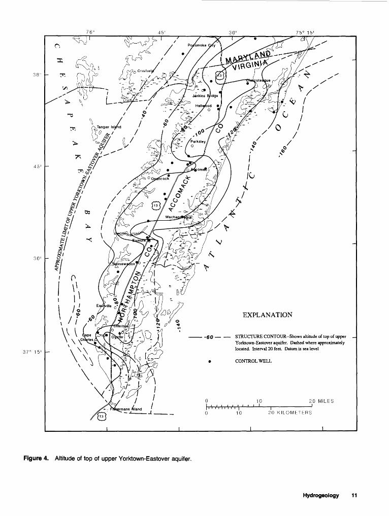
Figure 4. Altitude of top of upper Yorktown-Eastover aquifer.

Hydrogeology 11

76 C 45' 30' 75° 15'

38 C

45'

30'

37° 15'

EXPLANATION

STRUCTURE CONTOUR--Shows altitude of top ofmiddle Yorktown-Eastover confining unit. Dashed where approximately located. Interval 25 feet Datum is sea level

CONTROL WELL

10 20 MILES

20 KILOMETERS

1

Figure 5. Altitude of top of middle Yorktown-Eastover confining unit.


38° -

45' -

30'

37° 15' -

EXPLANATION

.75. STRUCTURE CONTOUR-Shows altitude of top of middle Yorktown-Eastover aquifer. Dashed where approximately located. Interval 25 feet Datum is sea level

CONTROL WELL

0 10.W.M.M- ' ' '

20 MILES

20 KILOMETERS

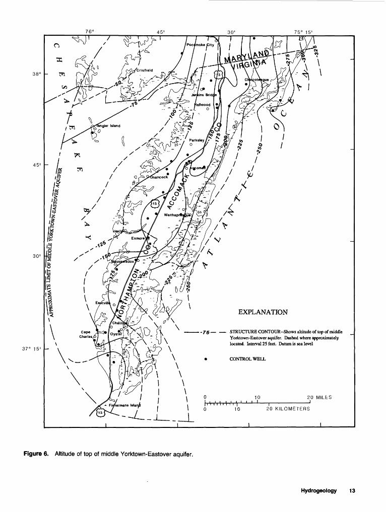
Figure 6. Altitude of top of middle Yorktown-Eastover aquifer.

Hydrogeology 13

76° 45

45

37° 15

EXPLANATION

STRUCTURE CONTOUR--Shows altitude of top of lower Yorktown-Eastover confining unit. Dashed where approximately located. Interval 25 feet. Datum is sea level

20 KILOMETERS

I I

Figure 7. Altitude of top of lower Yorktown-Eastover confining unit.


76°

38° -

45 1 -

-75 STRUCTURE CONTOUR-Shows altitude of top of lower Yorktown-Eastover aquifer. Dashed where approximately located. Interval 25 feet. Datum is sea level

37° 15' -

Figure 8. Altitude of top of lower Yorktown-Eastover aquifer.

Hydrogeology 15

76° 45

EXPLANATION

STRUCTURE CONTOUR-Shows altitude of top of St. Mary confining unit. Dashed where approximately located. Interval 50 feet. Datum is sea level

APPROXIMATE LIMIT ST. MARYS CONFINING

UNIT /

30' -

37" 15' -

Figure 9. Altitude of top of St. Marys confining unit.


WEST

VIRGINIA MAINLAND

EAST

ATLANTIC OCEAN

Y \Upper mktown-Eastover aquifer

e Yorktown-Eastover amufe

Lower Yorktown-Eastover aquife

EASTERN SHORE

$t. Marys-Choptank aquifer

Brightseat aquifer

Middle Pptorhac aquifer

Lower Potbmac aquifer,

^^^NOT TO SCALE

EXPLANATION

GENERALIZED FLOW LINE

FRESHWATER

SALTWATER

CONFINING UNIT

>] BASEMENT ROCKS

Figure 10. Schematic diagram of aquifers and confining units and generalized flow lines.

Hydrogeology 17

Table 2. Statistical summary of transmissivity and storage coefficients derived from aquifer-test results[ft2/d, foot squared per day; , no values reported]

Analytical method

Yorktown-Eastoveraquifer

Nonleaky analysis ofTheis(1935)

Transmissivity (ft 2/d)

Storage coefficient

(dimensionless)

Nonleaky analysis of Cooper and Jacob (1946)

Transmissivity (ft 2/d)

Storage coefficient

(dimensionless)

Upper Maximum

Median Mean Number of

tests

3,960470

1,6701,940

13X10 3 2.0X10" 4 9.7X10" 4

8.6X10" 4

670620

93X10"

4.6X10"

Middle

Lower

MaximumMinimumMedianMeanNumber of

tests

Maximum

MinimumMedianMeanNumber of

tests

2,650230

1,1301,290

4

1,360120

__

2

85X10" 495X10" 5

5.2X10" 44.9X10" 4 350 3.8X10" 4

4 1 1

9.4X10" 42.6X10" *_ _ __ _ _

2

purposes. Irrigation ponds in the Columbia aquifer provide much of the water needed for agricultural purposes. In upland areas, the quality of water in this aquifer is generally within drinking-water stand ards if wells are not located downgradient of poten tial sources of contamination. In low-lying and poorly drained areas, the water quality is worse than in upland areas, reflecting the nearness of saltwater bodies and contamination from land uses.

Pleistocene Paleochannel Aquifers

Evidence indicates the presence of subsurface erosional channels where all or part of the Yorktown Formation sediments have been removed and replaced by marginal-marine deposits of Pleistocene age. The sediments in these paleochannel areas are, therefore, quite different from the Yorktown sedi ments that are typical of the rest of the Eastern Shore. The two major paleochannels that have been identified in the study area cut eastward across the peninsula near Exmore and Eastville, Va. Mixon (1985) describes the lithology of a type cross section in the vicinity of the Eastville paleochannel in

southern Northampton County. The channel is cov ered with a basal-gravelly sand unit that contains pebbles and small cobbles overlain by muddy sand and clay-silt, marginal-marine deposits. The sands and gravels of the channel deposits are extremely transmissive; however, their extent has not yet been defined, and the gravelly sands are overlain by a poorly sorted mixture of mud, silt, and clay of vary ing thicknesses. Detailed study of the paleochannels is necessary to define the extents of the different types of sediments and determine the hydraulic properties associated with those sediments. For the purposes of this report, the channel sediments are hydraulically connected to the surrounding York- town sediments and have been included as part of the Yorktown-Eastover aquifer system.

Yorktown-Eastover Aquifer System

The Yorktown-Eastover aquifer system is a multiaquifer unit consisting of late Miocene and Pli ocene deposits and is composed of the sandy facies of the Yorktown and Eastover Formations (Meng and Harsh, 1988). The Yorktown-Eastover aquifer


Table 3. Statistical summary of well yield, specific capacity, transmissivity, and horizontal hydraulic con ductivity derived from specific-capacity tests[gal/min, gallon per minute; (gal/min)/ft, gallon per minute per foot; ft2/d, foot squared per day; ft/d, foot per day]

Yorktown- Eastover aquifer

Upper

Middle

Lower

Statistic WeU yield

(gal/rain)

MaximumnAnntnntn

MedianMeanNumber of tests

MaximumRfltn iniiini

MedianMeanNumber of tests

MaximumIninimumMedianMeanNumber of tests

3155

120125

14

6452095

13612

2011

345310

Specific capacity

[(gal/min)/ft]

17.52.

1.72.8

14

9.9.7

1.523

12

5.7.1

1.01.8

10

Transmissiviry (ft'/d)

Unadjusted

1.00049

361446

10

912186427487

7

1,69724

209354

Adjusted 1

4^3061

7391,259

10

3,240206834

1,3757

2,09495

353724

4

Horizontal hydraulic conductivity (ft/d)

Unadjusted

17.2.9

1038.9

10

15.63.862837

19.6.4

537.64

Adjusted 1

60.433

10.621310

44342

17.222.7

7

24.21.68.8

10.94

Adjusted for effects of partial penetration.

Table 4. Vertical hydraulic conductivities derived from laboratory analyses of sediment cores from the Jenkins Bridge Research Station[ft/d, foot per day]

Depth of sample below land surface

(feet)

63.7- 64.7 348.7-349.7 368.4-369.4

Vertical hydraulic Confining unit conductivity

(ft/d)

Upper Yorktown-Eastover St Marys St Marys

1.39x10" * 1.63X10" 3

1.27X10" s

system consists of a series of alternating sand and clay-silt units that form three distinct aquifers that generally are present throughout the Eastern Shore. These aquifers are identified as the upper, middle, and lower Yorktown-Eastover aquifers. Correspond ingly, each aquifer is overlain by the upper, middle, and lower Yorktown-Eastover confining units. The entire aquifer system is wedge shaped and thickens and dips eastward. The units extend eastward beneath the Atlantic Ocean to the continental shelf and westward underneath the Chesapeake Bay.

The hydraulic characteristics of the aquifers and confining units determine their ability to store, transmit, and release water. Transmissivity, storage

coefficient, and vertical hydraulic conductivity are the principal hydraulic characteristics necessary for an analysis of ground-water flow. Transmissivities and storage coefficients derived from aquifer-test data for the freshwater-confined aquifers are summa rized in table 2. Few aquifer tests are available that reflect the characteristics of an individual aquifer because most of the wells used for aquifer tests have screens that are open to more than one aquifer. The aquifer-test data are supplemented by transmissivities estimated from specific-capacity data (table 3). Table 3 provides a statistical summary of well yield, specific capacity, transmissivity, and horizontal hydraulic conductivity estimated from specific- capacity tests. A detailed description of the method and equations used to estimate transmissivities from specific-capacity data is presented by Laczniak and Meng (1988). A few point estimates for vertical hydraulic conductivities are available from labora tory analysis of sediment cores from the Jenkins Bridge Research Station (well 66M23) (table 4). These data need to be interpreted and used with cau tion because (1) the core samples could be dis turbed, (2) the core samples represent 1-ft intervals of thicker confining units, and (3) the values are local point values and cannot be interpreted as regional estimates.

Hydrogeology 19

Upper Yorktown-Eastover Aquifer and Confining Unit

The Columbia aquifer is underlain by the upper Yorktown-Eastover confining unit. The con fining unit consists of gray, greenish-gray, or brownish-gray clayey silt or silty clay. The confin ing unit is continuous underneath the peninsula; however, incisement by present-day channels in the Chesapeake Bay has likely removed part or all of the upper Yorktown-Eastover confming-unit sedi ments (figs. 3 and 11) west of the peninsula. In the model area where control wells exist, the confining unit ranges in thickness from 26 ft at well 63F16 in southern Northampton County to 109 ft at well 68M2 on Chincoteague Island. A laboratory analysis of a sediment core from well 66M23 indicates a ver tical hydraulic conductivity of 1.39 x 10~5 ft/d for the upper Yorktown-Eastover confining unit. Analy ses of cores from the St. Marys confining unit, at the same site, indicated similar values (table 4). Elsewhere on the mainland part of the Virginia Coastal Plain, laboratory analyses of confining-unit sediments have ranged from 3.93 x 10~ 3 to 9.2 x 10" 1 ft/d (Harsh and Laczniak, 1986).

The upper Yorktown-Eastover confining unit is underlain by the upper Yorktown-Eastover aquifer (figs. 3,4). Geologic data from the Exmore core (well 64J14) and the VWCB Jenkins Bridge Research Station (well 66M23) indicate that the upper Yorktown-Eastover aquifer predominantly consists of Yorktown Formation (Pliocene) sedi ments. Lithologically, the sediments of the York- town are diverse, consisting of varying mixtures of fine-grained to very coarse-grained, white to greenish-gray, shelly, glauconitic, and pebbly quartz sands (Meng and Harsh, 1988). Hydraulic properties of the upper Yorktown-Eastover aquifer are summa rized in tables 2 and 3. The range of fine-grained to very coarse-grained sediments in the Yorktown For mation and the variable aquifer thickness result in an order of magnitude range in transmissivity val ues. The upper Yorktown-Eastover aquifer extends eastward to the continental shelf and westward underneath the Chesapeake Bay. The characteristics and extent of the upper Yorktown-Eastover aquifer are not known in offshore areas beneath the Atlantic Ocean and the Chesapeake Bay. The upper Yorktown-Eastover aquifer is most likely truncated beneath the Chesapeake Bay by erosion from the ancient Susquehanna River channel and incised by the nearshore channels of the present-day Chesa

peake Bay (Hack, 1957; Colman and others, 1990). In the model area where control wells exist, the upper Yorktown-Eastover aquifer ranges in thickness from 15 ft at well 65L6 in central Accomack County to 110 ft at well 68M4 on Chincoteague Island.

Middle Yorktown-Eastover Aquifer and Confining Unit

The upper Yorktown-Eastover aquifer is underlain by the middle Yorktown-Eastover confin ing unit. The confining unit consists of gray, greenish-gray, or brownish-gray clayey silt or silty clay and ranges in thickness from 8 ft at well 63G24 in southern Northampton County to 76 ft at well MDFC46 in Worcester County, Md. The confining unit is present throughout the study area.

The middle Yorktown-Eastover confining unit is underlain by the middle Yorktown-Eastover aqui fer. Estimated hydraulic properties are summarized in tables 2 and 3. The middle Yorktown-Eastover aquifer consists of sediments from the Yorktown Formation; therefore, the hydraulic properties of the middle Yorktown-Eastover aquifer are similar to those of the upper Yorktown-Eastover aquifer. The middle Yorktown-Eastover aquifer is present throughout the study area. The characteristics and extents of these units in offshore areas are unknown. It is likely that the western limit of the middle Yorktown-Eastover aquifer (fig. 6) extends beyond the western limit of the upper Yorktown-Eastover aquifer (fig. 4) as a result of erosion by the ancient Susquehanna River channel. In the model area, where control wells exist, the middle Yorktown- Eastover aquifer ranges in thickness from 12 ft at well MDCE42 in Somerset County, Md., to 124 ft at well 67N1 in northeastern Accomack County.

Lower Yorktown-Eastover Aquifer and Confining Unit

The middle Yorktown-Eastover aquifer is underlain by the lower Yorktown-Eastover confining unit. The lithology of the confining unit is similar to that of the middle and upper confining units and consists of gray, greenish-gray, or brownish-gray clayey silt or silty clay. The lower Yorktown- Eastover confining unit ranges in thickness from 10 ft at well 62F1 in southern Northampton County to 74 ft at well 68M2 on Chincoteague Island (fig. 2).

The lower Yorktown-Eastover aquifer under lies the lower Yorktown-Eastover confining unit and primarily consists of sediments from the Miocene


60 BATHYMETRIC CONTOUR-Interval, in feet, is variable Datum is sea level

37° 15' -

Figure 11. Bathymetry in the vicinity of the Eastern Shore.

Hydrogeology 21

Eastover Formation. Mixon (1985) describes the Eastover sediments as chiefly fine-grained to very fine-grained, greenish-gray, clayey, silty, and shelly quartz sands. Estimated hydraulic properties of the lower Yorktown-Eastover aquifer are summarized in tables 2 and 3. The Eastover Formation typically contains finer-grained sediments than the Yorktown Formation; therefore, the lower Yorktown-Eastover aquifer generally is less transmissive than the upper and middle Yorktown-Eastover aquifers. The lower Yorktown-Eastover aquifer is present throughout the study area. Because the lower Yorktown-Eastover aquifer is at a greater depth, its limit probably extends farther west underneath the Chesapeake Bay than the middle and upper Yorktown-Eastover aqui fers (figs. 4, 6, and 8). The lower Yorktown- Eastover aquifer ranges in thickness from 22 ft at well 63L1 on Tangier Island (fig. 2) to 140 ft at well 66M23 in Accomack County.

St. Marys Confining Unit

The St. Marys confining unit consists of the predominantly clayey facies of the St. Marys For mation and the lower clayey facies of the Eastover Formation. These sediments are middle to late Mio cene in age. The St. Marys confining unit is con formably overlain throughout the study area by the lower Yorktown-Eastover aquifer. The sediments consist of interbedded silty and sandy clay and vary ing amounts of shells, typically bluish-gray to gray in color (Meng and Harsh, 1988). Laboratory analy ses of sediment cores from the St. Marys confining unit at well 66M23 indicate vertical hydraulic con ductivities of 1.63 x 10~ 5 and 1.27 x 10~ 5 ft/d (table 4). The St. Marys confining unit ranges in thickness from 150 to 350 ft. This massive clay unit is effectively a lower boundary for the fresh ground- water-flow system on the Eastern Shore.

Ground-Water Hydrology

The ground-water-flow system can be divided into a local and a regional ground-water-flow system (fig. 10). The local ground-water-flow system con sists of the unconfined aquifer (Columbia) and the confined-freshwater aquifers (upper, middle, and lower Yorktown-Eastover). The aquifers in the local system contain freshwater that is recharged locally by rainfall on the Eastern Shore and discharges locally to estuaries, marshes, the Chesapeake Bay,

and the Atlantic Ocean. The regional system of the Eastern Shore consists of the confined aquifers beneath the lower Yorktown-Eastover aquifer. Infor mation for these deep confined aquifers beneath the Eastern Shore is limited; however, it is likely that the lower Yorktown-Eastover aquifer is underlain by the St. Marys-Choptank, Brightseat, upper Poto- mac, middle Potomac, and lower Potomac aquifers (Meng and Harsh, 1988). These aquifers are hydraulically separated from the overlying freshwater aqui fers by the thick St. Marys confining unit. The regional aquifers are continuous underneath the Chesapeake Bay, and deep ground-water-flow beneath the Eastern Shore is affected by the regional Coastal Plain ground-water-flow system.

Local Ground-Water-Flow System

A schematic of ground-water flow in the local ground-water system is presented in figure 10. Freshwater recharges the local ground-water system primarily through precipitation that falls on the pen insula and infiltrates into the sediments, because there are no major surface-water bodies on the pen insula. Gushing and others (1973) estimated that 8.5 to 15 in. of the 43 in. of annual precipitation recharges the unconfined aquifer; the remainder is either surface runoff or evaporation. Using an aver age recharge of 12 inches per year (in/yr) over a 450 square mile (mi2) recharge area (total land area minus wetlands) for the Virginia part of the Eastern Shore, the estimated natural recharge to the uncon fined aquifer is 257 Mgal/d. Precipitation infiltrates into the ground and percolates to the water table of the Columbia aquifer. Water in the unconfined aqui fer flows vertically into the lower parts of the unconfined aquifer and laterally through the uncon fined aquifer toward discharge sites such as springs, streams, marshes, estuaries, the Chesapeake Bay, and the Atlantic Ocean. The lateral direction of ground-water flow generally is from the ground- water divide at the center of the peninsula to the Chesapeake Bay and Atlantic Ocean. Eventually, water that is moving vertically encounters the upper Yorktown-Eastover confining unit, and much of the flow is forced to move laterally through the uncon fined aquifer. Under natural (prepumping) condi tions, a comparatively small amount of water is able to flow through the less permeable confining unit into the confined-aquifer system. The predominant movement of ground water is in a lateral direction


through aquifers and in a vertical direction through confining units. Where fresh ground water encoun ters salty ground water, the less dense freshwater is forced upward. The upward-moving fresh ground water is again inhibited by confining units but even tually discharges into marshes, estuaries, the bay, and ocean.

Water levels in wells in the Columbia aquifer indicate the direction of ground-water flow and the response of the system to recharge and discharge. Well-construction information for wells along a transect from the topographic high (ground-water divide) near U.S. Route 13 near Townsend, Va., to the marsh adjacent to Magothy Bay (ground-water- discharge area) (fig. 12) is presented in table 5. Water levels fluctuate throughout the year in response to the amount of recharge to and discharge from the system (fig. 13). Water-level declines in this agricultural area during the spring and summer indicate the effects of increased evapotranspiration. Water levels are highest at well 63F31 near the cen ter of the peninsula and decline toward the coast (fig. 13). The water-level gradients indicate that ground water flows from the topographic high in the center of the peninsula to the lowlands adjacent to Magothy Bay. Water levels from an irrigation pond (63F38) and a nearby well (63F31) show the response of the unconfined aquifer to pumping (fig. 14). The water level in well 63F31 shows little response to the greater than 4-ft decline in water levels in the pond caused by pumpage during the 1989 growing season. Pumpage from the irrigation pond only has a local effect on ground-water levels because of the high permeability of the coarse grained sediments in the unconfined aquifer.

Temporal water-level trends and vertical gradi ents in water levels provide additional information about the response of the ground-water-flow system to recharge, discharge, and pumpage stress. The VWCB has constructed a series of research stations on the Eastern Shore to monitor such responses (fig. 15). Each research station consists of a cluster of wells with individual wells screened in different aquifers. Well identifiers, well location, and well- construction information for wells in selected research stations are summarized in table 6. Water levels from research-station wells provide informa tion about the vertical direction of flow between aquifers. Water levels for two research stations on the Eastern Shore that illustrate the vertical direc tions of flow in this multiaquifer system are shown

Table 5. Well-construction data for wells completed in the Columbia aquifer in a transect A-A' near Townsend, Va.[Datum is sea level; well depth is in feet below land surface datum; USGS, U.S. Geological Survey]

USGS weU number

63F2563F2663F2763F2963F3063F3163F3263F3863F49

Station number

371145075565901371143075565801371133075570401371121075565001371128075572101371136075580201371136075574801371144075580201371125075570205

Land-surface elevation (feet)

1238153722.9213.4029.0331.79285522.002735

WeU depth (feet)

6.68.9

12.79.5

15.012.012.0

pond16.8

in figure 16. The water levels for the research sta tion in a recharge area (fig. 16A) reflect downward vertical flow from the unconfined aquifer (well 64K10), to the upper Yorktown-Eastover aquifer (well 64K11), to the lower Yorktown-Eastover aqui fer (well 64K12). In contrast, the water levels pre sented in figure 16B indicate upward flow in a coastal discharge area. Well 64J11 is screened in the lower Yorktown-Eastover aquifer, whereas wells 64J10 and 64J9 are screened in the middle and upper Yorktown-Eastover aquifers, respectively. Except for the early period of record when water levels appear to be affected by pumping, heads in the wells for this research station reflect vertical flow in an upward direction as ground water flows toward discharge sites in the coastal marshes, estu aries, and ocean.

Regional Ground-Water-Flow System

The regional ground-water-flow system con sists of the confined aquifers beneath the lower Yorktown-Eastover aquifer (fig. 10). These aquifers are continuous underneath the Chesapeake Bay and are part of the westward-thinning wedge of unconsolidated sediments that make up the Coastal Plain of Virginia. Ground-water flow in these deep con fined aquifers beneath the Eastern Shore is affected by the Chesapeake Bay and regional ground-water flow from the Virginia mainland. Freshwater is recharged to the deep confined aquifers from precip itation that falls on the Virginia mainland and infil trates into the confined system. At the northern end of the peninsula, fresh ground water flows farther beneath the Chesapeake Bay and the Eastern Shore

Hydrogeology 23

CO

NTO

UR

IN

TER

VA

L 5

FEE

T N

ATI

ON

AL

GE

OD

ETI

C V

ER

TIC

AL

DA

TUM

OF

1929

EX

PL

AN

AT

ION

^63

F31

WE

LL A

ND

Figu

re 1

2.

Loca

tions

of w

ells

alo

ng t

rans

ect A

-A'

in t

he C

olum

bia

aqui

fer.

UJ>UJ

UJ CO

HI

oCO

UJ UJu.

UJ>UJ_JDC UJ

27

26

25

24

23

22

21

20

19

18

17

16

15

14

13

12

11

10

9

8SONDJFMAMJJ ASONDJFMAMJJASONDJFMAMJ JASOND

1987 1988 1989 1990

Figure 13. Water levels in selected wells along transect A-A' in the Columbia aquifer.

than at the southern end. The northern end of the peninsula is closer to higher landmasses; therefore, it has a nearby freshwater source. The freshwater heads at the southern part of the Virginia Coastal Plain are not high enough to force the saltwater out of the deep sediments beneath the Chesapeake Bay and Eastern Shore.

Chloride concentrations support this conceptu alization of ground-water flow. Chloride concentra tions in ground water from the upper Potomac aqui fer for the Virginia Coastal Plain are lower along the coast in the northeastern part of the Virginia mainland than in the southeastern part (fig. 17). The chloride concentration is 150 mg/L in water from well 63L4 on Tangier Island, which is screened in the upper Potomac aquifer. Chloride concentrations

in water from wells at approximately the same lon gitude in the southeastern part of the Virginia main land range from 1,360 to 1,900 mg/L in the upper Potomac aquifer. Research-station well clusters on the Eastern Shore also indicate a stronger regional freshwater influence in the northern part of the East ern Shore than in the southern part. The vertical chloride distribution is shown in table 7 for the two research-station well clusters on the Eastern Shore that have wells located in the upper Potomac aqui fer. At the Jenkins Bridge Research Station, chlo ride concentrations are lower in the upper Potomac aquifer (1,500 mg/L) than in the overlying St. Marys-Choptank (3,800 mg/L) and lower Yorktown-Eastover (2,100 mg/L) aquifers. The ver tical profile of chloride concentrations from the

Hydrogeology 25

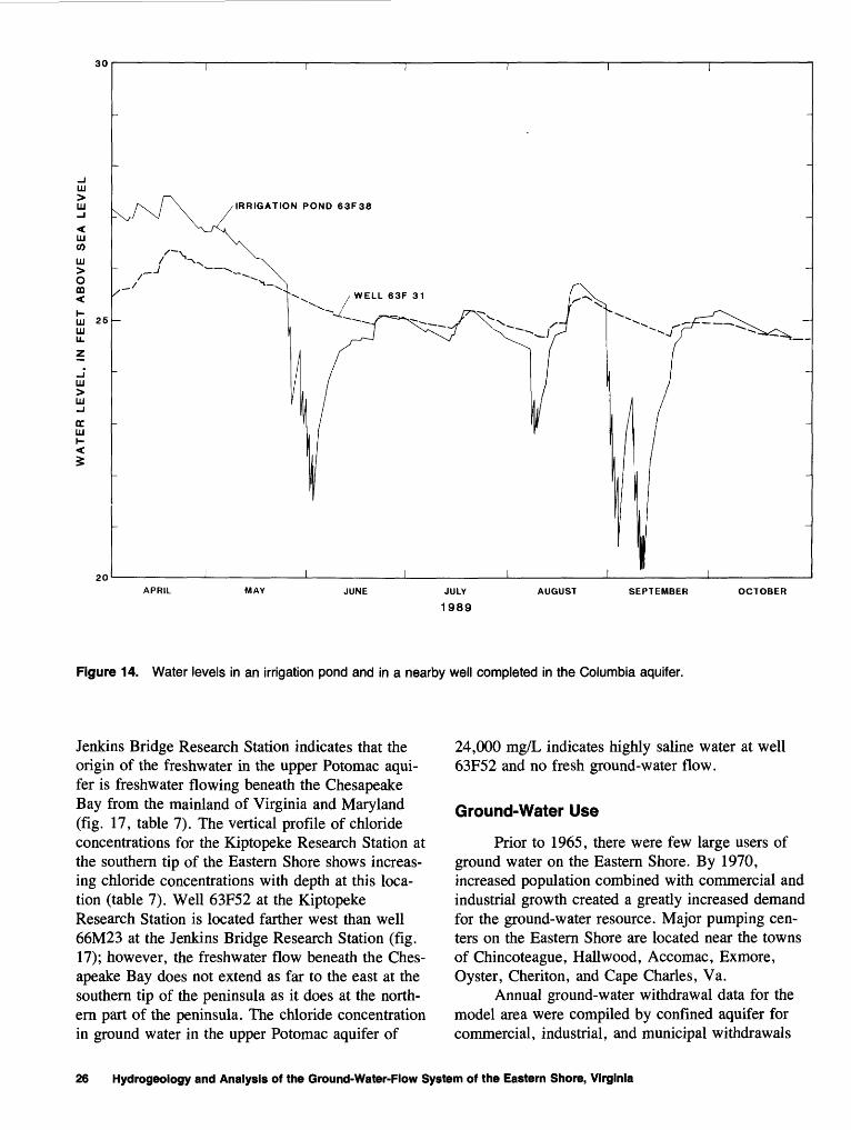
30

LU CO

LU>oCO

UJ 25 LU

20

IRRIGATION POND 63F38

APRIL MAY JUNE JULY

1989

AUGUST SEPTEMBER OCTOBER

Figure 14. Water levels in an irrigation pond and in a nearby well completed in the Columbia aquifer.

Jenkins Bridge Research Station indicates that the origin of the freshwater in the upper Potomac aqui fer is freshwater flowing beneath the Chesapeake Bay from the mainland of Virginia and Maryland (fig. 17, table 7). The vertical profile of chloride concentrations for the Kiptopeke Research Station at the southern tip of the Eastern Shore shows increas ing chloride concentrations with depth at this loca tion (table 7). Well 63F52 at the Kiptopeke Research Station is located farther west than well 66M23 at the Jenkins Bridge Research Station (fig. 17); however, the freshwater flow beneath the Ches apeake Bay does not extend as far to the east at the southern tip of the peninsula as it does at the north ern part of the peninsula. The chloride concentration in ground water in the upper Potomac aquifer of

24,000 mg/L indicates highly saline water at well 63F52 and no fresh ground-water flow.

Ground-Water Use

Prior to 1965, there were few large users of ground water on the Eastern Shore. By 1970, increased population combined with commercial and industrial growth created a greatly increased demand for the ground-water resource. Major pumping cen ters on the Eastern Shore are located near the towns of Chincoteague, Hall wood, Accomac, Exmore, Oyster, Cheriton, and Cape Charles, Va.

Annual ground-water withdrawal data for the model area were compiled by confined aquifer for commercial, industrial, and municipal withdrawals


38° -

45' -

30' -

37° 15' -

67M10 i67M11 Chiricoteague67M12 -* ^ ^67M1367M14

65K27 Tangier Island 65K2e0 65K29

65K30

Cape63F15 Chartoi 63F16 63F17

EXPLANATION

RESEARCH STATION AND WELL IDENTIFICATION

20 MILES i

20 KILOMETERS

Figure 15. Location of selected Virginia Water Control Board research-station well clusters.

Hydrogeology 27

Table 6. Selected Virginia Water Control Board research-station well clusters on the Eastern Shore[Latitude and longitude are reported in degrees, arc minutes, and arc seconds; USGS, U.S. Geological Survey; VWCB, Virginia Water Control Board]

USGS well number

66K466K366K264H664H7

64H563H663H563H463G21

63G1763G1663G1S63F1563F17

63F1664K964K864K766L2

66L366L164K1064K1164K12

65K2665K2465K2565K2366M19

66M1666M1766M1863G2563G22

63G2363G2464J1264J964J10

64J11631163J263J365K30

VWCB wen number

SOW 101ASOW 101BSOW 101CSOW102ASOW102B

SOW 102CSOW 103ASOW 103BSOW 103CSOW104S

SOW 104ASOW 104BSOW104CSOW105ASOW 105B

SOW 105CSOW106ASOW106BSOW106CSOW 107A

SOW107BSOW 107CSOW 108ASOW 108BSOW 108C

SOW109SSOW 109ASOW 109BSOW109CSOW110S

SOW110Asow HOBsow iiocSOW 11 ISSOW111A

SOW 11 IBSOW 11 1CSOW112SSOW112ASOW112B

SOW112CSOW113ASOW113BSOW113CSOW114S

Latitude

374320374320374319372925372921

372921372705372705372706371709

371709371709371709371307371307

371307373845373845373845375225

375225375225373932373932373932

374442374442374442374428375723

375723375723375723371653371653

371653371653373059373059373059

373059373216373216373216374425

Longitude

07536560753805075365407547040754705

07547050755559075555907555590755608

07556080755608075560707558350755835

07558350755225075522507552250753217

07532170753217075452707545270754527

07543250754325075432507543280753444

07534440753444075344507558480755848

07558480755848075484507548450754845

07548450755407075540707554070754000

Wen depth (feet)

152220292154220

30637

13223536

140240310130196

2853795

176140

20630550

180284

2513022829036

13017824070

150

280330

47135210

31312022529040

Aquifer penetrated

Upper Yorktown-EastoverMiddle Yorktown-EastoverLower Yorktown-EastoverUpper Yorictown-EastoverMiddle Yorktown-Eastover

Lower Yorktown-EastoverColumbiaUpper Yorktown-EastoverLower Yorktown-EastoverColumbia

Upper Yorktown-EastoverMiddle Yorktown-EastoverLower Yorktown-EastoverUpper Yorktown-EastoverMiddle Yorktown-Eastover

Lower Yorktown-EastoverColumbiaUpper Yorktown-EastoverLower Yorktown-EastoverUpper Yorktown-Eastover

Middle Yorktown-EastoverLower Yorktown-EastoverColumbiaUpper Yorktown-EastoverLower Yorktown-Eastover

ColumbiaUpper Yorktown-EastoverLower Yorktown-EastoverLower Yorktown-EastoverColumbia

Upper Yorktown-EastoverMiddle Yorktown-EastoverLower Yorktown-EastoverColumbiaUpper Yorktown-Eastover

Lower Yorktown-EastoverLower Yorktown-EastoverColumbiaUpper Yorktown-EastoverMiddle Yorktown-Eastover

Lower Yorktown-EastoverUpper Yorktown-EastoverMiddle Yorktown-EastoverLower Yorktown-EastoverColumbia


Table 6. Selected Virginia Water Control Board research-station well clusters on the Eastern Shore- Continued

usesweU number

65K276SK2865K2967M1067M11

67M1267M1367M1466M2366M24

66M2566M2666M2763F5163F52

63F5363F5463F55

VWCB well number

SOW114ASOW114BSOW114CSOW 1 ISASOW115B

SOW115CSOW115DSOW115ESOW 181ASOW 18 IB

SOW 181CSOW 18 IDSOW 18 IESOW 182ASOW182B

SOW182CSOW 182DSOW 182E

Latitude

374425374425374427375635375635

375635375635375617375610375610

375610375610375610370807370807

370807370807370807

Longitude

07540000754000075400007527150752715

0752715075271507527370753618075 36 18

07536180753618075361807557080755708

075570807557080755708

Wen depth (feet)

160230315

52138

222249280

1,300508

34023030

1,7301,332

2206020

Aquifer penetrated

Upper Yoiktown-EastoverMiddle Yoiktown-EastoverLower Yoiktown-EastoverColumbiaUpper Yoiktown-Eastover

Middle Yoiktown-EastoverMiddle Yoiktown-EastoverMiddle Yoiktown-EastoverUpper PotomacSt. Marys

Lower Yoiktown-EastoverLower Yoiktown-EastoverColumbiaMiddle PotomacUpper Potomac

Lower Yoiktown-EastoverUpper Yoiktown-EastoverColumbia

Table 7. Vertical distribution of chloride concentrations in ground water at Jenkins Bridge and Kip- topeke Research Station well clusters[USGS, U.S. Geological Survey; mg/L, milligrams per liter]

USGS weU number

66M27

66M26

66M25

66M24

66M25

63F5563F5463F5363F52

WeU depth (feet)

40

230

340

508

1^20

2060

2201,332

Aquifer

Jenkins Bridge Research Station

Columbia

Lower Yorktown-Eastover

Lower Yorktown-Eastover

St. Marys - Choptank

Upper Potomac

Kiptopeke Research Station

ColumbiaUpper Yorktown-EastoverLower Yorktown-EastoverUpper Potomac

Date

10-29-8708-29-8810-30-8708-29-8810-30-8708-29-8810-28-8708-29-8810-29-8708-29-88

11-16-8911-16-8911-16-8911-29-89

Chloride concentration

(mg/L)

3123

1,000810

2,1002.1003,9003.8001,5001,500

243259

24,000

Hydrogeology 29

55

LU >LU_l

5 45 COUJ

oCO

35

LU

U-J25

QCLU

I15

I I I I I I

10

\ 64K12

A/\

1978 1979 1980 1981 1982 1983 1984 1985 1986 1987 1988 1989

BLU

LU

10

< a LU 8CO

g eLUm

LU

SmLU oLU

-2

LU

QC LUS-6

1979 1980 1981 1982 1983 1984 1985 1986 1987 1988 1989

Figure 16. Water levels in research-station well clusters (A) in a recharge area and (B) in a discharge area.


77' 76°

38"

37"

EXPLANATION

OBSERVATION WELL-Upper number is

well identifier Lower number is

chloride concentration in milligrams

per liter

20 MILES

Figure 17. Location of observation wells and chloride concentrations in the upper Potomac aquifer for the Coastal Plain of Virginia.

Hydrogeology 31

DC HI 0.

eoz o

z o

EXPLANATION

UPPER YORKTOWN-EASTOVER AQUIFER

MIDDLE YORKTOWN-EASTOVER AQUIFER

LOWER YORKTOWN-EASTOVER AQUIFER

TOTAL

DC OII-

1945 1950 1955 1960 1965 1970 1975 1980 1985 1990

Figure 18. Annual ground-water withdrawal from model area.

(fig. 18). Estimates do not include domestic or agri cultural withdrawals. Domestic use is not included because currently there is no practical method of collecting such data by aquifer, and it is assumed to represent only a small percentage of nonreturned water. Agricultural use is significant on the Eastern Shore; however, agricultural users are not required to report withdrawals. As a result, the specific loca tions and aquifers tapped for agricultural withdraw als are unknown. Most of the ground water used for agricultural purposes is withdrawn from irrigation ponds in the unconfined Columbia aquifer. All other ground-water users in Northampton and Accomack Counties that withdraw over 300,000 gal/month are required to report usage data to the VWCB. The depth of the well screen was used to determine the

aquifer from which water was pumped. For wells screened in multiple aquifers, water-withdrawal rates from each aquifer were estimated from the ratio of the length of screen in each aquifer to the total length of well screen.

The middle and upper Yorktown-Eastover aquifers have historically provided most of the freshwater to users on the Eastern Shore. Prior to 1968, the largest withdrawals were from the shal lowest confined aquifer, the upper Yorktown- Eastover. By 1970, the middle Yorktown-Eastover aquifer was contributing more water than the upper or lower Yorktown-Eastover aquifers, and pumpage from the lower Yorktown-Eastover aquifer was increasing. Estimated ground-water use peaked in 1974 at 6.96 Mgal/d. The decline in water use for


the period 1975-83 represents the loss of several major industrial users. Since 1985, water use has generally been steady. Total ground-water use was estimated to be about 5.04 Mgal/d in 1988. The upper Yorktown-Eastover aquifer supplied 36 per cent of the withdrawal in 1988, and the middle and lower Yorktown-Eastover aquifers supplied 42 and 22 percent, respectively.

Chloride Distribution

Chloride concentrations were compiled by aquifer to provide information on the distribution of chlorides in the aquifers that currently are being used as a freshwater supply for the Eastern Shore (figs. 19-22). The chloride concentrations presented on the maps are the most recent chloride analyses for each well. Individual chloride analyses are pre sented by aquifer in tables 8-11. Chloride concen trations typically are greater along the coast than in the center of the peninsula. Chloride concentrations in water collected from wells in the Columbia aqui fer and the upper Yorktown-Eastover aquifer were less than the U.S. Environmental Protection Agency (USEPA) secondary drinking-water regulation of 250 mg/L (U.S. Environmental Protection Agency, 1989). The line delineating the approximate limit of the 250 mg/L chloride concentration in the Colum bia aquifer was estimated to be the landward limit of the saltwater marshes and estuaries (fig. 19). All chlorides from the upper Yorktown-Eastover aquifer were well below the 250 mg/L limit; therefore, the limit line was estimated based on the understanding of the ground-water-flow system (fig. 20). Chloride concentrations probably are less than 250 mg/L in the upper Yorktown-Eastover aquifer beneath all major land surfaces on the peninsula. Chloride con centrations generally increase with depth; greater chloride concentrations are found in the lower Yorktown-Eastover aquifer than in the overlying middle Yorktown-Eastover, upper Yorktown- Eastover, and Columbia aquifers. Chloride concen trations in water in the lower Yorktown-Eastover aquifer are stratified; concentrations are less near the top of the aquifer than near the bottom of the aqui fer. Data indicate an area of elevated chloride con centrations in water in the middle and lower Yorktown-Eastover aquifer near Exmore, Va. (figs. 21, 22). The elevated concentrations appear to be in the area of an ancient Pleistocene river chan

nel (described in Pleistocene Paleochannel Aquifers section). The erosion of the original aquifer and confining-unit materials combined with the different hydraulic characteristics of the backfilled-channel sediments could result in a better hydraulic connec tion between the freshwater-flow system and the saltwater-flow system in this area. A detailed study of the extent of the erosion and the hydraulic prop erties of the channel-fill sediments is needed for a complete understanding of saltwater-freshwater rela tions in this part of the ground-water-flow system. Elevated chloride concentrations in water in the middle and lower Yorktown-Eastover aquifers also are present near Cape Charles, Va. This area could be affected by the southernmost paleochannel or by incision from a nearshore channel in the present-day Chesapeake Bay.

ANALYSIS OF THE GROUND-WATER- FLOW SYSTEM

The conceptualization of the physical charac teristics of the three-dimensional, multiaquifer, flow system can be incorporated into a digital ground- water-flow model. The model is a mathematical rep resentation of the natural system and includes many simplifying assumptions. Model input parameters are based on the measured and estimated character istics of the aquifers and confining units. The model is calibrated by comparing simulated water levels to water levels measured at observation wells. Once calibrated, the digital model can be used within its limitations to simulate changes in ground-water-flow conditions that result from changes in hydrologic stresses. A digital model can assist in analyzing a ground-water system; however, it is important to realize that the model is only an approximate repre sentation of the actual physical system.

Development of the Flow Model

A ground-water-flow model was developed for the Eastern Shore using SHARP (Essaid, 1990a), a numerical finite-difference model that uses a quasi- three-dimensional approach to simulate freshwater and saltwater flow separated by a sharp interface. The sharp-interface approach assumes that saltwater- between saltwater and freshwater is small relative to the thickness of the aquifer. The approach does not provide information on the physical or chemical

Analysis of the Ground-Water-Flow System 33

76 C 45' 30' 75° 15'

38°

45'

30'

37° 15'

EXPLANATION

CHLORIDE CONCENTRATIONS LESS THAN 250 MILLIGRAMS PER LITER

__ __ APPROXIMATE LIMIT OF 250 MILLIGRAMS PER LITER CHLORIDE CONCENTRATION

23 WELL Number is chloride concentration in milligrams per liter

20 MILES

20 KILOMETERS

Figure 19. Chloride concentrations in the Columbia aquifer.


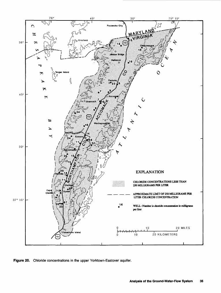
76 C 45' 30' 75° 15'

38 C

45'

30'

37° 15'

o

a:

w

EXPLANATION


APPROXIMATE LIMIT OF 250 MILLIGRAMS PER LITER CHLORIDE CONCENTRATION

WELL-Number it chloride concentration in milligrams per liter

10 20 MILES

10 20 KILOMETERS

Figure 20. Chloride concentrations in the upper Yorktown-Eastover aquifer.


75° 15'

EXPLANATION


__ __ __ APPROXIMATE UMTT OF 250 MILLIGRAMS PER LITER CHLORIDE CONCENTRATION

18J° WELL-Number it chloride concentration in milUgnnuper liter

37° 15' -

Figure 21. Chloride concentrations in the middle Yorktown-Eastover aquifer.


76' 45' 30' 75° 15'

38'

45'

3D 1

37° 15'

EXPLANATION

WELL Number is chloride concentration in milligrams per liter

20 MILES

20 KILOMETERS

Figure 22. Chloride concentrations in the lower Yorktown-Eastover aquifer.


Table 8. Chloride concentrations in the Columbia aquifer[USGS, U.S. Geological Survey; VWCB, Virginia Water Control Board; latitude and longitude are reported in degrees, arc minutes, arc seconds; mg/L, milligrams per liter]

USGS well number

62F 463F 663F1963F2063F21

63F22

63G21

63G2S

63H.6

631 464J12

64J26

64K9

64K10

65K2165K2665K30

65K3265K3366M19

66M2166M27

67M667M10

Latitude

371456370806370806370806370806

370939

371709

371653

372705

373220373059

373200

373845

373932

374257374442374425

374232374249375723

375403375610

375624375635

Longitude

07600300755718075570907557080755707

0755704

0755608

0755848

0755559

07554150754845

0754917

0755225

0754527

075404107543250754000

075434207542070753444

07530250753618

07528360752715

WeU depth (feet)

4074606265

46

36

70

37

4047

58

37

50

452540

525536

6930

4552

Land- surface altitude (feet)

1010101010

10

30

15

17

2530

35

2

45

421045

304010

355

3015

Chloride concentration (mg/L)

735423263132322736664332131543302322231841

105927892

3636

189

1912211915151638312310141216

Date sampled

12-01-7709-27-5501-02-7501-02-7501-02-7502-12-7512-12-7501-02-7512-12-7510-03-7708-19-8008-04-8606-29-7908-19-8009-28-7705-11-7906-26-8405-11-8407-03-7908-21-8003-01-6704-01-7509-19-7809-21-7708-20-8006-26-8408-20-8006-29-8409-28-7108-20-8002-13-8008-26-8008-07-8108-07-8108-26-8007-11-8408-04-8110-29-8708-29-8808-17-4808-13-8105-27-8208-13-84

Sampling agency

VWCBUSGSVWCBVWCBVWCBVWCBVWCBVWCBVWCBVWCBVWCBVWCBVWCBVWCBVWCBVWCBVWCBVWCBVWCBVWCBVWCBVWCBVWCBVWCBVWCBVWCBVWCBVWCBVWCBVWCBVWCBVWCBVWCBVWCBVWCBVWCBVWCBUSGSUSGSVWCBVWCBVWCBVWCB

nature of the transition zone; however, it does repre sent the overall ground-water flow in the system and will reproduce the general response of the interface to applied stresses (Essaid, 1986). The model repre sents regional-scale ground-water-flow systems as a layered sequence of two-dimensional aquifers sepa

rated by confining units that are represented by a vertical leakance term. Vertical gradients within aquifers are not represented; therefore, the modeling approach is not fully three-dimensional. The quasi- three-dimensional solution of the ground-water-flow equation requires several assumptions: (1) flow in


the aquifers is in the lateral direction, (2) vertical flow is controlled by confining units, and (3) water released from confming-unit storage is negligible. These assumptions are considered valid when the lateral and vertical hydraulic conductivities of the aquifers are much greater than those of the confin ing units, and simulation times are long enough to minimize the effects of water released from confining-unit storage.

The Eastern Shore is a peninsula surrounded by saltwater; therefore, the model's inclusion of saltwater-flow dynamics is of particular importance to an analysis of the ground- water system. Any change in offshore freshwater discharge induces movement of the interface between freshwater and saltwater. The rate of interface movement is a func tion of the flow conditions and aquifer properties of the freshwater and saltwater flow domains.

The model uses two vertically integrated, par abolic, partial-differential flow equations, represent ing freshwater and saltwater flow, which must be simultaneously solved for freshwater and saltwater head, as follows (Essaid, 1986):

at at

dd><T J

at

and

where Kfa, Ksx =the freshwater and saltwater hydraulic

conductivities in the x direction (L7"" 1 ); Kfy, Ksy =ihe freshwater and saltwater hydraulic

conductivities in the v direction (LT l)\ Qf-> Gj = the freshwater and saltwater source/sink

terms (LT~ l ); Qy, <2/.y=the freshwater and saltwater leakage

terms (LT 1 ), calculated using Darcy's law;

Bp Bs =the thicknesses of the freshwater and salt water zones (L);

Sf, Ss =the freshwater and saltwater specific stor

ages (L *);cf>y, fys = freshwater and saltwater heads (L);

n= effective porosity; f=time (7); and

a=a parameter equal to 1 for unconfinedaquifers and zero for confined aquifers.

The flow equations for the freshwater and salt water zones are coupled by the interface boundary condition. Continuity of flux and pressure must be maintained at the interface; the fluid pressure of the freshwater must equal the fluid pressure of the salt water (Bear, 1979).

(3)

wherePp Ps = *he freshwater and saltwater fluid pres

sures (ML-1r~2); fy, ^=the freshwater and saltwater specific

weights (MZT 2r~2); and £/=the interface elevation (L).

Solving for the interface elevation,

(4)

where 8=-y//('yJ y/).Once the freshwater and saltwater heads have

been obtained from equations 1 and 2, the interface elevation can be calculated from equation 4.

The SHARP model calculates and tracks the positions of the interface tip and toe in the finite- difference grid for each aquifer. The interface tip is the intersection of the interface with the top of the aquifer, and the interface toe is the intersection of the interface with the bottom of the aquifer (fig. 23). The interface position will not always coincide with the grid block boundaries. The tip and toe are located by linearly projecting the interface, based on the interface elevations at grid points. On the freshwater side of the interface toe, the entire thickness of the aquifer contains freshwater. Simi larly, on the saltwater side of the interface tip, the entire thickness of the aquifer contains saltwater. In the area between the interface tip and toe, the aqui fer contains freshwater and saltwater.

The sharp-interface approach assumes that saltwater and freshwater do not mix. Vertical leak age between saltwater and freshwater is restricted. Saltwater is not allowed to leak into the freshwater zone, and freshwater is not allowed to leak down ward into the saltwater zone. A node can contain


Table 9. Chloride concentrations in the upper Yorktown-Eastover aquifer[USGS, U.S. Geological Survey; VWCB, Virginia Water Control Board; latitude and longitude are reported in degrees, arc minutes, arc seconds; mg/L, milligrams per liter]

USGS well number

62F363F15

63F1863F2463G963G17

63G22

63G37

63H5

63H1063H1163 Jl

64H6

64 J 2

64 J 9

64J18

64J24

Latitude

371456371307

37 13 12371302372134371709

371653

372106

372705

372412372608373230

372905

372235

373059

373503

373045

Longitude

07600270755835

0755915075580707559080755608

0755848

0755620

0755559

075 54 150755307075 54 10

0754740

0755335

0754845

0754920

0754829

Well depth (feet)

130130

112140134140

150

165

132

152180120

154

190

135

167

130

Land- surfacegUtitnde

(feet)

1231

15372

28

15

38

17

383022

6

34

30

31

7


820252518672016242419886

17141315131215151417361614242424283515152724524951141514111213101048

Date sampled

02-01-7706-07-7808-11-8007-12-8404-05-8001-08-8105-26-5410-03-7708-18-8008-06-8402-28-8906-29-7908-19-8007-12-8411-01-7411-28-7802-26-7905-02-7908-20-7912-06-7901-28-8008-28-8002-19-8108-24-8107-21-8206-16-8307-23-8409-28-7705-11-7906-26-8401-25-8803-02-8912-18-8012-18-8008-25-8006-28-8406-01-7707-11-8403-01-8910-27-6901-29-7002-18-7507-03-7908-22-8002-01-7508-01-7802-19-8108-02-79

SflTTlTlllflg

agency

VWCBVWCBVWCBVWCBVWCBUSGSVWCBVWCBVWCBVWCBUSGSVWCBVWCBVWCBVWCBVWCBVWCBVWCBVWCBVWCBVWCBVWCBVWCBVWCBVWCBVWCBVWCBVWCBVWCBVWCBUSGSUSGSVWCBVWCBVWCBVWCBVWCBVWCBUSGSUSGSUSGSVWCBVWCBVWCBVWCBVWCBVWCBVWCB


Table 9. Chloride concentrations in the upper Yorktown-Eastover aquifer Continued

USGS wen number

64K8

64K11

6SK6

6SK9

6SK22

65K2465K27

65L3

66K4

66L2

66L466M16

66M2267M11

Latitude

373845

373932

373830

374233

37 41 53

374442374425

373730

374320

375225

374625375723

375920375635

Longitude

0755225

075 45 27

0754000

0754432

0754309

07543250754000

0754000

0753656

0753217

07536460753444

07532050752715

Wefl depth (feet)

95

180

190

159

180

130160

160

152

140

160130

132138


3

47

43

17

43

1245

40

10

5

4011

2114


334147341098

10101098885

104977

1097

242420222223

88689

13141528231919

Date sampled

09-21-7708-20-8006-26-8403-02-8908-20-8006-29-8401-26-8810-21-7103-04-7202-26-7509-10-7509-28-7103-06-8002-19-8108-24-8102-11-8209-28-8203-29-8411-19-8408-13-8002-13-8007-09-8404-22-6001-05-7203-07-7206-01-7206-27-7711-14-7702-23-78OSO3-7707-10-8409-21-7707-10-8408-04-8108-26-8007-11-8403-30-8203-29-8105-12-8105-27-8208-07-84

SfJtnpliTig

agency

VWCBVWCBVWCBUSGSVWCBVWCBUSGSUSGSUSGSVWCBUSGSUSGSVWCBVWCBVWCBVWCBVWCBVWCBVWCBVWCBVWCBVWCBVWCBUSGSUSGSVWCBVWCBVWCBVWCBVWCBVWCBVWCBVWCBVWCBVWCBVWCBVWCBVWCBVWCBVWCBVWCB

freshwater, saltwater, or both freshwater and salt water. Upward freshwater leakage is distributed between the saltwater and freshwater zones based on the volume of each type of water in the node receiv ing the leakage. If freshwater is leaking upward into a node that contains 80-percent freshwater and 20-percent saltwater, then 80 percent of the leakage will be incorporated into the freshwater zone and 20 percent of the leakage will be incorporated into the saltwater zone. If freshwater is leaking upward into

a node that contains all saltwater, then all the fresh water leakage will be incorporated into the saltwater zone (Essaid, 1990a). Vertical leakage of saltwater into freshwater is not directly simulated; evidence of vertical saltwater intrusion is provided by examina tion of the hydraulic gradients and areas of reversed ground-water flow.

The sharp-interface modeling approach neglects hydrodynamic dispersion; therefore, the interface position does not represent a particular


Table 10. Chloride concentrations in the middle Yorktown-Eastover aquifer[USGS, U.S. Geological Survey; VWCB, Virginia Water Control Board; latitude and longitude are reported in degrees, arc minutes, arc seconds; mg/L, milligrams per liter]

USGS weH number

62F 262G 462G 862G 962G1562G16

63F10

63F17

63G16

63G2763G34

63G35

63G36

63G4363J264H7

64H 964J 7

64J10

64J1764J21

64J2364K3

Latitude

37145637225037154037 15 39371543371544

371057

371307

371709

37 17 1037 17 15

37 17 15

37 17 11

371620373230372905

372830372245

373059

373507373159

373146373756

Longitude

076003007553350760121076011407600340760118

0755814

0755835

0755608

07555220755521

0755521

0755524

075581507554100754740

07551320755335

0754845

07551550754915

07550470754906

Well depth (feet)

210210200170190221

220

196

240

185186

186

185

215225220

245228

210

180229

190210


121212121212

27

31

28

53

5

6

15226

3734

30

3035

2825


1224

170250175114130121124144129161147171

1415131172203115141418191517251719161511

1.400400340400430350

101715121536353510

20841531012

Date sampled

12-01-7701-04-7210-17-7510-17-7508-06-8405-09-7708-01-7711-28-7801-28-8002-19-8107-22-8202-28-8301-23-8405-15-8509-11-7502-01-7508-01-8007-12-8410-03-7708-18-7909-26-7908-06-8401-25-8802-28-8908-25-8009-23-8107-22-8203-14-8304-07-7510-16-8102-12-7504-01-7503-26-8003-03-8908-06-8606-01-7707-11-8408-05-8611-12-8703-01-8905-11-8406-02-6509-10-7012-19-7211-12-7407-03-7908-21-8002-22-8808-07-8103-01-6709-19-7808-01-7908-31-8112-31-06

Sampling agency

USGSUSGSUSGSVWCBVWCBVWCBVWCBVWCBVWCBVWCBVWCBVWCBVWCBVWCBUSGSVWCBVWCBVWCBVWCBVWCBVWCBVWCBUSGSUSGSVWCBVWCBVWCBVWCBVWCBVWCBVWCBVWCBVWCBVWCBVWCBVWCBVWCBVWCBUSGSUSGSVWCBVWCBVWCBVWCBVWCBVWCBVWCBUSGSVWCBVWCBVWCBVWCBVWCBUSGS


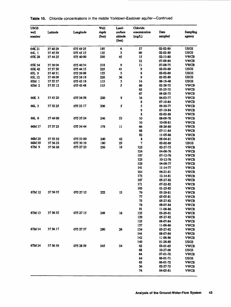
Table 10. Chloride concentrations in the middle Yorktown-Eastover aquifer Continued

USGSwell number

64K2164L 165K28

6SK346SK4265L965L1265M 165M2

66K3

66L3

66L6

66M17

66M2066M3967M 9

67M12

67M13

67M14

67M24

Latitude

374029374559374425

373904373750374931374809375537375512

374320

375225

374900

375723

37 53 32375623375626

375635

375635

375617

375639

Longitude

0754925075 45 150754000

075403407544150753908075381807543180754348

0753656

0753217

0753524

0753444

0753300075 30 190752723

0752715

0752715

0752737

0752859

Well depth (feet)

185135230

218225155220115115

220

206

246

178

240180256

222

249

280

245


65

45

9413

3635

8

5

53

11

422519

13

16

26

24


1769151211989

14666567168598

101066688287

1251241071231291411641731671711837977737881

13512913513713414414214062686464655674

Date sampled

02-02-8902-02-8902-13-8007-09-8407-08-7502-02-8902-02-8902-02-8908-18-4802-28-7503-25-7509-08-7506-03-7707-10-8409-30-7707-10-8402-02-8808-09-7810-08-8108-26-8007-11-8411-05-8608-04-8102-02-8902-27-7504-06-7607-12-7610-12-7604-08-7711-14-7704-21-8112-14-8105-27-8207-22-8201-25-8303-29-8105-05-8105-27-8208-07-8411-06-8603-29-8105-27-8208-07-8411-06-8605-27-8208-07-8411-06-8601-26-8802-01-6510-27-6907-01-7006-01-7106-01-7202-27-7504-05-81

Sflmpling agency

USGSUSGSVWCBVWCBVWCBUSGSUSGSUSGSUSGSVWCBVWCBVWCBVWCBVWCBVWCBVWCBVWCBVWCBVWCBVWCBVWCBVWCBVWCBUSGSVWCBVWCBVWCBVWCBVWCBVWCBVWCBVWCBVWCBVWCBVWCBVWCBVWCBVWCBVWCBVWCBVWCBVWCBVWCBVWCBVWCBVWCBVWCBUSGSVWCBUSGSVWCBUSGSVWCBVWCBVWCB


Table 11 . Chloride concentrations in the lower Yorktown-Eastover aquifer[USGS, U.S. Geological Survey; VWCB, Virginia Water Control Board; latitude and longitude are reported in degrees, arc minutes, arc seconds; mg/L, milligrams per liter]

USGS wdl Latitude number

62F 1 37145763F 16 37 13 07

63G 15 37 17 09

63G23 371653

63G24 371653

63H 4 37 27 05

63H 8 372620

63J 3 373230

64H 5 372922

64J11 373059

64J15 37364264J16 37370564K 5 373828

64K7 373845

Longitude

07600280755835

0755608

0755848

0755848

0755559

0755255

0755410

0764701

0754845

075460807545500754509

0755225

Well depth (feet)

260285

310

280

330

235

295

290

306

313

264262290

176


1231

28

15

15

17

33

22

6

30

394045

8


35875737792

148130130289899

387640630750730630297244246262290

13101212141212

4.8506,2002,2172,1502^502,1001.5981,5101,900

11879

320318306300310

Date sampled

01-01-7808-11-8007-12-84084)4-8609-27-8708-06-84084)4-8602-28-8906-29-7908-19-8007-12-8401-25-8803-01-8906-29-7908-11-8007-12-84084)4-8611-10-8703-01-8909-28-7705-10-7906-26-8408-04-8603-02-8905-02-7911-28-7902-19-8107-21-8209-12-8308-23-8402-19-8506-28-8411-18-8706-01-7707-11-8408-05-8611-12-8707-03-7908-21-8011-10-8708-07-8108-07-8102-28-7509-11-7509-30-7708-20-8006-26-8408-05-8603-02-89

Sampling agency

VWCBVWCBVWCBVWCBVWCBVWCBVWCBUSGSVWCBVWCBVWCBUSGSUSGSVWCBVWCBVWCBVWCBUSGSUSGSVWCBVWCBVWCBVWCBUSGSVWCBVWCBVWCBVWCBVWCBVWCBVWCBVWCBUSGSVWCBVWCBVWCBUSGSVWCBVWCBUSGSVWCBVWCBVWCBUSGSVWCBVWCBVWCBVWCBUSGS


Table 11. Chloride concentrations in the lower Yorktown-Eastover aquifer Continued

USGS well Latitude number

64K 12 37 39 32

65K 7 373805

65K18 373800

65K20 37381065K23 374442

65K25 374442

65K29 374425

65M 3 37 55 12

66K 2 37 43 20

66L 1 375225

66M 5 375239

66M18 375723

66M25 375610

66M26 375610

Longitude

0754527

0754000

0754000

07540000754325

0754325

0754000

075 43 48

0753805

075 32 17

0753529

0753444

0753618

0753618

Well depth (feet)

284

295

283

295290

228

315

195

292

305

246

240

340

230


47

36

40

4313

12

45

5

10

5

17

11

6

6


1212114312373355

515800

91510

226320430330343398130459

1612141716251519241823181917

790755

1,6751,4002,1002,1001,000

810

Date____i_j sampled

08-21-8006-29-8401-26-8809-21-7102-20-7509-20-7102-27-7509-21-7108-13-8002-01-8808-13-8001-27-8808-26-8007-09-8411-11-8702-01-7501-28-8001-20-8204-17-8506-03-8408-06-8601-27-8809-15-7707-10-8402-01-8804-06-5502-26-7603-23-7606-03-7608-31-7612-02-7603-31-7705-31-7709-15-7712-01-7703-06-7808-26-8007-11-8411-05-8610-30-8710-30-8708-29-8810-30-8708-29-88

Sampling agency

VWCBVWCBUSGSUSGSVWCBUSGSVWCBUSGSVWCBUSGSVWCBUSGSVWCBVWCBUSGSVWCBVWCBVWCBVWCBVWCBVWCBUSGSVWCBVWCBUSGSUSGSVWCBVWCBVWCBVWCBVWCBVWCBVWCBVWCBVWCBVWCBVWCBVWCBVWCBUSGSUSGSUSGSUSGSUSGS

chloride concentration. This approach is not intended to provide specific information concerning the physical and chemical nature of the transition zone between freshwater and saltwater. A more detailed examination of the transition zone would require knowledge of the dispersive characteristics of the aquifers. Comparisons between sharp- interface and disperse-interface solutions have

shown that the sharp-interface toe tends to be farther inland than the actual transition zone because the effects of dispersion are neglected (Cooper, 1959; Kohout, 1964; Volker and Rushton, 1982; Hill, 1988). The modeled saltwater-freshwater sharp interface is a first attempt at understanding the saltwater-freshwater-flow dynamics; the sharp inter face provides information concerning the general


GRID CELL COORDINATES ( I, j )

M i+1 /HP

FRESHWA TER

TOE Not to scale

Figure 23. Model representation of the saltwater-freshwater interface tip and toe.

response of the interface to applied stresses. A deri vation of the equations and a complete description of the solution algorithm are provided in Essaid (1990a).

Model Grid and Boundaries

The physical conceptualization of the ground- water-flow system is incorporated into a finite- difference model by dividing the system into a net work of rectangular grid blocks (fig. 24). Each grid block is assigned values that represent the average aquifer characteristics and hydrologic stresses for that area. The spatial discretization for the Eastern Shore ground-water-flow model consists of a vari able three-dimensional grid of 106 rows and 59 col umns. The grid-block dimensions range from a min imum of 0.49 mi to a maximum of 3.29 mi.

The model simulates flow only in the confined aquifers. Each of the three confined aquifers con taining freshwater on the Eastern Shore was repre sented by a separate model layer. The unconfined aquifer was represented as a constant-head boundary overlying the confined-aquifer system. Confining units are not represented by layers but by vertical leakance terms assigned between layers. The physi cal and model conceptualizations of the ground- water-flow system are shown in figure 25. Model grid blocks can contain all freshwater, all saltwater,

or both freshwater and saltwater. When the saltwater-freshwater interface passes through a grid block, the grid block contains both saltwater and freshwater.

The model boundaries are designed to approx imate the actual physical system. The western, east ern, and southern boundaries for the Eastern Shore peninsula are the Chesapeake Bay and the Atlantic Ocean and are represented as no-flow boundaries in the digital flow model. The boundaries are located far enough offshore to include the nearshore saltwater-flow regime. The model simulates the position of the saltwater-freshwater interface bound ary condition. The location of this boundary changes in response to changes in the saltwater-flow and freshwater-flow regimes. The Ghyben-Herzberg approximation was applied to current water-table head values for an initial estimate of the interface position (Heath, 1983). The lower boundary of the model is simulated as a no-flow boundary and approximates the contact between the lower Yorktown-Eastover aquifer and the 150- to 300-ft- thick St. Marys confining unit. This contact also is the lower limit of the freshwater-flow system. The upper boundary of the model is simulated as a constant-head boundary that represents the long-term

Figure 24. Finite-difference grid and boundaries used > in model analysis.


20 MILES

KILOMETERS


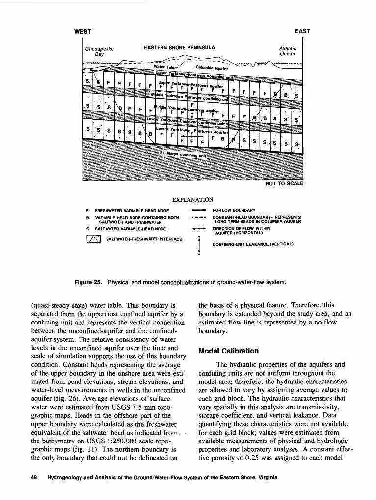
WEST EAST

EASTERN SHORE PENINSULA

NOT TO SCALE

EXPLANATION

F FRESHWATER VARIABLE-HEAD NODE

B VARIABLE-HEAD NODE CONTAINING BOTH SALTWATER AND FRESHWATER

S SALTWATER VARIABLE-HEAD NODE

SALTWATER-FRESHWATER INTERFACE

NO-FLOW BOUNDARY

CONSTANT-HEAD BOUNDARY-- REPRESENTS LONG-TERM HEADS IN COLUMBIA AQUIFER

DIRECTION OF FLOW WITHIN AQUIFER (HORIZONTAL)

CONFINING-UNIT LEAKANCE (VERTICAL)

Figure 25. Physical and model conceptualizations of ground-water-flow system.

(quasi-steady-state) water table. This boundary is separated from the uppermost confined aquifer by a confining unit and represents the vertical connection between the unconfmed-aquifer and the confined- aquifer system. The relative consistency of water levels in the unconfined aquifer over the time and scale of simulation supports the use of this boundary condition. Constant heads representing the average of the upper boundary in the onshore area were esti mated from pond elevations, stream elevations, and water-level measurements in wells in the unconfined aquifer (fig. 26). Average elevations of surface water were estimated from USGS 7.5-min topo graphic maps. Heads in the offshore part of the upper boundary were calculated as the freshwater equivalent of the saltwater head as indicated from the bathymetry on USGS 1:250,000 scale topo graphic maps (fig. 11). The northern boundary is the only boundary that could not be delineated on

the basis of a physical feature. Therefore, this boundary is extended beyond the study area, and an estimated flow line is represented by a no-flow boundary.

Model Calibration

The hydraulic properties of the aquifers and confining units are not uniform throughout the model area; therefore, the hydraulic characteristics are allowed to vary by assigning average values to each grid block. The hydraulic characteristics that vary spatially in this analysis are transrnissivity, storage coefficient, and vertical leakance. Data quantifying these characteristics were not available for each grid block; values were estimated from available measurements of physical and hydrologic properties and laboratory analyses. A constant effec tive porosity of 0.25 was assigned to each model


76° 45' 30' 75° 15'

38 C

45'

30'

37° 15'

EXPLANATION

WATER-LEVEL-CONTOUR-Shows altitude of water level Interval 10 feet. Datum is sea level

-Fishermans Island

20 MILES _I

20 KILOMETERS

Figure 26. Average water levels for the Columbia aquifer.


layer. Model-sensitivity analyses indicated that results were not sensitive to changes in effective porosity.

An iterative process was used to calibrate the ground-water-flow model. Initial estimates of hydraulic properties were used to run a steady-state simulation for prepumping conditions. The initial steady-state results were used as a starting point for a transient simulation of pumping conditions for the period 1940-88. The initial hydraulic properties were adjusted by comparing the simulated water levels to measured water levels. The process was repeated until simulated and measured water levels were in close agreement at all observation wells. The calibrated values used in the model analysis are stored on computer tapes at the Virginia District Office of the USGS in Richmond, Va.

Transmissivity

The transmissivity for each grid block is cal culated by multiplying the average thickness of the aquifer by the average horizontal hydraulic conduc tivity of the aquifer. The average thickness of the aquifer was calculated for each grid block using maps of the tops of aquifers and confining units (figs. 3-9). Initial average horizontal hydraulic con ductivities were estimated from specific-capacity and aquifer-test data. These initial values were adjusted slightly during the transient-model calibration. Actual horizontal hydraulic conductivity data are sparse; therefore, the values were held constant for each layer except in areas where major regional geo logic changes could be discerned. The final horizon tal hydraulic conductivities used in the model analy sis are 51.6, 43.2, and 8.6 ft/d for the upper, middle, and lower Yorktown-Eastover aquifers, respectively (figs. 27-29). The horizontal hydraulic conductivity in the northwestern corner of the model area was reduced to 1.3 ft/d to reflect fine-grained sediments and reduced water-bearing capabilities in the western part of Somerset County, Md. (Werkheiser, 1990). The horizontal hydraulic con ductivity was also reduced 1 order of magnitude near Exmore and near Cape Charles in the middle Yorktown-Eastover aquifer (4.3 ft/d) to reflect the presence of Pleistocene paleochannels in which the original aquifer materials in these areas have been eroded and replaced by sediments with different hydraulic properties. A summary of the range of transmissivities estimated from specific-capacity data

compared with the range of transmissivities used in the final model analysis is given in table 12.

Storage Coefficient

The storage coefficient for each grid block was calculated by multiplying the estimated specific storage of the aquifer by the average saturated thick ness of the aquifer. A constant specific storage of 1 x 10~6/ft is used in the model analysis; the value for specific storage was not calibrated during model development. This value is commonly used in the literature to represent the specific storage of a con fined aquifer and is considered reasonable if all water released from aquifer storage results from the compressibility of water (Lohman, 1979). The range of storage coefficients is listed by aquifer in table 13.

Vertical Leakance

The vertical leakance for each grid block was calculated by dividing the vertical hydraulic conduc tivity of the confining unit by the average thickness of the confining unit (figs. 3-9). A constant vertical hydraulic conductivity of 1.39xlO~5ft/d from labo ratory analysis of core samples (table 4) was used to calculate the initial vertical leakance used in the model calibration. Few core samples are available for the Eastern Shore; therefore, initial estimates were adjusted during transient-model development to estimate areal variations in vertical hydraulic con ductivity. The range of final calibrated values for vertical leakance is listed by confining unit in table 14.

Steady-State-Model Simulation of Prepumping Conditions

Prior to 1940, ground-water withdrawals on the Eastern Shore were minor. Ground-water use consisted of a relatively small number of users with drawing small amounts of water. The ground-water- flow system at this time existed in an approximate state of hydraulic equilibrium (steady state). A steady-state-flow condition is reached when recharge to the system equals discharge from the system. This condition implies that the water levels are constant over time and that the change in storage in the ground-water system is negligible. A steady- state simulation was conducted using prepumping conditions for the Eastern Shore. The steady-state


76 C 45' 30' 75° 15'

38 r

45'

30'

37° 15'

EXPLANATION

AREA WHERE HYDRAULIC CONDUCTIVITY EQUALS 1.3 FEET PER DAY


10I_I

20 MILES

20 KILOMETERS

Figure 27. Hydraulic conductivity of the upper Yorktown-Eastover aquifer based on model calibration.


76 C 45' 30' 75° 15'

38°

45'

30'

37" 15'

EXPLANATION




1U 20 MILES

20 KILOMETERS

Figure 28. Hydraulic conductivity of the middle Yorktown-Eastover aquifer based on model calibration.


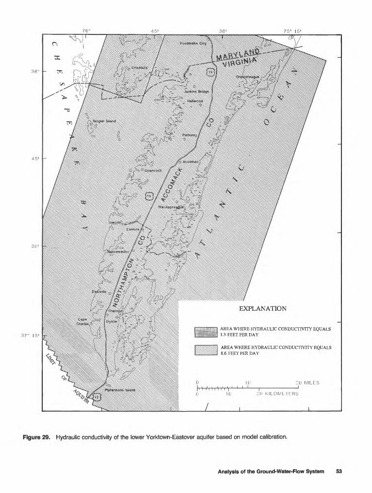
76° 45' 30' 75° 15'

38"

45'

30'

37" 15'AREA WHERE HYDRAULIC CONDUCTIVITY EQUALS 1.3 FEET PER DAY


20 MILES

20 KILOMETERS

Figure 29. Hydraulic conductivity of the lower Yorktown-Eastover aquifer based on model calibration.


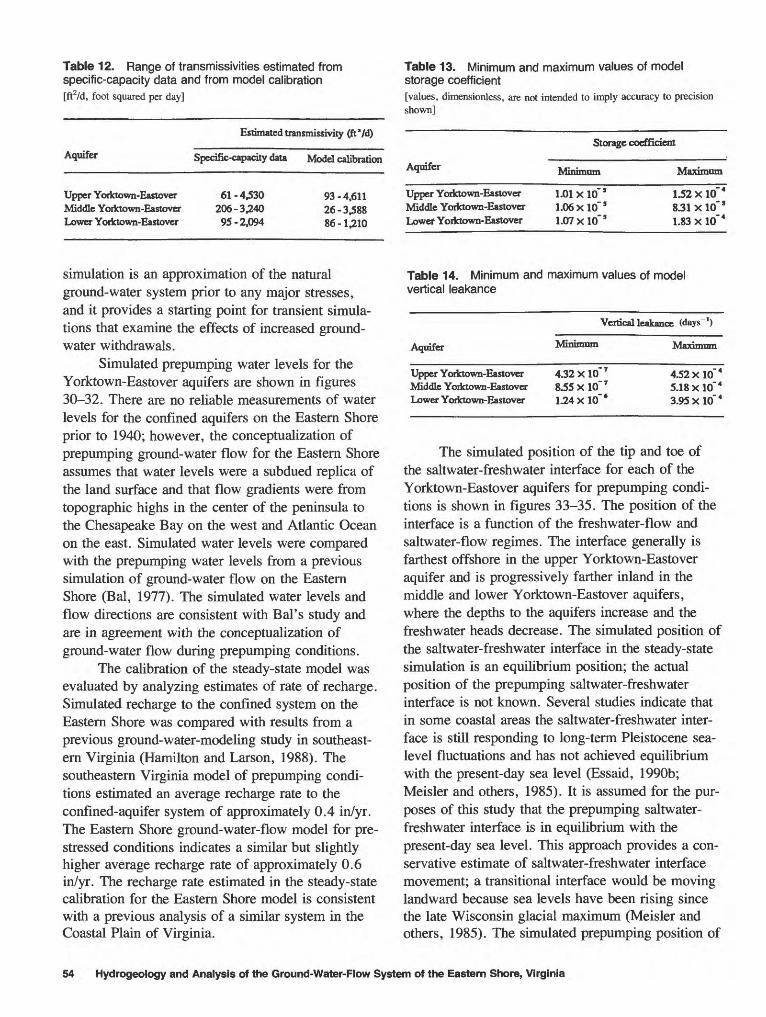
Table 12. Range of transmissivities estimated from specific-capacity data and from model calibration[ft2/d, foot squared per day]

Estimated transmissivity (ft*/d)

Aquifer Specific-capacity data Modd calibration

Upper Yorktown-EastoverMiddle Yorktown-EasloverLower Yorktown-Eastover

61-4.530206-3,24095-2,094

93-4.61126-3.58886-1,210

Table 13. Minimum and maximum values of model storage coefficient[values, dimensionless, are not intended to imply accuracy to precision shown]

Aquifer Minimum

Storage coefficient

Upper Yoiktown-Eastover Middle Yorktown-Eastover Lower Yoiktown-Eastover

1.01 X 10" 5 1.06 X 10" 5 1.07X10' 5

Maximum

L52X10" 4 8J1X10" 1

1.83X10"*

simulation is an approximation of the natural ground-water system prior to any major stresses, and it provides a starting point for transient simula tions that examine the effects of increased ground- water withdrawals.

Simulated prepumping water levels for the Yorktown-Eastover aquifers are shown in figures 30-32. There are no reliable measurements of water levels for the confined aquifers on the Eastern Shore prior to 1940; however, the conceptualization of prepumping ground-water flow for the Eastern Shore assumes that water levels were a subdued replica of the land surface and that flow gradients were from topographic highs in the center of the peninsula to the Chesapeake Bay on the west and Atlantic Ocean on the east. Simulated water levels were compared with the prepumping water levels from a previous simulation of ground-water flow on the Eastern Shore (Bal, 1977). The simulated water levels and flow directions are consistent with Bal's study and are in agreement with the conceptualization of ground-water flow during prepumping conditions.

The calibration of the steady-state model was evaluated by analyzing estimates of rate of recharge. Simulated recharge to the confined system on the Eastern Shore was compared with results from a previous ground-water-modeling study in southeast ern Virginia (Hamilton and Larson, 1988). The southeastern Virginia model of prepumping condi tions estimated an average recharge rate to the confined-aquifer system of approximately 0.4 in/yr. The Eastern Shore ground-water-flow model for pre- stressed conditions indicates a similar but slightly higher average recharge rate of approximately 0.6 in/yr. The recharge rate estimated in the steady-state calibration for the Eastern Shore model is consistent with a previous analysis of a similar system in the Coastal Plain of Virginia.

Table 14. Minimum and maximum values of model vertical leakance

Vertical leakance (days" 1)

Aquifer Maximum

Upper Yorktown-Eastover Middle Yoiktown-Eastover Lower Yorktown-Eastover

4.32 X10~ 7

8.55 X 10" 7 L24XlO~'

4.52X10 ' 5.18 X 10" * 3.95 X 10" *

The simulated position of the tip and toe of the saltwater-freshwater interface for each of the Yorktown-Eastover aquifers for prepumping condi tions is shown in figures 33-35. The position of the interface is a function of the freshwater-flow and saltwater-flow regimes. The interface generally is farthest offshore in the upper Yorktown-Eastover aquifer and is progressively farther inland in the middle and lower Yorktown-Eastover aquifers, where the depths to the aquifers increase and the freshwater heads decrease. The simulated position of the saltwater-freshwater interface in the steady-state simulation is an equilibrium position; the actual position of the prepumping saltwater-freshwater interface is not known. Several studies indicate that in some coastal areas the saltwater-freshwater inter face is still responding to long-term Pleistocene sea- level fluctuations and has not achieved equilibrium with the present-day sea level (Essaid, 1990b; Meisler and others, 1985). It is assumed for the pur poses of this study that the prepumping saltwater- freshwater interface is in equilibrium with the present-day sea level. This approach provides a con servative estimate of saltwater-freshwater interface movement; a transitional interface would be moving landward because sea levels have been rising since the late Wisconsin glacial maximum (Meisler and others, 1985). The simulated prepumping position of


76 C 45' 30' 75° 15'

38 C

45'

30'

37° 15'

EXPLANATION

SIMULATED WATER-LEVEL CONTOUR--Shows altitude of simulated water level. Interval 5 feet Datum is sea level

10MM- ' '

20 MILES

20 KILOMETERS

Figure 30. Simulated water levels in the upper Yorktown-Eastover aquifer for prepumping conditions.


76° 45' 30' 75° 15'

38°

45'

30'

37° 15'

EXPLANATION

SIMULATED WATER-LEVEL CONTOUR-Shows altitude of simulated water level. Interval, in feet, is variable. Datum is sea level

20 MILES

:0 KILOMETERS

Figure 31. Simulated water levels in the middle Yorktown-Eastover aquifer for prepumping conditions.

56 Hydrogeology and Analysis of the Ground-Water-Flew System of the Eastern Shore, Virginia

76 C 45' 30' 75° 15'

38°

45'

30'

37° 15'

EXPLANATION

SIMULATED WATER-LEVEL CONTOUR--Shows altitude of simulated water level. Interval, in feet, is variable. Datum is sea level

10 20 MILES

20 KILOMETERS

Figure 32. Simulated water levels in the lower Yorktown-Eastover aquifer for prepumping conditions.


76° 45' 30' 75° 15'

38 C

45'

30'

37° 15'

SIMULATED STEADY-STATE PREPUMPING INTERFACE TOE

SIMULATED STEADY-STATE PREPUMPING INTERFACE TIP

20 MILES

20 KILOMETERS

Figure 33. Simulated position of the saltwater-freshwater interface for the upper Yorktown-Eastover aquifer for prepumping conditions.


76< 45' 30' 75° 15'

38 C

45'

30'

37° 15'

EXPLANATION



20 MILES I

20 KILOMETERS

Figure 34. Simulated position of the saltwater-freshwater interface for the middle Yorktown-Eastover aquifer for prepumping conditions.


76' 45' 30' 75° 15'

45'

30'

37" 15'

EXPLANATION



10 i i i I

20 MILES

20 KILOMETERS

Figure 35. Simulated position of the saltwater-freshwater interface for the lower Yorktown-Eastover aquifer for prepumping conditions.


the saltwater-freshwater interface is a useful refer ence for examining the relative effects of withdraw als on the ground-water-flow system.

Transient-Model Simulation of Pumping Conditions

A transient-model simulation was conducted to simulate the effects of ground-water withdrawals on the Eastern Shore from 1940 to 1988. The water levels and interface position generated in the prepumping steady-state simulation were used as initial conditions in the transient-model analysis. Aquifer and confining-unit hydraulic characteristics were equivalent to those used when simulating prepumping conditions. The transient simulation shows the effects of historic withdrawals on the ground-water- flow system.

Time Discretization and Ground-Water Withdrawals

Pumpage has varied during the history of ground-water withdrawal on the Eastern Shore (fig. 36). The transient changes in withdrawals are accounted for in the model by dividing historical pumpage into 12 pumping periods. Model-simulated pumping periods are the years 1940^4, 1945-46, 1947-55, 1956-64, 1965-67, 1968-72, 1973-77, 1978-79, 1980-81, 1982-84, 1985-86, and 1987-88. Each pumping period starts on January 1 of its beginning year and ends on December 31 of its final year. Simulated withdrawals were calculated by aquifer for each pumping period from annual withdrawal data (fig. 18) using an average for the time period (fig. 36, table 15). Aquifer-top maps (figs. 3-9) and well-screen depth information were used to assign the withdrawals to the appropriate aquifer. Withdrawals for multiaquifer wells were determined by the percentage of the total screen present in each aquifer.

Results of Simulation

The transient simulation was evaluated by comparing simulated water levels to measured water levels. This comparison was made for a network of 48 observation wells distributed throughout the model area. Water levels for 12 of the observation wells are presented in figures 37-39. The observa tion wells selected are distributed throughout the model area, and water-level changes are representa

tive of the total group of observation wells. Simu lated water levels show reasonable agreement with measured water levels in all of the observation wells for the period of record. Some simulated water lev els are slightly higher than measured water levels and some are slightly lower.

Simulated water levels for 1988 are shown in figures 40-42. Measured water levels are included on these maps to allow comparison between simu lated and measured values. A comparison of simu lated 1988 water levels with prepumping water lev els (figs. 30-32) indicates a decline in water levels around the major pumping centers. The maximum simulated water-level declines in all three aquifers occur near the town of Accomac. Maximum water- level declines are 18, 30, and 53 ft in the upper, middle, and lower Yorktown-Eastover aquifers, respectively. Drawdown cones associated with the major pumping centers indicate a change in ground- water flow from prepumping conditions. Prior to ground-water withdrawals, flow was from the topo graphic highs in the center of the peninsula toward the Chesapeake Bay and Atlantic Ocean (figs. 30-32). By 1988, simulated water-level gradients show that water is diverted toward the major pump ing centers (figs. 40-42). Top-of-aquifer maps can be compared with the simulated water levels to identify areas in which the water levels are approaching the top of the aquifer. Water levels that decline below the top of a confined aquifer cause unconfined conditions in the aquifer and can result in dewatering and associated irreversible changes in the aquifer. Dewatering can contribute to compac tion of aquifer sediment and eventual decreases in aquifer yields. Simulated 1988 water levels are above the tops of the aquifers throughout the model area.

The amount of ground-water flow through the system also is changed as a result of withdrawals. The majority of the water for the increase in with drawals comes from an increase in the amount of water recharging the confined-aquifer system from the unconfined aquifer and a decrease in the amount of discharge to the unconfined aquifer. In areas where pumpage causes water levels to decline in the confined aquifers, the head difference between the unconfined-aquifer and the confined-aquifer system increases. The increased head difference causes an increase in vertical leakage through the confining unit, and some freshwater that was previously discharging from the unconfined aquifer to


AVERAGE WITHDRAWAL SIMULATED FOR PUMPING PERIOD

DC LU Q.

COZo_l _l

oz o

DC Qn:

ESTIMATED ANNUAL WITHDRAWAL

1940 1945 1950 1955 1960 1965 1970 1975 1980 1985 1990

Figure 36. Estimated annual withdrawal and average withdrawal for simulated pumping periods.

surface-water bodies is diverted and flows into the confined-aquifer system. Any increase in withdraw als from the freshwater aquifers on the Eastern Shore results in a reduction in offshore freshwater discharge. A reduction in freshwater discharge affects the long-term position of the saltwater- freshwater interface in the aquifers and could cause increased salinity in sensitive estuarine environ ments. The steady-state prepumping simulation indi cates that 11.07 Mgal/d recharges and discharges the confined ground-water-flow system (table 16). When 1988 withdrawals are simulated, the recharge to the confined aquifers increases to 13.11 Mgal/d, and natural discharge decreases to 8.64 Mgal/d.

The transient simulation of conditions for the period 1940-88 shows no movement of the

saltwater-freshwater interface, although significant changes in the flow system occur. The simulated position of the saltwater-freshwater interface for 1988 conditions is identical to the simulated inter face position for prepumping conditions (figs. 33-35). This result indicates that interface response is slow and takes place over long periods of time. Similar findings have been recorded in other saltwater-intrusion studies (Bond and Bredehoeft, 1987; Essaid, 1990b; Meisler and others, 1985). The investigation by Bond and Bredehoeft (1987) using a two-dimensional solute-transport model showed the main pathway for saltwater intrusion over short timeframes was downward vertical leak age of saltwater from surface-water bodies into the shallow aquifers. Simulated water-level gradients for


|1

°3'Ss,2

i_ ay> 2 j oof ^

*>* "ON-° 6

| 2

O) «JC B'5. «E SQ. |

0 >^s §o 8,W B« |5 ^ 2 -a o o

|1

in .B

_« S

§ 1

j8

M

1

,?

a is

ZH OOo\

o ci

oo

ON oo

oo00 S\

en'"-

f?

VO ^P

5?-S

^^

^22

tnW">

oK^^

* "is

-1

1

§Soo"

1

is

Ji^

o\oo"

1

ooo

o

o

1

6

>

1

Upper Yoiktow

S

J2c<M

i

i

1enen

00ooo\~

s

^H00

i

i

{«

1Middle Yoikto

i

§p"

So

00

§

1rt

"1

1

i

^*

g

?

i

si1Lower Yotktov

i00en«o

1

1

oo

s5VO00

3~

1

s

!Q8

o

6

I


WE

LL

67M

14

I i <D 2. f

o> <D

O

O i 3

i (0 o S I! 3 5'

10 0

-10

20 -30 40

i M

I

I I

I l-14-L

-LLi.LLLLLL

1 '

' '

' '

' '

'

uj

WE

LL

64H

7>

WE

LL

63F

17

I I

I M

I

I I

I 1

I I

I I

I I

I I

I I

I I

| |

I

<

6HI C/

3 3

I

0

HI

CO

-3DC O

-6

HI 5 <

18H

-LL

J 15

HI

U_ ^r

12

-I

9H

I

UJ

6_

l

DC

3 H

I I

WE

LL

66K

312

I I

I I

I I

H-L

J.J

_L

I I

I

\

0 20

KIL

OM

ET

ER

S

EX

PL

AN

AT

ION

M

EA

SU

RE

D W

AT

ER

LE

VE

L

S

IMU

LA

TE

D W

ATE

R L

EV

EL

67

M1

4

W

EL

L A

ND

ID

EN

TIF

IER

1940

19

50

1960

19

70

1980

19

90

Figu

re 3

7.

Sim

ulat

ed a

nd m

easu

red

wat

er le

vels

at s

elec

ted

obse

rvat

ion

wel

ls in

the

uppe

r Y

orkt

own-

Eas

tove

r aq

uife

r.

__Z

XLU

LU LU> >LU LU I IDC DCLU LU

i iQ QLU LUtt t3 <(0 d< iLU 52 53

QC LU

LU O

_J

LU

2cr> cr>

I

CO Litc

I I

co -

co co

LU I

(: i\ i

iii- i- i - ii- ir /_ i

- i- i- i- i- i - i - i

_~_-

-

-

_---I---

O)

co :

LU :

- '' -L±- ' -^^-'^- i ^- i s:VV- F2

\: />

/-r: i- 1-i :i _i_i -i-i -iH-r- -f1TI4fTLii

i i

i i-~-~~

:^

, _

^

~"

-- ~~~_-~

_

-

i i

OCOco

LU

CM_Jco co

LU -

T T T

13A3T V3S MO138 dO 3AC9V 133d Nl '13A31 U31VM

CO

i-Q O

CD

I 1

|

CO o

E co

O)


WE

LL

66

M1

8

£. < ss.CO* o (D o

3 a i V) o

LJJ

>

LJJ

LJJ

C/3

O LJJ

CO CC O LJJ O CO LJJ

LJJ

LJJ

>

LJJ

-J CC

LU s

6 3 0 -3 -6 8 7 6 5 4 3

12

8 4 0 -4 -8

^v

WE

LL

63H

4I

I I

I M

I

M_[_

M

I I

I I

I I

I I

I M

I

M

I I

I |

I M

I

I I

I I

I I

I I

I I

I I

I i r

WE

LL

65K

23

I I

I I

20

KIL

OM

ET

ER

S

WE

LL

63G

24

4 0 -4 -8

-12

1111

111

Hin

j.LLLL

1' I'' '' '''''

I'' '''''' '

I '''' '''' '

EX

PL

AN

AT

ION

ME

AS

UR

ED

WA

TE

R L

EV

EL

S

IMU

LA

TE

D W

AT

ER

LE

VE

L

66

M1

8

W

EL

L A

ND

ID

EN

TIF

IER

19

40

1950

19

60

1970

19

80

19

90

Figu

re 3

9.

Sim

ulat

ed a

nd m

easu

red

wat

er le

vels

at

sele

cted

obs

erva

tion

wel

ls in

the

low

er Y

orkt

own-

Eas

tove

r aq

uife

r.

76° 45' 30' 75° 15'

38°

45'

30'

37° 15'

EXPLANATION

SIMULATED WATER-LEVEL CONTOUR-Shows altitude of simulated water level. Hachures indicate depression. Interval, in feet, is variable. Datum is sea level

WELL--Number is measured altitude of water level, in feet above sea level

:o MILE:

?0 KILOMETERS

Figure 40. Simulated and measured water levels in the upper Yorktown-Eastover aquifer, 1988.


76 C 45' 30' 75° 15'

38 C

45'

30'

37° 15'

EXPLANATION

SIMULATED WATER-LEVEL CONTOUR-Shows altitude of simulated water level. Interval, in feet, is variable. Datum is sea level

WELL Number is measured altitude of water level, in feet above or below sea level

20 MILES

20 KILOMETERS

Figure 41. Simulated and measured water levels in the middle Yorktown-Eastover aquifer, 1988.


76° 45

45' -

EXPLANATION

SIMULATED WATER-LEVEL CONTOUR--Show altitude of simulated water level. Interval, in feet, is variable. Datum is sea level

WELL Number is measured altitude of water level, in feet above or below sea level

20 KILOMETERS

37° 15' -

Figure 42. Simulated and measured water levels in the lower Yorktown-Eastover aquifer, 1988.


Tabl

e 16

. S

imul

ated

gro

und-

wat

er b

udge

ts f

or th

e co

nfin

ed f

resh

wat

er-fl

ow s

yste

m[M

odel

ed v

alue

s, i

n m

illio

n ga

llons

per

day

, ar

e no

t in

tend

ed t

o im

ply

accu

racy

to

prec

isio

n sh

own;

the

sm

all

erro

r be

twee

n so

urce

s an

d di

scha

rges

is

due

to n

umer

ical

tru

ncat

ion

in d

igita

l si

mul

atio

n; ,

budg

et c

ompo

nent

not

app

licab

le t

o th

e si

mul

atio

n]

>logy and

Analysis of

tl he

Ground-Wa 5 Tj f a (D s O 9 c3 3 5*

Bud

get

com

pone

nt

Prep

umpi

ng

Sour

ce

Rec

harg

e to

11

.07

conf

ined

sys

tem

th

roug

h up

perm

ost

conf

inin

g un

it

Wat

er re

leas

ed fr

om

.00

aqui

fer s

tora

ge

Late

ral b

ound

ary

cons

tant

-hea

d no

des

Tota

l 11

.07

Dis

char

ge

Nat

ural

dis

char

ge

1 1 .0

8 fr

om c

onfin

ed s

yste

m

thro

ugh

uppe

rmos

t co

nfin

ing

unit

Gro

und-

wat

er

.00

with

draw

als f

rom

w

ells

Wat

er ta

ken

into

.0

0 aq

uife

r sto

rage

Sim

ulat

ion

1988

So

uthe

rn

Sout

hern

N

orth

east

ern

Nor

thea

ster

n Pe

rmitt

ed

cond

ition

s N

orth

ampt

on

Nor

tham

pton

A

ccom

ack

Acc

omac

k w

ithdr

awal

si

mul

atio

n 1

sim

ulat

ion

2 si

mul

atio

n 1

sim

ulat

ion

2

13.1

1 14

.93

14.6

3 14

.18

12.8

4 17

.44

.64

.87

.96

1.09

1.

09

1.92

1.47

13.7

5 15

.80

15.5

9 15

.27

15.4

0 19

.36

8.64

7.

52

7.29

8.

11

8.27

5.

65

5.05

8.

24

8.26

7.

10

7.10

13

.70

.00

.00

.00

.00

.00

.00

"Lat

eral

boun

dary

co

nsta

nt-h

ead

node

s.0

0

Tota

l11

.08

13.6

915

.76

15.5

515

.21

15.3

719

.35

1988 conditions on the Eastern Shore show that there is no potential for downward vertical leakage of saltwater through the upper Yorktown-Eastover confining unit above the freshwater part of the upper Yorktown-Eastover aquifer.

The slow movement of the saltwater- freshwater interface was investigated using a tran sient simulation that continued 1988 withdrawals for 1,000 years. The model-simulated interface did not reach an equilibrium position for 1988 withdrawals by the end of the 1,000-year simulation period. The simulated position of the saltwater-freshwater inter face toe for the 1,000-year run is shown along with the 1988 interface in figures 43^5. The position of the interface toe is shown because it is the most landward extension of the saltwater-freshwater inter face. The locations of greatest interface movement in each aquifer correspond to the areas of greatest pumpage. Although the transient simulation from 1940 to 1988 shows no movement of the interface toe from the prepumping steady-state simulation, continuing 1988 withdrawals for 1,000 years causes landward movement of the interface toe along most of the coast in all three aquifers. The interface toe at the southern end of Northampton County in the upper Yorktown-Eastover aquifer (fig. 43) moved approximately 1 mi landward on the bay side of the peninsula and 0.5 mi landward on the ocean side of the peninsula. The interface toe also moved land ward approximately 1 mi in the upper Yorktown- Eastover aquifer near the town of Chincoteague. Maximum landward movement of the interface toe is approximately 1.5 mi in the middle Yorktown- Eastover aquifer (fig. 44), also near the town of Chincoteague. The interface toe moves landward a maximum of approximately 1 mi in the lower Yorktown-Eastover aquifer (fig. 45) southwest of Chincoteague. The results of this simulation support previous findings that movement of the saltwater- freshwater interface is slow and takes place over long periods of time. It is important to remember, however, that a sharp-interface model provides no information on the rate of movement of dilute salt water in the transition zone.

Application of Ground-Water-Flow Model

The prepumping, steady-state-model analysis and the historical transient-model analysis indicate that the model conceptualization is a reasonable rep resentation of the ground-water-flow system of the

Eastern Shore. Three scenarios of hypothetical increases in ground-water withdrawals were devel oped in cooperation with Accomack County, Northampton County, and the VWCB. The results of the simulations of the scenarios are examined to increase our understanding of the response of the ground-water-flow system to additional stress. The simulations are not intended to predict exact ground- water conditions in the future; however, the results provide information that could be useful in evaluat ing the ground-water resource and its ability to meet future water needs.

Southern Northampton County Scenario

The southern part of Northampton County is experiencing rapid growth. Protection of the ground- water resource in this area is of concern because most of the expected development is in coastal areas that could be susceptible to saltwater intrusion. In this scenario, withdrawals are increased in the southern part of Northampton County, and currently permitted users as well as potential projected users are included. The scenario consists of two separate model simulations that illustrate the effects of increased withdrawals with two different well distri butions. In simulation 1, withdrawals are increased to permitted levels at existing well locations, and additional withdrawal wells are placed in the vicin ity of expected growth areas (fig. 46). In simulation 2, withdrawals are increased by the same amount but are distributed evenly throughout hypothetical well fields in the center of the peninsula.

Simulation 1

Results from the transient simulation of 1988 conditions were used as initial conditions for a 50-year transient simulation to examine the effects of increased withdrawals in the southern part of Northampton County. A summary of locations and rates of hypothetical withdrawals and aquifers pene trated for the southern part of Northampton County in simulation 1 is presented in table 17. Total with drawal for the area is 3.761 Mgal/d, which repre sents an increase of 3.213 Mgal/d over 1988 with drawal. Withdrawals from existing wells in the southern part of the peninsula are increased to their permitted levels. Additional withdrawal wells were located by the VWCB according to preliminary or expected permit applications (fig. 46). Approxi mately 57, 29, and 14 percent of the additional


76 C 45' 30' 75° 15'

38 C

45'

30'

37° 15'

SIMULATED 1988 INTERFACE TOE

SIMULATED INTERFACE TOE AFTERSIMULATION OF 1988 \VTTIIDRAWALS

10 20 KILOMETERS

Figure 43. Simulated position of the saltwater-freshwater interface toe for a 1,000-year transient run using 1988 with drawals in the upper Yorktown-Eastover aquifer.


76° 45' 30' 75 C 15'

38 C

45'

30'

37° 15'

EXPLANATION


SIMULATED INTERFACE TOE AFTER 1,000-YEAR SIMULATION OF 1988 WITHDRAWALS

10 i i I

20 MILES

20 KILOMETERS

Figure 44. Simulated position of the saltwater-freshwater interface toe for a 1,000-year transient run using 1988 with drawals in the middle Yorktown-Eastover aquifer.


76° 45' 30' 75° 15'

38°

45'

30'

37° 15'

EXPLANATIONSIMULATED 1988 INTERFACE TOE

SIMULATED INTERFACE TOE AFTER 1,000-YEAR SIMULATION OF 1988 WITHDRAWALS

0 10 20 MILES

20 KILOMETERS

Figure 45. Simulated position of the saltwater-freshwater interface toe for a 1,000-year transient run using 1988 with drawals in the lower Yorktown-Eastover aquifer.


10 M

ILE

S

10

KIL

OM

ET

ER

S

Figu

re 4

6.

Loca

tion

of h

ypot

hetic

al w

ithdr

awal

s fo

r th

e so

uthe

rn N

orth

ampt

on C

ount

y sc

enar

io,

sim

ulat

ion

1.

Table 17. Withdrawals for southern Northampton County scenario, simulation 1[Mgal/d, million gallons per day; latitude and longitude are reported in degrees, arc minutes, arc seconds]

Map number 1

123456789

101112

13141516

Latitude

37 13 3637 13 1437 13 5337 13 5437143537145637145537152037 15 2837172037 17 20371746

37 17 15371711371540371605

Longitude

076001907600210755923075 59 08076003407600520760008076003107559560760051075 58 100755728

075 55 12075552407601210760019

Withdrawal (Mgal/d)

0.047.047.093.093.200.200.200.200.200.004.190

1.600

.150

.152

.125

.260

Aquifer penetrated

Upper Yorktown-EastoverUpper Yorktown-EastoverUpper Yorktown-EastoverUpper Yorktown-EastoverUpper Yorktown-EastoverUpper Yorktown-EastoverUpper Yorktown-EastoverUpper Yorktown-EastoverUpper Yorktown-EastoverUpper Yorktown-EastoverUpper Yorktown-EastoverUpper, middle, andlower Yorktown-Eastover

Middle Yorktown-EastoverMiddle Yorktown-EastoverUpper and middle Yorktown-EastoverUpper and middle Yorktown-Eastover

'Locations shown on figure 46.

pumpage comes from the upper, middle, and lower Yorktown-Eastover aquifers, respectively. Pumpage for the rest of the model area is held constant at the average pumping rate for the final pumping period (pumping period 12) in the historic transient simula tion. Total withdrawals for the entire model area for simulation 1 are greatest in the upper Yorktown- Eastover aquifer and least in the lower Yorktown- Eastover aquifer (table 18).

The hypothetical increased pumpage in the southern part of Northampton County results in water-level declines of greater than 15 ft in each of the confined freshwater aquifers (figs. 47^9). The maximum water-level decline for the upper Yorktown-Eastover aquifer is 16.2 ft near the town of Cape Charles. Maximum water-level declines of 38.8 and 48.7 ft occur east of the town of Cheriton for the middle and lower Yorktown-Eastover aqui fers, respectively (table 19). The predicted declines are in addition to declines caused by ground-water withdrawals in 1988. Simulated water levels throughout the model area remain above the tops of the aquifers, indicating that dewatering would not occur at this rate and distribution of withdrawal.

The majority of the water for the increased ground-water withdrawal is provided by an increase in the amount of recharge entering the confined sys tem and a decrease in the amount of discharge leav ing the confined system (table 16). The simulated

water budget presented in table 16 is for the con fined freshwater-flow system; the withdrawal amounts are slightly less than the total ground-water withdrawals for the simulations (table 18) because a small part of the withdrawals are from the saltwater- flow system. The increase in freshwater withdrawal of 3.19 Mgal/d in the southern part of Northampton County causes a 1.82 Mgal/d increase in the amount of recharge to the confined aquifer system over 1988 conditions. The amount of natural discharge from the confined aquifers is reduced by 1.12 Mgal/d from 1988 conditions.

The 50-year simulation of increased pumpage in southern Northampton County results in slight landward movement of the simulated saltwater- freshwater interface on the Chesapeake Bay side of the peninsula off Cape Charles (figs. 47^9). The interface toe in the upper Yorktown-Eastover aquifer moves inland from the 1988 interface toe position along approximately 12 mi of the western coastline in southern Northampton County (fig. 47); maxi mum landward movement is approximately 1 mi. The simulated position of the interface toe in the middle Yorktown-Eastover aquifer does not change in response to the hypothetical increase in withdraw als. Slight landward movement of the saltwater- freshwater interface toe occurs in the lower Yorktown-Eastover aquifer (fig. 49). The simulated 1988 interface toe position is onshore at this loca-


Table 18. Withdrawal by aquifer for model scenarios[Values in millions of gallons per day]

Aquifer

Upper Yorktown-Eastover Middle Yorktown-Eastover Lower Yorktown-Eastover

Pumping period 12 (1987-88)

1.888 2.103 1.070

Scenario

Southern Northampton simulation 1

3.801 2.915 1.558

Southern Northampton simulation 2

2.951 3.088 2.235

Northeastern Accomack simulations 1&2

2J31 3.431 1.201

Permitted withdrawal

4.446 6.959 2.419

Total 5.061 8.274 8.274 7.163 13.824

Table 19. Maximum water-level decline from 1988 flow conditions for model scenarios

Aquifer Decline (feet)

Grid row

Grid column

Approximate area! location



Southern Northampton County simulation 1 16.2 85 24 38.8 80 29 48.7 80 26

Southern Northampton County simulation 2 8.0 68 26

22.0 76 26 22.4 76 26

Northeastern Accomack County simulation 1

Town of Cape Charles East of Cheriton Town of Cheriton

Town of Nassawadox To\vnofEastviHe Town of Eastville

Upper Yorktown-EastoverMiddle Yorktown-EastoverLower Yorktown-Eastover

17.229.726.4

191919

343434

TownofHallwoodTown of Hall woodTownofHallwood

Northeastern Accomack Countv simulation 2Upper Yorktown-EastoverMiddle Yorktown-EastoverLower Yorktown-Eastover

Upper Yorktown-EastoverMiddle Yorktown-EastoverLower Yorktown-Eastover

15.827.924.6

29.195.368.0

191919

Permitted withdrawal565634

343434

282832

TownofHallwoodTownofHallwoodTown of Hall wood

Town of ExmoreTown of ExmoreTown of Accomac

tion on the southern tip of the peninsula. The hypo thetical increase in withdrawals causes the western boundary of the 1988 interface position to move approximately 0.5 mi in the lower Yorktown- Eastover aquifer.

Although saltwater intrusion due to horizontal movement of the saltwater-freshwater interface takes place over long periods of time, saltwater intrusion due to induced downward vertical leakage can occur rapidly as a result of large changes in head gradient. Simulated water levels show offshore water-level declines that cause a reversal of ground-water flow from 1988 conditions (fig. 47). Simulated water- level declines in the upper Yorktown-Eastover aqui fer show that the increased withdrawals on the coast

cause drawdowns of greater than 5 ft to extend off shore. The area of reversed flow indicates a poten tial for downward vertical leakage of saltwater from the Chesapeake Bay and nearshore estuaries into the freshwater part of the upper Yorktown-Eastover aquifer. The amount of saltwater that is introduced into the freshwater system vertically through the confining unit is probably relatively small; however, salt concentrations could be high and could signifi cantly affect the quality of the water withdrawn. This area is further complicated because of the present-day channel in the Chesapeake Bay (figs. 3 and 11). The upper Yorktown-Eastover confining unit probably has been eroded, and rates of saltwa ter intrusion could be increased because of a direct


76 C 45' 30' 75° 15'

38"

45'

30'

37° 15'

EXPLANATION

AREA OF REVERSED SALTWATER FLOW

5 LINE OF EQUAL MODELED WATER-LEVEL DECLINE FROM SIMULATED 1988 WATER LEVELS-Literal, in feet, is variable


SIMULATED INTERFACE TOE RESULTING FROM SOUTHERN NORTHAMPTON, SIMULATION 1 WITHDRAWALS

10' ' '

20 MILES

10 20 KILOMETERS

Figure 47. Water-level decline from simulated 1988 water levels, simulated position of the saltwater-freshwater interface toe, and area of reversed saltwater flow in the upper Yorktown-Eastover aquifer, southern Northampton County scenario, simulation 1.


76° 45' 30' 75° 15'

38 C

45'

30'

37° 15'

EXPLANATION

LINE OF EQUAL MODELED WATER-LEVEL DECLINE FROM SIMULATED 1988 WATER LEVELS--Interval, in feet, is variable


10MM- ' '

20 MILES

I 10 20 KILOMETERS

Figure 48. Water-level decline from simulated 1988 water levels and simulated position of the saltwater-freshwater inter face toe in the middle Yorktown-Eastover aquifer, southern Northampton County scenario, simulation 1.


76' 45' 30' 75° 15'

38"

45'

30'

37° 15'

EXPLANATION

LINE OF EQUAL MODELED WATER-LEVEL DECLINE FROM SIMULATED 1988 WATER LEVELS-Interval 5 feet


SIMULATED INTERFACE TOE RESULTING FROM SOUTHERN NORTHAMPTON, SIMULATION 1 WITHDRAWALS

10 I I

20 MILES

Figure 49. Water-level decline from simulated 1988 water levels and simulated position of the saltwater-freshwater inter face toe in the lower Yorktown-Eastover aquifer, southern Northampton County scenario, simulation 1.


connection between the upper Yorktown-Eastover aquifer and the saltwater in the Chesapeake Bay. The model results indicate that the hypothetical increase in pumpage in southern Northampton County at current well locations could create water- quality problems. Heavy pumpage along the coast in the upper Yorktown-Eastover aquifer could cause water levels to decline offshore and induce leakage of saltwater from the Chesapeake Bay into the fresh water part of the aquifer. The amount of water- quality degradation that could result from this proc ess cannot be quantified by this study. Model results indicate that this is a potential concern and needs to be considered in future studies.

Simulation 2

In the second simulation, withdrawals are increased in southern Northampton County by the same amount as simulation 1; however, the with drawals are removed from the coast and redistrib uted throughout Northampton County to hypothetical well fields in the center of the peninsula. The total withdrawal for the area is divided equally among 10 hypothetical well fields and is distributed equally among all three confined aquifers (table 20). Pump- age for the rest of the model area is held constant at the average pumping rate for the final pumping period in the historic transient simulation (1987-88). As in the previous simulation, the results of the transient simulation of 1988 conditions are used as initial conditions, and the simulation is continued for a period of 50 years. Withdrawals by aquifer are presented in table 18 for all of the model scenarios.

Modeled water-level declines from simulated 1988 water levels are shown in figures 50-52. Declines are centered in the middle of the peninsula, and the maximum water-level declines are 8.0, 22.0, and 22A ft for the upper, middle, and lower Yorktown-Eastover aquifers, respectively (table 19). Since pumpage is no longer concentrated in the Cape Charles area, water-level declines are smaller in each aquifer for simulation 2 than they are in simulation 1. Water-level declines are greatest in the lower Yorktown-Eastover aquifer because transmissivities are smaller there than in the middle or upper Yorktown-Eastover aquifers. The placement of the wells in the center of the peninsula causes the water-level contours to follow the shape of the peninsula, and less drawdown occurs in offshore areas. As in simulation 1, the simulated water levels

Table 20. Location of southern Northampton scenario withdrawals, simulation 2[Mgal/d, million gallons per day]

Grid location Withdrawal ________ (Mgal/d)

Aquifer

Row Column

64666870727476788082

26262626262626262626

0376376376376376376376376376376

Upper, middle, and lower Yorktown-EastoverUpper, middle, and lower Yorktown-EastoverUpper, middle, and lower Yorktown-EastoverUpper, middle, and lower Yorktown-EastoverUpper, middle, and lower Yorktown-EastoverUpper, middle, and lower Yorktown-EastoverUpper, middle, and lower Yorktown-EastoverUpper, middle, and lower Yorktown-EastoverUpper, middle, and lower Yorktown-EastoverUpper, middle, and lower Yorktown-Eastover

throughout the model area remain above the top of the aquifers.

The simulated ground-water budgets for the freshwater-flow system indicate recharge to the con fined system increases by 1.52 Mgal/d over 1988 conditions, whereas natural discharge from the con fined aquifers decreases by 1.35 Mgal/d from the simulated 1988 discharge rate (table 16). The change in flow through the system is a result of the 3.21 Mgal/d increase in freshwater withdrawals over 1988 rates. Although the total ground-water with drawal for simulation 1 is identical to simulation 2, the freshwater withdrawal is slightly less. The with drawal locations in simulation 1 are near the coast and result in more withdrawal from the saltwater- flow system. A comparison of recharge and dis charge for the two southern Northampton simula tions shows that the same withdrawal amount and a different areal distribution can produce a change in the flux through the system. Slightly less water (0.30 Mgal/d) enters the confined system in simula tion 2, and slightly less water (0.23 Mgal/d) is discharged naturally from the confined system. The decrease in flow through the system in simulation 2 is balanced by a small increase in the amount of water that is released from aquifer storage (table 16).

Slight landward movement of the simulated saltwater-freshwater interface from the 1988 position occurs during the 50-year transient simulation in the upper Yorktown-Eastover aquifer (fig. 50). The interface position for the middle and lower Yorktown-Eastover aquifers does not change from


38° -

45' -

EXPLANATION

LLNE OF EQUAL MODELED WATER-LEVEL DECLINE FROM SLMULATED 1988 WATER LEVELS-Interval, in feet, is variable

SLMULATED 1988 INTERFACE TOE

SLMULATED INTERFACE TOE RESULTING FROM SOUTHERN NORTHAMPTON, SIMULATION 2 WITHDRAWALS

20 KILOMETERS

37" 15' -

Figure 50. Water-level decline from simulated 1988 water levels and simulated position of the saltwater-freshwater interface toe in the upper Yorktown-Eastover aquifer, southern Northampton County scenario, simulation 2.


76° 45' 30' 75° 15'

38"

45'

30'

37" 15' LINE OF EQUAL MODELED WATER-LEVEL DECLINE FROM SIMULATED 1988 WATER LEVELS-Interval, in feet, is variable

SIMULATED 198 8 INTERFACE TOE

1C) i I

20 MILES

Figure 51. Water-level decline from simulated 1988 water levels and simulated position of the saltwater-freshwater interface toe in the middle Yorktown-Eastover aquifer, southern Northampton County scenario, simulation 2.


76 C 45' 30' 75° 15'

38 C

45'

30'

37° 15' LINE OF EQUAL MODELED WATER-LEVEL DECLINE FROM SIMULATED 1988 WATER LEVELS-Interval, in feet, is variable


10 j_I

20 MILES i

20 KILOMETERS

I________________I

Figure 52. Water-level decline from simulated 1988 water levels and simulated position of the saltwater-freshwater interface toe in the lower Yorktown-Eastover aquifer, southern Northampton County scenario, simulation 2.


the 1988 position. The simulated interface toe moves landward a maximum of approximately 0.5 mi in the upper Yorktown-Eastover aquifer. Although the position of the interface does not move as much as it did in simulation 1, this model result illustrates the sensitivity of the fresh-ground-water system in southern Northampton County. The addi tional withdrawal of 3.21 Mgal/d results in some movement of the saltwater-freshwater interface in the uppermost confined aquifer, even with well fields placed as far away from the interface as possi ble. The peninsula in this area is narrow (4-5 mi wide), which limits its ability to sustain large ground-water withdrawals.

Simulated water levels show that saltwater intrusion into the uppermost confined aquifer through downward vertical leakage does not occur when withdrawals are distributed equally to all three aquifers and placed in the center of the peninsula. Freshwater is flowing from the upper Yorktown- Eastover aquifer; water-level declines offshore are not large enough to reverse the hydraulic gradient and induce saltwater leakage through the confining unit.

Northeastern Accomack County Scenario

Chincoteague Island is a popular tourist loca tion in northeastern Accomack County that requires a large supply of freshwater in the summer months. This area is on the easternmost boundary of the Eastern Shore's freshwater-flow system and has a high potential for water-quality degradation by salt water intrusion. The northeastern part of Accomack County has several major ground-water users, and in this scenario, the response of the ground-water-flow system to increased withdrawals is examined.

Two simulations are included in this scenario in order to evaluate model-boundary effects. The scenario consists of large increases in withdrawals over calibrated 1988 conditions in the northeastern corner of the model grid. At this level of with drawal, the effects of the increased stress extend to the northern and eastern boundary of the model; therefore, the results of the simulation are affected by the model-boundary conditions. The boundary effects were quantified by simulating two different types of boundary conditions. In simulation 1, a no-flow boundary (no water available across the boundary) is used to represent the most severe case, namely, maximum water-level decline. In simulation

2, a constant-head boundary (an unlimited supply of water across the boundary) is used to represent a less severe case, or minimum water-level decline. The response of the actual ground-water system would most likely fall somewhere between the two cases.

The initial conditions for both 50-year tran sient simulations of increased withdrawals in north eastern Accomack County are provided by the results of the transient simulation of 1988 condi tions. Withdrawal locations are near the shore of the peninsula (fig. 53); the total hypothetical withdrawal for the area is 3.5 Mgal/d (table 21), an increase of 2.05 Mgal/d over 1988 withdrawals. Approximately 31, 63, and 6 percent of the total withdrawals come from the upper, middle, and lower Yorktown- Eastover aquifers, respectively (table 18). Pumpage for the rest of the model area was held constant at the average pumping rate for the final pumping period in the historic transient simulation (1987-88). The withdrawals for these scenarios are concentrated in the upper two aquifers because the area is too far east to obtain good-quality water from the lower Yorktown-Eastover aquifer. Many of the withdraw als in this area come from the unconfined aquifer, which is not included in this model; therefore, the pumpage for simulations 1 and 2 is lower than the total projected increase for the northeastern part of Accomack County.

Simulation 1: No-Flow Boundary

The results of simulation 1 show that modeled water levels decline from simulated 1988 water lev els throughout much of the northern model area (figs. 54-56). The maximum water-level declines are 17.2, 29.7, and 26.4 ft for the upper, middle, and lower Yorktown-Eastover aquifers, respectively (table 19). The location of the maximum water-level decline is near the town of Hallwood for all three aquifers. Simulated water levels are above the tops of the aquifers, indicating that the dewatering of the confined aquifers is not a concern for this simulation.

The simulated ground-water budget for the freshwater-flow system is presented in table 16. The increase in freshwater withdrawals of 2.05 Mgal/d over 1988 amounts results in a 1.07 Mgal/d increase in flow into the confined system and a 0.53 Mgal/d decrease in natural flow out of the confined system.


10

MIL

ES

10

KIL

OM

ET

ER

S-

Figu

re 5

3.

Loca

tion

of h

ypot

hetic

al w

ithdr

awal

s in

the

nor

thea

ster

n A

ccom

ack

Cou

nty

scen

ario

s.

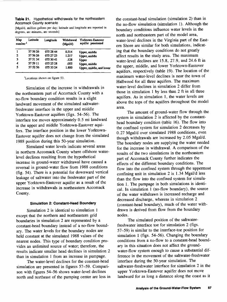
Table 21 . Hypothetical withdrawals for the northeastern Accomack County scenario[Mgal/d, million gallons per day; latitude and longitude are reported in degrees, arc minutes, arc seconds]

Map Latitudenumber 1

1 3756262 3756263 3751344 3759115 375256

Longitude

07528440752723075304107525280753324

Withdrawal(Mgal/d)

0.3141.217.128.055

1.800

Yorktown-Eastoveraquifer penetrated

Upper, middleUpper, middleUpperUpper, middleUpper, middle, and lower


Simulation of the increase in withdrawals in the northeastern part of Accomack County with a no-flow boundary condition results in a slight landward movement of the simulated saltwater- freshwater interface in the upper and middle Yorktown-Eastover aquifers (figs. 54-56). The interface toe moves approximately 0.5 mi landward in the upper and middle Yorktown-Eastover aqui fers. The interface position in the lower Yorktown- Eastover aquifer does not change from the simulated 1988 position during this 50-year simulation.

Simulated water levels indicate several areas in northern Accomack County where offshore water- level declines resulting from the hypothetical increase in ground-water withdrawal have caused a reversal in ground-water flow from 1988 conditions (fig. 54). There is a potential for downward vertical leakage of saltwater into the freshwater part of the upper Yorktown-Eastover aquifer as a result of the increase in withdrawals in northeastern Accomack County.

Simulation 2: Constant-Head Boundary

Simulation 2 is identical to simulation 1 except that the northern and northeastern grid boundaries in simulation 2 are represented by a constant-head boundary instead of a no-flow bound ary. The water levels for the boundary nodes are held constant at the simulated 1988 values of the nearest nodes. This type of boundary condition pro vides an unlimited source of water; therefore, the results indicate smaller head declines in simulation 2 than in simulation 1 from an increase in pumpage.

The water-level declines for the constant-head simulation are presented in figures 57-59. Compari son with figures 54-56 shows water-level declines north and northeast of the pumping center are less in

the constant-head simulation (simulation 2) than in the no-flow simulation (simulation 1). Although the boundary conditions influence water levels in the north and northeastern part of the model area, water-level declines in the Virginia part of the East ern Shore are similar for both simulations, indicat ing that the boundary conditions do not greatly affect results in the study area. The maximum water-level declines are 15.8, 27.9, and 24.6 ft in the upper, middle, and lower Yorktown-Eastover aquifers, respectively (table 19). The location of the maximum water-level declines is near the town of Hallwood for all three aquifers. The maximum water-level declines in simulation 2 differ from those in simulation 1 by less than 2 ft in all three aquifers. As in simulation 1, the water levels are above the tops of the aquifers throughout the model area.

The amount of ground-water flow through the system in simulation 2 is affected by the constant- head boundary condition (table 16). The flow into the confined system for simulation 2 decreases by 0.27 Mgal/d over simulated 1988 conditions, even though withdrawals are increased by 2.05 Mgal/d. The boundary nodes are supplying the water needed for the increase in withdrawal. A comparison of the results of the two simulations in the northeastern part of Accomack County further indicates the effects of the different boundary conditions. The flow into the confined system through the uppermost confining unit in simulation 2 is 1.34 Mgal/d less than the flow into the confined system for simula tion 1. The pumpage in both simulations is identi cal. In simulation 1 (no-flow boundary), the source of the water withdrawn is increased recharge and decreased discharge, whereas in simulation 2 (constant-head boundary), much of the water with drawn is derived from flow from the boundary nodes.

The simulated position of the saltwater- freshwater interface toe for simulation 2 (figs. 57_59) is similar to the interface-toe position for simulation 1 (figs. 54-56). Changing the boundary conditions from a no-flow to a constant-head bound ary in this situation does not affect the ground- water-flow system enough to cause a substantial dif ference in the movement of the saltwater-freshwater interface during the 50-year simulation. The saltwater-freshwater interface for simulation 2 in the upper Yorktown-Eastover aquifer does not move landward for as long a distance along the coast as it


76° 45

EXPLANATION


LINE OF EQUAL MODELED WATER-LEVEL DECLINE FROM SIMULATED 1988 WATER LEVELS-Interval, in

feet, is variable


SIMULATED INTERFACE TOE RESULTING FROM NORTHEASTERN ACCOMACK COUNTY, SIMULATION I WITHDRAWALS

37" 15' -

Figure 54. Water-level decline from simulated 1988 water levels, simulated position of the saltwater-freshwater interface toe, and area of reversed saltwater flow in the upper Yorktown-Eastover aquifer, northeastern Accomack County scenario, simulation 1.


76" 45' 30' 75" 15'

38"

45'

30'

37" 15'

EXPLANATION

LINE OF EQUAL MODELED WATER-LEVEL DECLINE FROM SIMULATED 1988 WATER LEVELS-Interval. in feet, is variable


SIMULATED INTERFACE TOE RESULTING FROM NORTHEASTERN ACCOMACK COUNTY. SIMULATION I WITHDRAWALS

20 MILES

?0 KILOMETERS

Figure 55. Water-level decline from simulated 1988 water levels and simulated position of the saltwater-freshwater inter face toe in the middle Yorktown-Eastover aquifer, northeastern Accomack County scenario, simulation 1.


76 C 45' 30' 75° 15'

38'-

45'

30'

37° 15'

EXPLANATION

LINE OF EQUAL MODELED WATER-LEVEL DECLINE FROM SIMULATED 1988"WATER LEVELS-Interval, in feet, is variable


20 MILES

20 KILOMETERS

Figure 56. Water-level decline from simulated 1988 water levels and simulated position of the saltwater-freshwater inter face toe in the lower Yorktown-Eastover aquifer, northeastern Accomack County scenario, simulation 1.


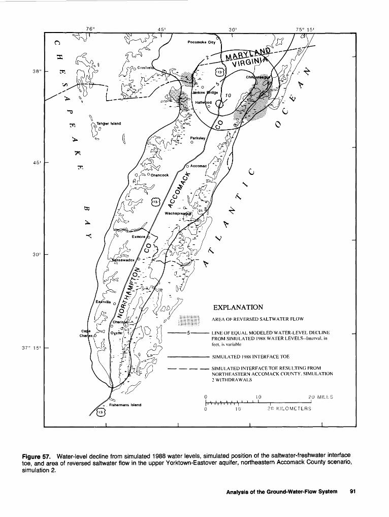
76° 45' 30' 75° 15'

45'

30'

37" 15'

EXPLANATION


LINE OF EQUAL MODELED WATER-LEVEL DECLINE FROM SIMULATED 1988 WATER LEVELS-Interval, in feet, is variable


SIMULATED INTERFACE TOE RESULTING FROM NORTHEASTERN ACCOMACK COUNTY, SIMULATION 2 WITHDRAWALS

20 MILLS

20 KILOMCTLRS

Figure 57. Water-level decline from simulated 1988 water levels, simulated position of the saltwater-freshwater interface toe, and area of reversed saltwater flow in the upper Yorktown-Eastover aquifer, northeastern Accomack County scenario, simulation 2.


76 C 45' 30' 75° 15'

38 C

45'

30'

37° 15'

EXPLANATION

LINE OF EQUAL MODELED WATER-LEVEL DECLINE FROM SIMULATED 1988 WATER LEVELS-lnterval, in feet, is variable



10 i i I

20 MILES

20 KILOMETERS

Figure 58. Water-level decline from simulated 1988 water levels and simulated position of the saltwater-freshwater inter face toe in the middle Yorktown-Eastover aquifer, northeastern Accomack County scenario, simulation 2.


75° 15'

EXPLANATION

UNE OF EQUAL MODELED WATER-LEVEL DECLINE FROM SIMULATED 1988 WATER LEVELS--Interval, in feet, is variable


20 KILOMETERS

37° 15" -

Figure 59. Water-level decline from simulated 1988 water levels and simulated position of the saltwater-freshwater inter face toe in the lower Yorktown-Eastover aquifer, northeastern Accomack County scenario, simulation 2.


Table 22. Permitted withdrawals as of January 1, 1990[Latitude and longitude are reported in degrees, arc minutes, arc seconds; Mgal/d, million gallons per day]

Map number 1

123456789101112131415161718192021222324

Facility

Accomack Nursing HomeAmerican OriginalBayshore ConcreteByrd FoodsC&D SeafoodCustis EnterprisesDicanioDicanioDicanioDicanioEastern Shore SeafoodExmore FoodsHolly FarmsJWTaylor PackingKMCFoodNASA, Wallops IslandNASA, main baseNew Church EnergyPeaceful BeachPerdueH. Alien SmithTown of Cape CharlesTown of ChincoteagueTown of Exmore

Latitude

37452837304537154037453037171137215037 13 3637 13 1437 13 5337 13 5437512137320137525637523937174637513437562637582337310537442937 17 15371605375626373231

Longitude

07537210754828076012107540100755524075552207600190760021075592307559080753337075 49 160753324075 35 270755728075304107528440753213075565007539200755512076001907527230754914

Permitted withdrawal (MgaVd)

0.029.250.125.600.152.441.047.047.093.093300

2.0011.800.549

1.600.127.263336229

2.639.150260

1.340320


does in simulation 1. The maximum amount of landward movement is approximately 0.5 mi in each simulation. The movement of the interface in the middle Yorktown-Eastover aquifer is identical for both the no-flow and the constant-head simulations (figs. 55 and 58). The location of the saltwater- freshwater interface toe in simulation 2 remains unchanged from 1988 conditions for the lower Yorktown-Eastover aquifer.

Simulated water levels indicate several areas of reversed ground-water flow (fig. 57) where there is potential for induced downward vertical leakage of saltwater into the freshwater parts of the upper Yorktown-Eastover aquifer. A comparison with the area of reversed flow from simulation 1 (fig. 54) shows that simulation 2 identifies a smaller area of potential induced saltwater leakage. The area of reversed ground-water flow is smaller for simulation 2 than simulation 1 because the water-level decline is reduced as a result of the unlimited supply of water from the constant-head boundary. The results of simulation 2 indicate that, even when an infinite amount of water is allowed through the northern and

eastern boundaries, saltwater intrusion through downward vertical leakage is possible, given the hypothetical projected increase in ground-water withdrawal in northeastern Accomack County.

Permitted-Withdrawal Scenario

The final scenario presented in this report examines the ground-water-flow system's response to currently (1990) permitted withdrawals. In 1976, the State of Virginia established Accomack and Northampton Counties as a Ground-Water Manage ment Area. Thus, all nonagricultural ground-water users withdrawing more than 300,000 gal/month must obtain a permit from the VWCB. As of 1990, most of the permitted ground-water users on the Eastern Shore were withdrawing less water than their permits allowed. In this scenario, ground-water conditions are simulated that would result from increasing withdrawal on the Eastern Shore to 1990 permitted levels.

Permitted withdrawal amounts as of Janu ary 1, 1990, ranged from 0.029 to 2.639 Mgal/d (table 22). Permitted withdrawals are widely spread


over the northern and southern ends of the peninsula (fig. 60). Withdrawals for ground-water users that do not have permits were continued at 1988 rates. Pumpage for the permitted scenario (13.824 Mgal/d) represents a 173 percent increase (8.763 Mgal/d) over 1988 withdrawals (table 18). Simulated 1988 conditions were used as initial conditions for a 100- year transient simulation of 1990 permitted with drawals. Although water levels respond quickly to changes in stress, the movement of the saltwater- freshwater interface takes place over long periods of time. The simulation was carried out to 100 years to provide insight into the long-term effects of increased withdrawals on the movement of the saltwater-freshwater interface.

Modeled water-level decline from simulated 1988 water levels is shown in figures 61-63. Water- level declines exceed 25 ft in the upper Yorktown- Eastover aquifers and 65 ft in the middle and lower Yorktown-Eastover aquifers. A maximum water- level decline of approximately 95 ft occurs in the middle Yorktown-Eastover aquifer near the town of Exmore (table 19). Water levels remain above the tops of the aquifers, indicating from a regional per spective that dewatering would be minimal at permitted-withdrawal levels.

The permitted-withdrawal scenario involves a greater increase in withdrawals over 1988 pumpage than any of the previous scenarios; therefore, the changes in the flow into and out of the confined system are the most dramatic (table 16). The increase in freshwater withdrawals of 8.65 Mgal/d over 1988 amounts results in an increase in flow into the confined-aquifer system by 4.33 Mgal/d and a decrease in natural flow out of the confined- aquifer system by 2.99 Mgal/d.

The position of the simulated saltwater- freshwater interface for the 100-year transient permitted-withdrawal scenario is shown in figures 61-63. Interface movement coincides with the areas of greatest water-level decline due to increased pumpage. Maximum inland movement of the saltwater-freshwater interface toe is approximately Imi in the upper Yorktown-Eastover aquifer near the town of Cape Charles and in the middle Yorktown-Eastover aquifer near the town of Chin- coteague. Maximum inland movement of the inter face toe is approximately 1 mi in the lower Yorktown-Eastover aquifer near the town of Hall- wood. The water-quality effects on the width of the mixing zone between saltwater and freshwater can

not be simulated by the sharp-interface model. The chloride concentrations in the mixing zone probably fluctuate more rapidly than the position of the sharp interface.

Water-level declines caused by pumpage in nearshore and coastal areas indicate several areas of reversed ground-water flow from the Atlantic Ocean and Chesapeake Bay to the freshwater parts of the upper Yorktown-Eastover aquifer (fig. 61). The areas of reversed flow indicate a potential for verti cal leakage of saltwater into the freshwater parts of the upper Yorktown-Eastover aquifer. The rate of vertical leakage of saltwater is highly dependent on the vertical hydraulic conductivity of the upper Yorktown-Eastover confining unit in the vicinity of the flow reversal.

Discussion of Model Results

The model results from the three scenarios of increased ground-water withdrawals provide infor mation on the regional response of the ground-water system to additional stress and its ability to meet future water needs. The simulations are not intended to predict exact ground-water conditions in the future; however, a comparison of model results pro vides useful information for the evaluation of alter native withdrawal scenarios.

The distribution of ground-water withdrawals directly affects the ability of the ground-water sys tem to sustain increased withdrawals without incur ring saltwater intrusion. An increase in ground-water withdrawals lowers ground-water levels around the pumping centers. Ground-water flow is diverted to the major pumping centers; water from adjacent parts of the aquifer and from adjacent aquifers or confining units replaces the water withdrawn. Large water-level declines could necessitate lowering of pump intakes, could increase the rate of movement of the offshore interface between saltwater and freshwater, and could induce leakage of poor-quality water from adjacent aquifers or surface-water bod ies. Excessive head declines and detrimental effects on water quality can be minimized with proper well placement. Withdrawal wells can be placed in areas that would minimize interference with other major ground-water users.

Any increase in withdrawals from the confined freshwater aquifers on the Eastern Shore increases the amount of recharge to and decreases the amount of natural discharge from the confined-aquifer system


76° 45' 30' 75° 15'

38'

45'

30'

37° 15'EXPLANATION

.12 LOCATION OF PERMITTED WITHDRAWAL AND IDENTIFIER

10 i i I

20 MILES

10 20 KILOMETERS

Figure 60. Location of permitted withdrawals.


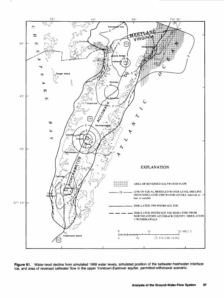
76"45

45' -

30' -

37" 15' -

EXPLANATION

Illlll AREA OF REVERSED SALTWATER FLOW

75 ____ LINE OF EQUAL MODELED WATER-LEVEL DECLINEFROM SIMULATED 1988 WATER LEVELS-Interval, in - feet, is variable



10 20 MILLS

?0 KILOMETERS

Figure 61. Water-level decline from simulated 1988 water levels, simulated position of the saltwater-freshwater interface toe, and area of reversed saltwater flow in the upper Yorktown-Eastover aquifer, permitted-withdrawal scenario.


76 C 45' 30' 75° 15'

38°

45'

30'

37° 15'

EXPLANATION

5 LINE OF EQUAL MODELED WATER-LEVEL DECLINE FROM SIMULATED 1988 WATER LEVELS-Interval, in feet, is variable


SIMULATED INTERFACE TOE RESULTING FROM PERMITTED-WITHDRAWAL SCENARIO

20 MILES

Fishermans Island10 20 KILOMETERS

Figure 62. Water-level decline from simulated 1988 water levels and simulated position of the saltwater-freshwater interface toe in the middle Yorktown-Eastover aquifer, permitted-withdrawal scenario.


76 C 45' 30' 75° 15'

38 C

45'

30'

37° 15'

EXPLANATION

5_____ LINE OF EQUAL MODELED WATER-LEVEL DECLINE FROM SIMULATED 1988 WATER LEVELS-Interval, in feet, is variable


SIMULATED INTERFACE TOE RESULTING FROM PERMITTED-W1THDRAWAL SCENARIO

10 i_I

20 MILES _I

20 KILOMETERS

Figure 63. Water-level decline from simulated 1988 water levels and simulated position of the saltwater-freshwater interface toe in the lower Yorktown-Eastover aquifer, permitted-withdrawal scenario.


A reduction in freshwater discharge to the Chesa peake Bay and Atlantic Ocean changes the equilib rium between the freshwater and the surrounding saltwater. The interface between freshwater and salt water begins to move inland as saltwater replaces the withdrawn freshwater. A reduction in freshwater discharge also could affect salinity levels at freshwater-discharge sites in nearshore inlets, bays, and estuaries.

Model results indicate that water-level declines in close proximity to the simulated location of the saltwater-freshwater interface have the most dra matic effect on the rate of interface movement. Large water-level declines in the center of the pen insula have a minimal effect on the rate of move ment of the saltwater-freshwater interface; however, small water-level declines in coastal areas adjacent to the interface position cause a noticeable increase in the rate of interface movement.

Two potential pathways for saltwater intrusion into the freshwater aquifers of the Eastern Shore were examined in this report. Model simulations show saltwater intrusion through lateral movement of the saltwater-freshwater interface and through downward vertical leakage of saltwater in areas where a saltwater source overlies the freshwater part of the uppermost confined aquifer. Model simula tions indicate that lateral movement of the saltwater- freshwater interface is slow and takes place over long periods of time. However, a reversal of the ground-water-flow direction can take place in short timeframes and could result in induced vertical leak age of saltwater through the confining unit into the freshwater part of an aquifer. Areas of reversed flow of saltwater into freshwater areas are seen in sce nario results where heavy withdrawals are present in coastal areas and water-level declines extend offshore.

Sensitivity Analysis

Model-sensitivity analyses were conducted to examine the response of the calibrated model to changes in boundary conditions and estimated hydraulic characteristics. The model sensitivity to the northern no-flow boundary condition is illus trated in the section of this report describing simula tion 2 of the northeastern Accomack County sce nario. Model runs also were conducted to determine the sensitivity of the model to changes in the overly ing constant-head boundary. Increasing the overly

ing constant heads (that represent the water table) resulted in a slight increase in the heads in the simu lated confined aquifers. Correspondingly, decreasing the overlying constant heads resulted in lower heads in the simulated confined aquifers. The hydraulic property that dominates flow through the system is the vertical leakance of the uppermost confining unit, and as a result, the model is more sensitive to changes in confining-unit vertical leakance than it is to changes in the overlying constant heads. The results of the sensitivity analysis of the calibrated model to changes in horizontal hydraulic conductiv ity of aquifers and leakance of confining units are presented in this section. Sensitivity simulations were conducted by increasing or decreasing an indi vidual parameter while all other characteristics remained unchanged. The larger the resulting changes in water levels are, the more sensitive the model is to that parameter, and the smaller the change, the less sensitive the model is.

Withdrawal conditions from simulation 1 of the southern Northampton County scenario were used to examine the model's sensitivity to large increases in withdrawals. Variations in hydraulic characteristics were compared by simulating a 50-percent increase and decrease in hydraulic con ductivity and vertical leakance. Water-level differ ences that resulted from changing the calibrated hydraulic parameters are shown in figures 64-67. The maximum water-level changes for each aquifer for each sensitivity run (table 23) show that the model is most sensitive near major pumping areas. Generally, the water levels simulated by the model are more sensitive to decreases than they are to increases in hydraulic conductivity and vertical leak ance. The responses of the saltwater-freshwater interface to changes in hydraulic conductivity and vertical leakance were slow and not sensitive over the 50-year simulation period. Increasing hydraulic conductivity and decreasing vertical leakance result in an interface position that is slightly closer to the shore in a few locations than the calibrated-scenario interface position. Decreasing hydraulic conductivity and increasing vertical leakance result in an inter face position that is slightly farther offshore in a few locations than the calibrated scenario.

Model Limitations

The ground-water-flow model developed for the Eastern Shore is a tool that was used to assist in


76 C 45' 30' 75° 15'

38 C

45'

30'

37° 15' LINE OF EQUAL DIFFERENCE BETWEEN SENSITIVITY RUN AND CALIBRATED SOUTHERN NORTHAMPTON COUNTY SCENARIO, SIMULATION 1--Interval, in feet, is variable

10 20 MILES

20 KILOMETERS

Figure 64. Difference in simulated water levels resulting from a 50-percent increase in horizontal hydraulic conductivity for the southern Northampton County scenario simulation 1, upper Yorktown-Eastover aquifer.


76° 45' 30' 75° 15'

45'

30'

37° 15'EXPLANATION

LINE OF EQUAL DIFFERENCE BETWEEN SENSITIVITY RUN AND CALIBRATED SOUTHERN NORTHAMPTON COUNTY SCENARIO, SIMULATION 1--Interval, in feet, is variable

10 i_I

20 MILES _I

10 20 KILOMETERS

Figure 65. Difference in simulated water levels resulting from a 50-percent decrease in horizontal hydraulic conductivity for the southern Northampton County scenario simulation 1, upper Yorktown-Eastover aquifer.


76°

Jenkins Bridge

Hallwood

._ /"^Tangier Island

EXPLANATION


20 KILOMETERS

37° 15' -

Figure 66. Difference in simulated water levels resulting from a 50-percent increase in confining unit leakance for the southern Northampton County scenario simulation 1, upper Yorktown-Eastover aquifer.


76 C 45' 30' 75° 15'

38 C

45'

30'

37° 15'EXPLANATION


Island

0 10I.W.MM- ' ' '

20 MILES

20 KILOMETERS

I_______________I

Figure 67. Difference in simulated water levels resulting from a 50-percent decrease in confining unit leakance for the southern Northampton County scenario simulation 1, upper Yorktown-Eastover aquifer.


Table 23. Maximum water-level changes resulting from sensitivity runs

Maximum Grid location of increase Maximum Grid location of decreasewater-level _____________ water-level _____________increase Row Column decline Row Column(feet) (feet)

50-percent increase in hydraulic conductivityUpper Yorktown-EastoverMiddle Yorktown-EastoverLower Yorktown-Eastover

50-percent decrease in hvdraulic conductivityUpper Yorktown-EastoverMiddle Yorktown-EastoverLower Yorktown-Eastover

50-oercent increase in confining unit leakanceUpper Yorktown-EastoverMiddle Yorktown-EastoverLower Yorktown-Eastover

50-percent decrease in confining unit leakanceUpper Yorktown-EastoverMiddle Yorktown-EastoverLower Yorktown-Eastover

4.010.514.6

5.85.45.5

3.67.65.6

1.0.9

1.0

38080

434345

308080

516663

272926

282929

312926

393737

-3.5-33-32

-10.7-24.5-39.5

-1.5-23-3.0

-6.7-13.9-10.0

434545

38080

586057

298080

282829

272926

424340

332926

the analysis of the ground-water-flow system. The model is an approximate representation of a com plex physical system. The hydrogeologic character istics of a conceptualized three-dimensional system of aquifers and confining units are integrated in the model. Stresses can be applied to this quasi-three- dimensional representation of the system, and the relative effects of those stresses on the water levels, the water budget, and the saltwater-freshwater inter face can be examined.

The model was developed to simulate regional effects of hydrologic stresses on the ground-water- flow system. The large spatial and temporal scale of the model makes it unsuitable for the analysis of local effects, short-term effects, and small-scale withdrawals. A small-scale analysis of the flow system would require spatial and temporal refine ment of the aquifer and confining-unit characteristics and hydrologic stresses.

The model simulates ground-water flow in the Eastern Shore's freshwater-bearing confined aqui fers, from which the majority of withdrawals are made. The water table in the unconfined aquifer was specified in the model as a constant-head boundary to simulate the regional recharge-discharge relation between the unconfined aquifer and the confined

system, but flow in the unconfined aquifer was not simulated. The deep, saltwater aquifers (approxi mately 300 ft below land surface) also are not simu lated by the model. As of 1990, no water was being pumped from the deep aquifers in the study area.

The saltwater-freshwater interface is repre sented in the model as a sharp interface. There are no offshore data for the Eastern Shore; therefore, the actual position of the saltwater-freshwater inter face and the width of the transition zone are unknown. Saltwater and freshwater are simulated as immiscible fluids, and mixing due to hydrodynamic dispersion is neglected. Leakage between the salt water and freshwater zone is restricted by the model. Saltwater is not allowed to leak into the freshwater zone. The leakage of freshwater is dis tributed between the saltwater and freshwater zones based on the amounts of each type of water in the node receiving the leakage. The approach is designed to reproduce the general response of the interface and does not provide information concern ing the nature of the transition zone between salt water and freshwater. Vertical leakage of saltwater into freshwater is not directly simulated; evidence of vertical saltwater intrusion from overlying salty- surface-water bodies is provided by examination of


the water-level gradients and areas of reversed ground-water flow. The model is not able to simu late upconing of saltwater as a result of pumpage. This approach is considered an initial step in the process of characterizing the interactions between saltwater and freshwater around the Eastern Shore. Data concerning the dispersive properties of the sed iments and a solute-transport-modeling approach to the saltwater-freshwater interface are needed to fully characterize the water quality in the transition zone between saltwater and freshwater.

The location of the historical and present-day saltwater-freshwater interface is not known. The model simulates the location of the interface by sim ulating saltwater and freshwater flow and balancing pressures along the interface. The historic pre- stressed position of the interface is assumed, for the purposes of this report, to be in equilibrium with present-day sea levels. However, the interface posi tion may not have reached an equilibrium position and may still be responding to long-term sea-level fluctuations.

SUMMARY

The Eastern Shore of Virginia is totally dependent on ground water for its freshwater sup ply. Increased pumpage due to intensifying agricul tural, industrial, commercial, and urban develop ment could limit the continued use of this resource. Ground-water withdrawal has caused lowering of water levels and has created cones of depression around areas of heavy ground-water use. The water- level decline has resulted in well interference in sev eral localities. Continued water-level decline could result in additional well interference among the ground-water users and intrusion of saltwater into the freshwater parts of aquifers.

This report describes the hydrogeology and ground-water flow system of the Eastern Shore. A model that includes the ability to track the move ment of the saltwater-freshwater interface was used to aid in the hydrologic analysis of the effects of withdrawals on the ground-water-flow system.

The sediment of the Eastern Shore forms a layered sequence of aquifers and intervening confin ing units. This report focuses on the aquifers and confining units (approximately the upper 300 ft) that make up the fresh-ground-water system. The aqui fers that contain freshwater are the unconfined Columbia aquifer and the upper three confined aqui

fers, the upper, middle, and lower Yorktown- Eastover aquifers. Maps delineating the tops of the aquifers arM confining units were developed from correlation of lithologic and geophysical logs, water- quality analyses, and water-level data.

Prior to 1940, ground-water withdrawals on the Eastern Shore were minimal, and the ground- water system was in a state of long-term dynamic equilibrium. Water from precipitation falling on the peninsula recharged the Columbia aquifer and flowed from the topographic highs near the center of the peninsula to discharge into streams, estuaries, the Chesapeake Bay, and the Atlantic Ocean. Some water flowed vertically through the upper Yorktown- Eastover confining unit to recharge the confined- aquifer system. Water-level measurements made after withdrawals began on the peninsula indicated lowering of water levels and creation of cones of depression around major pumping centers.

Annual ground-water-withdrawal data for the model area were compiled by aquifer for commer cial, industrial, and municipal withdrawals. Prior to 1965, there were few large users of ground water on the Eastern Shore. By 1970, increased population along with commercial and industrial growth greatly increased the demand for the ground water. Ground- water use, excluding domestic and irrigation, was estimated to be about 5.04 Mgal/d in 1988. The upper, middle, and lower Yorktown-Eastover aqui fers supplied 36, 42, and 22 percent of the 5.039 Mgal/d withdrawal, respectively. Major pumping centers on the Eastern Shore were located near the towns of Chincoteague, Hall wood, Accomac, Exmore, Oyster, Cheriton, and Cape Charles.

Data on chloride concentrations were compiled by aquifer to provide information on the distribution of chlorides in the study area. Chloride concentra tions in each aquifer are typically lower in the mid dle of the peninsula than they are along the coast. Chloride concentrations increase with depth and are higher in the lower Yorktown-Eastover aquifer than in the middle and upper Yorktown-Eastover aqui fers. The elevated chloride concentrations (greater than 250 mg/L) found in the lower Yorktown- Eastover aquifer across the peninsula near Exmore, Va., could be a result of different hydraulic proper ties related to the presence of an ancient Pleistocene river channel. Chloride concentrations in the lower Yorktown-Eastover aquifer are stratified, and con centrations are lower near the top than near the bot tom of the aquifer.


A model was developed for the Eastern Shore to simulate changes in ground-water-flow conditions that result from changes in hydrologic stresses. Sim ulation included ground-water flow both prior to ground-water pumpage and throughout the history of pumpage. The maximum simulated water-level decline since prepumping conditions was 53 ft in the lower Yorktown-Eastover aquifer near the town of Accomac, Va. Simulated water-level gradients indi cated a change in the direction of ground-water flow from prepumping conditions. Prepumping flow was from topographic highs in the center of the penin sula to the Chesapeake Bay and Atlantic Ocean. Simulated 1988 conditions show ground-water flow is being diverted toward the major pumping centers. Ground-water pumpage is supplied by an increase in vertical leakage to the confined-aquifer system from the unconfined aquifer and a decrease in vertical leakage from the confined-aquifer system to the unconfined aquifer. The simulated position of the interface between saltwater and freshwater did not change in response to historic pumpage.

Three scenarios predicted ground-water condi tions that result from increasing withdrawals in southern Northampton County, in northeastern Accomack County, and throughout the peninsula at 1990 permitted rates. Simulation results indicate that water levels continue to decline as withdrawals increase and could result in well interference among major ground-water users and in a reduction in freshwater discharge to the Chesapeake Bay and Atlantic Ocean. The water-level declines associated with the increased withdrawals could cause slight movement of the saltwater-freshwater interface over a 50-year simulation period. The potential for induced vertical leakage of saltwater from overlying salty-surface-water sources into the freshwater parts of the upper Yorktown-Eastover aquifer is indicated by areas of reversed ground-water gradients caused by offshore water-level declines.

REFERENCES CITED

Back, William, 1966, Hydrochemical facies and ground- water flow patterns in the northern part of the Atlan tic Coastal Plain: U.S. Geological Survey Profes sional Paper 498-A, 42 p.

Bal, G.P., 1977, Computer simulation model for ground- water flow in the Eastern Shore of Virginia: Virginia State Water Control Board Planning Bulletin 309, 73 p.

Bear, Jacob, 1979, Hydraulics of ground water: New York, McGraw-Hill, 569 p.

Bond, L.D., and Bredehoeft, J.D., 1987, Origins of seawater intrusion in a coastal aquifer a case study of the Pajaro Valley: Journal of Hydrology, v. 92, p. 363-388.

Cederstrom, D.J., 1945, Geology and ground-water resources of the Coastal Plain in southeastern Vir ginia: Virginia Geological Survey Bulletin 63, 384 p.

Colman, S.M., Halka, J.P., Hobbs, C.H., Mixon, R.B., and Foster, D.S., 1990, Ancient channels of the Susquehanna River beneath the Chesapeake Bay and the Delmarva Peninsula: Geological Society of America Bulletin, v. 102, p. 1268-1279.

Colman, S.M., and Mixon, R.B., 1988, The record of major Quaternary sea-level fluctuations in a large Coastal Plain estuary, Chesapeake Bay, eastern United States: Palaeogeography, Palaeoclimatology, and Palaeoecology, v. 68, p. 99-116.

Cooper, H.H., Jr., 1959, A hypothesis concerning the dynamic balance of freshwater and saltwater in a coastal aquifer: Journal of Geophysical Research, v. 64, no. 4, p. 461-467.

Cooper, H.H., Jr., and Jacob, C.E., 1946, A generalized graphical method for evaluating formation constants and summarizing well-field history: American Geophysical Union Transactions, v. 27, no. 4, p. 526-534.

Gushing, E.M., Kantrowitz, I.H., and Taylor, K.R., 1973, Water resources of the Delmarva Peninsula: U.S. Geological Survey Professional Paper 822, 58 p.

Essaid, H.I., 1986, A comparison of the coupledfreshwater-saltwater flow and the Ghyben-Herzberg sharp interface approaches to modeling of transient behavior in coastal aquifer systems: Journal of Hydrology, v. 86, p. 169-196.

1990a, The computer model, SHARP, a quasi- three-dimensional finite-difference model to simulate freshwater and saltwater flow in layered coastal aqui fer systems: U.S. Geological Survey Water- Resources Investigations Report 90-4130, 181 p.

-1990b, A multilayered sharp interface model ofcoupled freshwater and saltwater flow in coastal sys tems model development and application: Water Resources Research, v. 26, no. 7, p. 1431-1454.

Fennema, R.J., and Newton, V.P., 1982, Ground water resources of the Eastern Shore of Virginia: Virginia State Water Control Board Planning Bulletin 322, 94 p.

Glaser, J.D., 1969, Petrology and origin of Potomac and Magothy (Cretaceous) sediments, middle Atlantic Coastal Plain: Maryland Geological Survey Report of Investigations 11, 101 p.

References Cited 107

Hack, J.T., 1957, Submerged river system of Chesapeake Bay (Maryland-Virginia): Geological Society of America Bulletin, v. 68, no. 7, p. 817-830.

Hamilton, P.A., and Larson, J.D., 1988, Hydrogeology and analysis of the ground-water flow system in the Coastal Plain of southeastern Virginia: U.S. Geologi cal Survey Water-Resources Investigations Report 87^240, 175 p.

Hansen, H.J., 1969, Depositional environments of sub surface Potomac Group in southern Maryland: Amer ican Association of Petroleum Geologists Bulletin, v. 53, no. 9, p. 1923-1937.

Harsh, J.F., and Laczniak, R.J., 1986, Conceptualization and analysis of the ground-water system in the Coastal Plain aquifers of Virginia: U.S. Geological Survey Professional Paper 1404-E, 107 p.

Heath, Ralph C., 1983, Basic ground-water hydrology: U.S. Geological Survey Water-Supply Paper 2220, 84 p.

Hill, M.C., 1988, A comparison of coupled freshwater- saltwater sharp-interface and convective-dispersive models of saltwater intrusion in a layered aquifer system, in Proceedings of the VII International Con ference on Computational Methods in Water Resources: New York, Elsevier, p. 211-216.

Knobel, L.L., 1985, Ground-water-quality data for the Atlantic Coastal Plain: New Jersey, Delaware, Mary land, Virginia, and North Carolina: U.S. Geological Survey Open-File Report 85-154, 84 p.

Kohout, F.E., 1964, The flow of freshwater and saltwater in the Biscayne aquifer in the Miami area, Florida Seawater in coastal aquifers: U.S. Geological Survey Water-Supply Paper 1613-C, p. C12-C32.

Kull, T.K., and Laczniak, R.J., 1987, Ground-water withdrawals from the confined aquifers in the Coastal Plain of Virginia, 1891-1983: U.S. Geologi cal Survey Water-Resources Investigations Report 87-4049, 37 p.

Laczniak, R.J., and Meng, A.A., HI, 1988, Ground- water resources of the York-James Peninsula of Virginia: U.S. Geological Survey Water-Resources Investigations Report 88^059, 178 p.

Larson, J.D., 1981, Distribution of saltwater in the Coastal Plain aquifers of Virginia: U.S. Geological Survey Open-File Report 81-1013, 25 p.

Lohman, S.W., 1979, Ground-water hydraulics: U.S. Geological Survey Professional Paper 708, 70 p.

Meisler, Harold, Leahy, P.P., and Knobel, L.L., 1985, Effect of eustatic sea-level changes on saltwater- freshwater relations in the northern Atlantic Coastal Plain: U.S. Geological Survey Water-Supply Paper 2255, 28 p.

Meng, A.A., Ill, and Harsh, J.F., 1988, Hydrogeologic framework of the Virginia Coastal Plain: U.S. Geo logical Survey Professional Paper 1404-C, 82 p.

Mixon, R.B., 1985, Stratigraphic and geomorphic frame work of uppermost Cenozoic deposits in the southern Delmarva Peninsula, Virginia and Maryland: U.S. Geological Survey Professional Paper 1067-G, 53 p.

Robbins, E.I., Perry, W.J., Jr., and Doyle, J.A., 1975, Palynological and Stratigraphic investigations of four deep wells in the Salisbury Embayment of the Atlan tic Coastal Plain: U.S. Geological Survey Open-File Report 75-307, 120 p.

Sanford, Samuel, 1913, The underground water resources of the Coastal Plain province of Virginia: Virginia Geological Survey Bulletin 5, 361 p.

Sinnott, Alien, and Tibbitts, G.C., Jr., 1954, Summary of geology and ground-water resources of the East ern Shore Peninsula, Virginia a preliminary report: Virginia Division of Mineral Resources Circular 2, 18 p.

1957, Subsurface correlations based on selected well logs from the Eastern Shore Peninsula, Vir ginia: Virginia Division of Mineral Resources Circu lar 6, 11 p.

1968, Ground-water resources of Accomack andNorthampton Counties, Virginia: Virginia Division of Mineral Resources, Mineral Resources Report 9, 113 p.

Siudyla, E.A., 1975, Ground water conditions in theEastern Shore of Virginia: Virginia State Water Con trol Board Planning Bulletin 45 and Supplement, 20 p.

Siudyla, E.A., Berglund, T.D., and Newton, V.P., 1977, Ground water of the Middle Peninsula, Virginia: Virginia State Water Control Board Planning Bulle tin 305, 45 p.

Siudyla, E.A., May, A.E., and Hawthorne, D.W., 1981, Ground water resources of the Four Cities area, Vir ginia: Virginia Water Control Board Planning Bulle tin 331, 168 p.

Theis, C.V., 1935, The relation between the lowering of the piezometric surface and the rate and duration of discharge of a well using ground-water storage: American Geophysical Union Transactions, v. 16, p. 510-524.

U.S. Environmental Protection Agency, 1989, Proposed rule, National primary and secondary drinking water regulations: U.S. Federal Register, v. 54, no. 97, May 22, 1989, p. 22, 160.

Volker, R., and Rushton, K., 1982, An assessment of the importance of some parameters for seawater intru sion in aquifers and a comparison of dispersive and sharp-interface modelling approaches: Journal of Hydrology, v. 56, p. 239-250.

Werkheiser, W.H., 1990, Hydrogeology and ground- water resources of Somerset County, Maryland: Maryland Geological Survey Bulletin 35, 156 p.


hydrogeology and analysis of the ground-water-flow … · hydrogeology and analysis of the...

Documents