hydroelastic analysis of flexible floating interconnected structures_2
DESCRIPTION
HydroelasticTRANSCRIPT
ARTICLE IN PRESS
0029-8018/$ - see
doi:10.1016/j.oc
�CorrespondiNorwegian Uni
Norway. Tel.: +
E-mail addre
Ocean Engineering 34 (2007) 1516–1531
www.elsevier.com/locate/oceaneng
Hydroelastic analysis of flexible floating interconnected structures
Shixiao Fua,b,�, Torgeir Moana, Xujun Chena, Weicheng Cuib,c
aCentre for Ships and Ocean Structures, Norwegian University of Science and Technology, N-7491 Trondheim, NorwaybSchool of Naval Architecture, Ocean and Civil Engineering, Shanghai Jiao Tong University, Shanghai 200030, China
cChina Ship Scientific Research Center, Wuxi 214082, China
Received 6 November 2006; accepted 9 January 2007
Available online 3 February 2007
Abstract
Three-dimensional hydroelasticity theory is used to predict the hydroelastic response of flexible floating interconnected structures. The
theory is extended to take into account hinge rigid modes, which are calculated from a numerical analysis of the structure based on the
finite element method. The modules and connectors are all considered to be flexible, with variable translational and rotational connector
stiffness. As a special case, the response of a two-module interconnected structure with very high connector stiffness is found to compare
well to experimental results for an otherwise equivalent continuous structure. This model is used to study the general characteristics of
hydroelastic response in flexible floating interconnected structures, including their displacement and bending moments under various
conditions. The effects of connector and module stiffness on the hydroelastic response are also studied, to provide information regarding
the optimal design of such structures.
r 2007 Elsevier Ltd. All rights reserved.
Keywords: Interconnected structures; Hinge modes; Linear hydroelasticity; Frequency domain; Bending moment; Displacement
1. Introduction
Very large floating structures (VLFS) can be used for avariety of purposes, such as airports, bridges, storagefacilities, emergency bases, and terminals. A key feature ofthese flexible structures is the coupling between theirdeformation and the fluid field. A variety of VLFS hulldesigns have emerged, including monolithic hulls, semi-submersible hulls, and hulls composed of many intercon-nected flexible modules.
Various theories have been developed in order to predictthe hydroelastic response of continuous flexible structures.For simple spatial models such as beams and plates, one-,two- and three-dimensional hydroelasticity theories havebeen developed. Many variations of these theories havebeen adopted using both analytical formulations (Sahooet al., 2000; Sun et al., 2002; Ohkusu, 1998) and numerical
front matter r 2007 Elsevier Ltd. All rights reserved.
eaneng.2007.01.003
ng author. Centre for Ships and Ocean Structures,
versity of Science and Technology, N-7491 Trondheim,
47 73551108.
ss: [email protected] (S. Fu).
methods (Wu et al., 1995; Kim and Ertekin, 1998; Ertekinand Kim, 1999; Eatock Taylor and Ohkusu, 2000; EatockTaylor, 2003; Cui et al., 2007). Specific hydrodynamicformulations based on the modal representation ofstructural behaviour, traditional three-dimensional sea-keeping theory, and linear potential theory have beendeveloped to predict the response of both beam-likestructures (Bishop and Price, 1979) and those of arbitraryshape (Wu, 1984), through application of two-dimensionalstrip theory and the three-dimensional Green’s functionmethod, respectively. Other hydroelastic formulations alsoexist based upon two-dimensional (Wu and Moan, 1996;Xia et al., 1998) and three-dimensional nonlinear theory(Chen et al., 2003a). Finally, several hybrid methods ofhydroelastic analysis for the single module problem havealso been developed (Hamamoto, 1998; Seto and Ochi,1998; Kashiwagi, 1998; Hermans, 1998).To predict the hydroelastic response of interconnected
multi-module structures, multi-body hydrodynamic inter-action theory is usually adopted. In this theory, bothmodules and connectors may be modelled as either rigid orflexible. There are, therefore, four types of model: Rigid
ARTICLE IN PRESSS. Fu et al. / Ocean Engineering 34 (2007) 1516–1531 1517
Module and Rigid Connector (RMRC), Rigid Module andFlexible Connector (RMFC), Flexible Module and RigidConnector (FMRC) and Flexible Module and FlexibleConnector (FMFC). By adopting two-dimensional linearstrip theory, ignoring the hydrodynamic interactionbetween modules, and using a simplified beam model withvarying shear and flexural rigidities, Che et al. (1992)analysed the hydroelastic response of a 5-module VLFS.Che et al. (1994) later extended this theory by representingthe structure with a three-dimensional finite element modelrather than as a beam. Various three-dimensional methods(in both hydrodynamics and structural analysis) have beendeveloped using source distribution methods to analyseRMFC models (Wang et al., 1991; Riggs and Ertekin,1993; Riggs et al., 1999; Cui et al., 2007). These formu-lations account for the hydrodynamic interactions betweeneach module by considering the radiation conditionscorresponding to the motion of each module in one ofits six rigid modes, while keeping the other modulesfixed. By employing the composite singularity distributionmethod and three-dimensional hydroelasticity theory,Wu et al. (1993) analysed the hydroelastic response of a5-module VLFS with FMFC. Riggs et al. (2000) com-pared the wave-induced response of an interconnectedVLFS under the RMFC and FMFC (FEA) models.They found that the effect of module elasticity in theFMFC model could be reproduced in a RMFC model bychanging the stiffness of the RMFC connectors to matchthe natural frequencies and mode shapes of the twomodels.
The methods considered so far deal with modules joinedby connectors at both deck and bottom levels, so that thereis no hinge modes existed, or all the modules are consideredto be rigid. In a structure composed of serially andlongitudinally connected barges, Newman (1997a, b,1998a) explicitly defined hinge rigid body modes torepresent the relative motions between the modules andthe shear force loads in the connectors (WAMIT; Lee andNewman, 2004). In addition to accounting for hingedconnectors, modules can be modelled as flexible beams(Newman, 1998b; Lee and Newman, 2000; Newman,2005). Using WAMIT and taking into account theelasticity of both modules and connectors, Kim et al.(1999) studied the hydroelastic response of a five-moduleVLFS in the linear frequency domain, where the elasticityof modules and connectors is modelled by using astructural three-dimensional FE modal analysis, and thehinge rigid modes are explicitly defined following Newman(1997a, b) and Lee and Newman (2004).
When it comes to the more complicated interconnectedmulti-body structures, composed of many flexible modulesthat need not be connected serially, it will become verydifficult to explicitly define the hinge modes of rigid relativemotion and shear force. In particular, it is difficult toensure that the orthogonality conditions of the hinge rigidmodes are satisfied with respect to the other flexible androtational rigid modes. The purpose of this paper is to
demonstrate a method of predicting the hydroelasticresponse of a flexible, floating, interconnected structureusing general three-dimensional hydroelasticity theory(Wu, 1984), extending previous work to take into accounthinge rigid modes. These modes are calculated through anumerical analysis of the structure based on the finiteelement method, rather than being explicitly defined tomeet orthogonality conditions. All the modules andconnectors are considered to be flexible. The translationaland rotational stiffness of the connectors is also consid-ered. This method is validated by a special numericalcase, where the hydroelastic response for very highconnector stiffness values is shown to be the equivalentto that of a continuous structure. Using the results ofthis test model, the hydroelastic responses of more generalstructures are studied, including their displacementand bending moments. Moreover, the effect of connectorand module stiffness on the hydroelastic response is studiedto provide insight into the optimal design of suchstructures.
2. Equations of motion for freely floating flexible structures
Using the finite element method, the equation of motionfor an arbitrary structural system can be represented as
½M�f €Ug þ ½C�f _Ug þ ½K �fUg ¼ fPg, (1)
where [M], [C] and [K] are the global mass, damping andstiffness matrices, respectively; {U} is the nodal displace-ment vector; and {P} is the vector of structural distributedforces. All of these entities are assembled from thecorresponding single element matrices [Me], [Ce], [Ke],{Ue}, and {Pe} using standard FEM procedures. Theconnectors are modeled by translational and rotationalsprings, and can be incorporated into the motion equationsusing standard FEM procedures.Neglecting all external forces and damping yields the free
vibration equation of the system:
½M�f €Ug þ ½K �fUg ¼ f0g. (2)
Assuming that Eq. (2) has a harmonic solution withfrequency o, this then leads to the following eigenvalueproblem:
ð�o2½M� þ ½K �ÞfDg ¼ f0g. (3)
Provided that [M] and [K] are symmetric and [M] ispositive definite, and that [K] is positive definite (for asystem without any free motions) or semi-definite (for asystem allowing some special free motions), all theeigenvalues of Eq. (3) will be non-negative and real. Theeigenvalues o2
r ðr ¼ 1; 2; 3; . . . ; 6nÞ represent the squarednatural frequencies of the system:
0po21po2
2 ; � � � ; po26n, (4)
where o2r40 when [K] is positive definite, and o2
rX0when [K] is semi-definite. Each eigenvalue is associatedwith a real eigenvector {Dr}, which represents the rth
ARTICLE IN PRESSS. Fu et al. / Ocean Engineering 34 (2007) 1516–15311518
natural mode:
fDrg ¼ ffDr1g; fDr2g ; . . . ; fDrjg ; . . . ; fDrnggT, (5)
where fDrig is the eigenvector of the ith node whichcontains 6 degree of freedoms, and i runs over the n nodesof the structural FE model system. fdrg, a sub-matrix offDrg, consists of the rth natural mode components of all thenodes associated with one particular element. The rthmodal shape {ur} at any point in that element can beexpressed as
u*
r ¼ ½l�T½N�½L�fdrg ¼ fur; vr;wrg
T, (6)
where [L] is a banded, local-to-global coordinate transformmatrix composed of diagonal sub-matrices [l], each ofwhich is a simple cosine matrix between two coordinates.[N] is the displacement interpolation function of thestructural element.
For freely floating, hinge-connected, multi-modulestructures, Eq. (3) has zero-valued roots corresponding tothe 6 modes of global rigid motion and the hinge modesdescribing relative motion between each module. Accord-ing to traditional seakeeping theory, the rigid modes of theglobal system can be described by three translationalcomponents (uG, vG, wG) and three rotational components(yxG, yyG, yzG) about the center of mass in the globalcoordinate system coincident with equilibrium. Thus, thefirst six rigid modes (with zero frequency) at any point j onthe freely floating body can be expressed by
fD1jg ¼ f 1; 0; 0; 0; 0; 0 gT;
fD2jg ¼ f 0; 1; 0; 0; 0; 0 gT;
fD3jg ¼ f 0; 0; 1; 0; 0; 0 gT;
fD4jg ¼ f 0; �ðz� zGÞ; ðy� yGÞ; 1; 0; 0 gT;
fD5jg ¼ f ðz� zGÞ; 0; �ðx� xGÞ; 0; 1; 0 gT;
fD6jg ¼ f� ðy� yGÞ; ðx� xGÞ; 0; 0; 0; 1 gT:
(7)
These vectors correspond to the six rigid motions of theglobal structure: surge, sway, heave, roll, pitch and yaw,where (x, y, z) and (xG, yG, zG) are the coordinates of apoint in the floating body and the center of mass,respectively. To obtain the zero-frequency hinge modesdescribing the relative motion between different modules,we transform the eigenvalue problem into a new one byintroducing an additional artificial stiffness proportional tothe mass, g[M] where g can be non-zero artificial realnumber close to the first non-zero eigenvalue of the system.Then we have
ð�l½M� þ ½K 0�ÞfX g ¼ f0g, (8)
where
l ¼ o2 þ g, (9)
½K 0� ¼ ½K � þ g½M�. (10)
From Eq. (8) we can get the corresponding positiveeigenvalues l and eigenvectors {X}. The orthogonality
conditions with respect to ½K� þ g½M� and [M] areautomatically satisfied in Eq. (8). Thus, these also cansatisfy the orthogonality conditions with respect to [K] and[M] for the original interconnected structure. This meansthat eigenvalues and eigenvectors of the original system cantherefore be expressed as
o2 ¼ l� g, (11)
fDrg ¼ fX rg. (12)
Since usually only the first several oscillatory modesdominate the structural dynamic response, we assume thatthe nodal displacement of the structure can written as asuperposition of the first m modes,
fUg ¼Xm
r¼1
fDrgprðtÞ ¼ ½D�fpg, (13)
where pr(t) refers to the rth generalized coordinate. Forr ¼ 1–6, {Dr} represents the vector of the first six rigidmodes and pr(t) the magnitude of rigid displacement aboutthe center of mass (xG, yG, zG). Substituting (13) into (1)and premultiplying by [D]T, the generalized equation ofmotion is as follows:
½a�f €pg þ ½b�f _pg þ ½c�fpg ¼ fZg, (14)
with
½a� ¼ ½D�T½M�½D�,
½b� ¼ ½D�T½C�½D�,
½c� ¼ ½D�T½K �½D�,
fZg ¼ ½D�TfPg ¼ fZ1;Z2 ; . . . ; Zmg. ð15Þ
[a], [b] and [c] are the generalized mass, damping andstiffness matrices respectively; {Z} is the generalizeddistributed force and can be expressed as
Zr ¼ �furgTfPg. (16)
In general, the generalized coordinates {p} in Eq. (14)separate naturally into two groups, which can be denotedby {pR} and {pD} respectively, that is to say
fpg ¼ fpR; pDgT, (17)
where
fpRg ¼ fp1; p2 ; . . . ; p6gT (18)
refers to the rigid body modes of the global structure asdefined by Eq. (7) and
fpDg ¼ fp7; p8 ; . . . ; pmgT (19)
refers to the distortion modes, including both rigid hingemodes and structural distortional modes. Eq. (14) can
ARTICLE IN PRESS
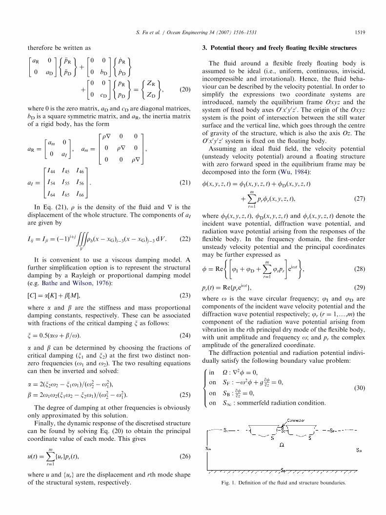
Fig. 1. Definition of the fluid and structure boundaries.
S. Fu et al. / Ocean Engineering 34 (2007) 1516–1531 1519
therefore be written as
aR 0
0 aD
" #€pR
€pD
( )þ
0 0
0 bD
" #_pR
_pD
( )
þ0 0
0 cD
" #pR
pD
( )¼
ZR
ZD
( ), ð20Þ
where 0 is the zero matrix, aD and cD are diagonal matrices,bD is a square symmetric matrix, and aR, the inertia matrixof a rigid body, has the form
aR ¼am 0
0 aI
" #; am ¼
rr 0 0
0 rr 0
0 0 rr
2664
3775,
aI ¼
I44 I45 I46
I54 I55 I56
I64 I65 I66
2664
3775. ð21Þ
In Eq. (21), r is the density of the fluid and r is thedisplacement of the whole structure. The components of aI
are given by
I ij ¼ I ji ¼ ð�1Þiþj
ZZZV
rbðx� xGÞi�3ðx� xGÞj�3 dV . (22)
It is convenient to use a viscous damping model. Afurther simplification option is to represent the structuraldamping by a Rayleigh or proportional damping model(e.g. Bathe and Wilson, 1976):
½C� ¼ a½K � þ b½M�, (23)
where a and b are the stiffness and mass proportionaldamping constants, respectively. These can be associatedwith fractions of the critical damping x as follows:
x ¼ 0:5ðaoþ b=oÞ. (24)
a and b can be determined by choosing the fractions ofcritical damping (x1 and x2) at the first two distinct non-zero frequencies (o1 and o2). The two resulting equationscan then be inverted and solved:
a ¼ 2ðx2o2 � x1o1Þ=ðo22 � o2
1Þ,
b ¼ 2o1o2ðx1o2 � x2o1Þ=ðo22 � o2
1Þ. ð25Þ
The degree of damping at other frequencies is obviouslyonly approximated by this solution.
Finally, the dynamic response of the discretised structurecan be found by solving Eq. (20) to obtain the principalcoordinate value of each mode. This gives
uðtÞ ¼Xm
r¼1
furgprðtÞ, (26)
where u and {ur} are the displacement and rth mode shapeof the structural system, respectively.
3. Potential theory and freely floating flexible structures
The fluid around a flexible freely floating body isassumed to be ideal (i.e., uniform, continuous, inviscid,incompressible and irrotational). Hence, the fluid beha-viour can be described by the velocity potential. In order tosimplify the expressions two coordinate systems areintroduced, namely the equilibrium frame Oxyz and thesystem of fixed body axes O0x0y0z0. The origin of the Oxyz
system is the point of intersection between the still watersurface and the vertical line, which goes through the centreof gravity of the structure, which is also the axis Oz. TheO0x0y0z0 system is fixed on the floating body.Assuming an ideal fluid field, the velocity potential
(unsteady velocity potential) around a floating structurewith zero forward speed in the equilibrium frame may bedecomposed into the form (Wu, 1984):
fðx; y; z; tÞ ¼ fIðx; y; z; tÞ þ fDðx; y; z; tÞ
þXm
r¼1
prfrðx; y; z; tÞ, ð27Þ
where fIðx; y; z; tÞ, fDðx; y; z; tÞ and frðx; y; z; tÞ denote theincident wave potential, diffraction wave potential, andradiation wave potential arising from the responses of theflexible body. In the frequency domain, the first-orderunsteady velocity potential and the principal coordinatesmay be further expressed as
f ¼ Re jI þ jD þXm
r¼1
jrpr
" #eiot
( ), (28)
prðtÞ ¼ Refpreiotg, (29)
where o is the wave circular frequency; jI and jD arecomponents of the incident wave velocity potential and thediffraction wave potential respectively; jr (r ¼ 1,y,m) thecomponent of the radiation wave potential arising fromvibration in the rth principal dry mode of the flexible body,with unit amplitude and frequency o; and pr the complexamplitude of the generalized coordinate.The diffraction potential and radiation potential indivi-
dually satisfy the following boundary value problem:
in O : r2f ¼ 0;
on SF : �o2fþ g qfqz¼ 0;
on SB :qfqz¼ 0;
on S1 : sommerfeld radiation condition:
8>>>><>>>>:
(30)
ARTICLE IN PRESSS. Fu et al. / Ocean Engineering 34 (2007) 1516–15311520
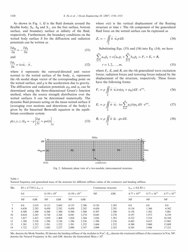
As shown in Fig. 1, O is the fluid domain around theflexible body; SF, SB and SN are the free surface, bottomsurface, and boundary surface at infinity of the fluid,respectively. Furthermore, the boundary conditions on thewetted body surface S for the diffraction and radiationpotentials can be written as
qfD
qn¼ �
qfI
qn(31)
and
qfr
qn¼ iou
*r � n
*, (32)
where n*
represents the outward-directed unit vectornormal to the wetted surface of the body, u
*r represents
the rth modal shape vector of the corresponding point onthe wetted surface, and g is the acceleration due to gravity.The diffraction and radiation potentials jD and jr can bedetermined using the three-dimensional Green’s functionmethod, where the source strength distribution over thewetted surfaces S can be determined numerically. Thedynamic fluid pressure acting on the mean wetted surface S
(averaging over motions and distortions of the body) isgiven by the linearised Bernoulli equation in the equili-brium coordinate system:
pðx; y; z; tÞjS ¼ �rqfqtþ gwðtÞ
� �S
. (33)
300
(0,0)
P1 P2 P3
P5
Fig. 2. Schematic plane view of a two
Table 1
Natural frequency and generalized mass of the structure for different stiffness
Mn. EI ¼ 4:77E11; krot ¼ C
0.0 0.159� 109 0.159� 1011 N
NF GM NF GM NF GM
7 0.0 2.619 0.115 2.602 0.155 2.308 0.
8 0.430 2.292 0.430 2.292 0.430 2.292 0.
9 0.500 1.500 0.500 1.500 0.500 1.500 0.
10 0.624 2.283 0.720 2.368 0.841 2.274 0.
11 1.017 1.412 1.019 1.404 1.024 1.384 1.
12 1.396 2.236 1.396 2.236 1.396 2.236 1.
13 1.581 1.252 1.581 1.252 1.581 1.252 1.
14 1.722 2.217 1.843 2.257 2.080 2.187 2.
Mn. denotes the Mode Number, EI denotes the bending stiffness of the modulu
denotes the Natural Frequency in Hz, and GM. denotes the Generalized Mas
where w(t) is the vertical displacement of the floatingstructure at time t. The rth component of the generalizedfluid force on the wetted surface can be expressed as
Zr ¼ �
ZZS
n*�u*
rpdS. (34)
Substituting Eqs. (33) and (34) into Eq. (14), we have
Xm
k¼1
ark €pk þ o2r arrpr þ
Xm
k¼1
brk _pk ¼ Fr þ Er þ Rr
r ¼ 1; 2; . . . ;m, ð35Þ
where Fr, Er and Rr are the rth generalized wave excitationforces, radiation forces and restoring forces induced by thedisplacement of the structure, respectively. These forceshave the following forms:
Fr ¼ rZZ
S
n*�u*
rioðjI þ jDÞdS � eiot, (36)
Er ¼ rZZ
S
n*�u*
r � ioXm
k¼1
pkðtÞjk dS � eiot, (37)
Rr ¼ rZZ
S
n*�ur � gwdS. (38)
60m
connectors
m
P4
-module, interconnected structure.
values of the connector and bending stiffness
ontinuous structure krot ¼ 0:0;EI ¼
F GM 4.77� 1010 4.77� 1012 4.77� 1013
NF NF NF
156 2.303 0.0 0.0 0.0
430 2.292 0.136 1.360 4.302
507 1.500 0.158 1.582 5.001
845 2.270 0.197 1.973 6.239
036 1.383 0.322 3.216 10.169
398 2.236 0.442 4.415 13.962
604 1.252 0.500 5.000 15.809
090 2.183 0.545 5.446 17.221
s in Nm2, Krot denotes the rotational stiffness of the connector in Nm, NF.
s� 106.
ARTICLE IN PRESSS. Fu et al. / Ocean Engineering 34 (2007) 1516–1531 1521
The restoring force can be expressed as
Rr ¼ �Xm
k¼1
pkCrkeiot (39)
with
Crk ¼ �rZZ
S
n*�u*
r � gwk dS, (40)
where the Crk are generalized restoring coefficients. When rp6and kp6, Eq. (40) reduces to the restoring coefficient matrix ofrigid motion. The other generalized coefficients can beobtained similarly. Placing all these coefficients into Eq. (14)yields the linear generalized hydroelastic equation of motion
ð½a� þ ½A�Þf €pg þ ð½b� þ ½B�Þf _pg þ ð½c� þ ½C�Þfpg ¼ fFg, (41)
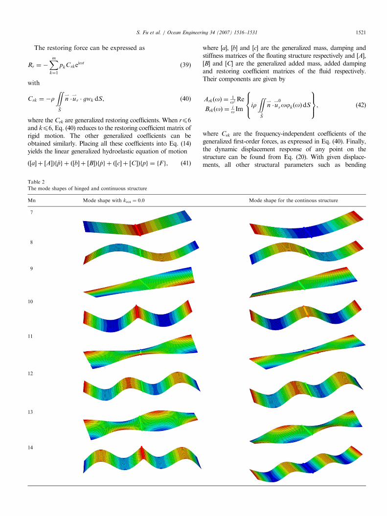
Table 2
The mode shapes of hinged and continuous structure
Mn Mode shape with krot ¼ 0.0
7
8
9
10
11
12
13
14
where [a], [b] and [c] are the generalized mass, damping andstiffness matrices of the floating structure respectively and [A],[B] and [C] are the generalized added mass, added dampingand restoring coefficient matrices of the fluid respectively.Their components are given by
ArkðoÞ ¼ 1o2 Re
BrkðoÞ ¼ io Im
irZZ
S
n*�u*0
rojkðoÞdS
8><>:
9>=>;, (42)
where Crk are the frequency-independent coefficients of thegeneralized first-order forces, as expressed in Eq. (40). Finally,the dynamic displacement response of any point on thestructure can be found from Eq. (20). With given displace-ments, all other structural parameters such as bending
Mode shape for the continous structure
ARTICLE IN PRESSS. Fu et al. / Ocean Engineering 34 (2007) 1516–15311522
moments, shearing forces, twisting moments and stresses canbe determined. For example, the bending moment at a certainsection of the structure becomes
MS ¼
I�DBkdls, (43)
where DB is the bending stiffness of the structure in a certaindirection, k is the curvature of structure deformation at agiven point in that direction (Chen et al., 2003b), and dlsis the length of the element included in the structure crosssection.
0.00.0 0.1 0.2 0.3 0.4 0
0.1
0.2
0.3
0.4
0.5
0.6
0.7
0.8
Vert
ical D
ispla
cem
ent
(w/A
)V
ert
ical D
ispla
cem
ent
(w/A
)V
ert
ical D
ispla
cem
ent (w
/A)
x
0.0 0.1 0.2 0.3 0.4 0
x
0.0 0.1 0.2 0.3 0.4
0.0
0.2
0.4
0.6
0.8
1.0
1.2
0.0
0.2
0.4
0.6
0.8
1.0
1.2
1.4
1.6
a
b
c
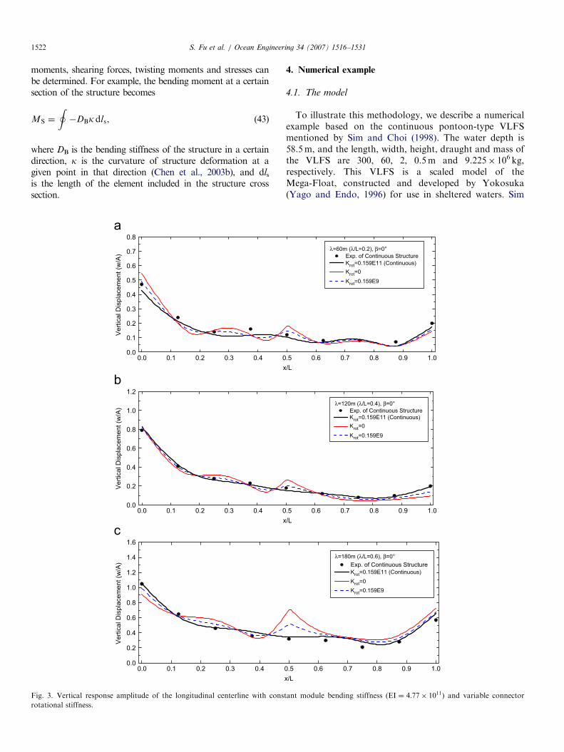
Fig. 3. Vertical response amplitude of the longitudinal centerline with cons
rotational stiffness.
4. Numerical example
4.1. The model
To illustrate this methodology, we describe a numericalexample based on the continuous pontoon-type VLFSmentioned by Sim and Choi (1998). The water depth is58.5m, and the length, width, height, draught and mass ofthe VLFS are 300, 60, 2, 0.5m and 9.225� 106 kg,respectively. This VLFS is a scaled model of theMega-Float, constructed and developed by Yokosuka(Yago and Endo, 1996) for use in sheltered waters. Sim
.5 0.6 0.7 0.8 0.9 1.0
λ=60m (λ/L=0.2), β=0°
Exp. of Continuous Structure
Krot=0.159E11 (Continuous)
Krot=0
Krot=0.159E9
Krot=0.159E11 (Continuous)
Krot=0
Krot=0.159E9
Krot=0.159E11 (Continuous)
Krot=0
Krot=0.159E9
/L
.5 0.6 0.7 0.8 0.9 1.0
/L
0.5 0.6 0.7 0.8 0.9 1.0
x/L
λ=120m (λ/L=0.4), β=0°
Exp. of Continuous Structure
λ=180m (λ/L=0.6), β=0°
Exp. of Continuous Structure
tant module bending stiffness (EI ¼ 4:77� 1011) and variable connector
ARTICLE IN PRESS
0.00.0 0.1 0.2 0.3 0.4 0.5 0.6 0.7 0.8 0.9 1.0
0.2
0.4
0.6
0.8
1.0
1.2
1.4
1.6
1.8
d
e
0.0
0.2
0.4
0.6
0.8
1.0
1.2
1.4
1.6
1.8
2.0
λ=240m (λ/L=0.8), β=0°
Exp. of Continuous Structure
Krot=0.159E11
Krot=0
Krot=0.159E9V
ert
ica
l D
isp
lace
me
nt (|
w|/A
)V
ert
ical D
ispla
cem
ent
(|w
|/A
)
x/L
0.0 0.1 0.2 0.3 0.4 0.5 0.6 0.7 0.8 0.9 1.0
x/L
λ=300m (λ/L=1.0), β=0°
Krot=0.159E11
Krot=0
Krot=0.159E9
Exp. of ContinuousStructure
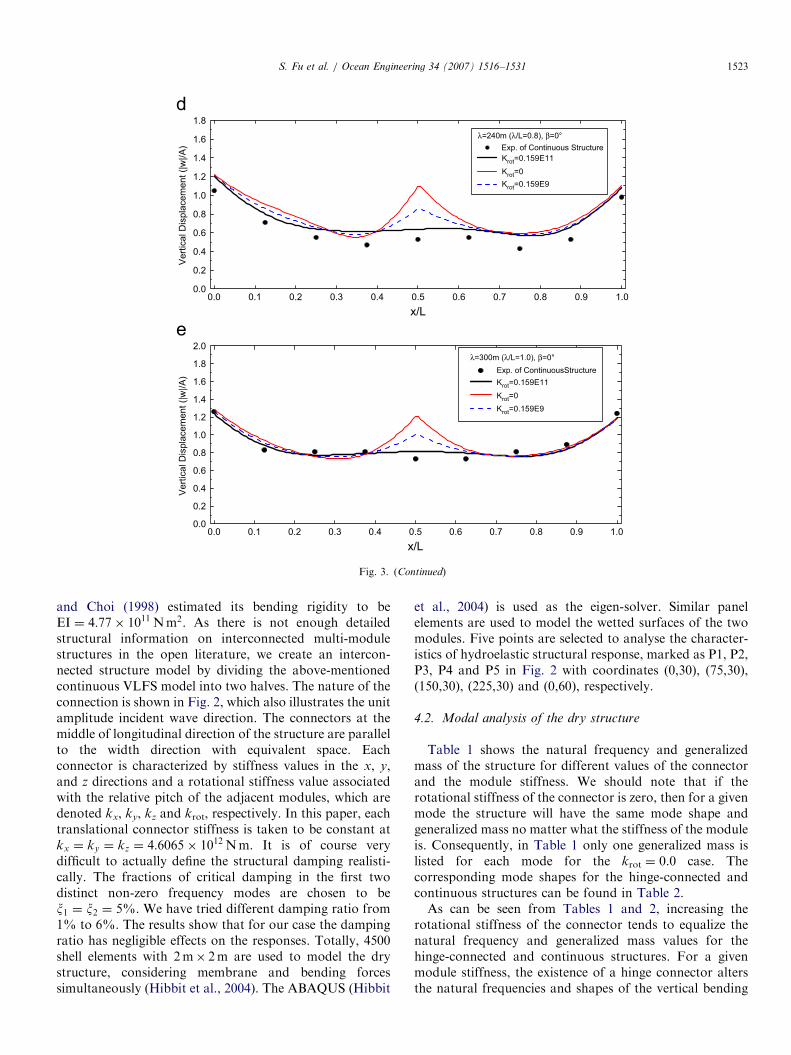
Fig. 3. (Continued)
S. Fu et al. / Ocean Engineering 34 (2007) 1516–1531 1523
and Choi (1998) estimated its bending rigidity to beEI ¼ 4:77� 1011 Nm2. As there is not enough detailedstructural information on interconnected multi-modulestructures in the open literature, we create an intercon-nected structure model by dividing the above-mentionedcontinuous VLFS model into two halves. The nature of theconnection is shown in Fig. 2, which also illustrates the unitamplitude incident wave direction. The connectors at themiddle of longitudinal direction of the structure are parallelto the width direction with equivalent space. Eachconnector is characterized by stiffness values in the x, y,and z directions and a rotational stiffness value associatedwith the relative pitch of the adjacent modules, which aredenoted kx, ky, kz and krot, respectively. In this paper, eachtranslational connector stiffness is taken to be constant atkx ¼ ky ¼ kz ¼ 4:6065� 1012 Nm. It is of course verydifficult to actually define the structural damping realisti-cally. The fractions of critical damping in the first twodistinct non-zero frequency modes are chosen to bex1 ¼ x2 ¼ 5%. We have tried different damping ratio from1% to 6%. The results show that for our case the dampingratio has negligible effects on the responses. Totally, 4500shell elements with 2m� 2m are used to model the drystructure, considering membrane and bending forcessimultaneously (Hibbit et al., 2004). The ABAQUS (Hibbit
et al., 2004) is used as the eigen-solver. Similar panelelements are used to model the wetted surfaces of the twomodules. Five points are selected to analyse the character-istics of hydroelastic structural response, marked as P1, P2,P3, P4 and P5 in Fig. 2 with coordinates (0,30), (75,30),(150,30), (225,30) and (0,60), respectively.
4.2. Modal analysis of the dry structure
Table 1 shows the natural frequency and generalizedmass of the structure for different values of the connectorand the module stiffness. We should note that if therotational stiffness of the connector is zero, then for a givenmode the structure will have the same mode shape andgeneralized mass no matter what the stiffness of the moduleis. Consequently, in Table 1 only one generalized mass islisted for each mode for the krot ¼ 0.0 case. Thecorresponding mode shapes for the hinge-connected andcontinuous structures can be found in Table 2.As can be seen from Tables 1 and 2, increasing the
rotational stiffness of the connector tends to equalize thenatural frequency and generalized mass values for thehinge-connected and continuous structures. For a givenmodule stiffness, the existence of a hinge connector altersthe natural frequencies and shapes of the vertical bending
ARTICLE IN PRESSS. Fu et al. / Ocean Engineering 34 (2007) 1516–15311524
modes more than for the torsional modes. Theoretically,the rotational stiffness of the connectors needs to approachinfinity for the interconnected and continuous structures tohave fully equivalent stiffness. These data show that for arotational stiffness of 0:159� 1011 Nm, however, thenatural frequencies and mode shapes of the interconnectedstructure are very close to the corresponding continuousvalues. The interconnected structure with a rotationalstiffness of 0:159� 1011 Nm can therefore be considered torespond similarly to the continuous structure. Unlessotherwise noted, in the following numerical results asuperposition of the first 35 modes is used in thehydroelastic analysis.
4.3. Numerical results
Fig. 3 shows the vertical displacement amplitude alongthe longitudinal centerline for experimental and numericalresults. The agreement between experimental and numer-ical results for the high-stiffness, ‘‘continuous’’ structure isgood. The corresponding validation for a continuousmodel has also been made by comparing the results ofthe present method, WAMIT and experiments (Taghipouret al., 2006). As there are no experimental results available
0.00.0 0.2 0.4 0.6 0.8 1
0.2
0.4
0.6
0.8
1.0
1.2
1.4
a
b
Vert
ical D
ispla
cem
ent
(|w
|/A
)
0.0
0.2
0.4
0.6
0.8
1.0
1.2
1.4
Vert
ical D
ispla
cem
ent (|
w|/A
)
Incident Wa
0.0 0.2 0.4 0.6 0.8 1
Incident Wave
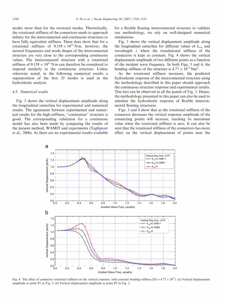
Fig. 4. The effect of connector rotational stiffness on the vertical response, wi
amplitude at point P1 in Fig. 2; (b) Vertical displacement amplitude at point
for a flexible floating interconnected structure to validateour methodology, we rely on well-designed numericalsimulations.Fig. 3 shows the vertical displacement amplitude along
the longitudinal centerline for different values of krot andwavelength l where the translational stiffness of theconnectors is kept as constant. Fig. 4 shows the verticaldisplacement amplitude of two different points as a functionof the incident wave frequency. In both Figs. 3 and 4, thebending stiffness of the structure is 4:77� 1011 Nm2.As the rotational stiffness increases, the predicted
hydroelastic response of the interconnected structure usingthe methodology described in this paper should approachthe continuous structure response and experimental results.This fact can be observed in all the panels of Fig. 3. Hence,the methodology presented in this paper can also be used tosimulate the hydroelastic response of flexible intercon-nected floating structures.Figs. 3 and 4 show that as the rotational stiffness of the
connector decreases the vertical response amplitude of theconnecting points will increase, reaching its maximumvalue when the rotational stiffness is zero. It can also beseen that the rotational stiffness of the connectors has moreeffect on the vertical displacement of points near the
.0 1.2 1.4 1.6 1.8 2.0
Vertical Disp.Amp. of P1
Krot=0.159E11
Krot=0.159E9
Krot=0
ve Freq. ω(rad/s)
.0 1.2 1.4 1.6 1.8 2.0
Freq. ω(rad/s)
Vertical Disp.Amp. of P3
Krot=0.159E11
Krot=0.159E9
Krot=0
th constant bending stiffness (EI ¼ 4:77� 1011). (a) Vertical displacement
P3 in Fig. 2.
ARTICLE IN PRESSS. Fu et al. / Ocean Engineering 34 (2007) 1516–1531 1525
connectors than on other positions. Moreover, the verticalresponse amplitude on the upstream side of the structure isalways larger than that on the downstream side.
The dynamic response of the fully hinged structure(when the rotational stiffness of the connectors is zero) willbe very different from that of the continuous structure. Thehinge connectors increase the vertical displacement ofconnecting points beyond the wave amplitude, a phenom-enon, which is never experienced in a continuous structure.
0.0
0.2
0.4
0.6
0.8
1.0
1.2
1.4
1.6
1.8
a
b
c
0.0
0.2
0.4
0.6
0.8
1.0
1.2
1.4
1.6
1.8
Vert
ical D
ispla
cem
en
t (|
w|/A
)V
ert
ical D
ispla
cem
ent
(|w
|/A
)V
ert
ical D
ispla
cem
ent (|
w|/A
)
0.00.0 0.2 0.4 0.6 0.8 1.0
0.2
0.4
0.6
0.8
1.0
1.2
1.4
1.6
Incident Wave
0.0 0.2 0.4 0.6 0.8 1.0
Incident Wave
0.0 0.2 0.4 0.6 0.8 1.0
Incident Wav
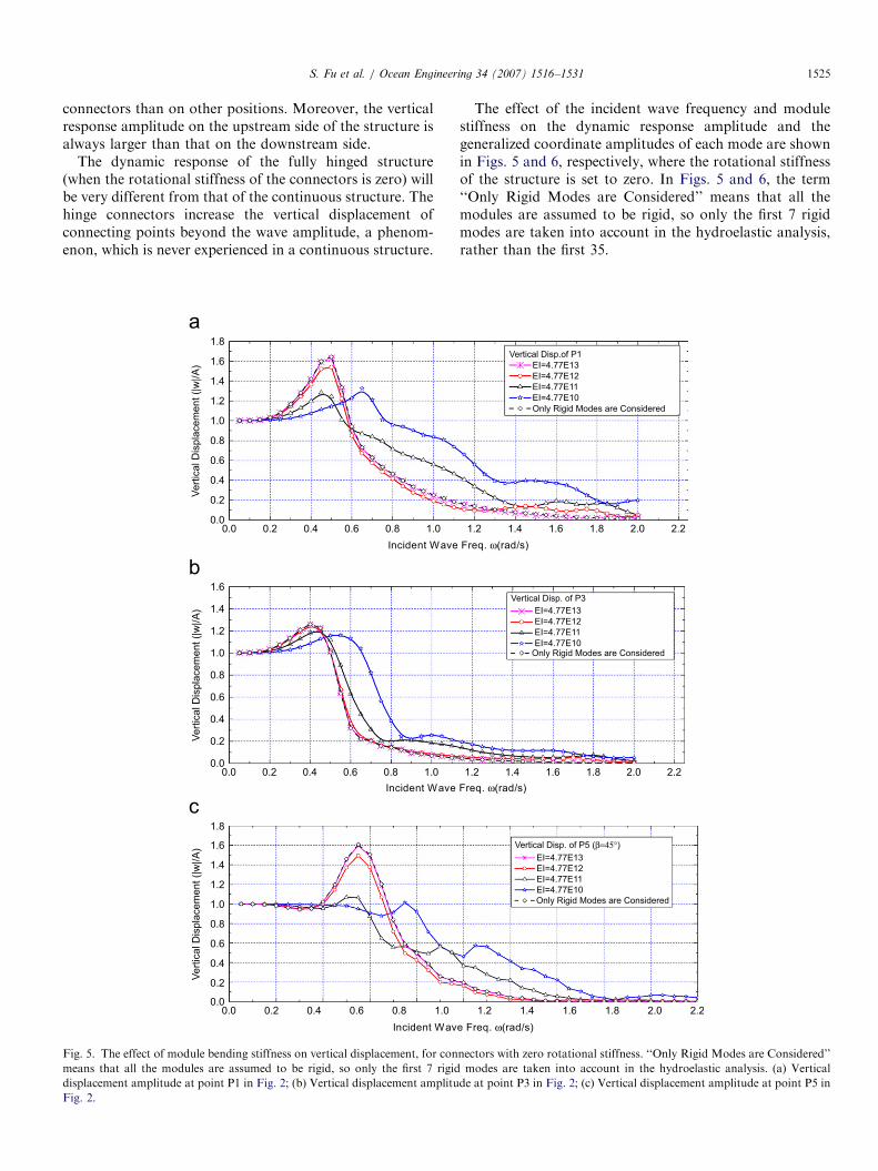
Fig. 5. The effect of module bending stiffness on vertical displacement, for con
means that all the modules are assumed to be rigid, so only the first 7 rigid
displacement amplitude at point P1 in Fig. 2; (b) Vertical displacement amplitu
Fig. 2.
The effect of the incident wave frequency and modulestiffness on the dynamic response amplitude and thegeneralized coordinate amplitudes of each mode are shownin Figs. 5 and 6, respectively, where the rotational stiffnessof the structure is set to zero. In Figs. 5 and 6, the term‘‘Only Rigid Modes are Considered’’ means that all themodules are assumed to be rigid, so only the first 7 rigidmodes are taken into account in the hydroelastic analysis,rather than the first 35.
Vertical Disp.of P1
EI=4.77E13
EI=4.77E12
EI=4.77E11
EI=4.77E10
Only Rigid Modes are Considered
1.2 1.4 1.6 1.8 2.0 2.2
Freq. ω(rad/s)
1.2 1.4 1.6 1.8 2.0 2.2
Freq. ω(rad/s)
1.2 1.4 1.6 1.8 2.0 2.2
e Freq. ω(rad/s)
Vertical Disp. of P3
Only Rigid Modes are Considered
Vertical Disp. of P5 (β=45°)EI=4.77E13
EI=4.77E12
EI=4.77E11
EI=4.77E10
Only Rigid Modes are Considered
EI=4.77E13
EI=4.77E12
EI=4.77E11
EI=4.77E10
nectors with zero rotational stiffness. ‘‘Only Rigid Modes are Considered’’
modes are taken into account in the hydroelastic analysis. (a) Vertical
de at point P3 in Fig. 2; (c) Vertical displacement amplitude at point P5 in
ARTICLE IN PRESSS. Fu et al. / Ocean Engineering 34 (2007) 1516–15311526
As can be seen from Figs. 5 and 6, the dynamic responseamplitude of points P1 and P3 is greatly affected by thebending stiffness of the module. The vertical amplitude hasits maximum value when the modules are assumed to berigid and only the first 7 rigid modes are included. In thedomain of relatively low-incident wave frequencies, in-
0.00.0 0.2 0.4 0.6 0.8 1
0.2
0.4
0.6
0.8
1.0
1.2
a
b
c
|P3|/A
|P7|/A
|P8|/A
Incident Wave
0.0 0.2 0.4 0.6 0.8 1
Incident Wave
0.0 0.2 0.4 0.6 0.8 1
Incident Wave
0.0
0.2
0.4
0.6
0.8
1.0
1.2
1.4
1.6
0.0
0.2
0.4
0.6
0.8
1.0
1.2
1.4
1.6
1.8
2.0
2.2
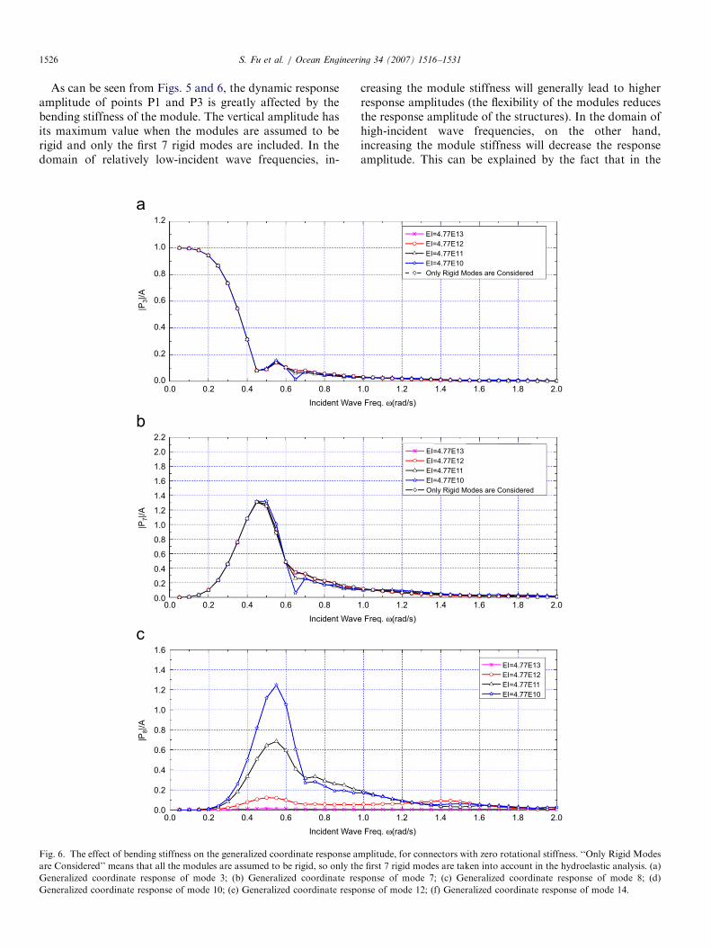
Fig. 6. The effect of bending stiffness on the generalized coordinate response a
are Considered’’ means that all the modules are assumed to be rigid, so only th
Generalized coordinate response of mode 3; (b) Generalized coordinate res
Generalized coordinate response of mode 10; (e) Generalized coordinate respo
creasing the module stiffness will generally lead to higherresponse amplitudes (the flexibility of the modules reducesthe response amplitude of the structures). In the domain ofhigh-incident wave frequencies, on the other hand,increasing the module stiffness will decrease the responseamplitude. This can be explained by the fact that in the
.0 1.2 1.4 1.6 1.8 2.0
EI=4.77E13
EI=4.77E12
EI=4.77E11
EI=4.77E10
Only Rigid Modes are Considered
Freq. ω(rad/s)
.0 1.2 1.4 1.6 1.8 2.0
Freq. ω(rad/s)
.0 1.2 1.4 1.6 1.8 2.0
Freq. ω(rad/s)
EI=4.77E13
EI=4.77E12
EI=4.77E11
EI=4.77E10
Only Rigid Modes are Considered
EI=4.77E13
EI=4.77E12
EI=4.77E11
EI=4.77E10
mplitude, for connectors with zero rotational stiffness. ‘‘Only Rigid Modes
e first 7 rigid modes are taken into account in the hydroelastic analysis. (a)
ponse of mode 7; (c) Generalized coordinate response of mode 8; (d)
nse of mode 12; (f) Generalized coordinate response of mode 14.
ARTICLE IN PRESS
0.0 0.2 0.4 0.6 0.8 1.0 1.2 1.4 1.6 1.8 2.0
EI=4.77E13
EI=4.77E12
EI=4.77E11
EI=4.77E10
EI=4.77E10
EI=4.77E13
EI=4.77E12
EI=4.77E11
EI=4.77E10
d
e
f
1.4
1.2
|P1
0|A
1.0
0.8
0.6
0.4
0.2
0.0
Incident Wave Freq. ω(rad/s)
0.0 0.2 0.4 0.6 0.8 1.0 1.2 1.4 1.6 1.8 2.0
Incident Wave Freq. ω(rad/s)
0.0 0.2 0.4 0.6 0.8 1.0 1.2 1.4 1.6 1.8 2.0
Incident Wave Freq. ω(rad/s)
|P1
2|/A
0.8
0.6
0.4
0.2
0.0
|P14|/A
0.5
0.4
0.3
0.2
0.1
0.0
EI=4.77E13
EI=4.77E12
EI=4.77E11
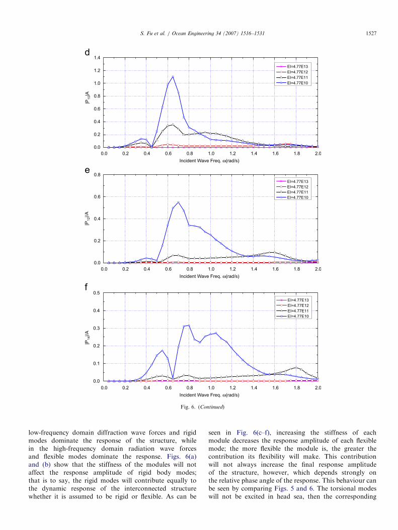
Fig. 6. (Continued)
S. Fu et al. / Ocean Engineering 34 (2007) 1516–1531 1527
low-frequency domain diffraction wave forces and rigidmodes dominate the response of the structure, whilein the high-frequency domain radiation wave forcesand flexible modes dominate the response. Figs. 6(a)and (b) show that the stiffness of the modules will notaffect the response amplitude of rigid body modes;that is to say, the rigid modes will contribute equally tothe dynamic response of the interconnected structurewhether it is assumed to be rigid or flexible. As can be
seen in Fig. 6(c–f), increasing the stiffness of eachmodule decreases the response amplitude of each flexiblemode; the more flexible the module is, the greater thecontribution its flexibility will make. This contributionwill not always increase the final response amplitudeof the structure, however, which depends strongly onthe relative phase angle of the response. This behaviour canbe seen by comparing Figs. 5 and 6. The torsional modeswill not be excited in head sea, then the corresponding
ARTICLE IN PRESS
0.0 0.2 0.4 0.6 0.8 1.0 1.2 1.4 1.6 1.8 2.0 2.20.0
0.2
0.4
0.6
0.8
1.0
1.2
1.4
1.6
1.8Vertical Disp. of P1
7 modes
8 modes
10 modes
14 modes
35 modes
Incident Wave Freq. ω(rad/s)
Ve
rtic
al D
isp
lace
me
nt
(|w
|/A
)
0.0 0.2 0.4 0.6 0.8 1.0 1.2 1.4 1.6 1.8 2.0 2.20.0
0.2
0.4
0.6
0.8
1.0
1.2
1.4
1.6
Incident Wave Freq. ω(rad/s)
Ve
rtic
al D
isp
lace
me
nt
(|w
|/A
)
Vertical Disp. of P3
7 modes
8 modes
10 modes
14 modes
35 modes
a
b
Fig. 8. The effect of the number of modes used in calculationon vertical displacement, for connectors with zero rotational stiffness. (a) Vertical
displacement amplitude at point P1 in Fig. 2, (b) Vertical displacement amplitude at point P3 in Fig. 2.
0.0 0.2 0.4 0.6 0.8 1.0 1.2 1.4 1.6 1.8 2.0
0.0
0.1
0.2
0.3
0.4
0.5
|P|/A
Incident Wave Freq. ω(rad/s)
β=45° Mode 9
Mode 11
Mode 13
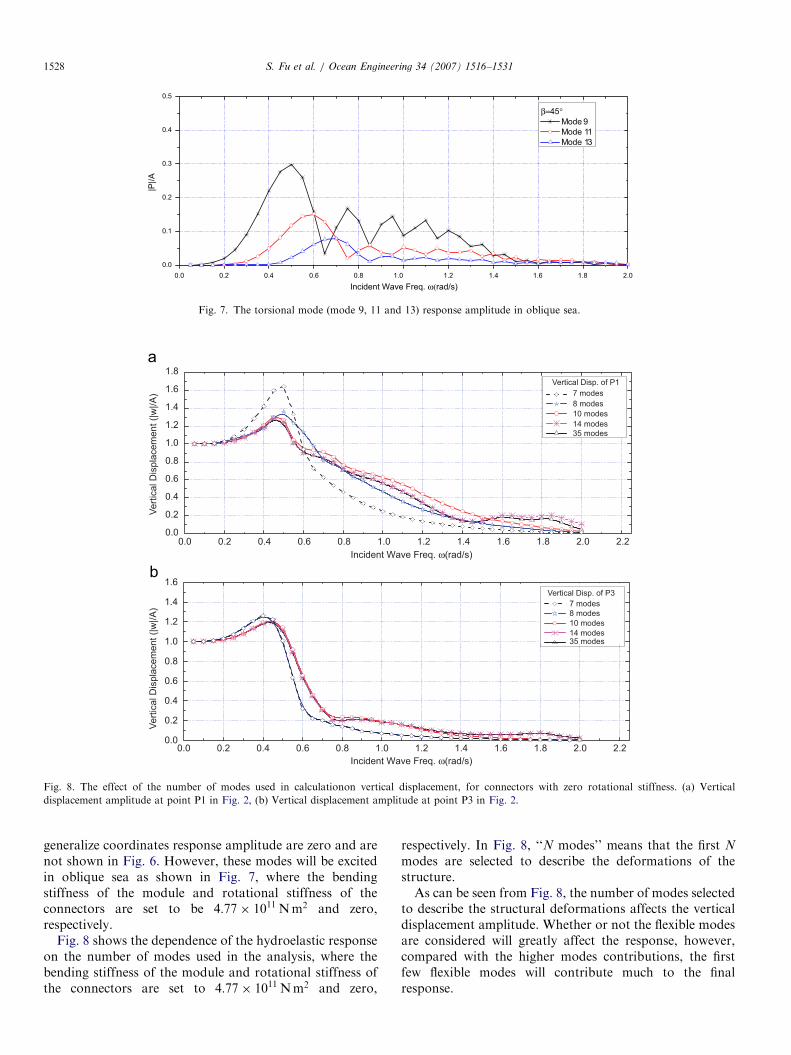
Fig. 7. The torsional mode (mode 9, 11 and 13) response amplitude in oblique sea.
S. Fu et al. / Ocean Engineering 34 (2007) 1516–15311528
generalize coordinates response amplitude are zero and arenot shown in Fig. 6. However, these modes will be excitedin oblique sea as shown in Fig. 7, where the bendingstiffness of the module and rotational stiffness of theconnectors are set to be 4:77� 1011 Nm2 and zero,respectively.
Fig. 8 shows the dependence of the hydroelastic responseon the number of modes used in the analysis, where thebending stiffness of the module and rotational stiffness ofthe connectors are set to 4:77� 1011 Nm2 and zero,
respectively. In Fig. 8, ‘‘N modes’’ means that the first N
modes are selected to describe the deformations of thestructure.As can be seen from Fig. 8, the number of modes selected
to describe the structural deformations affects the verticaldisplacement amplitude. Whether or not the flexible modesare considered will greatly affect the response, however,compared with the higher modes contributions, the firstfew flexible modes will contribute much to the finalresponse.
ARTICLE IN PRESS
0.0 0.2 0.4 0.6 0.8 1.0 1.2 1.4 1.6 1.8 2.00
50
100
150
200
250
Incident Wave Freq. ω(rad/s)
Cross Section at P2
Cross Section at P4
Be
nd
ing
Mo
me
nt
Mx (
MN
.m)
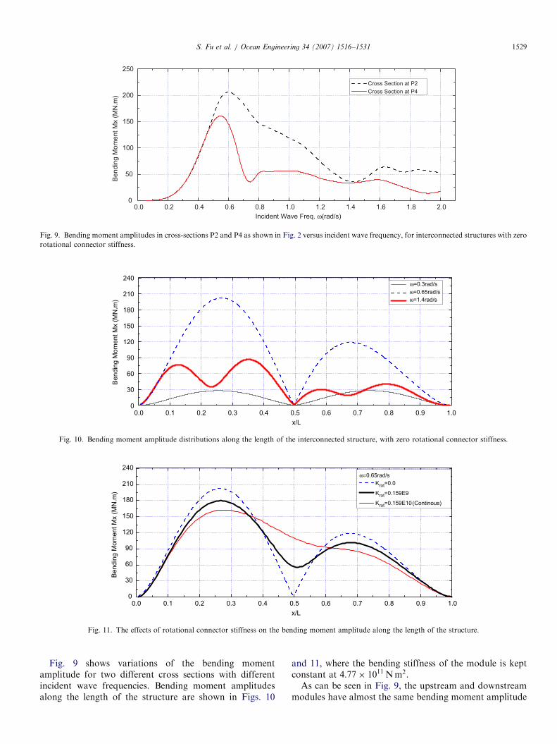
Fig. 9. Bending moment amplitudes in cross-sections P2 and P4 as shown in Fig. 2 versus incident wave frequency, for interconnected structures with zero
rotational connector stiffness.
0.0 0.1 0.2 0.3 0.4 0.5 0.6 0.7 0.8 0.9 1.00
30
60
90
120
150
180
210
240
Bendin
g M
om
ent M
x (
MN
.m)
x/L
ω=0.3rad/s
ω=0.65rad/s
ω=1.4rad/s
Fig. 10. Bending moment amplitude distributions along the length of the interconnected structure, with zero rotational connector stiffness.
0.0 0.1 0.2 0.3 0.4 0.5 0.6 0.7 0.8 0.9 1.00
30
60
90
120
150
180
210
240
Be
nd
ing
Mo
me
nt
Mx (
MN
.m)
x/L
ω=0.65rad/s
Krot=0.0
Krot=0.159E9
Krot=0.159E10(Continous)
Fig. 11. The effects of rotational connector stiffness on the bending moment amplitude along the length of the structure.
S. Fu et al. / Ocean Engineering 34 (2007) 1516–1531 1529
Fig. 9 shows variations of the bending momentamplitude for two different cross sections with differentincident wave frequencies. Bending moment amplitudesalong the length of the structure are shown in Figs. 10
and 11, where the bending stiffness of the module is keptconstant at 4:77� 1011 Nm2.As can be seen in Fig. 9, the upstream and downstream
modules have almost the same bending moment amplitude
ARTICLE IN PRESSS. Fu et al. / Ocean Engineering 34 (2007) 1516–15311530
for frequencies up to 0.45 rad/s. This means that rigid bodymotion dominates the interconnected structures, and thesefrequencies do not contribute to the bending moments ofthe structures. At higher frequencies the upstream modulewill always have a greater bending moment than thedownstream module. At a frequency of about 0.6 rad/s thebending moments of the upstream and downstreammodules reach their maximum values, which can beobserved by comparing Figs. 5, 6 and 9. Near thisfrequency, bending modes number 8, 10, 12 and 14, whichcontribute to the bending moment of the module, are allexcited by the incident wave.
As can be seen in Fig. 10, for low frequencies of theincident wave the upstream and downstream modules willhave almost the same bending moment amplitude. This isdue to the fact that the rigid body modes and diffractionwave forces dominate the motion and deflection of theinterconnected structure. As the incident wave frequencyincreases, the distribution of bending moments in the twomodules becomes more closely related to the flexible modesof each module. This phenomenon can also be observed bycomparing Figs. 5, 6 and 10.
Fig. 11 shows that the rotational connector stiffness alsoaffects the bending moment amplitude along the structure.As the rotational stiffness decreases from a very high value(representing a continuous structure) to zero, the bendingmoment in the middle of the structure decreases from itsmaximum value to zero. The bending moment within theupstream and downstream modules, on the other hand,will increase slightly.
5. Conclusions
This paper presents a hydroelastic theory of floatingstructures composed of flexible, interconnected modules. Anumerical example of a two-module structure is presented.The effects of connector and module stiffness on thehydroelastic response of the structure are studied, as well asthe characteristics of the bending moment distribution. Theresults show that the stiffness of the connectors and themodules is very important in determining the hydroelasticresponse of the structure.
References
Bathe, K.J., Wilson, E.L., 1976. Numerical Methods in Finite Element
Analysis. Prentice-Hall, Englewood Cliffs, NJ.
Bishop, R.E.D., Price, W.G., 1979. Hydroelasticity of Ships. Cambridge
University Press, UK.
Che, X.L., Wang, D.Y., Wang, M.L., Xu, Y.F., 1992. Two-dimensional
hydroelastic analysis of very large floating structures. Marine
Technology 29 (1), 13–24.
Che, X.L., Riggs, H.R., Ertekin, R.C., 1994. Composite 2D/3D
hydroelastic-analysis method for floating structures. Journal of
Engineering Mechanics 120 (7), 1499–1520.
Chen, X.J., Wu, Y.S., Cui, W.C., Tang, X.F., 2003a. Nonlinear
hydroelastic analysis of a moored floating body. Ocean Engineering
30 (8), 965–1003.
Chen, X.J., Jensen, J.J., Cui, W.C., Fu, S.X., 2003b. Hydroelasticity of a
floating plate in multidirectional waves. Ocean Engineering 30 (15),
1997–2017.
Cui, W.C., Yang, J.M., Wu, Y.S., Liu, Y.Z., 2007. Theory of
Hydroelasticity and its Application to Very Large Floating Structures.
Shanghai Jiao Tong University Press, to be published.
Eatock Taylor, R., 2003. Wet or Dry Modes in Linear Hydroelaticity—
Why Modes? Hydroelasticity in Marine Technology, Oxford, UK, pp.
239–250.
Eatock Taylor, R., Ohkusu, M., 2000. Green functions for hydroelastic
analysis of vibrating free-free beams and plates. Applied Ocean
Research 22, 295–314.
Ertekin, R.C., Kim, J.W., 1999. Hydroelastic response of floating mat-
type structure in oblique, shallow-water waves. Journal of Ship
Research 43 (4), 241–254.
Hamamoto, T., 1998. 3D hydroelastic analysis of module linked large
floating structures using quadratic BE-FE hybrid model, hydroelasti-
city in marine technology. In: Proceedings of the Second International
Conference on Hydroelasticity in Marine Technology, Fukuoka,
Japan, pp. 36–37.
Hermans, A.J., 1998. A boundary element method to describe the
excitation of waves in a very large floating flexible platform.
Hydroelasticity in Marine Technology, pp. 69–76.
Hibbit, Karlsson, Sorenson, 2004. ABAQUS Users’ Manual 6.5.
ABAQUS Inc.
Kashiwagi, M., 1998. A B-Spline Galerkin scheme for calculating the
hydroelastic response of a very large floating structure in waves.
Journal of Marine Science and Technology 1, 37–49.
Kim, D., Chen, L., Blaszkowski, Z., 1999. Linear frequency domain
hydroelastic analysis for McDermott’s mobile offshore base using
WAMIT. In: Proceedings of the Third International Workshop on
Very Large Floating Structures, VLFS’99, Honolulu, pp. 105–113.
Kim, J.W., Ertekin, R.C., 1998. An eigenfunction-expansion method for
predicting hydroelastic behavior of a shallow-draft VLFS. In:
Proceedings Second International Conference on Hydroelasticity in
Marine Technology (ICHMT98), Fukuoka, Japan, pp. 47–59.
Lee, C.H., Newman, J.N., 2000. An assessment of hydroelasticity for very
large hinged vessels. Journal of Fluid and Structures 14, 957–970.
Lee, C.H., Newman, J.N., 2004. WAMIT User’s Manual 6.2. WAMIT
Inc, MIT, MA, USA.
Newman J.N., 1997a. Wave effects on hinged bodies. Part I—body
motions, technical report /http://www.wamit.com/publications.
htmS.
Newman, J.N., 1997b. Wave effects on hinged bodies. Part II—hinge
loads, technical report /http://www.wamit.com/publications.htmS.
Newman, J.N., 1998a. Wave effects on hinged bodies. Part III—hinge
loads vs. number of modules, technical report /http://www.wamit.
com/publications.htmS.
Newman, J.N., 1998b. Wave effects on hinged bodies. Part IV—vertical
bending modes, technical report /http://www.wamit.com/publications.
htmS.Newman, J.N., 2005. Efficient hydrodynamic analysis of very large
floating structures. Marine Structures 16, 169–180.
Ohkusu, M., 1998. Hydroelastic behavior of floating artificial islands in
waves. Journal of the Society of Naval Architects of Japan 183, 239–248.
Riggs, H.R., Ertekin, R.C., 1993. Approximate methods for dynamic
response of multi-module floating structures. Marine Structures 6,
117–141.
Riggs, H.R., Ertekin, R.C., Mills, T.R.J., 1999. Impact of stiffness on the
response of a multimodule mobile offshore base. International Journal
of Offshore and Polar Engineering 9 (2), 126–133.
Riggs, H.R., Ertekin, R.C., Mills, T.R.J., 2000. A comparative study of
RMFC and FEA models for the wave-induced response of a MOB.
Marine Structures 13, 217–232.
Sahoo, T., Yip, T.L., Chwang, A.T., 2000. On the interaction of surface
wave with a semi-infinite elastic plate. In: Proceedings of the 10th
International Offshore and Polar Engineering Conference, Seattle,
USA, pp. 584–589.
ARTICLE IN PRESSS. Fu et al. / Ocean Engineering 34 (2007) 1516–1531 1531
Seto, H., Ochi, M. 1998. A hybrid element approach to hydroelastic
behavior of a very large floating structure in regular wave. Hydro-
elasticity in Marine Technology. In: Proceedings of the second
international conference on hydroelasticity in marine technology,
Fukuoka, Japan, pp.185–193.
Sim, I.H., Choi, H.S., 1998. An analysis of the hydroelastic behavior of
large floating structures in oblique waves. Hydroelasticity in
marine technology. In: Proceedings of the Second International
Conference on Hydroelasticity in Marine Technology, Fukuoka,
Japan, pp. 165–169.
Sun, H., Song, H., Cui, W.C., 2002. On the interaction of surface waves
with an elastic plate of finite length in head seas. China Ocean
Engineering 16 (1), 21–32.
Taghipour, R., Fu, S.X., Moan, T., 2006. Validated two and
three dimensional linear hydroelastic analysis using standard soft-
ware. In: Proceedings of the 16th International Offshore and
Polar Engineering Conference, San Francisco, California, USA, pp.
101–107.
Wang, D.Y., Riggs, H.R., Ertekin, R.C., 1991. Three-dimensional
hydroelastic response of a very large floating structure. International
Journal of Offshore and Polar Engineering 1 (4), 307–316.
Wu, C., Watanabe, E., Utsunomiya, T., 1995. An eigenfunction expansion
matching method for analysis wave-induced response of a large
floating plate. Applied Ocean Research 17, 301–310.
Wu, M.K., Moan, T., 1996. Linear and nonlinear hydroelastic analysis of
high-speed vessels. Journal of Ship Research 40 (2), 149–163.
Wu, Y.S., 1984. Hydroelasticity of floating bodies, Ph.D. Thesis, Brunel
University, UK.
Wu, Y.S., Wang, D.Y., Riggs, H.R., Ertekin, R.C., 1993. Composite
singularity distribution method with application to hydroelasticity.
Marine Structures 6, 143–163.
Xia, J.Z., Wang, Z.H., Jensen, J.J., 1998. Non-linear wave loads and ship
responses by a time-domain strip theory. Marine Structure 11 (3), 101–123.
Yago, K., Endo, H., 1996. On the hydroelastic response of boxshaped
floating structure with shallow draft. Journal of the Society of Naval
Architects of Japan 180, 341–352.