hydrodynamic modelling study of a … · design of the unit, computational fluid dynamics has been...
TRANSCRIPT

Eleventh International Conference on CFD in the Minerals and Process Industries
CSIRO, Melbourne, Australia
7-9 December 2015
Copyright © 2015 CSIRO Australia 1
HYDRODYNAMIC MODELLING STUDY OF A ROTATING
LIQUID SHEET CONTACTOR
Christopher B. SOLNORDAL1* Andrew ALLPORT2 and Leigh T. WARDHAUGH3
1 CSIRO Mineral Resources, Clayton, Victoria 3169, AUSTRALIA
2 CSIRO Services, Newcastle, 2300, AUSTRALIA
3 CSIRO Energy, Newcastle, 2300, AUSTRALIA *Corresponding author, E-mail address: [email protected]
ABSTRACT
The Rotating Liquid Sheet contactor is a recently
developed gas-liquid contactor capable of providing high
interphase contact in combination with a low associated
pressure drop of flowing gas. The device consists of a
cylindrical flow passage and a central rotating tube with
helical slots in its walls. Liquid passes into the central tube
and out through the slots, forming continuous sheets of
liquid in the shape of helices or compressor blades,
depending on the slot design. Gas passes through the
annular gap between the cylinder and central tube. By
rotating the central tube, the liquid sheets provide high
surface area for interphase contact while simultaneously
pumping gas through the device. In order to optimise
design of the unit, computational fluid dynamics has been
used at many stages of the development process. This
paper describes attempts to model the gas flow through the
unit, the liquid flow through the central tube, and the
dynamics of the liquid sheet. It was found that the unit is
capable of pumping gas through it using the helical liquid
sheet. Also profiled struts along the slots were required to
produce a uniform horizontal flow of liquid through them.
An extremely fine mesh was required to allow modelling
of the liquid sheet. The stability of the predicted liquid
sheet was found to be highly sensitive to the specified
surface tension. However, by using a surface tension value
lower than the standard value for water, a uniform sheet
with parabolic profile was predicted, as was observed
experimentally.
INTRODUCTION
Traditional packed column gas-liquid contactors are a
mature technology that offer little in the way of potential
process improvements. Increasing gas flow causes liquid
entrainment, while gravity-fed liquid flow rate is limited
by the liquid viscosity. A novel type of gas-liquid
contactor is the Rotating Liquid Sheet (RLS) contactor,
recently developed and patented by the authors
(Wardhaugh et al. 2012, Wardhaugh et al. 2015). The
RLS contactor creates a sheet of liquid within a cylindrical
flow passage. The sheet surface is that of a number of
continuous helices or else short blade-like surfaces, so that
when rotated the liquid surface pumps gas through the
device, in a manner similar to a screw conveyor. The
system is shown schematically in Figure 1a for a single
continuous helical liquid sheet. Figure 1b shows a
photograph of an air-water laboratory scale model of the
contactor where the stability of the liquid sheet is visible
for the conditions studied. Features of the photograph are
identified in Figure 1c. Compared to a packed column, the
RLS contactor allows increased gas throughput with
negligible liquid entrainment in the gas stream, and the
use of higher viscosity liquids. Furthermore, the pumping
action of the liquid sheet decreases the pressure loss for
gas passing through the system.
Figure 1: (a) Schematic diagram of RLS contactor; (b)
photograph of liquid film; (c) diagram explaining features
in photograph.
In order to understand and optimise the fluid
mechanics of the RLS contactor, CFD modelling has been
used extensively. However, the complexity of the system
meant that it was difficult to model the entire unit at once,
so instead three separate models were used to investigate
different aspects of the contactor design. The feasibility of
pumping gas through the unit was initially investigated

Copyright © 2015 CSIRO Australia 2
using a single phase model where the liquid sheet was
modelled as a solid helical surface. The flow through the
central tube and helical slot was modelled as a single
liquid phase to investigate slot design. Finally, the
dynamics of the liquid sheet itself was explored using a
two phase air-water model extending from the helical slot
to the outer wall of the device. Each of the three models
was developed using Eulerian analyses within ANSYS
CFX (ANSYS 2013), and are presented in turn.
CFD MODEL 1 – SOLID HELICAL SURFACE
The purpose of the solid helical surface model was to
investigate the gas flow dynamics through a rotating helix,
and to determine if such a helix could induce flow through
it purely by rotation.
Geometry, Mesh and Boundary Conditions
The solid helical surface model geometry is
represented by the schematic diagram of the RLS
contactor in Figure 1a. The flow domain had a central tube
outer diameter of 25.4 mm and an external wall inner
diameter of 150 mm (Figure 1c) and extended 2 m
upstream and 2 m downstream of the single solid helical
surface. Such distances were required to ensure
boundaries did not interfere with the action of the rotating
solid surface on the gas flow. The solid helical surface
represented the liquid sheet, and turned six times around
the central tube at a pitch of 23.2 mm, with uniform
thickness of 0.7 mm.
The fluid for this model was air at room temperature
and pressure, with standard properties. Pressure
boundaries (P = 0 Pa g) were specified at the inlet and
outlet of the domain, while the inner and outer walls as
well were modelled as no-slip walls. It was not clear
whether a no-slip or free-slip boundary would best
represent the fluid interaction at the solid helical surface,
since in reality the helix is a flowing liquid. A no-slip
condition was used in the first instance, while comparison
to free-slip or other conditions at this surface was left for
future work. A 1 mm gap was left between the external
wall and the solid helical surface, and a hexahedral mesh
was imposed on the flow domain in such a way that the
central tube and solid helical surface could rotate within
the thin outer shell that represented the external wall. The
mesh had a total of approximately 1.2 million elements,
which were concentrated around and immediately
upstream and downstream of the helical blade.
Although many runs were performed, varying both
vane pitch and rotation rate, here the results are presented
for pitch of 23.2 mm and rotation speed of 600 RPM.
Transient simulations were performed using a time step
equal to 0.008333 s, which corresponded to a centrebody
rotation of 30. A total of 120 time steps were calculated,
to simulate 10 full revolutions of the centrebody. During
the simulation the longitudinal flow field remained steady,
suggesting that the 10 revolutions was adequate to capture
the detail of the flow.
Results
The predicted instantaneous velocity profile in a
vertical plane centred on the geometry axis is shown in
Figure 2. Figure 2a shows the elevation view between two
successive surfaces approximately half way up the helix.
The distribution did not vary greatly from the lower to the
upper sections of the 6-turn surface, and a reasonably
steady upward velocity is predicted. Higher velocities are
shown at larger radii, but this is primarily due to the drag
between the air and the solid vane causing increased
tangential velocity. This behaviour is shown in Figure 2b
(air velocity vector profile in plan view – distribution
profile shown by white line), where velocity increases
slightly with radial position. The black line in Figure 2b
indicates the velocity profile of the solid vane surface, and
the air velocity is only approximately 20-30% of this
value. Thus the amount of swirling motion imparted to the
air is small compared to the actual rotational velocity of
the vane. In the real system the drag between the liquid
sheet and the gas is likely even smaller since the “no slip”
condition imposed here may not apply. Figure 2a also
shows the existence of a recirculation trailing the outer
edge of the solid vane, near the outer wall of the device.
Such a flow is likely to occur on the actual device since
there would be upward flow of gas in the main bulk of the
flow passage but downward flow of liquid at the outer
surface, thus forcing a recirculatory flow.
At the rotation rate of 600 RPM the bulk vertical
velocity is predicted to be 0.177 m s-1, which is 76% of the
value expected if the vane were to transport the fluid as a
solid body.
Figure 2: Velocity vector plot for flow through rotating
solid helical surface model. Rotation speed = 600 RPM.
CFD MODEL 2 – CENTRAL TUBE
The purpose of the central tube model was to
determine a design that could produce a uniform
horizontal flow of fluid through the helical slot(s). This is
important because if the flow is uneven, then successive
layers of the helical film may fall onto those beneath,
decreasing the available interfacial surface area for mass
transfer and potentially reducing the pumping efficiency of
the device. Many different geometries were investigated,
and some typical ones are presented in this section (see
Figure 3).
Geometry, Mesh and Boundary Conditions
The flow through the central tube was modelled
primarily as a single phase, with the fluid being water at

Copyright © 2015 CSIRO Australia 3
room temperature (although some two-phase air-water
modelling did take place). A typical geometry is shown in
Figure 3a, where a single slot at angle of 45 to the tube
axis completes a single rotation around the tube wall. The
outer and inner diameters of the tube are labelled, and
equal to 25.4 mm and 22.2 mm respectively, producing a
wall thickness of 1.6 mm. The full geometry extends
vertically a total length of 250 mm, although the entrance
length is not shown in the Figure; fluid enters from above
and the bottom surface is solid so that all fluid is forced
through the helical slot. In this case the slot width is
1.2 mm. Images in Figure 3b-d show examples of
changing slot width and profile, changing wall thickness,
inclusion of a central rod and modifying its longitudinal
profile, the use of multiple helical slots, short rows of
multiple “blade”-like slots, helical structures on the central
rod, and horizontal ribs through the slot to act as flow
straighteners.
Inlet velocities were specified to provide a given
average outlet velocity through the slot that varied from
1 m s-1 to 5 m s-1. The effect of rotation was also
investigated (although results are not reported here). All
walls were treated as no-slip boundaries, while the inlet
was a simple Dirichlet boundary and the slot outlet had a
constant pressure boundary of 0 Pa g applied. Simulations
were performed under steady state conditions on a
tetrahedral mesh with wall inflation. Eight cells were used
across the slot, and all geometric features shown in the
figures were explicitly meshed. Each mesh had
approximately 3 million elements.
Results
Predicted flow patterns for four selected centrebody
geometries are presented in Figure 4. Figure 4a shows
streamlines coloured by speed of water. The standard
single slot geometry A demonstrates significant
recirculation of fluid, while use of a central rod in
geometry C leads to a more uniform vertical flow of fluid
and less recirculation, albeit at a higher velocity due to the
decreased cross-sectional area. The flow uniformity is
improved further using geometry F which has four helical
slots through a thicker wall, and a central rod. However,
geometry F also shows streamlines travelling at a
significant downward angle through the slots rather than
horizontally outwards. Geometry I attempts to alleviate
this flow feature by using three rows of four short slots,
each of which has guide vanes positioned to attempt to
create a more uniformly horizontal flow pattern at the slot
outlet. The geometry appears to achieve this to some
extent. In Figure 4b the velocity vector field at the slot
outlets are shown for each geometry, and the vectors are
coloured by the local vertical component of velocity. In all
cases there is a tendency for flow to exit the slots in a
downward direction (green-blue to blue vectors), and this
is most pronounced for Geometry F. Geometry I is
predicted to produce a more horizontal throw of fluid.
Despite the promising flow field predicted for geometry I,
experimental tests using such a geometry (created using
additive manufacturing) showed that this bladed geometry
produced many liquid sheet edges that tended to curl in
towards the centre of the sheet. Therefore, ongoing work
is now considering the use of continuous sheets.
Also of interest is for the centrebody to produce a
uniform flow along the length of the slot. To investigate
this behaviour the slots for geometries A-E (as well as
some others not shown) were divided into eight equal
segments, numbered 01 (at the top of the slot) to 08 (at the
bottom, see Figure 1c).
Figure 3: Different centrebody designs, labelled A-I.
The flow rate (expressed as a Reynolds number using slot
width as the length scale) is plotted as a function of outlet
location in Figure 5, and for all geometries studied the
Reynolds number generally increased with downstream
distance, although there was a slight tendency for the
maximum flow to occur at outlet 06 rather than outlet 08.
Geometries that used a greater wall thickness tended to
give a greater variation in Reynolds number along the
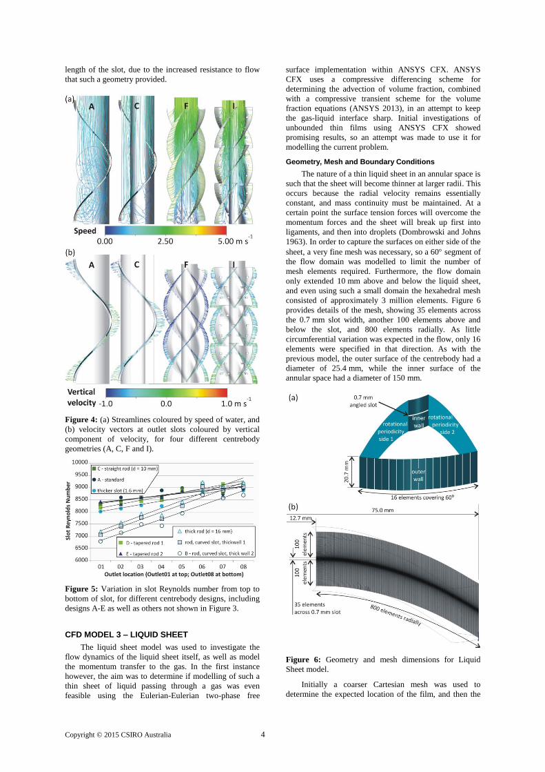
Copyright © 2015 CSIRO Australia 4
length of the slot, due to the increased resistance to flow
that such a geometry provided.
Figure 4: (a) Streamlines coloured by speed of water, and
(b) velocity vectors at outlet slots coloured by vertical
component of velocity, for four different centrebody
geometries (A, C, F and I).
Figure 5: Variation in slot Reynolds number from top to
bottom of slot, for different centrebody designs, including
designs A-E as well as others not shown in Figure 3.
CFD MODEL 3 – LIQUID SHEET
The liquid sheet model was used to investigate the
flow dynamics of the liquid sheet itself, as well as model
the momentum transfer to the gas. In the first instance
however, the aim was to determine if modelling of such a
thin sheet of liquid passing through a gas was even
feasible using the Eulerian-Eulerian two-phase free
surface implementation within ANSYS CFX. ANSYS
CFX uses a compressive differencing scheme for
determining the advection of volume fraction, combined
with a compressive transient scheme for the volume
fraction equations (ANSYS 2013), in an attempt to keep
the gas-liquid interface sharp. Initial investigations of
unbounded thin films using ANSYS CFX showed
promising results, so an attempt was made to use it for
modelling the current problem.
Geometry, Mesh and Boundary Conditions
The nature of a thin liquid sheet in an annular space is
such that the sheet will become thinner at larger radii. This
occurs because the radial velocity remains essentially
constant, and mass continuity must be maintained. At a
certain point the surface tension forces will overcome the
momentum forces and the sheet will break up first into
ligaments, and then into droplets (Dombrowski and Johns
1963). In order to capture the surfaces on either side of the
sheet, a very fine mesh was necessary, so a 60 segment of
the flow domain was modelled to limit the number of
mesh elements required. Furthermore, the flow domain
only extended 10 mm above and below the liquid sheet,
and even using such a small domain the hexahedral mesh
consisted of approximately 3 million elements. Figure 6
provides details of the mesh, showing 35 elements across
the 0.7 mm slot width, another 100 elements above and
below the slot, and 800 elements radially. As little
circumferential variation was expected in the flow, only 16
elements were specified in that direction. As with the
previous model, the outer surface of the centrebody had a
diameter of 25.4 mm, while the inner surface of the
annular space had a diameter of 150 mm.
Figure 6: Geometry and mesh dimensions for Liquid
Sheet model.
Initially a coarser Cartesian mesh was used to
determine the expected location of the film, and then the

Copyright © 2015 CSIRO Australia 5
fine curvilinear mesh in Figure 6 was created so that the
mesh elements could follow the same path as the film.
The film velocity at the slot was specified to be
1 m s-1 in the radial direction with zero vertical component
of velocity. The boundaries above and below the film were
specified as openings at constant atmospheric pressure,
while the outer and inner walls had a no-slip wall surface
condition. The side boundaries were assigned rotational
periodicity boundary conditions so that any fluid flowing
out of one boundary would flow back into the flow
domain at the other boundary. This feature was important
once rotational motion was added to the simulation. In
order to simulate rotation of the film, the flow domain
could be specified as rotating, and simulations were
performed at 0, 100, 200 and 300 RPM.
The liquid flow was assumed to be laminar, since the
slot Reynolds number was equal to 786. Standard values
of air and water density and viscosity were used in the
model. It was found that the results were strongly sensitive
to the air-water surface tension specified in the model, and
the most reliable way to produce a stable film solution (in
agreement with experimental observation) was to neglect
surface tension altogether. The issue of surface tension
sensitivity is addressed in the Discussion.
A transient solution to the equations of motion were
performed with a time step of 0.0005 s, leading to an RMS
Courant number of less than 1, indicating time resolution
was adequate for the current mesh. A constant time step
was used as convergence difficulties sometime occurred
when using a variable time step.
Results
The predicted film surface is shown in Figure 7a, as a
surface equal to liquid volume fraction of 0.05. The
surface is coloured by the local liquid velocity, which
starts at 1.0 m s-1 at the slot exit and increases slightly
towards the outer wall of the device, due to gravitational
acceleration. Figure 7b shows an elevation view of the
centreline of the film, in this case coloured by liquid
volume fraction. The path of the film curves smoothly
towards the outer wall of the device, following a parabolic
path. The thickness of the film – defined approximately by
the number of grid cells that are coloured red and
therefore have a liquid volume fraction equal to 1 –
reduces with radial distance until about half way to the
outer wall of the device. At this point the liquid has
diffused across several mesh cells so that no cell is
completely filled with liquid. Figure 7c-j shows detail of
the film at successive locations along the film, and by
position (g) the film is predicted to be smeared over
approximately 16 cells, with none of those cells containing
only water. At locations h-j a stratification of the film is
predicted, with layers of liquid 2-3 cells thick. In Figure 7j
the film is shown to hit the outer wall and the volume
fraction increases once more to a value of 1.
The numerical diffusion at the top and bottom
surfaces of the film is believed to be an artefact of the
technique used to define the air-water interface in ANSYS
CFX. The stratification shown in Figure 7h-j is also
expected to be a result of the numerical techniques, and
not a real phenomenon.
Figure 8 shows the film surface at increasing rates of
rotation. In order to better visualise the surface of the film,
the geometry is repeated six times around the central axis
of the device, so that it appears there are six short angled
slots around the central tube, each generating its own
liquid film. The film is coloured by the vertical position of
the surface to help visualise its shape. The image shows
how the leading edge trails the rotating centrebody by
increasing amounts with each increase in rotation.
However, the actual velocity of individual liquid elements
remains radial in direction, as indicated by the vector plot
at 300 RPM shown in plan view in Figure 8e. There is a
similar issue in prediction of the liquid film surface using
a rotating centrebody, in that the film initially is predicted
to become thinner with radial distance (like Figure 7c-j)
but ultimately spreads out over several mesh elements with
water volume fraction less than one.
Figure 7: Detail of predicted film surface at 0 RPM. (a)
Isometric view; (b) elevation view; (c-j) successive detail
of elevation view, showing mesh structure.
A more realistic boundary condition might be to add
the circumferential component of rotation at the slot to the
liquid velocity. This would presumably predict a straighter
leading edge to the film.
The film becomes discontinuous near the outer wall at
300 RPM (Figure 8d) because the rotationally periodic
boundaries do not overlap perfectly, but instead one side
is higher than the other (see Figure 9a). For the case of
300 RPM rotation, the film exits one periodic boundary

Copyright © 2015 CSIRO Australia 6
quite high up and then cannot re-enter the opposite
boundary as there is no region of overlap between the two
at that location (see location of film on the periodic
boundary, shown as a thick white line in Figure 9b for
100 RPM rotation, and Figure 9c for 300 RPM rotation).
Figure 8: Film surface at (a) 0 RPM; (b) 100 RPM; (c)
200 RPM, and (d) 300 RPM. (e) Plan view of water
velocity vectors at 300 RPM.
DISCUSSION – SURFACE TENSION ON THIN
FILMS
On addition of surface tension values to the Liquid
Sheet model, the model predicts the film to become
unstable. Figure 10 shows instantaneous values of the
liquid sheet using increasingly large values of surface
tension up to the value of 0.072 N m-1 typically quoted for
air-water systems. At values of 0.001 N m-1 the film is
generally stable, but has occasional regions of break-up
(Figure 10b). Using larger values shows significant
breakup of the sheet, in contradiction to experimental
observation.
Figure 9: (a) wireframe view of successive 60 segments,
showing that periodic boundary interfaces do not overlap
perfectly; (b) White line shows film at 100 RPM stays
within the overlapping region; (c) White lines show film at
300 RPM strays outside the overlapping region of the
periodic boundaries.
Further investigations have been performed to try and
understand the cause of this prediction. The system was
simplified to one of a downward facing film falling
vertically under gravity, and by increasing the resolution
of the mesh in all three dimensions it was possible to
produce a uniform film with surface tension equal to
0.072 N m-1. However, as soon as the gravity vector is
mis-aligned with the direction of fluid entry, the film is
predicted to become unstable.
Upon reading the source literature of the ANSYS
CFX surface tension model (Brackbill et al. 1992) it was
thought local radius of curvature effects might be causing
difficulties, and it was for this reason that the mesh in
Figure 6b was aligned with the direction of film flow.
However, even with aligned mesh structure and using a
10 sector (c.f. 60) with increased resolution it was not
possible to predict a stable film. Direct numerical
simulation of a round jet by Shinjo (Shinjo and Umemura
2010) has demonstrated that analyses of thin liquid
structures such as ligaments and droplets using Brackbill’s
surface tension model is possible, however they required
up to 6 billion elements for their analysis, and claimed that
at least 8 cells across any structure was required to
produce realistic results. Use of ANSYS FLUENT with
volume-of-fluid techniques to determine free surface
location, and mesh adaption to maintain resolution of the
mesh where required, is being investigated by the authors.

Copyright © 2015 CSIRO Australia 7
Figure 10: Early simulations of liquid sheet model with
increasing values of surface tension.
CONCLUSIONS AND FUTURE WORK
The use of CFD to analyse and understand the operation
of a novel gas-liquid contactor has been undertaken. Three
separate models of the system were developed in order to
break down a complex system into more manageable
problems, and the results have generally been in keeping
with experimental observation. Ongoing difficulties in
predicting surface tension effects on thin films are still to
be resolved. Initial work has begun on investigating the
mass transfer between gas and liquid in the system, and
using ANSYS FLUENT to improve simulation of the film.
REFERENCES
ANSYS (2013). ANSYS-CFX15.0 User Manual.
Canonsburg, PA, USA, ANSYS Inc.
BRACKBILL, J. U., KOTHE, D. B. and ZEMACH,
C. (1992). "A Continuum Method for Modeling Surface-
Tension." Journal of Computational Physics 100(2): 335-
354.
DOMBROWSKI, N. and JOHNS, W. R. (1963).
"The Aerodynamic Instability and Disintegration of
Viscous Liquid Sheets." Chemical Engineering Science
18(3): 203-&.
SHINJO, J. and UMEMURA, A. (2010). "Simulation
of liquid jet primary breakup: Dynamics of ligament and
droplet formation." International Journal of Multiphase
Flow 36(7): 513-532.
WARDHAUGH, L. T., ALLPORT, A.,
SOLNORDAL, C. B. and FERON, P. H. M. (2015). "A
novel type of gas-liquid contactor for post-combustion
capture cost reduction." Greenhouse Gases-Science and
Technology 5(2): 198-209.
WARDHAUGH, L. T., CHASE, D. R., GARLAND,
E. A. and SOLNORDAL, C. B. Gas and liquid phase
contactor used in oil and gas industries, has gas inlet that
directs gas through gas liquid contacting space into
contact with each side of liquid sheets projected from
outlets in housing.,WO2012103596-A1 (2012).