hydrodynamic and acoustic performance analysis of marine

Mathematical

and Computational

Applications

Article

Hydrodynamic and Acoustic Performance Analysis ofMarine Propellers by Combination of Panel Methodand FW-H Equations

Abouzar Ebrahimi 1 , Mohammad Saeed Seif 1,* and Ali Nouri-Borujerdi 2

1 Center of Excellence in Hydrodynamic and Dynamic of Marine Vehicles, Sharif University of Technology,Tehran, Iran

2 Mechanical Engineering Department, Sharif University of Technology, Tehran, Iran* Correspondence: [email protected]

Received: 13 August 2019; Accepted: 5 September 2019; Published: 9 September 2019

Abstract: The noise emitted by ships is one of the most important noises in the ocean, and the propellernoise is one of the major components of the ship noise. Measuring the propeller noise in a laboratory,despite the high accuracy and good reliability, has high costs and is very time-consuming. For thisreason, the calculation of propeller noise using numerical methods has been considered in recent years.In this study, the noise of a propeller in non-cavitating conditions is calculated by the combination ofthe panel method (boundary element method) and solving the Ffowcs Williams-Hawkings (FW-H)equations. In this study, a panel method code is developed, and the results are validated by theexperimental results of the model tests carried out in the cavitation tunnel of the Sharif University ofTechnology. Software for numerical calculation of propeller noise, based on FW-H equations, is alsodeveloped and the results are validated by experimental results. This study shows that the results ofthe panel method code have good agreement with experimental results, and that the maximum errorof this code for the thrust and torque coefficients is 4% and 7%, respectively. The results of the FW-Hnoise code are also in good agreement with the experimental data.

Keywords: panel method; marine propeller; noise; FW-H equations; experimental test

1. Introduction

In recent years, the use of numerical methods has become very common in modeling the flowaround marine propellers. Although the experimental methods have a higher accuracy and reliabilitythan numerical methods, the higher costs and the need for special equipment has caused numericalmethods to be preferred.

The boundary element method (BEM) is one of the methods used to solve the governing equationsof fluid mechanics, acoustics, electromagnetics, etc. In this method, using mathematical theorems,the equations from the interior of the solution domain are transferred to the boundaries of the domain.Therefore, compared to other numerical methods such as finite element or finite volume method whichinterior of domain should be considered, BEM exhibits less solution time and computation cost andtherefore it is preferred to other methods.

The panel method is one of boundary element methods. In this method, the surface of the bodyis divided into small panels and a combination of source and doublets is distributed to each panel.After calculating the strength of sources and doublets, velocity and pressure distribution on surfacepanels can be obtained. For lifting bodies, a wake surface should be assumed at the trailing edge ofbody, and the effect of panels of this surface on body panels should be considered.

In recent decades, the panel method has been widely used to solve the flow around the bodies,especially marine propellers. A literature review shows that a lot of research has been done on the

Math. Comput. Appl. 2019, 24, 81; doi:10.3390/mca24030081 www.mdpi.com/journal/mca

http://www.mdpi.com/journal/mca

http://www.mdpi.com

https://orcid.org/0000-0003-2576-363X

http://www.mdpi.com/2297-8747/24/3/81?type=check_update&version=1

http://dx.doi.org/10.3390/mca24030081

http://www.mdpi.com/journal/mca

Math. Comput. Appl. 2019, 24, 81 2 of 18

use of the panel method for the hydrodynamic analysis of objects. For instance, Hess and Smith [1],in 1962, invented the panel method for analyzing the motion of three dimensional bodies in fluid.The formulation of these researchers was presented for the arbitrary three dimensional bodies andcould not be used for lifting bodies. In 1972, Hess [2] developed this method for lifting bodies andcalculated the pressure distribution around an aircraft model and lift force. The panel method wasfirst used in 1985 by Hess and Valarezo [3] to model the flow around the ship propeller. In this study,they obtained the pressure distribution around a propeller using quadrilateral panels and calculatedthe thrust and torque coefficients. In 2010, Baltazar et al. [4] modeled cavitation around a propellerusing the panel method. The results of this study show that the panel method can model cavitation onpropeller blades with good accuracy. Also, several papers have been published between the years 1985to 2010, but most have done similar work.

In 2010, Gaggero et al. [5] modeled the flow around the propeller using the panel method andcomputational fluid dynamics. The results of the panel method show that this method has a good andacceptable accuracy compared to the CFD method.

According to the importance of propeller noise, various methods have been proposed to reduce it.Methods used to reduce the noise of marine propellers can be divided into two main methods, namely:

- Using equipment- Modification of the geometry

Each of these methods is fully described in a review paper published by Ebrahimi et al. [6].In recent years, calculating the noise of marine propellers using numerical methods has also beendeveloped by researchers. For numerical calculation of noise, a numerical method such as panelmethod is required to obtain flow quantities and then these quantities are used as input for calculationof noise for a receiver at the desired location. Seol and Park [7] carried out several experiments on apropeller model in MOERI cavitation tunnel and measured the noise of propeller in cavitating andnon-cavitating condition. Also, they used combination of time domain acoustic analogy and panelmethod for the numerical investigation of the propeller noise.

In another study by Kellett et al. [8] in 2013, the noise generated by the propeller of a LNG carriership was measured numerically and experimentally. Bagheri et al. [9] conducted a research on a threebladed propeller of the Gawn series and used the ANSYS Fluent commercial software for calculation ofthe propeller noise. Testa et al. [10] calculated the noise of E779A propeller model by using the FW-Hequations in presence of unsteady sheet cavitation. They also used potential-based panel method formodelling flow around propeller. Gorji et al. [11] performed a research on calculation of noise of amarine propeller using a RANS solver in the low frequencies band.

Bagheri et al. [12] carried out some numerical and experimental tests on the noise of marinepropellers and the effects of cavitation on the sound pressure level of propeller. They used viscousflow with FW-H solver for noise calculation.

In present research, a boundary element method is used for hydrodynamic analysis of marinepropellers. Also, the FW-H equations are used for acoustic performance analysis of these propellers.For this purpose, two codes have been developed by authors and their results validated usingexperimental tests carried out in cavitation tunnel of Sharif University of Technology. The mostsignificant novelty of our paper is that we used experimental noise measurements to validate theresults of the FW-H equations code.

2. Formulation of the Panel Method

For development of the panel method formulation for marine propeller, the flow aroundpropeller in computational domain of Ω is assumed to be irrotational, incompressible and inviscid.By these assumptions, the flow governing equations (Navier-Stokes equation) are simplified into


the three-dimensional Laplace equation where is ∇2φ. By using Green’s second identity, the generalsolution of this equation is as follows [13]:∫

Ω

(φ1∇

2φ2 −φ2∇2φ1

)dV =

∫S

(φ1∇φ2 −φ2∇φ1) ·→ndS (1)

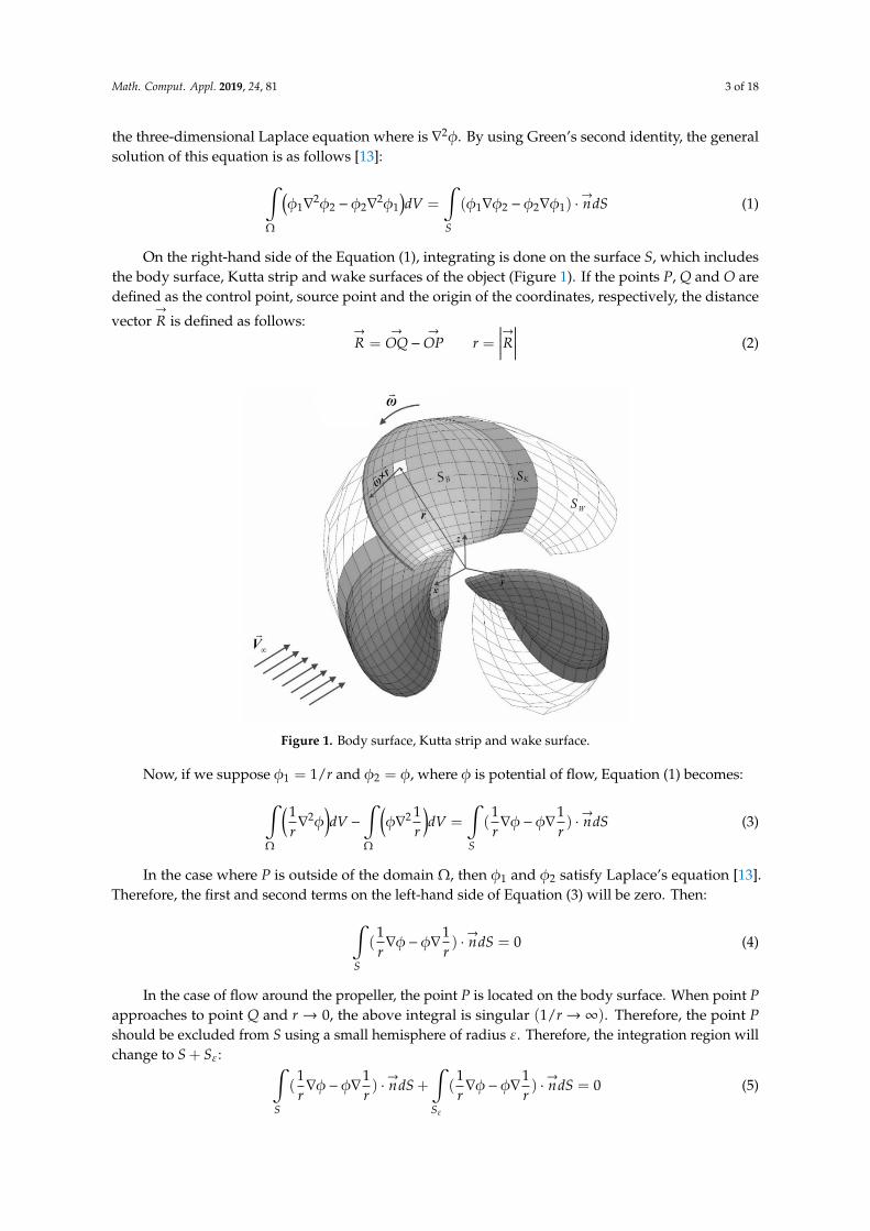
On the right-hand side of the Equation (1), integrating is done on the surface S, which includesthe body surface, Kutta strip and wake surfaces of the object (Figure 1). If the points P, Q and O aredefined as the control point, source point and the origin of the coordinates, respectively, the distance

vector→

R is defined as follows:→

R =→

OQ−→

OP r =∣∣∣∣∣→R∣∣∣∣∣ (2)

Math. Comput. Appl. 2019, 24, x FOR PEER REVIEW 4 of 18

Figure 1. Body surface, Kutta strip and wake surface.

Therefore, Equation (6) can written as below:

1 1 1 1 1 12 2

( ). ? ). ?

B K WS S S

P ndS ndSr r r r

(7)

The thickness of Kutta and wake surfaces are assumed to be zero. Then, .n for these surfaces

becomes zero. So:

1 1 1 1 12 2

( ). ? ?

B K WS S S

P ndS ndSr r r

(8)

This formulation is equivalent to distributing a source with strength of / n on each panel of the body surface and a doublet with strength of on each panel of the body surface, Kutta strip and wake surface. For greater simplicity, the strength of doublets on the Kutta strip and wake surface are displayed by µ . The final form of Equation (8) is as follows:

3 3 3

1 1 1 12 2 2 2

. . . .

B B K WS S S S

n n r n r n rP dS dS 礵 S 礵 Sr r r r

(9)

2.1. Boundary Conditions

Applying boundary conditions is one of the most important steps in solving problems by numerical methods. The first boundary condition that is applied is the non-entrance condition. If the propeller assumed to be rigid, the fluid particles cannot enter into the surface and the normal velocity will be zero on the surface of the propeller. If the propeller is operating in a uniform axial flow with velocity of

V and rotates with angular velocity of

, as shown in Figure 1, the total velocity of

point A on propeller blade is:

Av V r (10)

Then, the non-entrance condition for all panels of body surface is [14]:

1 . . 牋? ,A Bi in v n i N (11)

Then, Equation (9) becomes:

Figure 1. Body surface, Kutta strip and wake surface.

Now, if we suppose φ1 = 1/r and φ2 = φ, where φ is potential of flow, Equation (1) becomes:∫Ω

(1r∇

2φ)dV −

∫Ω

(φ∇2 1

r

)dV =

∫S

(1r∇φ−φ∇

1r) ·→ndS (3)

In the case where P is outside of the domain Ω, then φ1 and φ2 satisfy Laplace’s equation [13].Therefore, the first and second terms on the left-hand side of Equation (3) will be zero. Then:∫

S

(1r∇φ−φ∇

1r) ·→ndS = 0 (4)

In the case of flow around the propeller, the point P is located on the body surface. When point Papproaches to point Q and r → 0, the above integral is singular (1/r→∞). Therefore, the point Pshould be excluded from S using a small hemisphere of radius ε. Therefore, the integration region willchange to S + Sε: ∫

S

(1r∇φ−φ∇

1r) ·→ndS +

∫Sε

(1r∇φ−φ∇

1r) ·→ndS = 0 (5)


Using mathematical methods, the value of second integral is−2πφ(P). Then Equation (5) becomes:

φ(P) =1

2π

∫S

(1r∇φ−φ∇

1r) ·→ndS (6)

This equation gives the potential of flow (φ) at any point of body surface in terms of ∇φ andφ on the boundaries of domain. In Equation (6), the first and second terms of the integral can beinterpreted as a dipole with strength of φ and a source with strength of ∇φ, respectively. To expandthe above equation, as shown in Figure 1, the integration surface S is divided to body surface (SB),Kutta strip (SK), and wake surface (SW). Also, NB, NK and NW are number of panels on body surface,Kutta strip, and wake surface, respectively.

Therefore, Equation (6) can written as below:

φ(P) =1

2π

∫SB

(1r∇φ−φ∇

1r) ·→ndS +

12π

∫SK+SW

(1r∇φ−φ∇

1r) ·→ndS (7)

The thickness of Kutta and wake surfaces are assumed to be zero. Then, ∇φ ·→n for these surfaces

becomes zero. So:

φ(P) =1

2π

∫SB

(1r∇φ−φ∇

1r) ·→ndS−

12π

∫SK+SW

φ∇1r·→ndS (8)

This formulation is equivalent to distributing a source with strength of ∂φ/∂n on each panel ofthe body surface and a doublet with strength of φ on each panel of the body surface, Kutta strip andwake surface. For greater simplicity, the strength of doublets on the Kutta strip and wake surface aredisplayed by µ. The final form of Equation (8) is as follows:

φ(P) = −1

2π

∫SB

→n · ∇φ

rdS +

12π

∫SB

φ→n ·→r

r3 dS +1

2π

∫SK

µ→n ·→r

r3 dS +1

2π

∫SW

µ→n ·→r

r3 dS (9)

2.1. Boundary Conditions

Applying boundary conditions is one of the most important steps in solving problems by numericalmethods. The first boundary condition that is applied is the non-entrance condition. If the propellerassumed to be rigid, the fluid particles cannot enter into the surface and the normal velocity will bezero on the surface of the propeller. If the propeller is operating in a uniform axial flow with velocity

of→

V∞ and rotates with angular velocity of→ω, as shown in Figure 1, the total velocity of point A on

propeller blade is:→v A =

→

V∞ +→r ×

→ω (10)

Then, the non-entrance condition for all panels of body surface is [14]:(∇φ ·

→n)i=

(→v A ·

→n)ii = 1, . . . , NB (11)

Then, Equation (9) becomes:

φ(P) = −1

2π

∫SB

→v A ·

→n

rdS +

12π

∫SB

φ→n ·→r

r3 dS +1

2π

∫SK

µ→n ·→r

r3 dS +1

2π

∫SW

µ→n ·→r

r3 dS (12)


We can rewrite the above equation in series form as follows:

φi +NB∑

j = 1i , j

Ai jφ j +NK∑j=1

Ai jµ j =NB∑j=1

Bi j(→v A ·

→n)

j−

NW∑j=1

Ai jµ j i = 1, . . . , NB

Ai j = −1

2π

∫panel j

→n ·→

PQ∣∣∣∣∣ →PQ∣∣∣∣∣3 ds

Bi j = −1

2π

∫panel j

1∣∣∣∣∣ →PQ∣∣∣∣∣ds

(13)

where the points P and Q are assumed to be the center of panel i and j, respectively. Aij and Bijare known as influence coefficients and can be calculated according to Delhommeau [15]. The firstand second terms in right-hand side of Equation (13) are obtained from non-entrance boundarycondition and from previous time step, respectively. Therefore, the unknowns of the above equationare the strength of doublets on body panels and doublets on Kutta strip, hence NB + NK unknowns.Another boundary condition that is used to solve this problem is the Kutta condition. This conditionfor lifting bodies states that the flow should leave trailing edge smoothly and the velocity of flow therebe finite [13]. One of the best ways to apply this condition is presented by Morino [16]:

µi = (φi)u− (φi)

l i = 1, . . . , NK (14)

This means that strength of Kutta strip doublets is equal to difference of strength of upper (φ)u

and lower (φ)l doublets. Equation (13) will give NB equations and NK equations will be added tosystem of equations by applying Kutta condition. Finally, by solving this set of NB + NK equations,all NB + NK unknowns will be obtained.

2.2. Hydrodynamic Forces

After the calculation of velocity potential, the total velocity on each panel can be calculated usingnumerical differentiation methods. Then, the unsteady Bernoulli’s equation was used for calculationof total pressure [17]:

p− p∞ρ

= −12

∣∣∣∣∣ →∇φ−→v A

∣∣∣∣∣2 + 12

∣∣∣∣→v A

∣∣∣∣2 − ∂φ∂t(15)

where→

∇φ and ∂φ/∂t denote the surface gradient and time derivate of velocity potential. Propellerthrust can be calculated by integration of pressure forces on panels of propeller surface. Also, viscousforces should be obtained by using empirical formulas for surface friction coefficient (CD) of eachpanel [18]:

CD =0.0986(

log10 Rel − 1.22)2 (16)

where Rel is local Reynolds number based on radial location of panel (xr) and is Uxr/v. The viscousdrag of each panel is calculated as below [17]:

→

FD =12ρ ·CD ·

∣∣∣∣→v tot

∣∣∣∣→v tot (17)


where→v tot =

→v +

→v re f and

→v re f = −

→v A. Also,

→v is blade surface perturbation velocity and can be

obtained by taking surface gradient of velocity potential on blade panels. Then, total force and torqueof propeller are obtained as [19]:

→

F =∫(p ·

→n +

→

FD)dS→

M =∫ →

r × (p ·→n +

→

FD)dS(18)

Flowchart of panel method for calculation of hydrodynamic coefficient of propeller is shown inFigure 2. Initially, geometry of propeller and panels are generated by a function. A Kutta strip isalso created due to geometric considerations, propeller rotation and flow velocity. In the next step,a function calculates the influence coefficients for the sources and doublets. Then, the systems oflinear equations of Equation (13) is formed and then solved using iterative methods. By solving theequations, the velocity potential is obtained on the panels of body surface. With numerical derivationof potentials, velocity and pressure and on each panel are calculated and hydrodynamic coefficients ofpropeller are obtained. This process repeated until the solution converges. In this flowchart,

→v m is

the mean perturbation velocity of the points located on wake and Kutta surface. If these points arelocated in Xold position in time t, new position (Xnew) of points in time t + dt can be obtained using thefollowing equation:

Xnew = Xold +→v m · dt (19)

where→v m is calculated as below [19]:

→v m =

14π

∑SB

(→n ·→v A)

→rr3 dS +

14π

∑SB

φ

→

dl×→r

r3 +1

4π

∑SW+SK

µ

→

dl×→r

r3 (20)


where

tot refv v v and

ref Av v . Also, v is blade surface perturbation velocity and can be

obtained by taking surface gradient of velocity potential on blade panels. Then, total force and torque of propeller are obtained as [19]:

( . )?

( . )?D

D

F p n F dS

M r p n F dS (18)

Flowchart of panel method for calculation of hydrodynamic coefficient of propeller is shown in Figure 2. Initially, geometry of propeller and panels are generated by a function. A Kutta strip is also created due to geometric considerations, propeller rotation and flow velocity. In the next step, a function calculates the influence coefficients for the sources and doublets. Then, the systems of linear equations of Equation (13) is formed and then solved using iterative methods. By solving the equations, the velocity potential is obtained on the panels of body surface. With numerical derivation of potentials, velocity and pressure and on each panel are calculated and hydrodynamic coefficients of propeller are obtained. This process repeated until the solution converges. In this flowchart,

mv is

the mean perturbation velocity of the points located on wake and Kutta surface. If these points are located in oldX position in time t, new position ( )newX of points in time t + dt can be obtained using the following equation:

.new old mX X v dt (19)

where

mv is calculated as below [19]:

3 3 3

1 1 14 4 4

( . )

B B W K

m AS S S S

r dl r dl rv n v dSr r r

(20)

Figure 2. Flowchart of panel method. Figure 2. Flowchart of panel method.


3. Validation of Results of Panel Method

One of the most common propellers that has been used for the validation of numerical methods isthe DTMB 4119 propeller. This propeller is shown in Figure 3. Also, the main particulars and details ofgeometry are given in Tables 1 and 2, respectively.


3. Validation of Results of Panel Method

One of the most common propellers that has been used for the validation of numerical methods is the DTMB 4119 propeller. This propeller is shown in Figure 3. Also, the main particulars and details of geometry are given in Tables 1 and 2, respectively.

Figure 3. DTMB 4119 propeller.

Table 1. Main Particulars of DTMB 4119 Propeller [20].

3 Number of Blades 0.20 m Diameter

NACA 66 modified (a = 0.8) Blade Sections Profile 0.833 Design Advance Ratio (J)

Table 2. Geometry of DTMB 4119 Propeller [20].

r/R c/D P/D Skew Rake tmax/c fmax/c 0.2 0.3200 1.1050 0 0 0.2055 0.0143 0.3 0.3635 1.1022 0 0 0.1553 0.0232 0.4 0.4048 1.0983 0 0 0.1180 0.023 0.5 0.4392 1.0932 0 0 0.0916 0.0218 0.6 0.4610 1.0879 0 0 0.0696 0.0207 0.7 0.4622 1.0839 0 0 0.0542 0.0200 0.8 0.4347 1.0811 0 0 0.0421 0.0197 0.9 0.3613 1.0785 0 0 0.0332 0.0182

0.95 0.2775 1.0770 0 0 0.0323 0.0163 1 0.0800 1.0750 0 0 0.0316 0.0118

P is propeller pitch, r is radius of each section, R is propeller radius, c is chord of each section, D is propeller diameter, tmax is Maximum thickness of each section and fmax is maximum camber. For the validation of the results of numerical modeling for hydrodynamics and noise of DTMB 4119 propeller, some experiments were carried out with a model propeller in a cavitation tunnel of the Marine Engineering Laboratory of Sharif University of Technology (Figure 4). For measuring the thrust and torque of propeller model, a H29 dynamometer has been used in this tunnel.

Figure 3. DTMB 4119 propeller.

Table 1. Main Particulars of DTMB 4119 Propeller [20].

Number of Blades 3Diameter 0.20 m

Blade Sections Profile NACA 66 modified (a = 0.8)Design Advance Ratio (J) 0.833

Table 2. Geometry of DTMB 4119 Propeller [20].

r/R c/D P/D Skew Rake tmax/c fmax/c

0.2 0.3200 1.1050 0 0 0.2055 0.01430.3 0.3635 1.1022 0 0 0.1553 0.02320.4 0.4048 1.0983 0 0 0.1180 0.0230.5 0.4392 1.0932 0 0 0.0916 0.02180.6 0.4610 1.0879 0 0 0.0696 0.02070.7 0.4622 1.0839 0 0 0.0542 0.02000.8 0.4347 1.0811 0 0 0.0421 0.01970.9 0.3613 1.0785 0 0 0.0332 0.0182

0.95 0.2775 1.0770 0 0 0.0323 0.01631 0.0800 1.0750 0 0 0.0316 0.0118

P is propeller pitch, r is radius of each section, R is propeller radius, c is chord of each section,D is propeller diameter, tmax is Maximum thickness of each section and fmax is maximum camber.For the validation of the results of numerical modeling for hydrodynamics and noise of DTMB 4119propeller, some experiments were carried out with a model propeller in a cavitation tunnel of theMarine Engineering Laboratory of Sharif University of Technology (Figure 4). For measuring the thrustand torque of propeller model, a H29 dynamometer has been used in this tunnel.



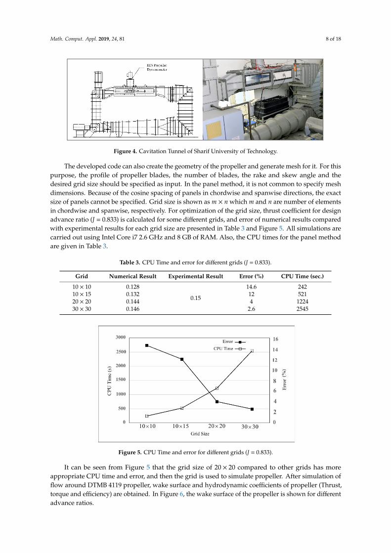
Figure 4. Cavitation Tunnel of Sharif University of Technology.

The developed code can also create the geometry of the propeller and generate mesh for it. For this purpose, the profile of propeller blades, the number of blades, the rake and skew angle and the desired grid size should be specified as input. In the panel method, it is not common to specify mesh dimensions. Because of the cosine spacing of panels in chordwise and spanwise directions, the exact size of panels cannot be specified. Grid size is shown as m × n which m and n are number of elements in chordwise and spanwise, respectively. For optimization of the grid size, thrust coefficient for design advance ratio (J = 0.833) is calculated for some different grids, and error of numerical results compared with experimental results for each grid size are presented in Table 3 and Figure 5. All simulations are carried out using Intel Core i7 2.6 GHz and 8 GB of RAM. Also, the CPU times for the panel method are given in Table 3.

Table 3. CPU Time and error for different grids (J = 0.833).

CPU Time (sec.) Error (%) Experimental Result Numerical Result Grid 242 14.6

0.15

0.128 10 × 10 521 12 0.132 10 × 15

1224 4 0.144 20 × 20 2545 2.6 0.146 30 × 30

Figure 5. CPU Time and error for different grids (J = 0.833).

It can be seen from Figure 5 that the grid size of 20 20 compared to other grids has more appropriate CPU time and error, and then the grid is used to simulate propeller. After simulation of flow around DTMB 4119 propeller, wake surface and hydrodynamic coefficients of propeller (Thrust, torque and efficiency) are obtained. In Figure 6, the wake surface of the propeller is shown for different advance ratios.


The developed code can also create the geometry of the propeller and generate mesh for it. For thispurpose, the profile of propeller blades, the number of blades, the rake and skew angle and thedesired grid size should be specified as input. In the panel method, it is not common to specify meshdimensions. Because of the cosine spacing of panels in chordwise and spanwise directions, the exactsize of panels cannot be specified. Grid size is shown as m × n which m and n are number of elementsin chordwise and spanwise, respectively. For optimization of the grid size, thrust coefficient for designadvance ratio (J = 0.833) is calculated for some different grids, and error of numerical results comparedwith experimental results for each grid size are presented in Table 3 and Figure 5. All simulations arecarried out using Intel Core i7 2.6 GHz and 8 GB of RAM. Also, the CPU times for the panel methodare given in Table 3.


Grid Numerical Result Experimental Result Error (%) CPU Time (sec.)

10 × 10 0.128

0.15

14.6 24210 × 15 0.132 12 52120 × 20 0.144 4 122430 × 30 0.146 2.6 2545



The developed code can also create the geometry of the propeller and generate mesh for it. For this purpose, the profile of propeller blades, the number of blades, the rake and skew angle and the desired grid size should be specified as input. In the panel method, it is not common to specify mesh dimensions. Because of the cosine spacing of panels in chordwise and spanwise directions, the exact size of panels cannot be specified. Grid size is shown as m × n which m and n are number of elements in chordwise and spanwise, respectively. For optimization of the grid size, thrust coefficient for design advance ratio (J = 0.833) is calculated for some different grids, and error of numerical results compared with experimental results for each grid size are presented in Table 3 and Figure 5. All simulations are carried out using Intel Core i7 2.6 GHz and 8 GB of RAM. Also, the CPU times for the panel method are given in Table 3.


CPU Time (sec.) Error (%) Experimental Result Numerical Result Grid 242 14.6

0.15

0.128 10 × 10 521 12 0.132 10 × 15

1224 4 0.144 20 × 20 2545 2.6 0.146 30 × 30


It can be seen from Figure 5 that the grid size of 20 20 compared to other grids has more appropriate CPU time and error, and then the grid is used to simulate propeller. After simulation of flow around DTMB 4119 propeller, wake surface and hydrodynamic coefficients of propeller (Thrust, torque and efficiency) are obtained. In Figure 6, the wake surface of the propeller is shown for different advance ratios.


It can be seen from Figure 5 that the grid size of 20 × 20 compared to other grids has moreappropriate CPU time and error, and then the grid is used to simulate propeller. After simulation offlow around DTMB 4119 propeller, wake surface and hydrodynamic coefficients of propeller (Thrust,torque and efficiency) are obtained. In Figure 6, the wake surface of the propeller is shown for differentadvance ratios.

Math. Comput. Appl. 2019, 24, 81 9 of 18Math. Comput. Appl. 2019, 24, x FOR PEER REVIEW 9 of 18

( 0.833)J ( 0.7)J ( 0.5)J

Figure 6. Wake surface of propeller for different advance ratios.

As shown in Figure 6, in low advance ratios which ship speed is low and propeller load is high (heavy duty conditions of propeller), disks of wake surface are closer together and wake rollup is intense but in higher advance ratios, disks of wake surface are more spacious and rollup is very low. Numerical simulation of propeller is performed by developed code for various advance ratios and Figure 7 compares the hydrodynamic coefficients of the propeller obtained by the panel method with experimental data.

Figure 7. Hydrodynamic coefficients of DTMB 4119 propeller.

The pressure distribution in the advance ratio of 0 833 .J for different radial sections of the propeller blade is compared with experimental measurements [21] in Figure 8.


As shown in Figure 6, in low advance ratios which ship speed is low and propeller load is high(heavy duty conditions of propeller), disks of wake surface are closer together and wake rollup isintense but in higher advance ratios, disks of wake surface are more spacious and rollup is very low.Numerical simulation of propeller is performed by developed code for various advance ratios andFigure 7 compares the hydrodynamic coefficients of the propeller obtained by the panel method withexperimental data.


( 0.833)J ( 0.7)J ( 0.5)J


As shown in Figure 6, in low advance ratios which ship speed is low and propeller load is high (heavy duty conditions of propeller), disks of wake surface are closer together and wake rollup is intense but in higher advance ratios, disks of wake surface are more spacious and rollup is very low. Numerical simulation of propeller is performed by developed code for various advance ratios and Figure 7 compares the hydrodynamic coefficients of the propeller obtained by the panel method with experimental data.


The pressure distribution in the advance ratio of 0 833 .J for different radial sections of the propeller blade is compared with experimental measurements [21] in Figure 8.


The pressure distribution in the advance ratio of J = 0.833 for different radial sections of thepropeller blade is compared with experimental measurements [21] in Figure 8.



(a) (b)

Figure 8. Experimental and panel method results for pressure distribution at (a) r/R = 0.3 and (b) r/R = 0.7.

According to Figure 7, there is satisfactory agreement between the hydrodynamic coefficients obtained from the panel method and experimental results. The maximum error of the trust coefficient calculated by the panel method is about 4% and for torque coefficient is about 7%. As can be seen in Figure 8, pressure distribution obtained from the panel method is in good agreement with the experimental data. This shows that the accuracy of the panel method results is acceptable. One reason for the greater error of the torque coefficient is the use of empirical formulas in the calculation of the friction resistance of each panel. According to the above results, the panel method can be used for hydrodynamic performance analysis of marine propellers.

4. Acoustic Formulations

In most acoustic problems, rigid bodies located in the fluid flow have very important effects on the generated noise. For this reason, Williams and Hawkings [22] in 1969 developed the Lighthill equations [23] with the assumption of rigid bodies. The equations presented by these researchers in acoustic science are known as the FW-H model. For solving the FW-H equation, Farassat et al. [24] presented a method that can predict the generated noise of moving object with arbitrary geometry. According to this formulation, total sound pressure can '( )p expressed as below [24]:

, ' , ' ,T Lp x t p x t p x t (21)

where 'Tp and 'Lp denote the thickness and loading pressure, respectively. Thickness pressure is due to the fluid displacement caused by movement of the body within the fluid and classified as monopole noise source. Another phenomenon caused by the motion of the non-symmetric body in fluid is the distribution of positive and negative pressure on the face and back of the body. In fact, this pressure distribution is the main source of trust force in propellers. Pressure difference on both sides of the body create a dipole noise source which is referred as loading pressure. This solution is obtained with assumption of low Mach number, and hence the quadrupole noise can be neglected. These components are calculated through the following relations [24]:

Figure 8. Experimental and panel method results for pressure distribution at (a) r/R = 0.3 and (b) r/R = 0.7.

According to Figure 7, there is satisfactory agreement between the hydrodynamic coefficientsobtained from the panel method and experimental results. The maximum error of the trust coefficientcalculated by the panel method is about 4% and for torque coefficient is about 7%. As can be seenin Figure 8, pressure distribution obtained from the panel method is in good agreement with theexperimental data. This shows that the accuracy of the panel method results is acceptable. One reasonfor the greater error of the torque coefficient is the use of empirical formulas in the calculation of thefriction resistance of each panel. According to the above results, the panel method can be used forhydrodynamic performance analysis of marine propellers.

4. Acoustic Formulations

In most acoustic problems, rigid bodies located in the fluid flow have very important effects onthe generated noise. For this reason, Williams and Hawkings [22] in 1969 developed the Lighthillequations [23] with the assumption of rigid bodies. The equations presented by these researchers inacoustic science are known as the FW-H model. For solving the FW-H equation, Farassat et al. [24]presented a method that can predict the generated noise of moving object with arbitrary geometry.According to this formulation, total sound pressure can (p′) expressed as below [24]:

p′(→x , t

)= p′T

(→x , t

)+ p′L

(→x , t

)(21)

where p′T and p′L denote the thickness and loading pressure, respectively. Thickness pressure is due tothe fluid displacement caused by movement of the body within the fluid and classified as monopolenoise source. Another phenomenon caused by the motion of the non-symmetric body in fluid is thedistribution of positive and negative pressure on the face and back of the body. In fact, this pressuredistribution is the main source of trust force in propellers. Pressure difference on both sides of thebody create a dipole noise source which is referred as loading pressure. This solution is obtained withassumption of low Mach number, and hence the quadrupole noise can be neglected. These componentsare calculated through the following relations [24]:

4πp′T(→x , t

)=

∫S

[ρ(

.vn+v .

n)

r(1−Mr)2

]ret

dS +∫S

[ρvn

(r

.Mr+cMr−cM2

)r2(1−Mr)

3

]ret

dS

4πp′L(→x , t

)= 1

c

∫S

[ .Lr

r(1−Mr)2

]ret

dS + 1c

∫S

[Lr−LM

r2(1−Mr)2

]ret

dS

+ 1c

∫S

[Lr

(r

.Mr+cMr−cM2

)r2(1−Mr)

3

]ret

dS

(22)


where ρ is fluid density in kg/m3, c is sound speed in m/s,→v is the noise source velocity in m/s,

→r is

distance vector from noise source to receiver in m, r is magnitude of→r in m, Mach number is

→

M =→v /c,

L = p ·→n is pressure force in N and p is hydrodynamic pressure in Pa. The dot over variables means

time derivate of the variable. The ret subscript in this equation means that the calculations must bedone using values at the retarded time.

In the first step of noise calculation, the flow around the body is simulated using the panelmethod and flow quantities such as pressure and velocity are obtained for panels on the body surface.Then, for receiver in position of

→x and time of ti, retarded time (τi, j) is obtained for panel j. After this

step, all quantities required in Equation (20) must be calculated for each panel at the retarded time,numerical integrals of the equation are solved for each panel, and the acoustic pressure of each elementis obtained. By summing up the acoustic pressures of all the elements, a total acoustic pressure isobtained for the specified receiver. Flowchart of noise calculation using FW-H equations is shown inFigure 9.


2

2 32

2 22

41 1

1 141 1

'

'

( ),

, 牋?

n r rn nT

S Sr rret ret

r ML

S Sr rret ret

r

v rM cM cMv vp x t dS dS

r M r M

L Lp x t dS dS

c M

Lcr r M

2

32

1

1

牋 ?r r r

S r ret

L rM cM cMdS

c r M

(22)

where ρ is fluid density in 3?kg m , c is sound speed in ? sm , v is the noise source velocity in ? sm

, r is distance vector from noise source to receiver in m , r is magnitude of r in m , Mach

number is /M v c ,

.L p n is pressure force in N and p is hydrodynamic pressure in 燩a . The dot over variables means time derivate of the variable. The ret subscript in this equation means that the calculations must be done using values at the retarded time.

In the first step of noise calculation, the flow around the body is simulated using the panel method and flow quantities such as pressure and velocity are obtained for panels on the body surface. Then, for receiver in position of x and time of ti, retarded time ,( )i j is obtained for panel j. After

this step, all quantities required in Equation (20) must be calculated for each panel at the retarded time, numerical integrals of the equation are solved for each panel, and the acoustic pressure of each element is obtained. By summing up the acoustic pressures of all the elements, a total acoustic pressure is obtained for the specified receiver. Flowchart of noise calculation using FW-H equations is shown in Figure 9.

Figure 9. Flowchart of noise calculation using FW-H equations. Figure 9. Flowchart of noise calculation using FW-H equations.

5. Noise of DTMB 4119 Propeller

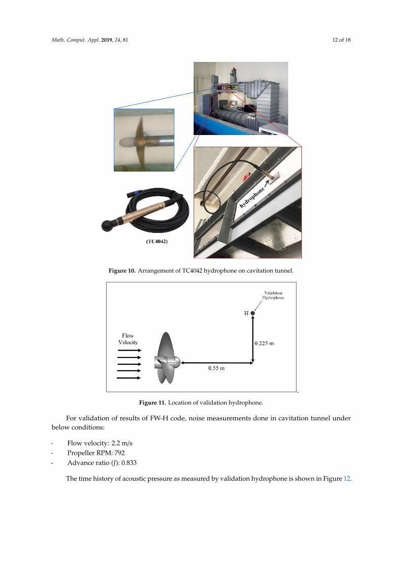
The noise generated by the propeller is one of the most important components of the vesselsnoise [6]. Therefore, measuring and calculating the propeller noise is one of the interesting researchsubjects in naval engineering. In the first step, the results of the developed FW-H code for noisecalculation should validated using experimental results obtained in cavitation tunnel. For measuringthe noise of propeller, a TC4042 hydrophone has been used in cavitation tunnel of Sharif University ofTechnology. The arrangement of this validation hydrophone is shown in Figure 10. Also, the locationof this hydrophone is given in Figure 11.




The noise generated by the propeller is one of the most important components of the vessels noise [6]. Therefore, measuring and calculating the propeller noise is one of the interesting research subjects in naval engineering. In the first step, the results of the developed FW-H code for noise calculation should validated using experimental results obtained in cavitation tunnel. For measuring the noise of propeller, a TC4042 hydrophone has been used in cavitation tunnel of Sharif University of Technology. The arrangement of this validation hydrophone is shown in Figure 10. Also, the location of this hydrophone is given in Figure 11.

Figure 10. Arrangement of TC4042 hydrophone on cavitation tunnel.

.

Figure 11. Location of validation hydrophone.




The noise generated by the propeller is one of the most important components of the vessels noise [6]. Therefore, measuring and calculating the propeller noise is one of the interesting research subjects in naval engineering. In the first step, the results of the developed FW-H code for noise calculation should validated using experimental results obtained in cavitation tunnel. For measuring the noise of propeller, a TC4042 hydrophone has been used in cavitation tunnel of Sharif University of Technology. The arrangement of this validation hydrophone is shown in Figure 10. Also, the location of this hydrophone is given in Figure 11.


.



For validation of results of FW-H code, noise measurements done in cavitation tunnel underbelow conditions:

- Flow velocity: 2.2 m/s- Propeller RPM: 792- Advance ratio (J): 0.833

The time history of acoustic pressure as measured by validation hydrophone is shown in Figure 12.



For validation of results of FW-H code, noise measurements done in cavitation tunnel under below conditions:

- Flow velocity: 2.2 m/s - Propeller RPM: 792 - Advance ratio (J): 0.833


Figure 12. Time history of acoustic pressure measured by validation hydrophone.

In the post-processing stage, acoustic pressure from time domain in transferred to frequency domain by using the fast Fourier transform (FFT) and the sound pressure level is calculated using the following formula [25]:

1020 , log / refSPL x t p p (23)

where refp is the reference pressure and related to threshold of a normal human hearing for

frequency of 1 kHz which for water is 1?μPa [26]. The numerical results of noise obtained by own developed code compared by experimental results in Figure 13. Propeller and flow conditions are the same as the experimental setup.

Figure 13. Validation of FW-H code results.


In the post-processing stage, acoustic pressure from time domain in transferred to frequencydomain by using the fast Fourier transform (FFT) and the sound pressure level is calculated using thefollowing formula [25]:

SPL(→x , t

)= 20 log10

(p′/pre f

)(23)

where pre f is the reference pressure and related to threshold of a normal human hearing for frequencyof 1 kHz which for water is 1 µPa [26]. The numerical results of noise obtained by own developedcode compared by experimental results in Figure 13. Propeller and flow conditions are the same as theexperimental setup.


For validation of results of FW-H code, noise measurements done in cavitation tunnel under below conditions:

- Flow velocity: 2.2 m/s - Propeller RPM: 792 - Advance ratio (J): 0.833



In the post-processing stage, acoustic pressure from time domain in transferred to frequency domain by using the fast Fourier transform (FFT) and the sound pressure level is calculated using the following formula [25]:

1020 , log / refSPL x t p p (23)

where refp is the reference pressure and related to threshold of a normal human hearing for

frequency of 1 kHz which for water is 1?μPa [26]. The numerical results of noise obtained by own developed code compared by experimental results in Figure 13. Propeller and flow conditions are the same as the experimental setup.

Figure 13. Validation of FW-H code results. Figure 13. Validation of FW-H code results.

It can be seen that there is good agreement between the numerical and experimental results ofpropeller noise, especially in frequencies under 250 Hz. It seems that main sources of error of numericalresults are:

- Error of panel method code for calculation of pressure and flow velocity: As mentioned in theprevious sections, the results of the thrust and torque of the panel method have 4% and 7%error in comparison with the experimental results. Since the FW-H equations use panel methodoutputs, the above error causes an error in calculating the noise of the impeller.

- The error of FW-H code for noise calculation: FW-H equations include some integrals that arecalculated numerically on the source of noise. Therefore, the numerical calculation error of these


equations can cause error in the value of noise. Also, in the solution presented in this study,the quadrupole sources of noise are neglected, which could cause a slight error in the value ofpropeller noise.

- The reflection of sound inside the cavitation tunnel is another reason for the difference betweenthe experimental and numerical results. The restricted space of the cavitation tunnel causes thereverberation of sound emitted by the propeller, which results in an error in the measured noisevalues. For investigating the effects of sound reverberation on noise data, special equipment isneeded which is not available in our laboratory.

Seol et al. [27] and Yang et al. [28] carried out some numerical studies on DTMB 4119 propeller,but since the specifications of the propeller used are not the same as the propeller model in ourlaboratory, the results cannot be compared.

By looking more precisely into results, it founds that both experimental and numerical resultshave peaks in some frequencies. It seems that these are Blade Passing Frequencies (BPF) of propeller.For the propeller, the rate at which the blades pass by a fixed position is called the BPF. This frequencyis known as the blade passing frequency (BPF) of the blade. As regards the propeller, the BPF and itshigher harmonics can be calculated as:

BPF = Z× rps× h (Hz) (24)

where Z is number of propeller blades, rps is the frequency of propeller rotation in Hz and h is no ofharmonic. When receiver is located in an asymmetric location relative to blades, the noise of propellerin BPFs will have local peaks in comparison to other frequencies. For the receiver, which is located inthe hub plane of the propeller, at an equal and constant distance from the blades at all times, BPF couldnot be seen in the SPL diagram. For noise diagrams in Figure 13, rps is 13.2 and Z is 3. Therefore, BPFfor three first harmonics of propeller is about 39.6, 79.2 and 118.8 Hz and noise results have peaks inthe first two frequencies.

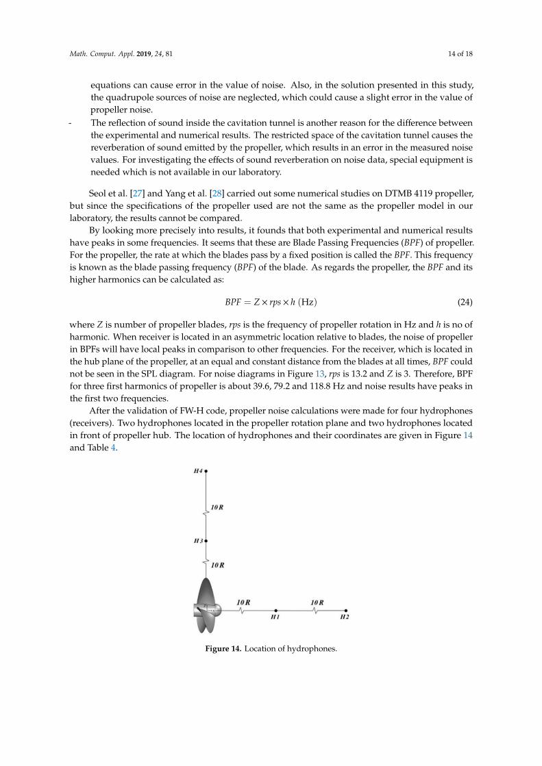
After the validation of FW-H code, propeller noise calculations were made for four hydrophones(receivers). Two hydrophones located in the propeller rotation plane and two hydrophones locatedin front of propeller hub. The location of hydrophones and their coordinates are given in Figure 14and Table 4.Math. Comput. Appl. 2019, 24, x FOR PEER REVIEW 15 of 18

Figure 14. Location of hydrophones.

Table 4. Coordinates of hydrophones.

X(m) Y(m) Z(m) H1 1 0 0 H2 2 0 0 H3 0 1 0 H4 0 2 0

The noise of the propeller as calculated by the FW-H code for hydrophones H1 and H2 are presented in Figure 15. Noise predictions were made at a flow speed of 2.2 m/s and RPM of 792 where J = 0.833.

Figure 15. Sound pressure level of propeller in hydrophones H1 and H2.




X(m) Y(m) Z(m)

H1 1 0 0H2 2 0 0H3 0 1 0H4 0 2 0

The noise of the propeller as calculated by the FW-H code for hydrophones H1 and H2 arepresented in Figure 15. Noise predictions were made at a flow speed of 2.2 m/s and RPM of 792 whereJ = 0.833.




X(m) Y(m) Z(m) H1 1 0 0 H2 2 0 0 H3 0 1 0 H4 0 2 0

The noise of the propeller as calculated by the FW-H code for hydrophones H1 and H2 are presented in Figure 15. Noise predictions were made at a flow speed of 2.2 m/s and RPM of 792 where J = 0.833.

Figure 15. Sound pressure level of propeller in hydrophones H1 and H2. Figure 15. Sound pressure level of propeller in hydrophones H1 and H2.

Results shown in Figure 15 reveals that by increasing the distance of hydrophone from propeller,noise of H2 decreased significantly in comparison with H1. Also, in Figure 16, the propeller noise inhydrophones H3 and H4 are presented.



Results shown in Figure 15 reveals that by increasing the distance of hydrophone from propeller, noise of H2 decreased significantly in comparison with H1. Also, in Figure 16, the propeller noise in hydrophones H3 and H4 are presented.


As can be seen in Figure 16, with an increase of distance from the propeller, noise decreased significantly. Also, in both hydrophones, at a blade passing frequency of 18.22 Hz, the noise has a peak value which is also indicated in the Figure 16. By comparing Figures 15 and 16, it can be seen that the SPL in front of the propeller hub is higher than the SPL in the propeller rotational plane.

6. Conclusions

Measuring and calculating the noise of marine propellers is very important. In this research, the combination of the panel method and FW-H equations has been used to calculate the non-cavitating noise of marine propellers. In the first step, a numerical panel method code is developed to solve the flow around the propeller and calculate the propeller hydrodynamic coefficients. The results of this code in comparison with the experimental results had maximum error of 4% and 7% for thrust and torque coefficients, respectively.

Then, a noise calculation code based on FW-H acoustic equations was developed, which uses the outputs of the panel method code as inputs and calculates the noise of the propeller for the desired receiver. The results of this code are in good agreement with the noise of the propeller obtained using results from a test carried out in cavitation tunnel of Sharif University. Using this code, the propeller noise is measured for four hydrophones with different distances and orientations. With increasing distance from the propeller, the noise of the propeller has been significantly reduced. For the hydrophones located on the rotation plane of the propeller, as predicted by theory and experiments on propeller noise, the maximum noise has occurred at the blade passing frequency. The results show that the SPL in front of the propeller hub is higher than SPL in the propeller rotational plane.

According to the above results, the combination of the panel method and FW-H equations can be used for hydrodynamic and acoustic analysis of marine propellers.

Author Contributions: All authors contributed equally in this work.

Funding: This research received no external funding.

Conflicts of Interest: The authors declare no conflict of interest.


As can be seen in Figure 16, with an increase of distance from the propeller, noise decreasedsignificantly. Also, in both hydrophones, at a blade passing frequency of 18.22 Hz, the noise has a peakvalue which is also indicated in the Figure 16. By comparing Figures 15 and 16, it can be seen that theSPL in front of the propeller hub is higher than the SPL in the propeller rotational plane.

6. Conclusions

Measuring and calculating the noise of marine propellers is very important. In this research,the combination of the panel method and FW-H equations has been used to calculate the non-cavitatingnoise of marine propellers. In the first step, a numerical panel method code is developed to solve theflow around the propeller and calculate the propeller hydrodynamic coefficients. The results of thiscode in comparison with the experimental results had maximum error of 4% and 7% for thrust andtorque coefficients, respectively.

Then, a noise calculation code based on FW-H acoustic equations was developed, which uses theoutputs of the panel method code as inputs and calculates the noise of the propeller for the desiredreceiver. The results of this code are in good agreement with the noise of the propeller obtained usingresults from a test carried out in cavitation tunnel of Sharif University. Using this code, the propellernoise is measured for four hydrophones with different distances and orientations. With increasingdistance from the propeller, the noise of the propeller has been significantly reduced. For thehydrophones located on the rotation plane of the propeller, as predicted by theory and experiments onpropeller noise, the maximum noise has occurred at the blade passing frequency. The results show thatthe SPL in front of the propeller hub is higher than SPL in the propeller rotational plane.

According to the above results, the combination of the panel method and FW-H equations can beused for hydrodynamic and acoustic analysis of marine propellers.

Author Contributions: All authors contributed equally in this work.

Funding: This research received no external funding.

Conflicts of Interest: The authors declare no conflict of interest.


References

1. Hess, J.L.; Smith, A.M.O. Calculation of Nonlifting Potential Flow about Arbitrary Three-Dimensional Bodies;Douglas Aircraft Co.: Long Beach, CA, USA, 1962.

2. Hess, J.L. Calculation of Potential Flow about Arbitrary Three-Dimensional Lifting Bodies; Douglas Aircraft Co.:Long Beach, CA, USA, 1972.

3. Hess, J.; Valarezo, W. Calculation of steady flow about propellers by means of a surface panel method.J. Propuls. Power 1985, 1, 470–476. [CrossRef]

4. Baltazar, J.M.R.D.C.; De Campos, J.A.C.F. An iteratively coupled solution of the cavitating flow on marinepropellers using BEM. J. Hydrodyn. 2010, 22, 796–801. [CrossRef]

5. Gaggero, S.; Villa, D.; Brizzolara, S. RANS and PANEL method for unsteady flow propeller analysis.J. Hydrodyn. 2010, 22, 547–552. [CrossRef]

6. Ebrahimi, A.; Razaghian, A.; Seif, M.; Zahedi, F.; Nouri-Borujerdi, A. A comprehensive study on noisereduction methods of marine propellers and design procedures. Appl. Acoust. 2019, 150, 55–69. [CrossRef]

7. Seol, H.; Park, C. Numerical and Experimental Study on the Marine Propeller Noise. In Proceedings of the19th International Congress on Acoustics, Madrid, Spain, 2–7 September 2007; pp. 2–7.

8. Kellett, P.; Turan, O.; Incecik, A. A study of numerical ship underwater noise prediction. Ocean Eng. 2013, 66,113–120. [CrossRef]

9. Bagheri, M.; Seif, M.; Mehdigholi, H. Numerical Simulation of underwater propeller noise. J. Ocean Mech.Aerosp. 2014, 4, 4–9.

10. Testa, C.; Ianniello, S.; Salvatore, F. A Ffowcs Williams and Hawkings formulation for hydroacoustic analysisof propeller sheet cavitation. J. Sound Vib. 2018, 413, 421–441. [CrossRef]

11. Gorji, M.; Ghassemi, H.; Mohamadi, J. Calculation of sound pressure level of marine propeller in lowfrequency. J. Low Freq. Noise Vib. Act. Control. 2018, 37, 60–73. [CrossRef]

12. Bagheri, M.R.; Seif, M.S.; Mehdigholi, H.; Yaakob, O. Analysis of noise behaviour for marine propellersunder cavitating and non-cavitating conditions. Ships Offshore Struct. 2017, 12, 1–8. [CrossRef]

13. Katz, J.; Plotkin, A. Low-Speed Aerodynamics; Cambridge University Press: Cambridge, UK, 2001.14. Politis, G. Unsteady Wake Rollup Modeling Using a Mollifier Based Filtering Technique. Dev. Appl. Ocean.

Eng. 2016, 5, 1. [CrossRef]15. Delhommeau, G. Amélioration des performances des codes de calcul de diffraction-radiation au premier

ordre. In Proceedings of the 2nd Journées de l’Hydrodynamique, Nantes, France, 13–15 February 1989.16. Morino, L.; Kuo, C. Subsonic potential aerodynamics for complex configurations: A general theory. AIAA J.

1974, 12, 191–197.17. Politis, G.K. Unsteady Rollup Modeling for Wake-Adapted Propellers Using a Time-Stepping Method. J. Ship

Res. 2005, 49, 216–231.18. Blevins, R.D. Applied Fluid Dynamics Handbook; Van Nostrand Reinhold Co.: New York, NY, USA, 1984; p. 568.19. Najafi, S.; Abbaspoor, M. Numerical investigation of flow pattern and hydrodynamic forces of submerged

marine propellers using unsteady boundary element method. Proc. Inst. Mech. Eng. Part M J. Eng. Marit.Environ. 2017, 233, 67–79. [CrossRef]

20. Boumediene, K.; Belhenniche, S. Numerical Analysis of the Turbulent Flow around DTMB 4119 MarinePropeller. Int. J. Mech. Aerosp. Ind. Mechatron. Manuf. Eng. 2016, 10, 347–351.

21. Jessup, S. An Experimental Investigation of Viscous Aspects of Propeller Blade Flow. Ph.D. Thesis,The Catholic University of America, Washington, DC, USA, 1989.

22. Williams, J.E.F.; Hawkings, D.L. Sound Generation by Turbulence and Surfaces in Arbitrary Motion. Philos.Trans. R. Soc. A Math. Phys. Eng. Sci. 1969, 264, 321–342. [CrossRef]

23. Lighthill, M.J. On sound generated aerodynamically II. Turbulence as a source of sound. Proc. R. Soc. Lond.Ser. A. Math. Phys. Sci. 1954, 222, 1–32.

24. Farassat, F. Derivation of Formulations 1 and 1A of Farassat; NASA Langley Research Center: Hampton, VA,USA, 2007.

25. Kinsler, L.A.; Frey, A.R.; Coppens, A.B.; Sanders, J.V. Fundamentals of Acoustics; John Wiley & Sons: New York,NY, USA, 2000.

26. Council, N.R. Low-Frequency Sound and Marine Mammals: Current Knowledge and Research Needs; NationalAcademies Press: Washington, DC, USA, 1994.

http://dx.doi.org/10.2514/3.22830

http://dx.doi.org/10.1016/S1001-6058(10)60039-X

http://dx.doi.org/10.1016/S1001-6058(09)60253-5

http://dx.doi.org/10.1016/j.apacoust.2018.12.004

http://dx.doi.org/10.1016/j.oceaneng.2013.04.006

http://dx.doi.org/10.1016/j.jsv.2017.10.004

http://dx.doi.org/10.1177/1461348418757884

http://dx.doi.org/10.1080/17445302.2015.1099224

http://dx.doi.org/10.14355/daoe.2016.05.001

http://dx.doi.org/10.1177/1475090217717174

http://dx.doi.org/10.1098/rsta.1969.0031


27. Seol, H.; Suh, J.-C.; Lee, S. Development of hybrid method for the prediction of underwater propeller noise.J. Sound Vib. 2005, 288, 345–360. [CrossRef]

28. Yang, Q.; Wang, Y.; Zhang, M. Calculation of propeller’s load noise using LES and BEM numerical acousticscoupling methods. WIT Trans. Model. Simul. Bound. Elem. Other Reduct. Methods XXXIII 2011, 52, 85–97.

© 2019 by the authors. Licensee MDPI, Basel, Switzerland. This article is an open accessarticle distributed under the terms and conditions of the Creative Commons Attribution(CC BY) license (http://creativecommons.org/licenses/by/4.0/).

http://dx.doi.org/10.1016/j.jsv.2005.01.015

http://creativecommons.org/

http://creativecommons.org/licenses/by/4.0/.

hydrodynamic and acoustic performance analysis of marine

Documents