hydraulic tomography: development of a new...

Hydraulic tomography:Development of a new aquifer test methodT.-C. Jim Yeh and Shuyun LiuDepartment of Hydrology and Water Resources, University of Arizona, Tucson

Abstract. Hydraulic tomography (i.e., a sequential aquifer test) has recently beenproposed as a method for characterizing aquifer heterogeneity. During a hydraulictomography experiment, water is sequentially pumped from or injected into an aquifer atdifferent vertical portions or intervals of the aquifer. During each pumping or injection,hydraulic head responses of the aquifer at other intervals are monitored, yielding a set ofhead/discharge (or recharge) data. By sequentially pumping (or injecting) water at oneinterval and monitoring the steady state head responses at others, many head/discharge(recharge) data sets are obtained. In this study a sequential inverse approach is developedto interpret results of hydraulic tomography. The approach uses an iterative geostatisticalinverse method to yield the effective hydraulic conductivity of an aquifer, conditioned oneach set of head/discharge data. To efficiently include all the head/discharge data sets, asequential conditioning method is employed. It uses the estimated hydraulic conductivityfield and covariances, conditioned on the previous head/discharge data set, as priorinformation for next estimations using a new set of pumping data. This inverse approachwas first applied to hypothetical, two-dimensional, heterogeneous aquifers to investigatethe optimal sampling scheme for the hydraulic tomography, i.e., the design of well spacing,pumping, and monitoring locations. The effects of measurement errors and uncertaintiesin statistical parameters required by the inverse model were also investigated. Finally, therobustness of this inverse approach was demonstrated through its application to ahypothetical, three-dimensional, heterogeneous aquifer.

1. Introduction

Accurate predictions of water and solute distributions andmovement in geological formations require detailed knowl-edge of the spatial distribution of the hydraulic properties ofthe formations [Yeh, 1992, 1998]. Conventional aquifer tests(also known as pumping tests) assume aquifer homogeneityand yield effective hydraulic conductivity and the storage co-efficient for an equivalent homogeneous aquifer. These hy-draulic parameters are average properties of the aquifer over alarge volume [Butler and Liu, 1993] and do not provide infor-mation of spatial distribution of the hydraulic conductivitywithin the volume. On the other hand, measurement of hy-draulic conductivity of small-scale samples at a large number oflocations is time-consuming, costly, and impractical.

To circumvent these difficulties and to efficiently gain infor-mation of the spatial distribution of hydraulic conductivity, thegeophysical tomography concept has recently been employed[Gottlieb and Dietrich, 1995; Butler et al., 1999]. Specifically,fully screened wells are segregated into many vertical intervalsusing packers. Water is pumped from or injected into an aqui-fer at one of the intervals to create a steady flow condition.Hydraulic head responses of the aquifer at other intervals arethen monitored, yielding a set of head/discharge (or recharge)data. By sequentially pumping (or injecting) water at one in-terval and monitoring the steady state head response at others,many head/discharge (or recharge) data sets are obtained.Such a sequential aquifer test is referred to as hydraulic to-mography. This new field method has significant advantages

over traditional pumping tests. For instance, hydraulic tomog-raphy can provide detailed information about vertical and lat-eral pressure head responses induced by pumping at a givenlocation. Furthermore, by changing the position of the pump inthe well, many sets of aquifer responses to pumping at differ-ent locations can be obtained. Such a large number of data setsmay reduce the nonuniqueness issue of the inverse problemand may reveal the details of a heterogeneous hydraulic con-ductivity field.

Several researchers have recently investigated this idea ofhydraulic tomography. For example, Gottlieb and Dietrich[1995] proposed a method of hydraulic tomography for iden-tifying the permeability distribution in a hypothetical, two-dimensional saturated soil. In their study they used two bore-holes to create hydraulic dipoles. The positions of source andsink are varied over both boreholes. Pore water pressurechanges along the vertical were monitored in monitoring wellsat other locations. They subsequently applied a least squares–based inverse approach to the pressure data to produce animage of the spatial distribution of hydraulic conductivity. But-ler et al. [1999] applied this hydraulic tomography concept tonetworks of multilevel sampling wells. They developed newtechniques for measuring drawdown data at a scale that hadpreviously been unobtainable. These new techniques greatly fa-cilitate the implementation of hydraulic tomography in the field.

Hydraulic tomography can yield many useful sets of second-ary information, namely head responses, that can be used toidentify heterogeneity of the aquifer. Still, a reliable and effi-cient inverse methodology is required to decipher the infor-mation so that a reliable image of the hydraulic conductivityfield can be obtained. Classical inverse methodologies areknown to have many difficulties [Yeh, 1986]. They also confront

Copyright 2000 by the American Geophysical Union.

Paper number 2000WR900114.0043-1397/00/2000WR900114$09.00

WATER RESOURCES RESEARCH, VOL. 36, NO. 8, PAGES 2095–2105, AUGUST 2000

2095

an insurmountable computational burden when they are ap-plied to estimate detailed hydraulic properties in three-dimensional geological formations [Kitanidis, 1997]. Conse-quently, few classical inverse models have been applied toidentify small-scale heterogeneity in three-dimensional geolog-ical media. More importantly, the abundance of hydraulic headinformation generated by hydraulic tomography presents aneven greater challenge for the classical inverse methodologies.

In the past few decades, cokriging has been used to estimatehydraulic conductivity fields from scattered measurements ofpressure head in saturated flow problems [Kitanidis and Vom-voris, 1983; Hoeksema and Kitanidis, 1984]. However, cokrigingis a linear estimator, and its application is limited to mildlynonlinear systems, such as groundwater flow in geological for-mations of mild heterogeneity (variance of natural log of con-ductivity slnk

2 5 0.1). When the degree of aquifer heterogeneityis large (slnk

2 . 1) and the linear assumption becomes inade-quate, cokriging cannot provide a good estimate of the condi-tional mean conductivity field [Yeh et al., 1996]. In other words,it cannot take full advantage of the head information to obtainan optimal estimate of the hydraulic properties.

To overcome this shortcoming, Yeh et al. [1995, 1996] andZhang and Yeh [1997] developed an iterative geostatisticaltechnique in which a linear estimator was used successively toincorporate the nonlinear relationship between hydraulicproperties and pressure head. This method is referred to as asuccessive linear estimator (SLE). They demonstrated thatwith the same amount of information the SLE revealed a moredetailed conductivity field than cokriging. Hughson and Yeh[1998, 2000] showed that the SLE is computationally efficientcompared to the classical inverse method. They extended it tothe inverse problem in three-dimensional, variably saturated,heterogeneous porous media, which had not been attemptedbefore. In their study, pressure head and moisture contentmeasurements at 42 locations (7 wells 3 6 depths) in a three-dimensional porous medium were collected at three differenttimes during an infiltration event. This secondary informationwas then used to estimate saturated hydraulic conductivity Ks

and a parameter of the Mualem-van Genuchten unsaturatedhydraulic property model [van Genuchten, 1980] at 500 loca-tions in the porous medium.

In this paper, on the basis of the SLE we develop a sequen-tial inverse technique for hydraulic tomography to process thelarge amount of data to characterize aquifer heterogeneity.While demonstrating the robustness of the inverse method, wealso investigate the effect of monitoring intervals, pumpingintervals, and the number of pumping locations on the finalestimate of hydraulic conductivity. Guidelines for optimal de-sign of a hydraulic tomography test are subsequently estab-lished. To further verify our results, Monte Carlo inverse sim-ulations are performed, and the effects of measurement errorsand uncertainties in statistical parameters required by the in-verse model are investigated. Finally, an example is used toillustrate the effectiveness and the robustness of this sequentialapproach for hydraulic tomography under three-dimensional,steady flow conditions.

2. Methodology2.1. Equation of Flow in Three-DimensionalSaturated Media

In this study we assume that the steady state flow field,created by the hydraulic tomography in three-dimensional, sat-

urated, heterogeneous, porous media can be described by thefollowing equation:

¹ ? @K~x!¹f# 1 Q~x! 5 0 (1)

with boundary conditions

f uG1 5 f*, @K~x!¹f# ? n uG2 5 q , (2)

where f is total head (m), x is the spatial coordinate (x 5 { x1,x2, x3}, m, and x3 represents the vertical coordinate and ispositive upward), Q is the pumping rate (m3/h m3) at theselected interval during the tomography experiment, and K(x)is the saturated hydraulic conductivity field in m/h. In (2),prescribed total head on the Dirichlet boundary G1 is denotedby f* (m). Specified flux q , in m/h, is given on the Neumannboundary conditions G2, and n is a unit vector normal to theunion of G1 and G2.

2.2. Sequential Inverse Algorithm

To deal with aquifer heterogeneity, the natural log of hy-draulic conductivity, ln (K(x)), of an aquifer is treated as astationary stochastic process with an unconditional mean, ^lnK& 5 F (the angle brackets denote the expected value), andthe unconditional perturbation f . The corresponding steadyhydraulic head distribution due to pumping in an interval inthe hydraulic tomography is then presented by f(x) 5 H(x) 1h(x), where H 5 ^f& and h is the unconditional head pertur-bation. Suppose that we have used well log data and coresamples to determine nf conductivity values f*i 5 (ln K*i 2 F),where i 5 1, 2, z z z , nf (we will refer to these data sets asprimary information). Additionally, we have estimated themean and correlation structure of the conductivity field. Alsoassume that during a hydraulic tomography experiment wehave collected m sets of nh observed head values f*j, wherej 5 nf 1 1, nf 1 2, z z z , nf 1 mnh during m sequentialpumping tests. These head data sets are referred to as second-ary information. We then seek an inverse model that can pro-duce head and conductivity fields that preserve the observedhead and conductivity values at sample locations and satisfytheir underlying statistical properties (i.e., mean and covari-ance, etc.) and the governing flow equation. In the conditionalprobability concept, such a head or conductivity field is a con-ditional realization of f or ln K field among many possiblerealizations of the ensemble. Consequently, a conditional con-ductivity field can be expressed as the sum of conditional meanconductivity and its conditional perturbation, Kc(x) 5 ^Kc(x)& 1kc(x). Similarly, the conditional head field can be written asfc 5 ^fc(x)& 1 hc(x) (the subscript c denotes conditional).While many possible realizations of such conditional ln K andf fields exist, the conditional mean fields, i.e., ^Kc(x)& and^fc(x)&, are unique. One way to derive these conditional meanfields is to solve the inverse problem in terms of the conditionalmean flow equation. The conditional mean equation can beformulated by substituting the conditional stochastic variablesinto the governing groundwater flow equation (1) and takingthe expected value. The conditional mean flow equation thentakes the form:

¹ ? @^Kc~x!&¹^fc~x!&# 1 ^¹ ? @kc~x!¹hc~x!#& 1 Q~x! 5 0.

(3)

We assume that the pumping rate Q(x) is deterministic. Noticethat the true conditional mean K and f fields do not satisfy the

YEH AND LIU: HYDRAULIC TOMOGRAPHY2096

continuity equation (3) unless the second term in (3) is zero.The second term, ^¹ z (kc¹hc)& , becomes zero only under twoconditions: (1) All the conductivity values in the aquifer arespecified (i.e., kc(x) 5 0) or (2) all the head values in thedomain are known (measured) so that hc(x) is zero every-where. In practice, these two conditions will never be met, andwe are currently unaware of a means by which to correctlyevaluate this term. Accordingly, we will assume that this termis proportional to the conditional mean gradient such that wecan rewrite the mean equation as

¹ ? @^Keff~x!&¹^fc~x!&# 1 Q~x! 5 0. (4)

This conditional mean equation has the same form as (1), butit is expressed in terms of the conditional effective conductivityand conditional mean hydraulic head field. The conditionaleffective conductivity ^Keff& is a parameter that combines theconditional mean conductivity ^Kc& and the ratio of the secondterm to the conditional mean gradient.

Based on the concept of conditional mean equation, weessentially seek an inverse approach to derive the conditionaleffective hydraulic conductivity that will produce a conditionalmean head field in (4). To do this, we used the SLE, whichstarts with the classical cokriging technique using observed f*iand h*j collected in one pumping test in the tomography toconstruct a cokriged, mean-removed log conductivity map.That is,

fk~x0! 5 Oi51

nf

l i0f*i~x i! 1 Oj5nf11

nf1nh

m j0h*j~x j! , (5)

where fk(x0) is the cokriged f value at location x0. Then,conductivity Kk(x0) becomes exp [F 1 fk(x0)]. Here, l i0 andm j0 are the cokriging weights associated with x0, which can beevaluated as follows:

Oi51

nf

l i0Rff~x,, x i! 1 Oj5nf11

nf1nh

m j0Rfh~x,, x j! 5 Rff~x0, x,!

, 5 1, 2, . . . , nf,(6)

Oi51

nf

l i0Rhf~x,, x i! 1 Oj5nf11

nf1nh

m j0Rhh~x,, x j! 5 Rhf~x0, x,!

, 5 nf 1 1, nf 1 2, . . . , nf 1 nh,

where Rff, Rhh, and Rfh are covariances of f and h and thecross covariance of f and h , respectively. The covariance Rhh

and the cross-covariance Rfh in (6) are derived from the first-order numerical approximation (similar to equations (9)–(11))because of its flexibility for cases that involve bounded domainsand nonstationary problems.

As discussed in section 1, the information of hydraulic headmay not be fully utilized because of the nonlinear relationshipbetween f and h and the linear assumption embedded incokriging. To circumvent this problem, a successive linear es-timator is used. That is,

Yc~r11!~x0! 5 Yc

~r!~x0! 1 Oj5nf11

nf1nh

v j0~r!@f*j~x j! 2 f j

~r!~x j!# , (7)

where v j0 is the weighting coefficient for the estimate at loca-tion x0 with respect to the head measurement at location xj andr is the iteration index. Yc

(0) is an estimate of the conditional

mean of ln K , which is equal to the cokriged log conductivityfield fk 1 F at r 5 0. The residual about the mean estimateat an iteration r is yr (i.e., yr 5 ln K 2 Yc

(r)). In (7), f j(r) is the

head at the jth location of the solution to (4) at iteration r , andf*j is the observed head at location j (i.e., f*j 5 Hj 1 h*j). Thevalues of v are determined by solving the following system ofequations:

Oj5nf11

nf1nh

v j0~r!«hh

~r!~x,, x j! 1 ud ii 5 «hy~r!~x0, x,! (8)

, 5 nf 1 1, nf 1 2, . . . , nf 1 nh,

where «hh and «hy are the error covariance (or conditionalcovariance function) and error cross covariance (or conditionalcross covariance), respectively, at each iteration, u is a stabi-lizing term, and d ii is an identity matrix. During the iterationthe stabilizing term is added to the diagonal terms of theleft-hand-side matrix of (8) to numerically condition the matrixand thus to assure a stable solution. A larger term can result ina slower convergence rate, and a smaller u value may lead tonumerical instability. In our approach, this stabilizing term isdetermined dynamically as the product of a constant weightingfactor and the maximum value of the diagonal terms of «hh ateach iteration.

The solution to (8) requires knowledge of «hy and «hh,which is approximated at each iteration. On the basis of thefirst-order analysis for a finite element groundwater flowmodel [Dettinger and Wilson, 1981], hydraulic head at the rthiteration can be written as a first-order Taylor series:

f 5 fc~r! 1 h ~r! 5 G~Yc

~r! 1 y ~r!! < G~Yc~r!! 1

G~Yc~r!!

ln KU

Yc~r!y ~r!,

(9)

where G(Yc(r)) represents the resulting head of the conditional

mean equation (4) evaluated with parameters Yc(r). The first-

order approximation of the residual h(r) can then be written as

h ~r! <G~Yc

~r!!

ln KU

Yc~r!y ~r! 5 J ~r!y ~r!, (10)

where J can be evaluated using an adjoint state sensitivitymethod [Sykes et al., 1985; Sun and Yeh, 1992; Li and Yeh,1998] subject to boundary conditions. Using (11), we thenderive the approximate covariance of h(r) and cross covari-ances between y(r) and h(r).

«hh~r! 5 J ~r!« yy

~r!JT~r!,(11)

«hy~r! 5 J ~r!« yy

~r!,

where J is the sensitivity matrix of nh 3 N , superscript Tstands for the transpose, and «yy is the covariance of y , whichis given by

« yy~1!~x0, xk! 5 Rff~x0, xk! 2 O

i51

nf

l i0Rff~x i, xk!

2 Oj5nf11

nf1nh

m j0Rfh~x j, xk! (12)

at iteration r 5 0, where k 5 1, 2, z z z , N , and l and m arecokriging coefficients. Equation (12) is the cokriging variance

2097YEH AND LIU: HYDRAULIC TOMOGRAPHY

if x0 5 xk. For r $ 1 the covariances are evaluated accordingto

« yy~r11!~x0, xk! 5 « yy

~r!~x0, xk! 2 Oi5nf11

nf1nh

v i0~r!« yh

~r!~x i, xk! . (13)

These covariances are approximate conditional covariances.The accuracy of this approximation was investigated by Hannaand Yeh [1998] and will be discussed in section 5.

After updating Yc(x) the mean flow equation (4) is solvedagain with the newly updated Yc(x) for a new head field, f.Then, the change of s f

2 (the variance of the estimated conduc-tivity field) and the change of the biggest head misfit among allthe monitoring locations between two successive iterations areevaluated. If both changes are smaller than prescribed toler-ances, the iteration stops. If not, new «hy and «hh are evaluatedusing (11). Equation (8) is then solved to obtain a new set ofweights, which are used in (7) with (f*j 2 f j

(r)) to obtain a newestimate of Yc(x).

The above discussion describes the SLE for only one set ofprimary and secondary information during a hydraulic tomog-raphy experiment. This algorithm can also simultaneously in-clude all of the head data collected during all the pumpingoperations in the sequence. Nevertheless, the system of equa-tions in (6) and (8) can become extremely large and ill condi-tioned, and stable solutions to the equations can become dif-ficult to obtain [Hughson and Yeh, 2000].

To avoid this problem, the head data sets are used sequen-tially. Specifically, our method starts the iterative process withthe available conductivity measurements and the head data setcollected from one of the pumping operations. Once the esti-mated field converges to the given criteria, the newly estimatedconductivity field Yc is the effective conductivity conditionedon head data due to pumping at the first location, and theresidual conductivity covariance is the corresponding condi-tional conductivity covariance. Subsequently, the conditionaleffective conductivity is used to evaluate the conditional meanhead and sensitivity matrix, associated with pumping at thenext location. Based on (11), the sensitivity matrix in conjunc-tion with the conditional conductivity covariance then yieldsthe head covariance and cross covariance of head and conduc-tivity that reflect pumping at the next location, which are sub-sequently employed in (8) to derive the new weights [Li andYeh, 1999]. With the conditional mean heads, the new weights,and the observed heads, (7) yields the conductivity estimate,representing the first estimate based on the information fromthe pumping at the new location. The iterative process is thenemployed to include the nonlinear relationship between headand conductivity. The same procedure is used for the nextpumping location. In essence, our sequential approach uses theestimated hydraulic conductivity field and covariances, condi-tioned on previous sets of head measurements, as prior infor-mation for the next estimation based on a new set of pumpingdata. It continues until all the data sets are fully utilized. Sucha sequential approach allows accumulation of high-density sec-ondary information obtained from hydraulic tomography,while maintaining the covariance matrix at a manageable sizethat can be solved with the least numerical difficulties. Vargas-Guzman and Yeh [1999] provided a theoretical proof to showthat such a sequential approach is identical to the simultaneousapproach for linear systems.

3. Design Criteria for Hydraulic TomographyThe design of the monitoring network, the pumping loca-

tion, the number of pumping tests, and the pumping rate caninfluence the effectiveness of hydraulic tomography. In thissection, the “optimum” design of hydraulic tomography is in-vestigated by applying our sequential geostatistical inversemodel to a two-dimensional, vertical, hypothetical aquifer. Thehydraulic tomography experiment considered consists of twofully screened wells, separated into many vertical intervals bypackers, in a confined aquifer. Water is pumped from theaquifer at one of the vertical intervals, and after steady stateflow is established, head responses of the aquifer are moni-tored at the other intervals. The same procedure is then re-peated at different pumping locations.

3.1. Aquifer Description and Evaluation Criteria

The hypothetical confined aquifer was assumed to be 20 m 320 m and was discretized into 400 elements of 1 m2. Eachelement was assigned a conductivity value using a random fieldgenerator [Gutjahr, 1989]. This generated conductivity fieldhad a geometric mean of 0.44 m/h and an exponential corre-lation structure with a variance of 0.63 for ln K . The correla-tion structure was anisotropic: A horizontal correlation scale of12 m and a vertical correlation scale of 4 m are used. The leftand right sides of the aquifer were constant head boundaries(with a prescribed hydraulic head of 80 m), while the top andthe bottom sides were set to be no-flux boundaries.

The performance of each network design was evaluated us-ing the average absolute error norm L1 and the mean-squareerror norm L2, which are defined as follows:

L1 51n O

i51

n

u f i 2 f iu , L2 51n O

i51

n

~ f i 2 f i!2, (14)

where fi and f i represent the true and estimated perturbationof the log-transformed conductivity, respectively, i indicatesthe element number, and n is the total number of elements.The smaller the L1 and L2 values are, the better the estimateis.

Conditional variance of estimated conductivity « ff(x0, x0)(see equations (12) and (13)) is also used to evaluate theperformance of the network design. The smaller the varianceis, the more accurate the estimate. If the value of conductivityat a location is known exactly, the conditional variance at thatlocation is zero.

3.2. Optimal Monitoring Network

One factor that must be considered during the design of ahydraulic tomography experiment is the separation distance ofthe two wells and the interval of packer placements within thewell. To address this issue, the first well in the numericalexperiments was fixed at one location in the aquifer ( x 5 13.5m, where x is the horizontal coordinate), and the second wellwas located at various distances to create different configura-tions. Subsequently, many monitoring network designs usingdifferent combinations of well separation distances and packerintervals were examined. For each monitoring network designa steady state flow was established by pumping at the fixedpoint (13.5 m, 13.5 m) and at a constant rate of 20 m3/h. Theaquifer head values collected at each monitoring network werethen used with our inverse model to estimate the hydraulicconductivity field.


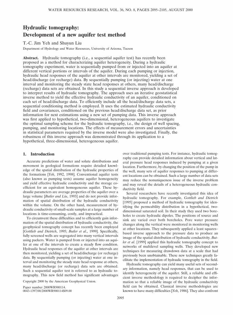
Effects of horizontal well spacing and vertical packer inter-vals are shown in Figures 1a and 1b, where the contour mapsof L1 and L2 for different values of Dx/lx and Dz/lz areplotted. The correlation scales in the x direction and the zdirection are denoted by lx and lz, Dx is the separationdistance between the two wells, and Dz is the vertical distancebetween neighboring packers. The “optimal” horizontal andvertical intervals are defined as those that yield the minimumof L1 and L2 over the entire domain. According to Figures 1aand 1b the optimal distance between the two wells (horizontalinterval) is approximately half of the horizontal correlationscale. This distance cannot be too large or too small becausethe best estimate of conductivity values is near the vicinity ofthe wells where pressure changes are collected (see discussionin section 5). The optimal vertical distance between packersalong the well (vertical interval) should be as small as possible(at least smaller than 0.5 times the vertical correlation scale).Also shown is that the separation distance between the twowells has more influence on the conductivity estimates thanthat between vertical monitoring points along the well.

3.3. Optimal Pumping Interval

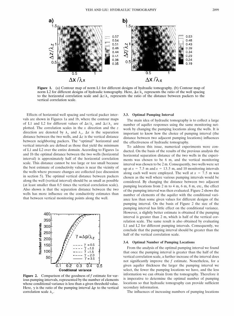
The main idea of hydraulic tomography is to collect a largenumber of aquifer responses using the same monitoring net-work by changing the pumping locations along the wells. It isimportant to know how the choice of pumping interval (thedistance between two adjacent pumping locations) influencesthe effectiveness of hydraulic tomography.

To address this issue, numerical experiments were con-ducted. On the basis of the results of the previous analysis thehorizontal separation distance of the two wells in the experi-ments was chosen to be 6 m, and the vertical monitoringinterval was chosen to be 2 m. Consequently, two wells were setup at x 5 7.5 m and x 5 13.5 m, and 10 monitoring intervalsalong each well were employed. The well at x 5 7.5 m waschosen as the well where various pumping intervals would beconsidered. By changing the distance between two adjacentpumping locations from 2 m to 4 m, 6 m, 8 m, etc., the effectof the pumping interval was then evaluated. Figure 2 shows thenumber of elements of the aquifer with the conditional vari-ance less than some given values for different designs of thepumping interval. On the basis of Figure 2 the size of thepumping interval has little effect on the conditional variance.However, a slightly better estimate is obtained if the pumpinginterval is greater than 2 m, which is half of the vertical cor-relation scale. The same result is also obtained by evaluatingL1 and L2 for different pumping intervals. Consequently, weconclude that the pumping interval should be greater than thehalf of the vertical correlation scale.

3.4. Optimal Number of Pumping Locations

From the analysis of the optimal pumping interval we foundthat once the pumping interval is greater than the half of thevertical correlation scale, a further increase of the interval doesnot significantly improve the f estimate. Nonetheless, for agiven aquifer thickness the larger the pumping interval weselect, the fewer the pumping locations we have, and the lessinformation we can obtain from the tomography. Therefore itis imperative to determine the optimal number of pumpinglocations so that hydraulic tomography can provide sufficientsecondary information.

The influences of increasing numbers of pumping locations

Figure 2. Comparison of the goodness of f estimate for var-ious pumping intervals, represented by the number of elementswhose conditional variance is less than a given threshold value.Here, g is the ratio of the pumping interval Dp to the verticalcorrelation scale lz.

Figure 1. (a) Contour map of norm L1 for different designs of hydraulic tomography. (b) Contour map ofnorm L2 for different designs of hydraulic tomography. Here, Dx/lx represents the ratio of the well spacingto the horizontal correlation scale and Dz/lz represents the ratio of the distance between packers to thevertical correlation scale.


on the effectiveness of the tomography are shown in Figures 3aand 3b. Figure 3a plots the number of f estimates with condi-tional variance lower than the specified threshold value fordifferent numbers of pumping locations. For a given thresholdvalue of the conditional variance (for instance, 0.1), as thenumber of pumping locations increases from 2 to 4, the num-ber of f estimates with conditional variance smaller than 0.1increases from 47 to 147. As the number of pumping locationsincreases to 5, the number of good f estimates increases from147 to 164, showing that the rate of improvement decreases.The same trend is also shown in Figure 3b, where the values ofL1 and L2 decrease significantly when the number of pumpinglocations increases from 2 to 4. Then, the decrease becomesmoderate, and L1 and L2 gradually approach a constant valuewhen five pumping locations are used. The results show that anincrease in the number of pumping locations improves the finalf estimate, but the improvement diminishes as more pumpinglocations are used, indicating that certain data sets generatedfrom hydraulic tomography may provide redundant informa-tion. On the basis of this example the optimal number ofpumping location is five (20 m/4 m; here 20 m is the aquiferdepth, and 4 m is the vertical correlation scale). For a genericaquifer we may conclude that the optimal number of pumpinglocation is the ratio of the aquifer depth to the vertical corre-lation scale.

3.5. Effect of Pumping Rate

Our numerical experiments show that the pumping rate doesnot affect the final estimate of conductivity. Under steady stateflow conditions an increase in the pumping rate leads to anincrease in the hydraulic gradient, which subsequently affectsthe sensitivity of head with respect to saturated conductivity.Such an increase in hydraulic gradients also results in an in-crease in head variance, but the cross correlation between thehead and the conductivity remains the same. Consequently, theincrease in the pumping rate does not affect the cokrigingweights and does not influence the estimate [Li and Yeh, 1998].In other words, different pumping rates will yield identicalresults. One must recognize, though, that in practice, pressure

head data may be corrupted by noises. Thus an increase inpumping rate may increase the signal-to-noise ratio such thatthe inversion of hydraulic tomography data can yield betterresults.

4. Uncertainty AnalysisOur inverse method for the hydraulic tomography requires

the knowledge of mean, variance, and correlation structure ofthe conductivity field, head data sets and the associated pump-ing rates, and some conductivity values if they are available.While head data and pumping rates can be collected during thetomography, several means can be employed to obtain themean, variance, and correlation structure of the conductivity.For example, one can estimate them on the basis of coresamples and well logs if they are available, or one can employthe structure identification approach developed by Kitanidisand Vomvoris [1983]. Geophysical survey is an alternative fordetermining correlation scales [Rea and Knight, 1998], and thetraditional aquifer test analysis assuming aquifer homogeneityis a good way to estimate the mean conductivity.

Nevertheless, these statistical parameters are estimates andnot known precisely, and measurement errors in pressureheads are inevitable. Therefore the influence of the uncer-tainty in the statistical parameters and the effects of measure-ment errors on the estimate by our sequential inverse methodare discussed next.

4.1. Uncertainty in the Mean and Varianceof Hydraulic Conductivity

Without collecting a large number of hydraulic conductivitydata sets the mean and variance estimates involve uncertainty.How the uncertainty affects the estimate of hydraulic conduc-tivity by our inverse method needs to be addressed. Severalnumerical experiments were conducted, and the results showthat the uncertainty in the mean conductivity can cause theshift of the mean of our estimated conductivity field. Thepattern of heterogeneity remains almost the same. On theother hand, the uncertainty associated with the variance of

Figure 3. (a) Comparison of the goodness of f estimate for various numbers of pumping locations, repre-sented by the number of elements whose conditional variance is less than a given threshold value. A, twopumping locations; B, three pumping locations; C, four pumping locations; and D, five pumping locations. (b)Norm L1 and L2 versus number of pumping locations.


conductivity has no influence on the final estimate. This isattributed to the fact that our inverse approach relies on thecorrelation and cross correlation, which do not involve thevariance. Specifically, as the variance term appeared on bothsides of the system of equations (6) and (8), it is factored outand canceled when solving the equations for weights.

4.2. Uncertainty in Correlation Scales

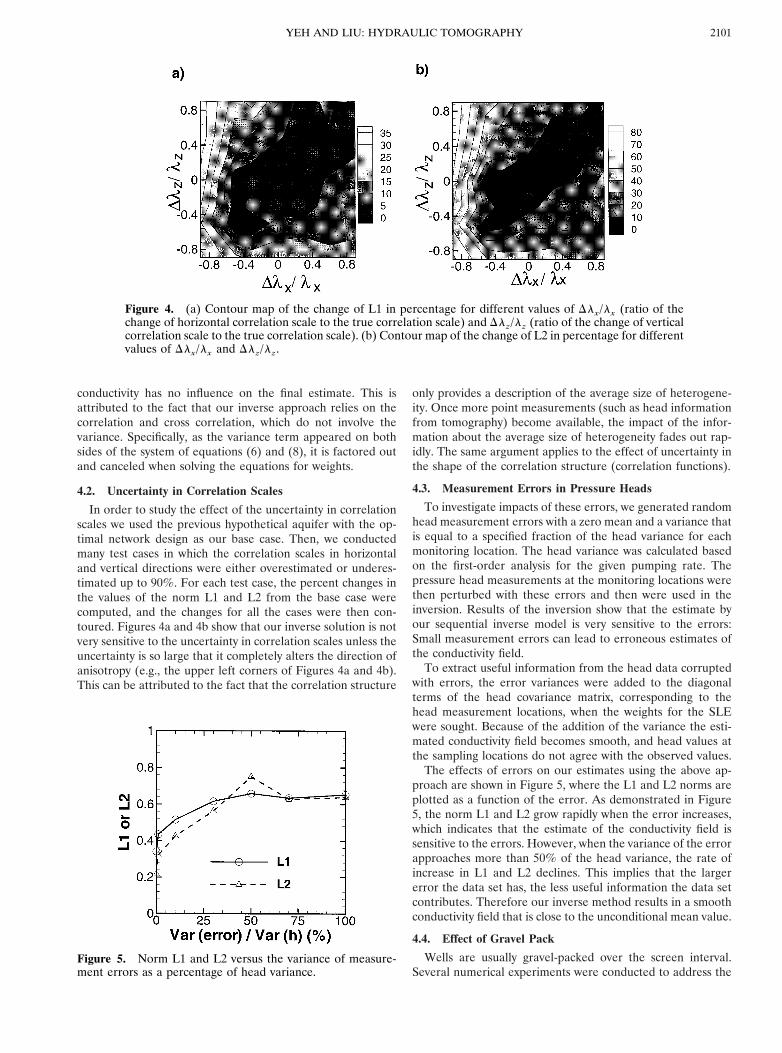
In order to study the effect of the uncertainty in correlationscales we used the previous hypothetical aquifer with the op-timal network design as our base case. Then, we conductedmany test cases in which the correlation scales in horizontaland vertical directions were either overestimated or underes-timated up to 90%. For each test case, the percent changes inthe values of the norm L1 and L2 from the base case werecomputed, and the changes for all the cases were then con-toured. Figures 4a and 4b show that our inverse solution is notvery sensitive to the uncertainty in correlation scales unless theuncertainty is so large that it completely alters the direction ofanisotropy (e.g., the upper left corners of Figures 4a and 4b).This can be attributed to the fact that the correlation structure

only provides a description of the average size of heterogene-ity. Once more point measurements (such as head informationfrom tomography) become available, the impact of the infor-mation about the average size of heterogeneity fades out rap-idly. The same argument applies to the effect of uncertainty inthe shape of the correlation structure (correlation functions).

4.3. Measurement Errors in Pressure Heads

To investigate impacts of these errors, we generated randomhead measurement errors with a zero mean and a variance thatis equal to a specified fraction of the head variance for eachmonitoring location. The head variance was calculated basedon the first-order analysis for the given pumping rate. Thepressure head measurements at the monitoring locations werethen perturbed with these errors and then were used in theinversion. Results of the inversion show that the estimate byour sequential inverse model is very sensitive to the errors:Small measurement errors can lead to erroneous estimates ofthe conductivity field.

To extract useful information from the head data corruptedwith errors, the error variances were added to the diagonalterms of the head covariance matrix, corresponding to thehead measurement locations, when the weights for the SLEwere sought. Because of the addition of the variance the esti-mated conductivity field becomes smooth, and head values atthe sampling locations do not agree with the observed values.

The effects of errors on our estimates using the above ap-proach are shown in Figure 5, where the L1 and L2 norms areplotted as a function of the error. As demonstrated in Figure5, the norm L1 and L2 grow rapidly when the error increases,which indicates that the estimate of the conductivity field issensitive to the errors. However, when the variance of the errorapproaches more than 50% of the head variance, the rate ofincrease in L1 and L2 declines. This implies that the largererror the data set has, the less useful information the data setcontributes. Therefore our inverse method results in a smoothconductivity field that is close to the unconditional mean value.

4.4. Effect of Gravel Pack

Wells are usually gravel-packed over the screen interval.Several numerical experiments were conducted to address the

Figure 5. Norm L1 and L2 versus the variance of measure-ment errors as a percentage of head variance.

Figure 4. (a) Contour map of the change of L1 in percentage for different values of Dlx/lx (ratio of thechange of horizontal correlation scale to the true correlation scale) and Dlz/lz (ratio of the change of verticalcorrelation scale to the true correlation scale). (b) Contour map of the change of L2 in percentage for differentvalues of Dlx/lx and Dlz/lz.


effects of omitting the gravel pack in the inverse modeling. Inthe experiments, gravel packs of different uniform conductivityvalue around the two wells were considered in the forwardsimulation to produce head measurements. The measuredheads were then used in the inversion. Results of the inversionshow that the influence of the gravel pack depends upon thecontrast between the hydraulic conductivity of the backfilledgravel and the mean conductivity of the aquifer system. If theconductivity of the gravel pack is close to the geometric meanof the conductivity of the aquifer, then its effect is negligible.However, if the gravel pack has a conductivity value that isseveral orders of magnitude greater than the geometric meanof the aquifer, then its impact is significant. Since the gravelpack changes the head distribution, the effect can be mini-mized by treating it as the head measurement error.

5. Monte Carlo SimulationsAs mentioned in section 2.2, the conditional covariance

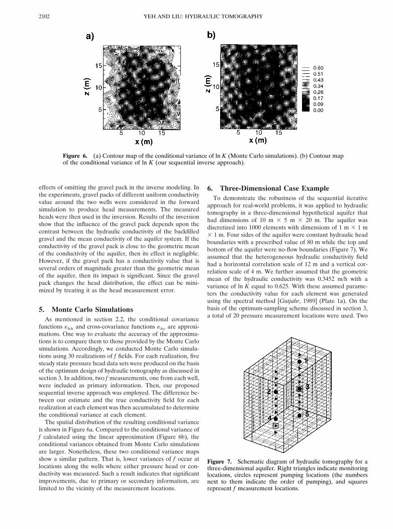
functions «hh and cross-covariance functions «hy are approxi-mations. One way to evaluate the accuracy of the approxima-tions is to compare them to those provided by the Monte Carlosimulations. Accordingly, we conducted Monte Carlo simula-tions using 30 realizations of f fields. For each realization, fivesteady state pressure head data sets were produced on the basisof the optimum design of hydraulic tomography as discussed insection 3. In addition, two f measurements, one from each well,were included as primary information. Then, our proposedsequential inverse approach was employed. The difference be-tween our estimate and the true conductivity field for eachrealization at each element was then accumulated to determinethe conditional variance at each element.

The spatial distribution of the resulting conditional varianceis shown in Figure 6a. Compared to the conditional variance off calculated using the linear approximation (Figure 6b), theconditional variances obtained from Monte Carlo simulationsare larger. Nonetheless, these two conditional variance mapsshow a similar pattern. That is, lower variances of f occur atlocations along the wells where either pressure head or con-ductivity was measured. Such a result indicates that significantimprovements, due to primary or secondary information, arelimited to the vicinity of the measurement locations.

6. Three-Dimensional Case ExampleTo demonstrate the robustness of the sequential iterative

approach for real-world problems, it was applied to hydraulictomography in a three-dimensional hypothetical aquifer thathad dimensions of 10 m 3 5 m 3 20 m. The aquifer wasdiscretized into 1000 elements with dimensions of 1 m 3 1 m3 1 m. Four sides of the aquifer were constant hydraulic headboundaries with a prescribed value of 80 m while the top andbottom of the aquifer were no-flow boundaries (Figure 7). Weassumed that the heterogeneous hydraulic conductivity fieldhad a horizontal correlation scale of 12 m and a vertical cor-relation scale of 4 m. We further assumed that the geometricmean of the hydraulic conductivity was 0.3452 m/h with avariance of ln K equal to 0.625. With these assumed parame-ters the conductivity value for each element was generatedusing the spectral method [Gutjahr, 1989] (Plate 1a). On thebasis of the optimum-sampling scheme discussed in section 3,a total of 20 pressure measurement locations were used. Two

Figure 6. (a) Contour map of the conditional variance of ln K (Monte Carlo simulations). (b) Contour mapof the conditional variance of ln K (our sequential inverse approach).

Figure 7. Schematic diagram of hydraulic tomography for athree-dimensional aquifer. Right triangles indicate monitoringlocations, circles represent pumping locations (the numbersnext to them indicate the order of pumping), and squaresrepresent f measurement locations.


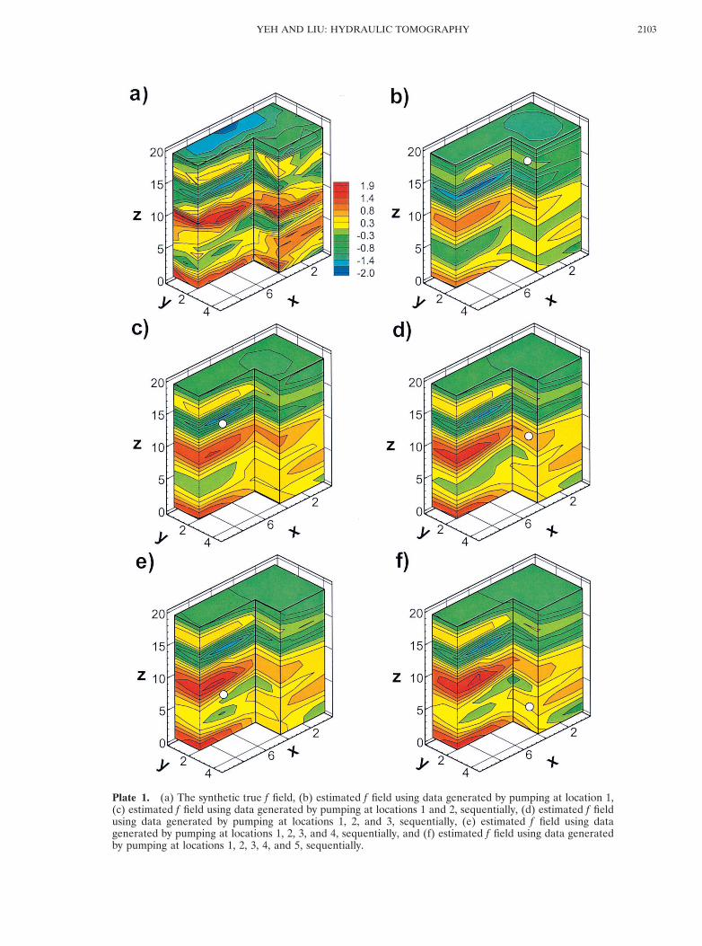
Plate 1. (a) The synthetic true f field, (b) estimated f field using data generated by pumping at location 1,(c) estimated f field using data generated by pumping at locations 1 and 2, sequentially, (d) estimated f fieldusing data generated by pumping at locations 1, 2, and 3, sequentially, (e) estimated f field using datagenerated by pumping at locations 1, 2, 3, and 4, sequentially, and (f) estimated f field using data generatedby pumping at locations 1, 2, 3, 4, and 5, sequentially.


conductivity measurements were taken on each of the wellslocated in the synthetic flow domain (Figure 7). A three-dimensional steady state flow field created by pumping at aselected interval, with a discharge of 20 m3/h, was then simu-lated, and the head responses at other intervals were moni-tored. By sequentially pumping at five different vertical loca-tions (Figure 7), five pressure/discharge data sets wereobtained.

For each set of data the SLE was used to determine theconditional effective hydraulic conductivity field. The field ob-tained from this set of head measurements was used as priorinformation for the next estimation of the conductivity field,using the next set of pressure/discharge data. This procedurewas performed sequentially.

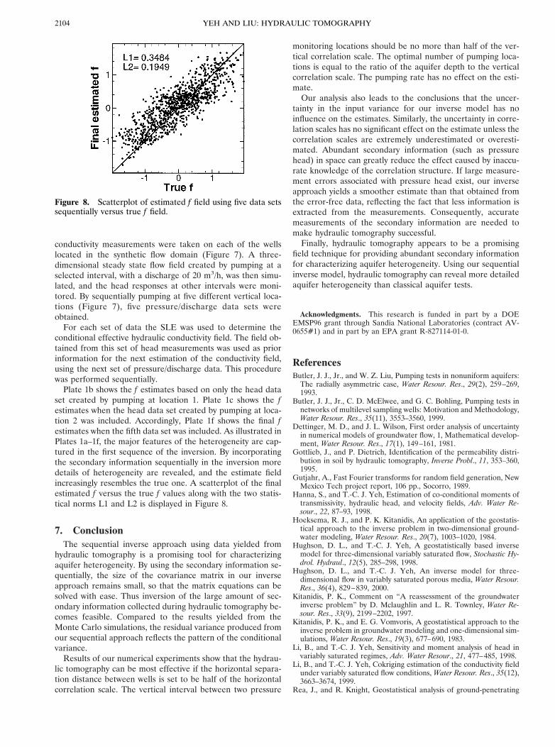
Plate 1b shows the f estimates based on only the head dataset created by pumping at location 1. Plate 1c shows the festimates when the head data set created by pumping at loca-tion 2 was included. Accordingly, Plate 1f shows the final festimates when the fifth data set was included. As illustrated inPlates 1a–1f, the major features of the heterogeneity are cap-tured in the first sequence of the inversion. By incorporatingthe secondary information sequentially in the inversion moredetails of heterogeneity are revealed, and the estimate fieldincreasingly resembles the true one. A scatterplot of the finalestimated f versus the true f values along with the two statis-tical norms L1 and L2 is displayed in Figure 8.

7. ConclusionThe sequential inverse approach using data yielded from

hydraulic tomography is a promising tool for characterizingaquifer heterogeneity. By using the secondary information se-quentially, the size of the covariance matrix in our inverseapproach remains small, so that the matrix equations can besolved with ease. Thus inversion of the large amount of sec-ondary information collected during hydraulic tomography be-comes feasible. Compared to the results yielded from theMonte Carlo simulations, the residual variance produced fromour sequential approach reflects the pattern of the conditionalvariance.

Results of our numerical experiments show that the hydrau-lic tomography can be most effective if the horizontal separa-tion distance between wells is set to be half of the horizontalcorrelation scale. The vertical interval between two pressure

monitoring locations should be no more than half of the ver-tical correlation scale. The optimal number of pumping loca-tions is equal to the ratio of the aquifer depth to the verticalcorrelation scale. The pumping rate has no effect on the esti-mate.

Our analysis also leads to the conclusions that the uncer-tainty in the input variance for our inverse model has noinfluence on the estimates. Similarly, the uncertainty in corre-lation scales has no significant effect on the estimate unless thecorrelation scales are extremely underestimated or overesti-mated. Abundant secondary information (such as pressurehead) in space can greatly reduce the effect caused by inaccu-rate knowledge of the correlation structure. If large measure-ment errors associated with pressure head exist, our inverseapproach yields a smoother estimate than that obtained fromthe error-free data, reflecting the fact that less information isextracted from the measurements. Consequently, accuratemeasurements of the secondary information are needed tomake hydraulic tomography successful.

Finally, hydraulic tomography appears to be a promisingfield technique for providing abundant secondary informationfor characterizing aquifer heterogeneity. Using our sequentialinverse model, hydraulic tomography can reveal more detailedaquifer heterogeneity than classical aquifer tests.

Acknowledgments. This research is funded in part by a DOEEMSP96 grant through Sandia National Laboratories (contract AV-0655#1) and in part by an EPA grant R-827114-01-0.

ReferencesButler, J. J., Jr., and W. Z. Liu, Pumping tests in nonuniform aquifers:

The radially asymmetric case, Water Resour. Res., 29(2), 259–269,1993.

Butler, J. J., Jr., C. D. McElwee, and G. C. Bohling, Pumping tests innetworks of multilevel sampling wells: Motivation and Methodology,Water Resour. Res., 35(11), 3553–3560, 1999.

Dettinger, M. D., and J. L. Wilson, First order analysis of uncertaintyin numerical models of groundwater flow, 1, Mathematical develop-ment, Water Resour. Res., 17(1), 149–161, 1981.

Gottlieb, J., and P. Dietrich, Identification of the permeability distri-bution in soil by hydraulic tomography, Inverse Probl., 11, 353–360,1995.

Gutjahr, A., Fast Fourier transforms for random field generation, NewMexico Tech project report, 106 pp., Socorro, 1989.

Hanna, S., and T.-C. J. Yeh, Estimation of co-conditional moments oftransmissivity, hydraulic head, and velocity fields, Adv. Water Re-sour., 22, 87–93, 1998.

Hoeksema, R. J., and P. K. Kitanidis, An application of the geostatis-tical approach to the inverse problem in two-dimensional ground-water modeling, Water Resour. Res., 20(7), 1003–1020, 1984.

Hughson, D. L., and T.-C. J. Yeh, A geostatistically based inversemodel for three-dimensional variably saturated flow, Stochastic Hy-drol. Hydraul., 12(5), 285–298, 1998.

Hughson, D. L., and T.-C. J. Yeh, An inverse model for three-dimensional flow in variably saturated porous media, Water Resour.Res., 36(4), 829–839, 2000.

Kitanidis, P. K., Comment on “A reassessment of the groundwaterinverse problem” by D. Mclaughlin and L. R. Townley, Water Re-sour. Res., 33(9), 2199–2202, 1997.

Kitanidis, P. K., and E. G. Vomvoris, A geostatistical approach to theinverse problem in groundwater modeling and one-dimensional sim-ulations, Water Resour. Res., 19(3), 677–690, 1983.

Li, B., and T.-C. J. Yeh, Sensitivity and moment analysis of head invariably saturated regimes, Adv. Water Resour., 21, 477–485, 1998.

Li, B., and T.-C. J. Yeh, Cokriging estimation of the conductivity fieldunder variably saturated flow conditions, Water Resour. Res., 35(12),3663–3674, 1999.

Rea, J., and R. Knight, Geostatistical analysis of ground-penetrating

Figure 8. Scatterplot of estimated f field using five data setssequentially versus true f field.


radar data: A means of describing spatial variation in the subsurface,Water Resour. Res., 34(3), 329–339, 1998.

Sun, N.-Z., and W. W.-G. Yeh, A stochastic inverse solution for tran-sient groundwater flow: Parameter identification and reliability anal-ysis, Water Resour. Res., 28(12), 3269–3280, 1992.

Sykes, J.-F., J. L. Wilson, and R. W. Andrews, Sensitivity analysis ofsteady state groundwater flow using adjoint operators, Water Resour.Res., 21(3), 359–371, 1985.

van Genuchten, M. T., A closed-form equation for predicting thehydraulic conductivity of unsaturated soils, Soil Sci. Soc. Am. J., 44,892–898, 1980.

Vargas-Guzman, A. J., and T.-C. J. Yeh, Sequential kriging andcokring: Two powerful geostatistical approaches, Stochastic Environ.Res. Risk Assess., 13, 416–435, 1999.

Yeh, T.-C. J., Stochastic modeling of groundwater flow and solutetransport in aquifers, J. Hydrol. Processes, 6, 369–395, 1992.

Yeh, T.-C. J., Scale issues of heterogeneity in vadose-zone hydrology,in Scale Dependence and Scale Invariance in Hydrology, edited by G.Sposito, Cambridge Univ. Press, New York, 1998.

Yeh, T.-C. J., A. L. Gutjahr, and M. Jin, An iterative cokriging-like

technique for groundwater flow modeling, Ground Water, 33(1),33–41, 1995.

Yeh, T.-C., M. Jin, and S. Hanna, An iterative stochastic inversemethod: Conditional effective transmissivity and hydraulic headfields, Water Resour. Res., 32(1), 85–92, 1996.

Yeh, W. W-G., Review of parameter identification procedures ingroundwater hydrology: The inverse problem, Water Resour. Res.,22(1), 95–108, 1986.

Zhang, J., and T.-C. J. Yeh, An iterative geostatistical inverse methodfor steady flow in the vadose zone, Water Resour. Res., 33(1), 63–71,1997.

S. Liu and T.-C. J. Yeh, Department of Hydrology and Water Re-sources, University of Arizona, John W. Harshbarger Building, P. O.Box 210011, Tucson, AZ 85721-0011. ([email protected])

(Received October 12, 1999; revised April 18, 2000;accepted April 18, 2000.)


hydraulic tomography: development of a new...

Documents