Applied Mathematics, 2016, 7, 2336-2353 http://www.scirp.org/journal/am

ISSN Online: 2152-7393 ISSN Print: 2152-7385

DOI: 10.4236/am.2016.718184 December 19, 2016

Hydraulic Reliability Assessment and Optimal Rehabilitation/Upgrading Schedule for Water Distribution Systems

Wei Peng, Rene V. Mayorga

Faculty of Engineering, University of Regina, Regina, Canada

Abstract This paper develops an innovative approach to optimize a long-term rehabilitation and upgrading schedule (RUS) for a water distribution system with considering both hydraulic failure and mechanical performance failure circumstances. The proposed approach assesses hydraulic reliability dynamically and then optimizes the long-term RUS in sequence for a water distribution system. The uncertain hydraulic parameters are treated as random numbers in a stochastic hydraulic reliability assessment. The methodologies used for optimization in a stochastic environment are: Monte Carlo Simulation, EPANET Simulation, Genetic Algorithms, Shamir and Howard’s Expo-nential Model, Threshold Break Rate Model and Two-Stage Optimization Model. The proposed approach is conducted on a simulation model of water distribution network in a computer by two universal codes, namely the hydraulic reliability code and the optimal RUS code. The applicability of this approach is verified in an exam-ple of a benchmark water distribution network.

Keywords Optimization, Stochastic, Water Distribution, Rehabilitation, Upgrade, Hydraulic Reliability

1. Introduction

Water distribution systems (WDSs) require huge investments in their construction and maintenance. For this reason, it is an important need to improve their efficiency by ways of minimizing their costs and maximizing the benefits. In the last several decades, a significant number of optimization methods have been developed using linear pro-gramming, dynamic programming, enumeration techniques, heuristic methods, and

How to cite this paper: Peng, W. and Ma- yorga, R.V. (2016) Hydraulic Reliability As- sessment and Optimal Rehabilitation/Up- grading Schedule for Water Distribution Sys- tems. Applied Mathematics, 7, 2336-2353. http://dx.doi.org/10.4236/am.2016.718184 Received: September 20, 2016 Accepted: December 16, 2016 Published: December 19, 2016 Copyright © 2016 by authors and Scientific Research Publishing Inc. This work is licensed under the Creative Commons Attribution International License (CC BY 4.0). http://creativecommons.org/licenses/by/4.0/

Open Access

W. Peng, R. V. Mayorga

2337

evolutionary techniques [1]. However, water distribution systems are so complex that most of the researches only address partial issues. For example, the previous optimal maintenance schedule studies focused on either hydraulic capacity or mechanical per-formance failure by minimizing costs rather than the combination of them. The pro-posed study will develop such an innovative tool that considers the deterioration over time of both structural integrity and hydraulic capacity of every pipe, and optimizes the Rehabilitation & Upgrading Schedule (RUS) for an entire WDS.

Hydraulic reliability assessment is used to study the deterioration over time of struc-tural integrity and hydraulic capacity of WDSs; in other words, it is to study the me-chanical failure and hydraulic failure over time. However, there are no universally ac-cepted definitions for hydraulic reliability [2]. Here, we define hydraulic reliability as “the ability of a distribution system to meet the demands that are placed on it, where demands are specified in terms of: (i) the flow to be supplied, and (ii) the range of pressure at which these flow rates must be provided [3].” Hydraulic failures occur when the demand nodes do not receive sufficient flow and/or adequate pressure, due to old pipes with low roughness arising from corrosion and deposition, increases of demand and pressure head requirements, inadequate pipe sizes, insufficient pumping or/and storage capabilities, etc. In addition, due to the fact that the demand is spatially and temporally distributed, hydraulic failures at critical locations in the distribution system may be more important than the average system reliability [4]. Mechanical failures in-volve pipe breakage, pump failure, power outages, control valve failure, etc. Mechanical failure of the infrastructure components is also integrally linked with hydraulic failure. For instance, pipe breakage is a mechanical failure, and the occurrence of a pipe break will eventually result in insufficient flow rate and/or inadequate pressure head on the demand nodes.

In the previous researches, two methodologies were developed to compute the hy-draulic reliability. One is the Monte-Carlo simulation (MCS) technique, which can bring more accurate reliability estimation [5] [6], but requires a large number of trials to ensure accuracy thereby resulting in a computationally inefficient problem. Another is a linear probabilistic hydraulic model, called the first-order reliability method [7] [8], which can overcome the computationally inefficient problem in MCS, but has a lower accuracy. Due to the rapid development of computer technology, the MCS has demon-strated its superiority in the hydraulic reliability computation. In this paper, the MCS is chosen to calculate the probabilistic problem of hydraulic reliability. A free simulation software EPANET [9] is incorporated with this MCS to evaluate the nodal & system re-liability of a water distribution system. It’s worth noting that the hydraulic reliability assessment here only refers to the hydraulic failure measurement but the mechanical failure measurement.

The RUS optimization model is based on its hydraulic reliability assessment. It is subdivided into two stages. The first stage is the planning of upgrading and paralleling pipes due to hydraulic failure potential (such as demand and pressure); the second stage is the schedule of repairing and replacing pipes due to mechanical failure poten-

W. Peng, R. V. Mayorga

2338

tial (such as pipe breakage, pump, or aging of pipe). The first stage is domination due to hydraulic failures that directly result in insufficient flow and/or inadequate pressure. On the other hand, mechanical failures only indirectly influence water supply on the demand nodes. For example, the occurrence of one pipe break of a paralleling pipe sys-tem may only slightly lower the water flow rate and/or water pressure, but water supply may still be sufficient.

Previously, many research papers used various methodologies to study the optimal maintenance schedule to the pipe networks focusing on either the hydraulic capacity or the mechanical performance failure. Some of the earlier studies used linear program-ming [10] while the later studies utilized nonlinear programming [8] [11] to study the hydraulic failure for the optimal planning. Many of the recent literature applied genetic algorithms for the determination of the lowest repairing or replacing costs [12] [13]. Some researches had shown several advantages over more traditional optimization me-thods [14] [15] [16]. In the mechanical failure area, Shamir and Howard applied regres-sion analysis to obtain a relationship for the breakage rate of a pipe as a function of time [17]. Deb et al. suggested a failure probabilistic model to estimate miles of pipes to be replaced on an annual basis [18]. Ascher and Feingold gave a threshold break rate function by using a statistical reliability model [19].

This paper is to develop such innovative approach, with considers both hydraulic failure and mechanical performance failure, to dynamically assess hydraulic reliability and then continue to find a best option for the long-term RUS of a water distribution system. This approach is conducted on a simulation model of water distribution net-work in a computer by two universal codes, namely the hydraulic reliability code and the optimal RUS code, and it eventually will be applied in the real water distribution networks planning. The applicability of this approach is verified in an example of a benchmark water distribution network.

2. Methodology 2.1. Hydraulic Reliability Assessment

Hydraulic failures occur when the demand nodes do not receive sufficient flow and/or adequate pressure, due to old pipes with low roughness arising from corrosion and de-position, increases of demand and pressure head requirements, inadequate pipe sizes, insufficient pumping or/and storage capabilities, etc. Mechanical failures involve pipe breakage, pump failure, power outages, control valve failure, etc. Mechanical failure of the infrastructure components is also integrally linked with hydraulic failure. For in-stance, pipe breakage is a mechanical failure, and the occurrence of a pipe break will eventually result in insufficient flow rate and/or inadequate pressure head on the de-mand nodes. Mathematically, the system hydraulic reliability equals 1 minus the system failure which shown in Figure 1. It notes that there has not a measurement method to directly identify whether a failure is hydraulic or mechanical.

2.1.1. Nodal Hydraulic Failure Probability Hydraulic failure at a given node occurs when the supplied flow or pressure is less than

W. Peng, R. V. Mayorga

2339

System Failure =1- System Hydraulic Reliability

Hydraulic Failure Mechanical Failure

Demand Increase

Pipe Breakage

Electrical Components

Failure

Inadequate Pipe Size

Insufficient Pump/Storage Capabilities

Corrosion and

Deposition

Others Others

Figure 1. Flowchart of system failure.

the required minimum flow or the required minimum pressure at that node. Consider-ing we will use EPANET for simulation that the hydraulic simulator always satisfies water demand (because of applying the nodal mass balance equation) but not pressure head, this approach automatically assumes that water demand is satisfied. The nodal mass balance equation can be expressed as:

( ) 0 1,2, ,i ij i jj

D f H H i N∈Ω

+ − = =∑ (1)

where Di is demand at node i; Hi is head at node i; Hj is head at node j; N is total num-ber of the demand nodes with unknown heads; Ω is set of nodes connected directly to node i; ( )*ijf is a nonlinear function relating the hydraulic loss and flow rate in the pipe connecting node i to node j. The nonlinear function used here is the Hazen- Williams or the Colebrook-White equation.

In the above equation, nodal pressure head is an unknown decision variable, and water demands are state variables. This equation can be expressed in a more compact form:

( ), 0 1,2, ,i i iF H X i N= = (2)

where Fi(*) is a vector of functions representing the mass balance at each node; Hi is a vector of supplied pressure heads at each node; ( )T

1 2, , ,i k iX x x x= is a vector of state

variables and k is the total number of variables. In the study of the hydraulic perfor-mance failure, we define water demands Di, pipe coefficients Ci, and tank/storage levels Li as known state variables. Thus, the vector of state variables in this study can be ex-pressed as ( )T, ,i i i iX D C L= ; T represents the matrix transpose operation. Moreover,

W. Peng, R. V. Mayorga

2340

due to uncertainty, those known state variables will be treated as random values. Each random variable is expressed as a probability distribution, and then a random number generator is used to generate the values of Di for each node, the values of Ci for each pipe, and the values of Li for each tank/storage. Incorporation with EPANET, Monte Carlo simulation (MCS) technique can be applied to produce the random values of pressure head.

EPANET: EPANET is free public domain software developed by USEPA. It performs extended period simulation of hydraulic behavior within pressurized pipe networks [9]. A network consists of pipes, nodes, pumps, valves and storage tanks or reservoirs. EPANET tracks the flow water in each pipe, the pressure at each node, the level of wa-ter in each tank during a simulation period. Running under Windows, EPANET pro-vides an integrated environment for editing network input data, running hydraulic and water quality simulations, and viewing the results in a variety of formats. In this study, water demands, pipe coefficients, tank/storage levels are inputting data during the si-mulation; pressure heads are outputs. We assume that pumps and valves are in good operation condition. The failure of pumps and valves is considered in the area of me-chanical failure.

Monte Carlo Simulation: Monte Carlo simulation involves repeated generation of pseudovalues for the modeling inputs, drawn from known probability distributions within the ranges of possible values. In this study, this process will be completed by computer, where three random variables (water demand Di, pipe coefficients Ci, and tank/storage level Li) are produced synchronously at each time. The generated pseudo-values are then used as inputs for EPANET model to produce the supplied pressure head values of Hi. The Monte Carlo simulation implementation in a node i includes steps: (1) development of the representative probability distribution functions for se-lected model input parameters; (2) generation of pseudovalues for each of the selected input parameters from the distribution developed in the previous step; (3) implementa-tion of EPANET model with the pseudovalues to generate a pressure head value of Hi; (4) comparison of the calculated value of Hi with the minimum allowable head L

iH ; (5) repeated application of the previous two steps; (6) presentation of the results, and analysis of the results for decision making.

In the above step (4) of the MCS procedure, we defined LiH as the minimum al-

lowable head at a demand node. Thus, the probability of hydraulic performance failure at a demand node can be expressed as

( ) ( )0

dLiHH L S D

i i i i i i iP P H H D D f H H= < = = ∫ (3)

where ( )if H is the probability density function of the supplied pressure head; DiS is

the supplied flow rate at the node i, and DiD is the water demand at the node i.

2.1.2. Mechanical Failure Probability Mechanical failure involves pipe breakages and electric component failures (such as pump failure, power outages, control valve failure, etc). There are many factors that may cause pipe breaks, for instance, aging, physical bending stress, chemical and bio-

W. Peng, R. V. Mayorga

2341

logical corrosion, etc. Among these factors, aging, material type, dimension, and bed-ding quality are important factors in predicting pipe breakage. Here we demonstrate two exponential break rate equations. Shamir and Howard’s exponential break rate model describes an exponential relationship between aging and breakage [17].

( ) ( ) ( )00 e 1, 2, ,j jA t tpp

j jP t P t j M

−= = (4)

where Aj is the growth rate coefficient of the pipe j; ( ) pjP t is the number of breaks per

1000 ft. length of pipe j in year t; t is time in years; t0 is base year for the analysis (pipe installation year, or the first year for which data are available); M is total number of pipes.

In real situation, a primary cause of unreliability is the removal of water lines or pumps from service primarily due to breaks or power outages. A probability of an elec-tromechanical component E

kP (k = 1, 2, …, U; where U is total number of electric components), such as a pump or a valve, being out of service can be included as anoth-er random variable that supported by historical data.

2.1.3. System Hydraulic Reliability Assessment (See Figure 2) Different water demand has different importance. For example, a hospital water de-mand has the highest importance, and the water demand of a park area may have a lower importance. We weight failure probabilities to reflect their different importance

Figure 2. Procedure of system hydraulic reliability assessment.

W. Peng, R. V. Mayorga

2342

impacts. Then, the system failure probability SP can be defined as the maximum in-dividual failure probability in the system

( )Max , , ,H P E F FS i i j j k kP W P W P W P W PΧ= (5)

where , , , Fi j kW W W W are weighting coefficients; H

iP is the probability of hydraulic performance failure at the node i; P

jP is the failure probability of pipe j; EkP is the

failure probability of electromechanical component k; FP is the fire flow failure probability.

The system hydraulic reliability SR is given by

1 .S SR P= − (6)

2.2. Optimal Rehabilitation & Upgrading Schedule

The long term planning of WDSs is an important issue for municipal agents. These agents pay special attention to improve the efficiency of their planning by the ways of minimizing the costs and maximizing the benefits. However, water distribution systems are so complex that most of the researches only address partial issues. For example, the previous optimal maintenance schedule studies only focused on either hydraulic failure or mechanical failure by minimizing costs but the combination of them. This study will develop such an innovative model that considering the deterioration over time of both structural integrity and hydraulic capacity of every pipe, and optimizing the RUS for a whole WDS.

The model identifies the network maintenance into the rehabilitation and the up-grading. It is subdivided into two stages (see Figure 3). The first stage is the planning of

Figure 3. Flowchart of two-stage method.

W. Peng, R. V. Mayorga

2343

upgrading and paralleling pipes due to hydraulic failure potential (such as demand and pressure); the second stage is the schedule of repairing and replacing pipes due to me-chanical failure potential (such as pipe breakage, pump, or aging of pipe). The first stage is domination due to hydraulic failures that directly result in insufficient flow and/or inadequate pressure. On the other hand, mechanical failures only indirectly in-fluence water supply on the demand nodes. For example, the occurrence of one pipe break of a paralleling pipe system may only slightly lower the water flow rate and/or water pressure, but water supply may still be sufficient.

It’s worth noting that we use “potential” to describe hydraulic failures and mechani-cal failures because we refer to those failures in future. Both prediction models of hy-draulic failure and mechanical failure are based on the hydraulic reliability assessment. The hydraulic failure probability is assessed by the Monte Carlo Simulation, and the pipe breakage probability is computed by the Shamir and Howard’s exponential break rate model (shown in Equation (4)). Because mechanical failure probability is obtained in terms of historical data, the optimal upgrading results will not affect the pipe brea-kage probabilities except for the pipes that had been upgraded in the first stage.

2.2.1. Rehabilitation Optimization Model Although the pipe repair cost is much lower than the replacement fee, frequent breaks will result in the cumulative repair expense exceeding the replacement cost. Therefore, we need a methodology to find the critical (or threshold) break rate to determine the timing of repair or replacement [19].

If we assume that the pipe will be replaced at the time of the nth break (it also implies that for the previous (n − 1) breaks only repairs have been performed), we can write the present worth of the total cost of the pipe as

( ) ( )1 1 1i n

ni n

n t ti

C FT

β β=

= ++ +

∑ (7)

where β is the discount rate; it is the time of the ith break measured from the instal-lation year; iC is the repair cost of the ith break; nF is the replacement cost at time

nt ; nT is the present worth. For the total cost nT at time nt to be a minimum, it must satisfy the condition

1 1.n n nT T T− +> < (8)

However, the critical check is to determine the first instance when the condition

1n nT T+ > holds true. Solving for ( )1n nt t+ − , we have

( )

1 1

1

In.

In 1

n n

n nn n

C FF F

t tβ

+ +

+

+

− <+

(9)

Recognizing 1n nt t+ − is the time between the nth and (n + 1)th breaks or time inter-val for the occurrence of one break, we obtain the threshold break rate, Brkth, as the in-verse of nt∆ (where 1n n nt t t+∆ = − ). The threshold break rate is defined as the break rate between subsequent breaks.

W. Peng, R. V. Mayorga

2344

( )th

1 1 1

In 11 1BrkInn n n n n

n n

t t t C FF F

β

+ + +

+= = >∆ −

+

(10)

Now, from the observed data for any given pipe we can derive a current break rate. Whenever the current break rate is equal to or more than Brkth, the pipe should be re-placed. It is worth noting that the optimal rehabilitation schedule information will be transferred to the upgrading optimization process (shown in Figure 4).

2.2.2. Upgrading Optimization Model The hydraulic reliability can indicate the hydraulic performance information for each demand node. If the hydraulic failure probability on a node is lower than the allowable probability, the water provider should replace the inlet pipe with a larger diameter pipe or build a paralleling pipe. Then, the next few questions for the decision maker are: 1). Replace the existing pipeline by a bigger diameter pipeline or build a paralleling pipe-line? 2) What size of pipe should be applied in this replacement or paralleling? 3) The duration of the new inlet pipe that can transfer sufficient water?

The design of water distribution systems is often viewed as a least-cost optimization problem in the previous literatures. The pipe diameters were considered as decision va-riables. Obviously other parameters should be considered as objectives in the optimiza-tion process, such as reliability, redundancy and water quality [20]. However, problems with quantifying these objectives for use within optimization design models kept re-searchers concentrating on the single, least-cost objective. Therefore, the overall objec-tive in the upgrading optimization in this paper is to minimize the total cost. The fol-lowing formulation describes this objective:

Figure 4. Example of distribution system.

W. Peng, R. V. Mayorga

2345

( )Minimize ,m

j j jj

f C R L= ∑ (11)

where ( ),j j jC R L is the cost of pipe j with diameter Rj and length Lj; m is the number of pipes that must be upgraded. The objective is subject to the following constraints:

( ), 0G H D = (12)

L UH H H≤ ≤ (13) L UD D D≤ ≤ (14)

( ) ( ) ( ), , ,L UW H D W H D W H D≤ ≤ (15)

where Equation (12) refers to conservation of flow constraints and energy equations (loop equations); Equation (13) is head boundary constraints; Equation (14) is designed water demand boundary constraints; Equation (15) represents general constraints in-cluding financial constraints.

The decision on either replacement or paralleling pipeline is depended on cost, geo-graphical situation, and the existing pipe condition. Some pipeline geographical condi-tions are not suitable for the laying of parallel pipelines that the only choice is to replace the existing pipelines by larger diameter pipes. However, the geographical condition consideration of the pipe replacement planning is out of the scope of this study. In ad-dition, we have to consider the duration of the upgraded pipeline. If one pipe needed upgrade because low hydraulic capability, simultaneously it was aging pipe that would be replaced in the next few years, it was better to directly be replaced by a new large diameter pipe rather than to build a parallel pipeline.

We assume the length of the term is l, the objective formulation is modified as fol-lows

( ) ( ) 1

1 1Minimize , 1

m l kjk j j

j kf C R L β −

= =

= +∑∑ (16)

where l is the length of the planning period; and k (k = 1, 2, … l) is the year index of pipeline upgrading. The total cost includes the following components:

( ), 1 2jk j jC R L f f= + (17)

1f represents the pipeline costs including installation, paralleling, replacement and repair costs; 2f is the cost of setting up the construction plant and machinery.

2.2.3. Optimization Procedure Pipe Roughness and Water Demand: The pipe roughness and the water demand are two model input parameters that vary over time. The pipe roughness increases over time at a rate that varies according to the pipe type, water quality, and operation and maintenance practices. To model the effect of aging on the carrying capacity of pipes, the equation of Sharp and Walsli [21] was used

( ) ( )age18.0 37.2 log oe a

C tR

+ = −

(18)

W. Peng, R. V. Mayorga

2346

where C(t) is the Hazen-Williams coefficient in year t; eo is the roughness at the time of installation (mm); a is the roughness growth rate (mm/year); and R is the pipe diameter (mm).

The function developed by Dandy et al. [22] is used to predict nodal water demand. PREL

00

DGR1100

tt

i iP

D DP

= +

(19)

where D0j is the base year water demand for the node j and DGR is the annual percen-tage rate of increase in the base demand. DGR was assumed to follow demographic data patterns closely, and so it was taken as the population growth rate with typical values of about 2 to 5; t is the time in years; Pt and P0 are the price per unit volume of water for year t and the base year, respectively; PREL is the price elasticity of demand. A typical range of PREL values is −0.2 to −0.5. Generally it is advisable to increase the price of water in the last 1 or 2 years of the design period for the best results in order to delay the need to upgrade the network. When there is adequate capacity after upgrading, prices can be reduced in order to utilize the system capacity as fully as possible and to maximize economic efficiency. Other demand management options could be used, and self-evidently, the joint effect of all the demand management techniques deployed should be considered.

Genetic Algorithms: We have chosen the genetic algorithms (GA) as the optimiza-tion method. GA is a search technique used in computing to find exact or approximate solutions to optimization and search problems. It is based on the mechanics of natural selection and natural genetics that using biological techniques including inheritance, mutation, selection, and crossover [23]. GA provides a robust and efficient way to search complex parameter spaces for ever better solutions to an optimization problem [23]. Although there are no guarantees that a GA will actually attain the optimum, it generally finds one or more extremely good solutions with relatively little computa-tional effort.

The GA code can also be written by MATLAB. Moreover, EPANET simulation will be run during the GA optimization process. The following steps give the details of the optimization procedure for a repair schedule.

Step 1. Use Equation (4) to calculate each pipeline’s break rate B(i, j); and use Equa-tion (10) to compute each pipeline’s Brkth and then obtain the corresponding replace-ment year Yr(j), where i represents the time of year, and j is the pipe index.

Step 2. Set i = 0; Step 3. i = i + 1; Step 4. Run the hydraulic reliability model and calculate nodal hydraulic reliability

R(i, j) for all studied nodes in a WDS in the ith year; Step 5. Compare the predicted hydraulic reliability with the minimum allowable hy-

draulic reliability Rm(i, j) at the ith year, to find the pipes to be upgraded P(i, j); Step 6. If the replacement year Yr(j) of the upgraded pipe is equal to or more than the

planning term N, then, no paralleling is considered;

W. Peng, R. V. Mayorga

2347

Step 7. Run Optimization Code (GA) to find optimal diameter pipe P(i, j, m) (where m is the index of pipe diameter, both replacement and paralleling use this diameter in-dex), with the objective of minimizing total cost, and subject to the constraint that the R(i, j) should be greater than the maximum of Rm(i, j) during the whole planning pe-riod N. The computation of R(i, j), of course, needs to run the hydraulic reliability pre-diction model;

Step 8. If i < N, then go to step 3; Step 9. Calculate the total cost and record the optimal rehabilitation and upgrading

schedule.

3. Example Application

Figure 4 shows a benchmark hypothetical water distribution system [24] that consists of 16 pipes, 10 demand nodes, two tanks and one reservoir. Tables 1-4 demonstrate the information of system components.

Due to we use the MCS to compute the nodal and system reliability, the iterative process of random number generation of D, C, and L, and hydraulic simulation must be repeated a large number of times. According to the previous studies [6] [8], the op-timal number of iterations is between 500 times to 3000 times. Because the results had tiny different after 2000 iterations, we use 2000 iterations in this study.

There are several probability distributions can achieve random number generation of D, C, and L, such as normal, log-normal, uniform, Pearson and Weibull distributions. According to the literature, normal distribution is the most popular probability distri-bution that used in hydraulic studies [13] [14] [25] [26]. We also use normal distribu-tion for random number generation of D, C, and L.

The Shamir and Howard’s exponential break rate model (shown in Equation (4)) is used to compute the pipe breakage probability. The expected number of failures per year per unit length of pipe Aj is uniformly assumed to be 0.122. The mean values of

Table 1. Node information.

Node No. Elevation (ft) Mean demand (gpm) Min Allowable head (ft)

Res 320 N/A N/A

N1 390 120 50

N2 420 75 50

N3 425 35 50

N4 430 50 50

N5 450 70 50

N6 445 155 50

N7 420 65 50

N8 415 150 50

N9 420 55 50

N10 420 20 50

W. Peng, R. V. Mayorga

2348

Table 2. Pipe information.

Pipe No. Length (ft) Diameter (in) Mean Hazen-Williams Coefficient Aj

P1 890 10 115 0.122

P2 1250 6 110 0.122

P3 835 6 110 0.122

P4 1330 8 110 0.122

P5 1010 6 110 0.122

P6 550 8 130 0.122

P7 425 8 130 0.122

P8 990 8 125 0.122

P9 2100 8 105 0.122

P10 745 8 110 0.122

P11 1100 10 115 0.122

P12 560 6 110 0.122

P13 825 10 115 0.122

P14 500 6 120 0.122

P15 690 6 120 0.122

P16 450 6 120 0.122

Table 3. Tank information.

Tank 1 Tank 2

Base Elevation (ft) 0 0

Min Elevation (ft) 525 535

Initial Elevation (ft) 545 550

Max Elevation (ft) 565 570

Tank Diameter (ft) 35.7 49.3

normal distribution of D, C, and L are obtained from Table 1 to Table 4. The coeffi-cients of variation for D and L are assumed to be 0.2. According to the conclusion of Bao and Mays [6] that system reliability is somewhat insensitive to the type of probabil-ity distribution of pipe roughness when the coefficient of variation C is less than 0.4, we assume the coefficient of variation C is 0.4.

The results of the nodal hydraulic performance failure probability, the pipe breakage probability, and the system hydraulic reliability are shown in Table 5. From the results, we found i). The system reliability shows a great improvement when a reasonable weighing factor is used. ii). The system reliability is 0.892, representing a sample distri-bution of an unsafe system (safe system reliability should be greater than 0.999). iii). the nodal hydraulic performance failure probability is almost one order of magnitude lower than the pipe breakage probability.

W. Peng, R. V. Mayorga

2349

Table 4. Weighting coefficient.

Pipe No. Weighting Coefficient Node No. Weighting Coefficient

P1 1 N1 0.9

P2 0.8 N2 0.8

P3 0.5 N3 0.5

P4 0.5 N4 0.6

P5 0.6 N5 0.5

P6 0.6 N6 0.4

P7 0.6 N7 0.7

P8 0.8 N8 1

P9 0.5 N9 0.9

P10 0.5 N10 0.8

P11 0.7

P12 0.7

P13 0.7

P14 0.9

P15 0.8

P16 0.8

Table 5. Results of reliability assessment.

Pipe No.

Weighting Coefficient

Pipe Failure Prob.

Weighted Pipe fail.

Prob.

Node No.

Weighting Coefficient

Nodal Failure Prob.

Weighted Nodal fail.

Prob.

P1 1 0.098 0.098 N1 0.9 0.0448 0.0403

P2 0.8 0.134 0.107 N2 0.8 0.0016 0.0013

P3 0.5 0.092 0.046 N3 0.5 0.0634 0.0317

P4 0.5 0.142 0.071 N4 0.6 0.0240 0.0144

P5 0.6 0.110 0.066 N5 0.5 0.0408 0.0204

P6 0.6 0.062 0.037 N6 0.4 0.0170 0.0068

P7 0.6 0.048 0.029 N7 0.7 0.0772 0.0540

P8 0.8 0.108 0.082 N8 1 0.0018 0.0018

P9 0.5 0.215 0.108 N9 0.9 0.0810 0.0729

P10 0.5 0.082 0.041 N10 0.8 0.0534 0.0427

P11 0.7 0.119 0.083

P12 0.7 0.063 0.044

P13 0.7 0.091 0.063

P14 0.9 0.056 0.05

P15 0.8 0.077 0.062

P16 0.8 0.051 0.041

System failure probability 0.108

System reliability 0.892

W. Peng, R. V. Mayorga

2350

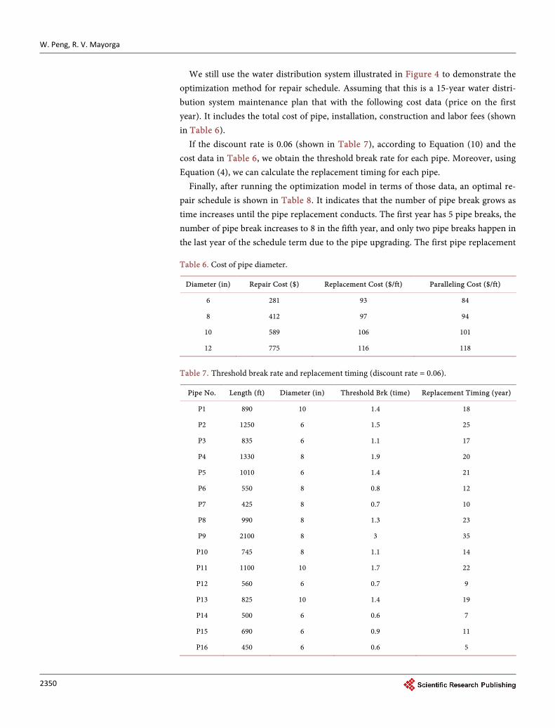
We still use the water distribution system illustrated in Figure 4 to demonstrate the optimization method for repair schedule. Assuming that this is a 15-year water distri-bution system maintenance plan that with the following cost data (price on the first year). It includes the total cost of pipe, installation, construction and labor fees (shown in Table 6).

If the discount rate is 0.06 (shown in Table 7), according to Equation (10) and the cost data in Table 6, we obtain the threshold break rate for each pipe. Moreover, using Equation (4), we can calculate the replacement timing for each pipe.

Finally, after running the optimization model in terms of those data, an optimal re-pair schedule is shown in Table 8. It indicates that the number of pipe break grows as time increases until the pipe replacement conducts. The first year has 5 pipe breaks, the number of pipe break increases to 8 in the fifth year, and only two pipe breaks happen in the last year of the schedule term due to the pipe upgrading. The first pipe replacement

Table 6. Cost of pipe diameter.

Diameter (in) Repair Cost ($) Replacement Cost ($/ft) Paralleling Cost ($/ft)

6 281 93 84

8 412 97 94

10 589 106 101

12 775 116 118

Table 7. Threshold break rate and replacement timing (discount rate = 0.06).

Pipe No. Length (ft) Diameter (in) Threshold Brk (time) Replacement Timing (year)

P1 890 10 1.4 18

P2 1250 6 1.5 25

P3 835 6 1.1 17

P4 1330 8 1.9 20

P5 1010 6 1.4 21

P6 550 8 0.8 12

P7 425 8 0.7 10

P8 990 8 1.3 23

P9 2100 8 3 35

P10 745 8 1.1 14

P11 1100 10 1.7 22

P12 560 6 0.7 9

P13 825 10 1.4 19

P14 500 6 0.6 7

P15 690 6 0.9 11

P16 450 6 0.6 5

W. Peng, R. V. Mayorga

2351

Table 8. The optimal repair schedule.

Year Repair Replace Paralleling

1 P1; P9; P10; P11; P13

2 P1; P9; P10; P11; P13; P2

3 P1; P9; P10; P11; P13; P2

4 P1; P9; P10; P11; P13; P2; P4

5 P1; P9; P10; P11; P13; P2; P4; P9

6 P1; P9; P10; P11; P13; P2; P4; P9

7 P1; P9; P10; P11; P13; P2; P4; P9

8 P1; P9; P10; P11; P13; P2; P4; P9

9 P1; P2; P4; P10; P11; P13 P9(8")

10 P1; P2; P4; P10; P11; P13

11 P1; P2; P4; P10; P11; P13

12 P1; P2; P4; P10; P11 P13(8")

13 P1; P2; P4; P10; P11

14 P1; P2; P3; P4; P11 P10(10")

15 P3; P11 P2(6") P4(8")

P1(6")

Total Cost $(Price on the first year) 471,933

occurs in the ninth year that pipe P9 is replaced by an 8-inch diameter pipe. Only one paralleling pipe is built in the fifteenth year of the schedule term. The total cost of this schedule is $471,933.

4. Conclusion

The paper successfully developed an innovative approach to optimize the rehabilitation & upgrading schedule for water distribution systems based on the stochastic hydraulic reliability assessment. The approach considered the uncertainty of hydraulic parame-ters and treated them as random numbers following the normal distribution. The hy-draulic probability was computed by using the Monte Carlo simulation technique and incorporated EPANET simulation software in MATLAB. This approach subdivided the high complexity WDS optimization problem into two stages—one stage for hydraulic performance optimization and another for mechanical performance optimization. The optimizations of two stages were performed separately but exchanged information with each other. Simultaneously, the threshold break rate model and the genetic algorithm participated in this optimization process. Two practical codes, the hydraulic probability assessment and the RUS schedule, were developed based on this approach and applied for a benchmark water distribution system. The results demonstrated the applicability of this approach.

References [1] Prasad, T.D. and Park, N.-S. (2004) Multi-Objective Genetic Algorithms for Design of Wa-

W. Peng, R. V. Mayorga

2352

ter Distribution Networks. Journal of Water Resources Planning and Management (ASCE), 130, 73-82. https://doi.org/10.1061/(ASCE)0733-9496(2004)130:1(73)

[2] Mays, L.W. (1996) Review of Reliability Analysis of Water Distribution Systems. Stochastic Hydraulics ’96, Balkema, Rotterdam, 53-62.

[3] Goulter, I. (1995) Analytical and Simulation Models for Reliability Analysis in Water Dis-tribution Systems. In: Cabrera, E. and Vela, A., Eds., Improving Efficiency and Reliability in Water Distribution Systems, Kluwer Academic Publishers, Dordrecht, 235-266. https://doi.org/10.1007/978-94-017-1841-7_10

[4] Cullinan, M.J. (1989) Methodologies for the Evaluation of Water Distribution System Re-liability/Availability. Thesis Presented to the Department of Civil Engineering, University of Texas, Austin.

[5] Peng, W. and Mayorga, R.V. (2008) Assessing Traffic Noise Impact Based on Probabilistic and Fuzzy Approaches under Uncertainty. Stochastic Environmental Research and Risk Assessment, 22, 541-550. https://doi.org/10.1007/s00477-007-0173-7

[6] Bao, Y. and Mays, L.M. (1990) Model for Water Distribution System Reliability. Journal of Hydraulic Engineering, 116, 1119-1137. https://doi.org/10.1061/(ASCE)0733-9429(1990)116:9(1119)

[7] Madsen, H.O., Krenk, S. and Lind, N.C. (1986) Methods of Structural Safety. Prentice-Hall, Englewood Cliffs.

[8] Xu, C. and Goulter, I.C. (1998) Probabilistic Model for Water Distribution Reliability. Journal of Water Resources Planning and Management, 124, 218-228. https://doi.org/10.1061/(ASCE)0733-9496(1998)124:4(218)

[9] EPANET (2008) Hydraulic Simulation Software. https://www.epa.gov/water-research/epanet

[10] Quiondry, Q.E., Liebman, J.C. and Brill, E.D. (1981) Optimization of Looped Water Dis-tribution Systems. Journal of Environmental Engineering Division, 107, 665-679.

[11] Lansey, K.E., Duan, N. and Mays, L.W. (1989) Water Distribution System Design under Uncertainties. Journal of Water Resources Planning and Management (ASCE), 115, 630- 644. https://doi.org/10.1061/(ASCE)0733-9496(1989)115:5(630)

[12] Tolson, B.A., Maier, H.R., Simpson, A.R. and Lence, B.J. (2004) Genetic Algorithms for Re-liability-Based Optimization of Water Distribution Systems. Journal of Water Resources Planning and Management (ASCE), 130, 63-72. https://doi.org/10.1061/(ASCE)0733-9496(2004)130:1(63)

[13] Prasad, T.D. and Park, N.S. (2004) Multi-Objective Genetic Algorithms for Design of Water Distribution Networks. Journal of Water Resources Planning and Management (ASCE), 130, 73-82. https://doi.org/10.1061/(ASCE)0733-9496(2004)130:1(73)

[14] Peng, W., Mayorga, R.V. and Imran, S. (2012) A Rapid Fuzzy Optimization Approach to Source Water Blending Problems in Water Distribution Systems. Urban Water Journal, 9, 177-187. https://doi.org/10.1080/1573062X.2011.652133

[15] Peng, W., Mayorga, R.V. and Imran, S. (2012) A Robust Optimization Approach for Real- Time Multiple Source Water Blending Problem. Journal of Water Supply: Research and Technology, 61, 111-122. https://doi.org/10.2166/aqua.2012.037

[16] Savic, D.A. and Walters, G.A. (1997) Genetic Algorithms for Least-Cost Design of Water Distribution Systems. Journal of Water Resources Planning and Management (ASCE), 123, 67-77. https://doi.org/10.1061/(ASCE)0733-9496(1997)123:2(67)

[17] Shamir, U. and Howard, C.D.D. (1979) An Analytic Approach to Scheduling Pipe Re-placement. Journal-American Water Works Association, 71, 248-258.

W. Peng, R. V. Mayorga

2353

[18] Deb, A.K., Hasit, Y., Grablutz, F. and Herz, R. (1988) Quantifying Future Rehabilitation and Replacement Needs of Water Mains. American Water Works Association Research Foundation, Denver.

[19] Ascher, H. and Feingold, H. (1984) Repairable Systems Reliability. Marcel Dekker, NY.

[20] Alperovits, E. and Shamir, U. (1977) Design of Optimal Water Distribution Systems. Water Resources Research, 13, 885-900. https://doi.org/10.1029/WR013i006p00885

[21] Sharp, W.W. and Walski, T.M. (1988) Predicting Internal Roughness in Water Mains. Journal of American Water Works Association, 80, 34-40.

[22] Dandy, G.C., Mcbean, E.A. and Hutchinson, B.G. (1985) Pricing and Expansion of a Water Supply System. Journal of Water Resources Planning and Management, 111, 24-41. https://doi.org/10.1061/(ASCE)0733-9496(1985)111:1(24)

[23] Goldberg, D. (1989) Genetic Algorithms in Search, Optimization, and Machine Learning, Addison-Wesley, New York.

[24] Al-Zahrani, M. and Syed, J.L. (2004) Hydraulic Reliability Analysis of Water Distribution System. Journal of the Institution of Engineers, 1, 76-92.

[25] Yannopoulos, S. and Spiliotis, M. (2013) Water Distribution System Reliability Based on Minimum Cut-Set Approach and the Hydraulic Availability. Water Resources Manage-ment, 27, 1821-1830. https://doi.org/10.1007/s11269-012-0163-5

[26] Jung, D. and Lansey, K. (2014) Water Distribution System Burst Detection Using a Nonli-near Kalman Filter. Journal of Water Resources Planning and Management, 141, 04014070. https://doi.org/10.1061/(ASCE)WR.1943-5452.0000464

Submit or recommend next manuscript to SCIRP and we will provide best service for you:

Accepting pre-submission inquiries through Email, Facebook, LinkedIn, Twitter, etc. A wide selection of journals (inclusive of 9 subjects, more than 200 journals) Providing 24-hour high-quality service User-friendly online submission system Fair and swift peer-review system Efficient typesetting and proofreading procedure Display of the result of downloads and visits, as well as the number of cited articles Maximum dissemination of your research work

Submit your manuscript at: http://papersubmission.scirp.org/ Or contact am@scirp.org