hydraulic balancing and comparison …tesi.cab.unipd.it/48161/1/tesi_bonvicini.pdfuniversity of...
TRANSCRIPT

UNIVERSITY OF PADUA FACULTY OF ENGINEERING
MASTER'S DEGREE IN ENERGETIC ENGINEERING
HYDRAULIC BALANCING AND COMPARISON BETWEEN FAN COIL AND UNDERFLOOR HEATING SYSTEMS
Supervisor: Prof. Michele De Carli Author: Daniele Bonvicini
Co-Supervisor: Dr. Hàmori Sandor Mat. 1058665
A.Y. 2014/2015


2


4
Table of Contents
1. SUMMARY .......................................................................................................................................................... 10
2. INTRODUCTION ABOUT FLUID MECHANICS ....................................................................................................... 10
2.1. Newtonian and Non-Newtonian Fluids .............................................................................................................. 10
2.2. Main properties of fluids .................................................................................................................................... 12
2.2.1. Density ................................................................................................................................................................ 12
2.2.2. Specific weight .................................................................................................................................................... 12
2.2.3. Specific gravity .................................................................................................................................................... 13
2.2.4. Vapor pressure ................................................................................................................................................... 13
2.3. Fluid’s Flows........................................................................................................................................................ 13
2.4. The Bernoulli Equation ....................................................................................................................................... 15
2.5. Fluid’s Losses ...................................................................................................................................................... 17
2.5.1. Major Losses ....................................................................................................................................................... 18
2.5.2. Minor Losses ....................................................................................................................................................... 19
3. VALVES ................................................................................................................................................................ 25
3.1. Valve’s characteristic .......................................................................................................................................... 26
3.1.1. The globe valve ................................................................................................................................................... 28
3.1.2. The equal percentage valve ................................................................................................................................ 29
3.2. Flow coefficient .................................................................................................................................................. 33
3.3. Authority of a valve ............................................................................................................................................ 33
4. PUMPS ................................................................................................................................................................ 37
4.1. Pump curve ......................................................................................................................................................... 37
4.1.1. Efficiency curve ................................................................................................................................................... 40
4.1.2. Net Positive Suction Head (NPSH) ...................................................................................................................... 41
4.2. Cavitation ............................................................................................................................................................ 42
4.3. Pumps in systems ............................................................................................................................................... 42
4.3.1. Pumps arranged in series or in parallel .............................................................................................................. 44
4.3.2. Resistance connected in series or parallel .......................................................................................................... 44
4.3.3. Open and closed systems ................................................................................................................................... 45
4.4. Regulation of pumps ........................................................................................................................................... 47
4.4.1. Throttle regulation.............................................................................................................................................. 47
4.4.2. Regulation with bypass valve ............................................................................................................................. 48
4.4.3. Regulation by speed variation ............................................................................................................................ 49
5. HYDRAULIC BALANCING ..................................................................................................................................... 50
5.1. Fundamental concepts underlying balancing ..................................................................................................... 50
5.1.1. The effect of flow rate on heat output ............................................................................................................... 50
5.1.2. Each crossover affects other crossovers............................................................................................................. 53

5.1.3. Direct vs reverse return piping ........................................................................................................................... 53
5.2. Types of balancing devices ................................................................................................................................. 55
5.2.1. Balancing valves .................................................................................................................................................. 55
5.2.1.1. Dynamic balancing valves: autoflow ........................................................................................................... 56
5.2.1.2. Static balancing valve .................................................................................................................................. 57
5.2.1.3. Differential pressure control valves ............................................................................................................ 59
5.2.2. Hydraulic separator ............................................................................................................................................ 60
6. PRACTICAL EXAMPLE OF HYDRAULIC BALANCING ............................................................................................. 64
6.1. The system .......................................................................................................................................................... 64
6.2. Balancing the system .......................................................................................................................................... 64
6.3. The unbalanced system ...................................................................................................................................... 70
7. UNDERFLOOR HEATING SYSTEM ........................................................................................................................ 74
7.1. Design the underfloor heating system ............................................................................................................... 74
8. COMPARISON BETWEEN FAN COIL SYSTEM AND UNDERFLOOR HEATING SYSTEM .......................................... 78
9. CONCLUSION ...................................................................................................................................................... 79
Bibliography ...................................................................................................................................................................... 80
List of Pictures
Figure 1 Fluid between two plates with a force F applied on the top plate ..................................................................... 10
Figure 2 Shearing stress versus rate of shearing strain for non-newtonian fluid ............................................................. 12
Figure 3 Velocity trend for an ideal fluid flowing in a pipe ............................................................................................... 13
Figure 4 Velocity trend for a real fluid flowing in a pipe................................................................................................... 14
Figure 5 Representation of the reynolds dye experiment ................................................................................................ 14
Figure 6 Turbulent, transient and laminar flow in a pipe ................................................................................................. 15
Figure 7 EL and HGL in a pipe ........................................................................................................................................... 17
Figure 8 Use of the HGL to define the pressure in the pipe ............................................................................................. 17
Figure 9 Moody’s chart ..................................................................................................................................................... 19
Figure 10 Sudden enlargement in a pipe .......................................................................................................................... 20
Figure 11 Sudden constriction in a pipe ........................................................................................................................... 20
Figure 12 Different types of valves: a) plug and seat three-port mixing valve, ................................................................ 25
Figure 13 diverting and mixing valves............................................................................................................................... 26
Figure 14 Three-port terminology, showing the name of the ports ................................................................................. 26
Figure 15 Radiator heat output as function of flow rate, with temperature as parameter ............................................. 27
Figure 16 Representation of valve’s characteristics ......................................................................................................... 27
Figure 17 the shape of the plug determines the valve characteristic............................................................................... 28

6
Figure 18 schematic representation of a globe valve ....................................................................................................... 28
Figure 19 quick opening characteristic ............................................................................................................................. 29
Figure 20 Theoretical (dotted line) and pratcical (solid line) ............................................................................................ 30
Figure 21 equal percentage characteristic ....................................................................................................................... 31
Figure 22 heat output vs stem position relationship with an equal percentage valve..................................................... 31
Figure 23 two different ways to obtain an equal percentage characteristic .................................................................... 32
Figure 24 sequence of stem lift in equal percentage valves ............................................................................................. 32
Figure 25 pressure drop-flow diagram with kv as parameter ........................................................................................... 33
Figure 26 flow through a control valve as function of spindle lift, showing the effect of valve authority ....................... 34
Figure 27 valve authority diagrams showing three-port valves and pressure drop in the circuit .................................... 34
Figure 28 A three-port valve with balancing valve in the bypass leg ............................................................................... 35
Figure 29 curves for symmetrical three-port valve selected for linear power output ..................................................... 35
Figure 30 curves for asymmetrical three-port valve selected for linear power output ................................................... 36
Figure 31 schematic representation of a centrifugal pump ............................................................................................. 37
Figure 32 Schematic view of the fluid path inside a centrifugal pump ............................................................................. 37
Figure 33 velocity diagram at the inlet and exit of a centrifugal pump ............................................................................ 38
Figure 34 head-flowrate curve for a centrifugal pump showing the effects of losses ..................................................... 39
Figure 35 characteristic curve for different rotating velocities (n1>n2>n3) ..................................................................... 40
Figure 36 typical performance characteristic for a centrifugal pump .............................................................................. 41
Figure 37 diagram showing NPSHR, efficiency, power and head curve of a pump ........................................................... 42
Figure 38 typical flow system ........................................................................................................................................... 43
Figure 39 pump and system curves used to obtain the operating point for the system .................................................. 43
Figure 40 parallel-connected pumps ................................................................................................................................ 44
Figure 41 series-connected pumps ................................................................................................................................... 44
Figure 42 resistances connected in series ........................................................................................................................ 45
Figure 43 resistences connected in parallel ...................................................................................................................... 45
Figure 44 system curve for a closed system ..................................................................................................................... 46
Figure 45 open system with positive geodetic lift ............................................................................................................ 46
Figure 46 open system with negative geodetic lift ........................................................................................................... 47
Figure 47 Pump regulation by throttle configuration ....................................................................................................... 48
Figure 48 power saving with throttle regulation .............................................................................................................. 48
Figure 49 pump regulation by bypass valve ..................................................................................................................... 48
Figure 50 the bypass valve does not provide a power saving .......................................................................................... 49
Figure 51 variable speed regulation ................................................................................................................................. 49
Figure 52 a typical system with a heat source, some crossovers and heating loads ........................................................ 51
Figure 53 effect of the flowrate on the heat output of a heat emitter ............................................................................ 52

Figure 54 heat output vs flowrate through a heat emitter .............................................................................................. 52
Figure 55 Desirable systems should have differential pressure control ........................................................................... 53
Figure 56 Undesirable systems do not have differential pressure control ....................................................................... 53
Figure 57 Direct return system ......................................................................................................................................... 54
Figure 58 Direct return system with balancing valves ...................................................................................................... 54
Figure 59 Reverse return system ...................................................................................................................................... 54
Figure 60 Reverse return piping for multiple panel radiators .......................................................................................... 55
Figure 61 autoflow balancing valve .................................................................................................................................. 56
Figure 62 mode of operation of an autoflow ................................................................................................................... 57
Figure 63 mode of operation of a manual balancing valve .............................................................................................. 58
Figure 64 working principle of a flowmeter valve: setting the reference flowrate, let the spring lift to its maximum
value and finally adjust the spring position the desired position ..................................................................................... 59
Figure 65 Working principle of a Dpcv .............................................................................................................................. 60
Figure 66 differential pressure control valve .................................................................................................................... 60
Figure 67 system with a boiler and three circulating pumps ............................................................................................ 61
Figure 68 system with hydraulic separator....................................................................................................................... 62
Figure 69 three possible working conditions of a hydraulic separator............................................................................. 62
Figure 70 model of the shopping center with his own heating system ............................................................................ 64
Figure 71 technical diagram of pressure drop-flow rate .................................................................................................. 65
Figure 72 Flow rate modification ...................................................................................................................................... 72
Figure 73Heat output modification .................................................................................................................................. 73
Figure 74 pressure loss in PEX tube .................................................................................................................................. 75
Figure 75Manifold pressure drops.................................................................................................................................... 76
Figure 76 sketch of the underfloor heating circuit piping system .................................................................................... 77
Figure 77 manifold total pressure drops .......................................................................................................................... 77
List of tables
Table 1 Some typical value of minor losses ...................................................................................................................... 20
Table 2 Minor losses for different type of valves ............................................................................................................. 21
Table 3 minor losses coefficients for pipe components ................................................................................................... 22
Table 4 minor losses coefficients for pipe fittings ............................................................................................................ 23
Table 5 minor losses calculation ....................................................................................................................................... 24
Table 6 flow rate calculation............................................................................................................................................. 65
Table 7 Major losses calculation, linear major pressure drop .......................................................................................... 66
Table 8 Major losses calculation, actual major pressure drop ......................................................................................... 67
Table 9 Minor losses calculation ....................................................................................................................................... 68
Table 10 Total pressure drops calculation ........................................................................................................................ 69

8
Table 11 pressure drop between emitters and boiler ...................................................................................................... 69
Table 12 balancing valves type and position .................................................................................................................... 70
Table 13 pump characteristics with fan coil system ......................................................................................................... 70
Table 14 results of unbalanced system on the flow rate .................................................................................................. 71
Table 15 results of unbalanced system on return temperature ....................................................................................... 72
Table 16 Underfloor heating system specific power ........................................................................................................ 74
Table 17 supply and return temperature calculation ....................................................................................................... 74
Table 18manifold pressure drop calculation .................................................................................................................... 76
Table 19 Pump characteristics with underfloor heating system ...................................................................................... 77
Table 20 load factor and working hours ........................................................................................................................... 78
Table 21 pumps electrical absorption .............................................................................................................................. 78

10
1. SUMMARY
The first goal of this thesis it to analyze the benefits obtained through a correct hydraulic balancing of a hydraulic
heating system, and the problems caused by an incorrect balancing. This goal has been chosen because even today a
large number of heating systems are installed and are operating without a correct balancing, especially in residential
plants, therefore causing discomfort to the users.
The second part of the thesis is focused on the comparison between a fan coil heating system and an underfloor
heating system. To do so have been taking into account parameters like the load factor and the electrical absorption
of the pump used to circulate the heating fluid in the two systems.
Despite being a very simple procedure to pull off, the results show that the effects of an incorrect hydraulic balancing,
like the modification in flow rate through the emitters and their heat output, highly affect the quality of the internal
air and the health of the heating system.
2. INTRODUCTION ABOUT FLUID MECHANICS
Fluid mechanics is that discipline that is concerned with the behavior of fluids (gases and liquids) at rest or in
movement. It covers a vast array of phenomena that occur in nature, in biology and also in engineering processes.
Fluids are widely used in all engineering fields: we can get energy from them, we can use them to transport energy
from one place to another one and also we can use them to warm and cool down buildings.
Therefore it’s extremely important to study the features and the behavior of the fluids, how they flow in a pipe, how
they can transport energy e how they loss energy to the environment. Almost every engineering plant in the world use
a fluid, thus we must know how to use them properly.
2.1. Newtonian and Non-Newtonian Fluids All fluids can be divided in two main categories: Newtonian and non-Newtonian fluids. The difference between these
two typologies of fluids stands on the behavior of their viscosity.
As we know the viscosity of a fluid is a parameter which evaluates a fluid’s resistance to flow or, in other words, it is a
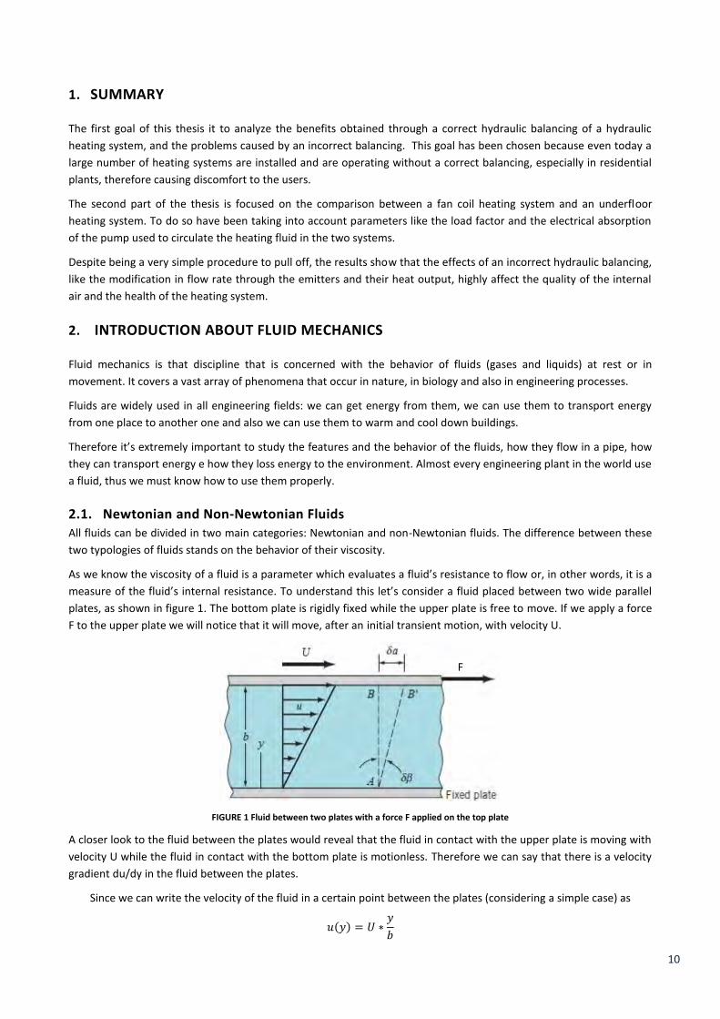
measure of the fluid’s internal resistance. To understand this let’s consider a fluid placed between two wide parallel
plates, as shown in figure 1. The bottom plate is rigidly fixed while the upper plate is free to move. If we apply a force
F to the upper plate we will notice that it will move, after an initial transient motion, with velocity U.
FIGURE 1 Fluid between two plates with a force F applied on the top plate
A closer look to the fluid between the plates would reveal that the fluid in contact with the upper plate is moving with
velocity U while the fluid in contact with the bottom plate is motionless. Therefore we can say that there is a velocity
gradient du/dy in the fluid between the plates.
Since we can write the velocity of the fluid in a certain point between the plates (considering a simple case) as
𝑢(𝑦) = 𝑈 ∗𝑦
𝑏
F

we would fine that the gradient is a constant
𝑑𝑢
𝑑𝑦=
𝑈
𝑏
In a small time increment dt, an imaginary vertical line AB in the fluid would rotate through an angle d so that:
tan d ≈ d =𝑑𝑎
𝑏
and since
𝑑𝑎 = 𝑈 ∗ 𝑑𝑡
it comes that
d =𝑈 ∗ 𝑑𝑡
𝑏
As we can see we can’t relate d only with U (and so F) because it’s a function of time too. Thus it’s reasonable to
consider not the shearing strain, but the rate of shearing strain (or rate of angular deformation)
�̇� = lim𝑑𝑡→0
d
𝑑𝑡
which can be written as
�̇� =𝑈
𝑏=
𝑑𝑢
𝑑𝑦
Experimental analysis proved that the rate of shearing stray is increased in direct proportion with the shearing stress τ
as
τ ∝ �̇�
or
τ ∝ 𝑑𝑢
𝑑𝑦
For common fluids such as water, oil and air this relation can be written as
τ = μ 𝑑𝑢
𝑑𝑦
where the constant of proportionally is called absolute (or dynamic) viscosity. Fluids with a constant viscosity are
called Newtonian fluids while fluids for which the shearing stress is not linearly related to the rate of shearing strain
are called non-Newtonian fluids. A representation of both types of fluid is shown in figure 2.

12
FIGURE 2 Shearing stress versus rate of shearing strain for non-newtonian fluid
In other words we can say that, in order to have U constant, for the second law of dynamics there must be a force F’
between the fluid and the upper plate, that is
�̅� = −𝐹′̅
or, using scalar values
𝐹 = 𝐹′
Now, being A the surface of the moving plate, it can be experimentally proved that
𝐹 = 𝐹′ ∝𝑢𝐴
𝑏
The constant of proportionality is the dynamic viscosity of the fluid, so
𝐹 = 𝐹′ = μ 𝑢𝐴
𝑏
Using the International System (SI) the dynamic viscosity’s unit of measure is Kg/m*s but it can be used also the Poise
(1 P = 10-1
Kg/ms)
In this thesis, since the Newtonian fluids are easier to discuss and more common than the non-Newtonian, we will
refer only to them.
2.2. Main properties of fluids Apart from dynamic viscosity there are other properties of the fluids that are important to discuss about.
2.2.1. Density The density of a fluid is defined as his mass per unit volume and its unit of measure is then Kg/m
3
=𝑚
𝑉
The value of density can vary between different types of fluids. For liquids its value varies very little
with temperature and pressure variations while for gases it’s the opposite.
The specific volume is the volume per unit mass and is therefore the reciprocal of the density
𝑣 =1
2.2.2. Specific weight The specific weight of a fluid is defined as its weight per unit volume, so it can be written as

𝛾 =𝑚𝑔
𝑣= 𝑔
and its unit of measure is N/m3. As density is used to characterize the mass of a system, the specific
weight is used to characterize the weight of the system.
2.2.3. Specific gravity The specific gravity of a fluid is defined as the ratio of the density of the fluid and the density of the
water at a fixed temperature (usually 4°C, so the density will be 1000 Kg/m3)
𝑆𝐺 =
𝐻2𝑂,4°𝐶
2.2.4. Vapor pressure The vapor pressure of a fluid is defined as the equilibrium pressure of a gas above its liquid (or solid). When in
a container with fluid inside and a vacuum space above it the number of molecules evaporating is equal to
the number entering the fluid the vapor is said to be saturated and the pressure exerts on the liquid surface is
the vapor pressure.
Since the vapor pressure depends on the molecular activity, the vapor pressure of a specific fluid depends on
temperature.
2.3. Fluid’s Flows It is possible, and useful, to categorize the type of flow that a fluid can have. If we look, for example, to a flowing river
we will notice that the flow of the liquid is very complex to describe since the velocity varies from one point to
another.
Under some circumstances the flow will not be as variable as this; in effect we can describe the flow of a liquid using
these four categories:
- Uniform flow: if the velocity has the same magnitude and direction in every point in the fluid.
- Non uniform flow: if at a given instant the velocity is not the same in every point in the fluid.
- Steady: the steady flow is one in which the conditions (as velocity, pressure etc.) may change between
two points but do not change in time.
- Non steady: if at any point in the fluid the conditions change in time the flow is called non-steady.
Speaking about real fluids we have to consider the viscosity’s effects. In an ideal flow, as illustrated in figure 3, the
velocity in a cross section of the pipe remain constant because there is no friction between the fluid and the wall of
the pipe and between the particles of the fluid.
FIGURE 3 Velocity trend for an ideal fluid flowing in a pipe
The pressure before the considered cross section will be equal to the one after the same section, thus we can say that
in an ideal case there is no need for a pressure difference to have flow.
u

14
On the other hand, in a real flow we know that the velocity of the fluid in proximity to the wall must be zero. Then we
will have a non- linear velocity in the cross section, as we can see in figure 4.
FIGURE 4 Velocity trend for a real fluid flowing in a pipe
In this case we have a difference of pressure between the liquid before and after the cross section, and we need this
difference to have the flow. Due to the friction losses we will have that:
𝑝𝑎 > 𝑝𝑏
In a real situation we can distinguish three different kind of flow: turbulent, laminar and transitional.
To study these flows we can refer to the Reynolds’ dye experiment, depicted in figure 5. Osborne Reynolds (1842-
1912), a British scientist and mathematician, was the first to distinguish the differences between these flows injecting
dye into a pipe in which water flowed due to gravity.
FIGURE 5 Representation of the reynolds dye experiment
Reynolds observed that:
- For “small enough flow rates” the dye streak remained as well-defined as it flowed along.
- For “intermediate flow rates” the dye streak fluctuated in both time and space, and irregular burst of
intermittent behavior appeared along the streak.
- For “large enough flow rates” the dye streak most immediately became blurred and spread across the
whole pipe.
After many experiments Reynolds found that we can somehow predict the flow of a fluid using a dimensionless ratio,
known as Reynolds number:
𝑅𝑒 =𝑈𝐷
𝜇
where U is the average velocity in the pipe, and D is the diameter of the pipe. We can instantly notice that not only
the velocity of the fluid influences the flow type, but also the shape of the pipe and the fluid’s properties.
The distinction between the three different flows can be based on the value of the Reynolds number but we have to
remember that the ranges for which laminar, turbulent and transient flow are obtained cannot be precisely given. For
general engineering purpose we can assume that:
Q=UA
u

Turbulent flow: Re>4000
Transient flow: 2100<Re<4000
Laminar flow: Re<2100
FIGURE 6 Turbulent, transient and laminar flow in a pipe
2.4. The Bernoulli Equation One of the most important tools in fluid mechanics is definitely the Bernoulli equation.
Thanks to the energy conservation, when friction is negligible, we can affirm that the sum of kinetic and potential
energy is constant.
Kinetic energy: 1
2𝑚𝑢2
Potential energy: 𝑚𝑔𝑦
Under some restrictions, such as:
- Flow is steady
- Density is constant (fluid is incompressible)
- Friction losses are negligible
- We refer to states at two points in the same streamline
we can write the Bernoulli equation, that is
𝑝1 +1
2𝑢1
2 + 𝑔𝑦1 = 𝑝2 +1
2𝑢2
2 + 𝑔𝑦2
It’s important to know that all the restrictions are impossible to satisfy at any instant in time but fortunately for many
real situations where the conditions are approximately satisfied, the equation gives good results.
To explain this equation in a simple way we can imagine a pipe (which have different width and elevation between its
beginning and its end) with a fluid inside which is flowing from a starting position to a final one. For the
incompressibility of the fluid the volume of the entering fluid must be equal to the one of the outgoing fluid:
𝑉 = 𝐴1𝑥1 = 𝐴2𝑥2
Where A is the area of the entrance (and exit) of the pipe and x is the length cover by the fluid. The fluid mass is
𝑚 = 𝑉
Due to the movement of the fluid the mass 𝑚 of it in the period t has moved from the initial height y1 to y2 and its
velocity has changed from u1 to u2.
From point 1 to point 2 we have therefore a variation in kinetic and potential energy:

16
𝐸𝑘 =1
2(𝑚)𝑢2
2 −1
2(𝑚)𝑢1
2 =1
2𝑉(𝑢2
2 − 𝑢12)
𝐸𝑝 = 𝑚𝑔𝑦2 − 𝑚𝑔𝑦1 = 𝑉𝑔(𝑦2 − 𝑦1)
The fluid before the section A1 executes a force F1=p1A1 (where p1 is the pressure on section A1) on the entering mass
𝑚. The result of this force is a work:
𝐿1 = 𝐹1𝑥1 = 𝑝1𝐴1𝑥1 = 𝑝1𝑉
Similarly, at the end of the pipe, there is a force F2 which produces a work as:
𝐿2 = −𝐹2𝑥2 = −𝑝2𝐴2𝑥2 = −𝑝2𝑉
The total work produced by the two forces is then:
𝐿𝑡𝑜𝑡 = 𝐿1 + 𝐿2 = 𝑝1𝑉 − 𝑝2𝑉 = (𝑝1 − 𝑝2)𝑉
From the kinetic energy theorem we can also say that:
𝐿𝑡𝑜𝑡 = 𝐸𝑘 + 𝐸𝑝
Merging the two expressions for Ltot the result we get is:
(𝑝1 − 𝑝2)𝑉 =1
2𝑉(𝑢2
2 − 𝑢12) + 𝑉𝑔(𝑦2 − 𝑦1)
Dividing all the terms per V and explicating all the terms with the subscript 1 we finally get the well-known
expression of the Bernoulli equation:
𝑝1 +1
2𝑢1
2 + 𝑔𝑦1 = 𝑝2 +1
2𝑢2
2 + 𝑔𝑦2
Or, in other words:
𝑝 +1
2𝑢2 + 𝑔𝑦 = 𝑐𝑜𝑠𝑡𝑎𝑛𝑡
The terms 𝑝 + 𝑔𝑦, since they’re present even without flow, are called static pressure while the term 1
2𝑢2 is called
dynamic pressure.
A useful interpretation of the Bernoulli equation can be obtained through the use of the concepts of the hydraulic
grade line (HGL) and the energy line (EL). Dividing all terms of the Bernoulli equation by the specific weight allows us
to write the equation in a “height form”:
𝑝
𝛾+
𝑢2
2𝑔+ 𝑦 = 𝑐𝑜𝑠𝑡𝑎𝑛𝑡 = 𝐻
In this expression all the terms have the unit of a length and represent a certain head: 𝑝
𝛾 is the pressure head,
𝑢2
2𝑔 is the
velocity head and y is the elevation head. The sum of these three terms is called total head H.
The energy line (EL) is a line that represents the total energy available to the fluid, which means that it’s a geometrical
representation of H.
The sum of the elevation and pressure head is often termed piezometric head. It allows us calculating the hydraulic
grade line HGL as the difference between the energy line and the piezometric line.
Summarizing we have:
𝐸𝐿 ≡𝑝
𝛾+
𝑢2
2𝑔+ 𝑦 = 𝐻
𝑃𝑖𝑒𝑧𝑜𝑚𝑒𝑡𝑟𝑖𝑐 ℎ𝑒𝑎𝑑 ≡𝑢2
2𝑔+ 𝑦
𝐻𝐺𝐿 ≡ 𝐸𝐿 − 𝑃𝑖𝑒𝑧𝑜𝑚𝑒𝑡𝑟𝑖𝑐 ℎ𝑒𝑎𝑑

An illustration of these heads is shown in figure 7.
FIGURE 7 EL and HGL in a pipe
Using these heads is particularly useful when we have to analyze a pipe connected to a tank as the distance between
the HGL and the pipe indicates the pressure inside the pipe. As we can see in figure 8 if the HGL is above the pipe the
pressure inside the pipe will be positive (above atmospheric). If the HGL is under the pipe the pressure inside the pipe
will be negative (under atmospheric).
FIGURE 8 Use of the HGL to define the pressure in the pipe
2.5. Fluid’s Losses For an ideal fluid flowing in a pipe the energy line maintains constant through the pipe, but when we consider a real
fluid this is not true due to the losses caused by the viscosity. This means that we have to calculate the so called head
losses, hL.
A typical pipe system usually consists in various lengths of straight pipes connected with other elements as valves and
elbows. The overall head loss is the combination of the losses that occur in the straight pipes, the major losses hL,major,
and the head loss in the various elements, the minor losses hL,minor:
ℎ𝐿 = ℎ𝐿,𝑚𝑎𝑗𝑜𝑟 + ℎ𝐿,𝑚𝑖𝑛𝑜𝑟
These losses have to be considered in the energy equation, which can be written as:
𝑝1
𝛾+
𝑢12
2𝑔+ 𝑦1 =
𝑝2
𝛾+
𝑢22
2𝑔+ 𝑦2 + ∑ ℎ𝑆 + ∑ ℎ𝐿
where hS consist of all the addiction and removal heads due to machines placed between section 1 and 2.

18
If the energy equation has to be written in terms of pressure, it will become:
𝑝1 + 𝑢1
2
2+ 𝛾𝑦1 = 𝑝2 +
𝑢22
2+ 𝛾𝑦2 + ∑ ℎ𝑆 + ∑ ℎ𝐿
Obviously the losses must now be written in terms of pressure, not in terms of high.
2.5.1. Major Losses By means of a dimensional analysis
1 is possible to find a semi-empirical way to calculate the pressure drop in a pipe
where a fluid is flowing as long as the flow is turbulent, fully developed and incompressible.
One of the most famous equations in this field is the Darcy-Weisbach, used for smooth pipes:
ℎ𝐿,𝑚𝑎𝑗𝑜𝑟 = 𝑓𝐿
𝐷
𝑢2
2𝑔
where f is the Darcy friction factor and L and D are the length and diameter of the pipe. This loss is written in terms of
height, so it must be used with the properly expression of the energy equation.
In a hydraulic balancing is however more useful to have the losses written in terms of pressure, that is:
ℎ𝐿,𝑚𝑎𝑗𝑜𝑟 = 𝑓𝐿
𝐷
𝑢2
2
The dimensionless coefficient f is the Darcy friction coefficient. It can be proved that it’s a function of the Reynolds
number of the flow and the ratio between the pipe’s diameter and the surface roughness:
𝑓 = 𝐹(𝑅𝑒,𝜀
𝐷)
There are many equations we can use to solve the Darcy friction factor. Two of the most famous are the Colebrook
and the Blasius.
The Colebrook equation is:
1
√𝑓= −2 log(
𝜀 𝐷⁄
3.7+
2.51
𝑅𝑒√𝑓 )
As we can see it’s an implicit equation, thus to solve the friction factor f we will need to do some iterations.
A graphic representation of the Colebrook equation is the so called Moody chart, figure 9:
1 Goodwill I.M., Sleigh P.A., Fluid Flow in Pipes, CIVE2400 Fluid Mechanics, January 2008, pp. 6-12

FIGURE 9 Moody’s chart
The Blasius equation is simpler than the Colebrook’s, since it does not have terms for relative roughness. Nevertheless
this means that this equation can be used only on smooth pipes even if it’s often used in rough pipes because of its
simplicity:
𝑓 =0.316
𝑅𝑒0.25
Under laminar flow it’s been developed another equation to calculate hL,major, called the Hagen-Poiseuille equation:
ℎ𝐿,𝑚𝑎𝑗𝑜𝑟 = 32𝜇𝐿𝑢
𝐷2𝛾
Comparing this equation with the Darcy’s will let us find the equation for the friction factor in laminar flow:
𝑓 =64𝜇
𝑢𝐷=
64
𝑅𝑒
In laminar flow there’s no need for iterations since the friction factor is only a function of the Reynolds number.
2.5.2. Minor Losses In addition to head losses due to friction there are always head losses in pipes due to bends, elbows, valves etc. If for
long pipes their effect can be neglected, for short pipes they have to be taken in account.
A general formula for these kinds of losses is:
ℎ𝐿,𝑚𝑖𝑛𝑜𝑟 = 𝑘𝐿
𝑢2
2𝑔
where kL is a constant which depends on the system’s geometry.
Similarly to the major losses, it’s useful to write the minor losses in terms of pressure:
ℎ𝐿,𝑚𝑖𝑛𝑜𝑟 = 𝑘𝐿𝑢2
2
The value of kL is, most of the time, obtained experimentally:
20
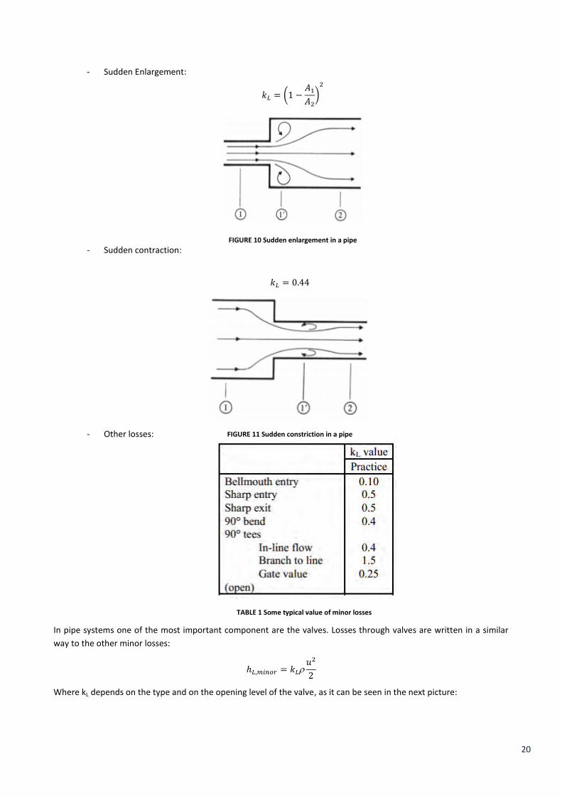
- Sudden Enlargement:
- Sudden contraction:
- Other losses:
TABLE 1 Some typical value of minor losses
In pipe systems one of the most important component are the valves. Losses through valves are written in a similar
way to the other minor losses:
ℎ𝐿,𝑚𝑖𝑛𝑜𝑟 = 𝑘𝐿𝑢2
2
Where kL depends on the type and on the opening level of the valve, as it can be seen in the next picture:
𝑘𝐿 = (1 −𝐴1
𝐴2
)2
FIGURE 10 Sudden enlargement in a pipe
𝑘𝐿 = 0.44
FIGURE 11 Sudden constriction in a pipe

TABLE 2 Minor losses for different type of valves
Minor losses through valves are often given as equivalent length. In this terminology the head losses through a valve is
given as the length of a straight pipe that would produce the same losses as the component, that is (written in terms
of pressure):
ℎ𝐿,𝑚𝑖𝑛𝑜𝑟 = 𝑘𝐿𝑢2
2= 𝑓
𝑙𝑒𝑞
𝐷
𝑢2
2
𝑙𝑒𝑞 =𝑘𝑙
𝑓𝐷
A typical table will however report the value of the ratio leq/D, not the single value of the equivalent length.
This means that, in order to computing the minor losses caused by the presence of a valve in a pipe, the steps to
follow are:
- Find the ratio leq/D for the valve in a table;
- Through the wall roughness and the diameter of the pipe, find the value of the friction factor in the
Moody diagram;
- Compute 𝑘𝑙 = 𝑓(𝑙𝑒𝑞 , 𝐷);
- Compute ℎ𝐿,𝑚𝑖𝑛𝑜𝑟 = 𝑘𝐿𝑢2
2
Another way to evaluate the minor losses in a piping system is the one advised by Caleffi S.p.A.2. They offer two
different tables to refer to (tables 3 and 4). In each table are shown coefficients relating to the flow resistance
introduced by a fitting or particular pipe component basing on the pipe diameter (corners, tees, etc. ).
2 http://www.caleffi.com/italy/it/homepage

22
TABLE 3 Minor losses coefficients for pipe components

TABLE 4 Minor losses coefficients for pipe fittings
With these tables we can calculate the sum of the minor losses coefficients per each section of the piping system,
considering both fittings and pipe components. Once the sum and the fluid velocity in a section are known, by using
another table shown as table 5, it is possible to calculate the total minor pressure drop of that section.

24
TABLE 5 Minor losses calculation

3. VALVES
Valves are one of the most important components in a pipes system. They can be used to control the system pressure,
the amount of flow and even the temperature of the fluid flowing in the system.
Valves may be classified by their function:
- Regulating: a valve which is adjusted during commissioning to provide a fixed resistance in a fluid circuit
to give the design flow rate and ensure the correct balance. The adjustment is normally manual.
- Flow limiting: known as automatic or dynamic balancing valves, they’re utilized to maintain a constant
flow in the circuit regardless the pressure difference across them.
- Differential pressure control: a valve which automatically adjusts to maintain a certain pressure
difference across part of the circuit.
- Modulating: a valve which is adjusted by the control system in order to regulate the hydraulic flow.
- Safety shut-off: a valve which is designed to close under spring pressure in critical condition or out-of-
range process variable.
Modulating valves will be the main subject of this section since they’re the most common type of valves used in
hydraulic circuits.
Several types of valves are used, and the most common are shown figure 12:
FIGURE 12 Different types of valves: a) plug and seat three-port mixing valve, b) rotary shoe valve, c) two part plug and seat valve, d) butterfly valve
Valves are available in two, three or four-port configuration.
Two-port valves are used to throttle fluid in a circuit. Although using a two-ports valve in a complex circuit con lead to
pressure variation and balancing problems throughout the system if the valve is used with variable speed pump and
with proper attention to system design it can assure low first cost and low pumping cost.
Three-port valves have found widespread application especially in HVAC systems, where they’re used with constant
speed pump in order to offer a wide range of well-stablished and trouble-free control system. A three-port valve is
provided with two inlet ports and one outlet port when described as a mixing valve or with one inlet port and two
outlet ports if it’s a diverting valve. An example of mixing and diverting valve is shown in the next figure.

26
FIGURE 13 Diverting and mixing valves
Unfortunately there is not a consistent terminology to describe the ports of a three-port valve. In the next figure the
more common conventions are illustrated.
FIGURE 14 Three-port terminology, showing the name of the ports
3.1. Valve’s characteristic A control valve is one link in a chain of control, running from an error signal which is the input for the controller in
order to change the output of the emitter. Although not necessary, a linear relation between the change in output
from the controller and the output of the emitter are well-recommended in a well-balanced and stable circuit.
However, for most of heat emitters, there is a strongly non-linear relation between the flow rate of the heat fluid and
the heat output of the emitter, with output increasing rapidly from low flow rates and then flattering out for higher
flow rates (i.e. for radiators3) as shown in figure 15.
3 Warburton P., Building Control System, CIBSE Guide, February 2009, p. 3-10

FIGURE 15 Radiator heat output as function of flow rate, with temperature as parameter
A valve which produces a flow rate proportional to spindle lift would therefore result in a non-linear system, operating
in a narrow range of spindle movement with possibly resulting in unstable operations.
For this reason valves are design in order to guarantee that the heat output from the emitter is approximately
proportional to the spindle lift. To do so the plug of the valve is shaped in various way to ensure that the free area (so
the flow rate) is a function of the spindle lift. This defines the characteristic of the valve, and the most common
encountered are:
- Linear: where the orifice area is directly linear with the spindle movement and the flow varies linearly
with the spindle lift.
- Equal percentage: when a percentage variation of valve spindle lift provides an equal percentage change
in orifice area.
- Characterized V-port: characteristic which fall between linear and equal percentage.
- Quick opening: where the flow increase rapidly from zero to a small spindle lift. These valves are used
primarily for on-off service.
All previous characteristics are pictured in figure 16.
FIGURE 16 Representation of valve’s characteristics

28
In order to have those different characteristic curves the plug of the valve must be shaped in different ways, as shown
in picture 17:
FIGURE 17 The shape of the plug determines the valve characteristic
3.1.1. The globe valve A globe valve consists in a body that suddenly changes the direction of flow, as seen in picture 18. Flow enters the
bottom chamber, flows upwards through the gap between the seat and the flat disc and finally exits sideway from the
upper chamber. The gap between the seat and the disc determines the flow resistance created by the valve.
FIGURE 18 Schematic representation of a globe valve
Globe valves should always be installed such that flow enters from the bottom chamber. This allows the disc to close
against the higher pressure chamber. Reverse flow in this type of valve may cause unstable flow regulation, cavitation
and noise.
The movement of the flat disc when the stem is rotated creates the so-called “quick opening” characteristic. This
implies that the flow rate will rapidly increase as the flat disc first lift up from the since, then continues to rise at
progressively slow rates. The characteristic is illustrated in figure 19.

FIGURE 19 Quick opening characteristic
The combination of quick-opening characteristic with the rapid rise in heat transfer rate at low flowrates makes the
overall relationship between heat output and flowrate very non-linear, and hence very difficult to control, especially
at low flowrates.
3.1.2. The equal percentage valve The equal percentage valve has a theoretical characteristic which can be mathematically expressed as an equation
relating the flow with the spindle movement for a constant pressure drop across the valve:
𝑄 = 𝑄0𝑒(𝑆∗𝑛)
where Q is the flow through the valve, Q0 is the theoretical flow through the valve (at S = 0), n is the valve sensitivity
and S is the spindle lift level (1 = fully open, 0 = fully closed).
The sensitivity n is the percentage change in flow through the valve for a 1% change in stem position. The theoretical
flow Q0 is a mathematical convenience and it doesn’t represent the real flow when the valve is closed.
An equal percentage valve is made to follow the theoretical characteristic shown in figure 16 but departs from it at
low flow rates. A practical equal percentage valve has a characteristic curve as shown in figure 20.

30
FIGURE 20 Theoretical (dotted line) and pratcical (solid line)
characteristic curve for an equal percentage valve
Qmin is the minimum flow at which the valve provides reasonable control, under it the flow rate rapidly fall off and
cannot be controlled reliably. For this reason valves are designed to shut off quickly for flows below Qmin. if it’s not
true, the residual flow is called “let-by”.
The ratio of the maximum controllable flow to the maximum flow is called rangeability R. A rangeability of 25 means
that the valve is able to reduce the flow through it down till 4% of its maximum. By this definition it’s obvious how a
good rangeability level is essential when the valve is required to control at low flow rates.
The equal percentage valve has been created to provide a more proportional relationship between heat output and
stem position. Flow through this type of valves increases exponentially with upward movement of the stem. Assuming
that the differential pressure across the valve is held constant, equal increments of stem movement result in an equal
percentage change in current flow through the valve. For example, moving the stem from 40% open to 50% open (a
10% change) will increase the flowrate by 10% from its value at 40% open. This relationship is illustrated in picture 21.

FIGURE 21 Equal percentage characteristic
When a valve with equal percentage characteristic control flow through an heat emitter, the relationship between
heat output from the emitter and stem position becomes nearly linear. As shown in figure 22, the rapid increase in
heat output from the emitter at low flowrates is counterbalanced by the slow increase of the flowrate through the
valve. As valve approaches fully close position, the small increase in heat output is compensated for by the rapid
increase in flowrate though the valve.
FIGURE 22 Heat output vs stem position relationship with an equal percentage valve

32
To accomplish an equal percentage characteristic the disc of the valve has to be properly shaped. Two of the most
common designs are a logarithmic-shape plug and a tapered slot as flow control element. Both of them are shown in
figure 23.
FIGURE 23 Two different ways to obtain an equal percentage characteristic
Independently of which configuration is applied, the flow through the valve will increase exponentially as the plug lift
up from the seat.
FIGURE 24 Sequence of stem lift in equal percentage valves

3.2. Flow coefficient
The concept of flow coefficient is based on the hydrodynamic law saying that the pressure drop across a valve is
proportional to the square of the flow volume:
𝑝 ~ 𝑄2
Considering two different points inside a pipe we can write that:
𝑝1
𝑄12 =
𝑝2
𝑄22
or:
𝑄1 = 𝑄2√𝑝1
𝑝2
Since the definition of kv says that kv stands for the water flow rate through the valve when there is a pressure drop of
1 bar across the valve, if we put Q2=kv and p2=1 we will get the original equation for the flow coefficient, measured in
m3/h:
𝑘𝑣 =𝑄
√𝑝
where Q is the flow rate through the valve and p is the pressure drop across the valve. The flow coefficient specified
the water flow in m3 through the valve in one hour with a pressure drop of 1 bar across the valve.
The flow over a valve in fully open position is called kvs.
The flow coefficient, provided by the valve-maker, is used to choose a valve knowing the pressure drop across it or the
flow rate through it. To do this a diagram like the one pictured in figure 25 is required.
FIGURE 25 Pressure drop-flow diagram with kv as parameter
3.3. Authority of a valve To provide a good control a valve must be sized taking in account the circuit it has to control. In particular the pressure
drop across the valve has to be of the same order as that of the rest of the circuit. If the valve is too large when open,
the resistance to flow in the circuit will be dominated by the resistance of rest of the circuit making the valve useless.
The valve will start to work properly only in a small range of the spindle lift when the valve is nearly closed. On the
other hand, if the valve is too small, there would be an excessive pressure drop and additional pump work would be
required to maintain the flow.

34
The authority of a valve is defined as the ratio between pressure drop across a fully open valve and the pressure drop
across the whole circuit:
𝑁 =𝑝1
𝑝1 + 𝑝2
where p1 is the pressure drop across the valve in fully open position and p2 is the pressure drop across the
remainder of the circuit. The sum p1+p2 is obviously the pressure drop across the whole circuit.
A minimum authority of 0.5 is acceptable. Below this value, as shown in figure 26, the characteristic of the valve would
be increasingly distorted from the required shape resulting in a more difficult control at low flow rates.
FIGURE 26 Flow through a control valve as function of spindle lift, showing the effect of valve authority
For three-port valve the pressure drop across the whole circuit is calculated in relation to the part of the circuit with
variable flow rate, as pictured in figure 27.
FIGURE 27 valve authority diagrams showing three-port valves and pressure drop in the circuit
Where a three-port valve is used in a circuit to ensure a constant flow through the emitter, as in figure 28, the
incorporation of a balancing valve in the bypass leg allowed the resistance of the bypass leg to be set equal to the
resistance of the heat generator circuit.

FIGURE 28 A three-port valve with balancing valve in the bypass leg
In this way the resistance seen by the pump is equal whether the valve is fully open or fully closed with the same flow
in both positions.
However, to ensure the same flow at all positions of the valve another design parameter has to be taken into account:
the symmetry of the internal ports. Symmetrical design means that control and bypass port in a three-port valve are
built in the same way, so that their characteristics are the same. This means that they can be switched without
affecting the control behavior of the valve. However, when both the ports have equal percentage characteristic, the
total flow through the valve is not the same in all valve positions, as pictured in figure 29.
FIGURE 29 Curves for symmetrical three-port valve selected for linear power output
To avoid this asymmetrical valve can be used. Asymmetrical design means that the control port ensures the desired
operating characteristic while the bypass port is designed to compensate to ensure constant total flow through the
valve regardless valve’s position. The diagram for an asymmetric valve is shown in picture 30. Obviously the ports of
an asymmetrical valve can’t be switched.

36
FIGURE 30 Curves for asymmetrical three-port valve selected for linear power output

4. PUMPS
Pumps are used in a circuit or plant to increase the pressure of a fluid by transferring mechanical energy from the
motor to the fluid through the rotating impeller. There are many types of pumps, but in this thesis only the centrifugal
pumps will be discussed since they are the most common.
The two main components of a pump are the impeller attached on a rotating shaft and a stator casing (or volute)
enclosing the impeller. A simple scheme of a centrifugal pump is shown in figure 31.
FIGURE 31 Schematic representation of a centrifugal pump
As the impeller rotates the fluid is sucked into the eye of the impeller and flows radially outward. The energy is added
to the fluid by the impeller blades, and both pressure and absolute velocity is increased as the fluid moves from the
eye to the blade’s periphery. Figure 32 shows the flow of the fluid inside a centrifugal pump.
FIGURE 32 Schematic view of the fluid path inside a centrifugal pump
For the simplest centrifugal pumps the fluid discharges directly into a volute-shaped casing. The casing shaped is
designed to reduce the velocity as the fluid leaves the impeller (by an increasing casing area in flow direction), and this
decrease in kinetic energy is transformed into an increase in pressure. For bigger pumps a different design is adopted
in which the fluid passes through diffuser guide vanes which surround the impeller. The diffuser vanes decelerate the
fluid as it is directed into the pump casing.
4.1. Pump curve One of the most important aspects of pumps is their performance curve. To fully understand how a pump works and
to select the right pump to associate with a plant or circuit is indispensable to know how to read a pump curve.

38
To understand how a pump curve is obtained a bit of theoretical considerations about pumps are required. To do so it
will be considered the average one-dimensional flow of the fluid as it passes between the inlet and outlet sections of
the impeller as the blades rotate. As shown in figure 33, for a typical blade passage we can write that:
𝑉1 = 𝑈1 + 𝑊1
where V1 is the absolute velocity of the fluid entering the blade, U1 is the velocity of the blade rotating with angular
speed 1 and W1 is the relative velocity of the fluid within the blade passage. The previous equation has to be
considered as a vector sum and the fluid velocity are taken as average velocities over the inlet and exit sections of the
impeller. An analog equation can be written for the exit passage:
𝑉2 = 𝑈2 + 𝑊2
FIGURE 33 Velocity diagram at the inlet and exit of a centrifugal pump
The moment-of-momentum equation4 indicates that the shaft torque required to rotate the impeller is, with m1=m2:
𝑇𝑠ℎ𝑎𝑓𝑡 = �̇�(𝑟2𝑉2 − 𝑟1𝑉1)
or:
𝑇𝑠ℎ𝑎𝑓𝑡 = 𝑄(𝑟2𝑉2 − 𝑟1𝑉1)
where V is the tangential component of the absolute velocity V.
For a rotating shaft the power transferred is given by:
𝑊𝑠ℎ𝑎𝑓𝑡 = 𝑇𝑠ℎ𝑎𝑓𝑡 = 𝑄(𝑟2𝑉2 − 𝑟1𝑉1)
Since U1=r1 and U2=r2 we obtain:
4 Huebsch W., Munson R., Okiishi H., Young F., Fundamentals of Fluid Mechanics Sixth edition, United State of
America, Wiley, 2009, p.655

𝑊𝑠ℎ𝑎𝑓𝑡 = 𝑄(𝑈2𝑉2 − 𝑈1𝑉1)
which shows how the power supplied to the shaft of the pump is transferred to the flowing fluid. It follows that the
power per unit mass of flowing fluid is:
𝑤𝑠ℎ𝑎𝑓𝑡 =𝑊𝑠ℎ𝑎𝑓𝑡
𝑄= (𝑈2𝑉2 − 𝑈1𝑉1) 5
For incompressible flow the energy equation can be written as:
𝑤𝑠ℎ𝑎𝑓𝑡 = (𝑝𝑜𝑢𝑡
+
𝑉𝑜𝑢𝑡2
2+ 𝑔𝑦𝑜𝑢𝑡) − (
𝑝𝑖𝑛
+
𝑉𝑖𝑛2
2+ 𝑔𝑦𝑖𝑛) + 𝑙𝑜𝑠𝑠
Combining the two equations for wshaft leads to:
(𝑈2𝑉2 − 𝑈1𝑉1) = (𝑝𝑜𝑢𝑡
+
𝑉𝑜𝑢𝑡2
2+ 𝑔𝑦𝑜𝑢𝑡) − (
𝑝𝑖𝑛
+
𝑉𝑖𝑛2
2+ 𝑔𝑦𝑖𝑛) + 𝑙𝑜𝑠𝑠
Dividing both sides by the gravity acceleration we obtain:
(𝑈2𝑉2 − 𝑈1𝑉1
𝑔) − ℎ𝐿 = 𝐻𝑜𝑢𝑡 − 𝐻𝑖𝑛 = ℎ𝑎
where H is the total head, hL is head loss and ha is the actual head rise achievable by the fluid.
From these equations we can see that the ideal head rise is obtained when the head loss hL is zero:
ℎ𝑖 =𝑈2𝑉2 − 𝑈1𝑉1
𝑔
This ideal head rise is the sum of the actual head rise, Hout+Hin, and the head loss which reduces the head rise achieved
by the fluid.
FIGURE 34 Head-flowrate curve for a centrifugal pump showing the effects of losses
Figure 34 shows the ideal and actual head rise for a centrifugal pump. As already discussed the ha curve lies below the
ideal head rise and shows a non-linear variation with flow rate. That curve is obtained for a constant rotating velocity
of the impeller, measured in rpm. In the next figure the effect of a variable velocity of the impeller is illustrated.
5 Since normally the fluid enters the pump axially it can be written that U1V1= U1V1cos1=0

40
FIGURE 35 Characteristic curve for different rotating velocities (n1>n2>n3)
However, to study a pump in a proper way, only the H-Q curve is not enough. There are also other curves that have to
be considered to fully understand how a pump works.
4.1.1. Efficiency curve
The overall efficiency of a pump can be defined as:
𝜂 =𝑝𝑜𝑤𝑒𝑟 𝑔𝑎𝑖𝑛𝑒𝑑 𝑏𝑦 𝑡ℎ𝑒 𝑓𝑙𝑢𝑖𝑑
𝑠ℎ𝑎𝑓𝑡 𝑝𝑜𝑤𝑒𝑟 𝑑𝑟𝑖𝑣𝑖𝑛𝑔 𝑡ℎ𝑒 𝑝𝑢𝑚𝑝
where the power gained by the fluid, termed as water horsepower Pf, is given by:
𝑃𝑓 = 𝑄𝑔ℎ𝑎
The shaft power driving the pump is obviously wshaft and it represents the total power applied to the shaft of the
pump. It is often referred as brake horsepower (bhp).
The efficiency of a pump is a combination of three different efficiencies: the hydraulic efficiency ηh, the mechanical
efficiency ηm and the volumetric efficiency ηv, so that:
𝜂 = 𝜂ℎ𝜂𝑚𝜂𝑣
The hydraulic efficiency consist of all kind of hydraulic losses that occur in the pump such as fluid friction in the blade
passage, flow separation and other three-dimensional flow effects. The volumetric efficiency is affected by all the
volumetric losses such as fluid leakage in various components of the pump.
A typical efficiency curve for a centrifugal pump is given in figure 36:

FIGURE 36 Typical performance characteristic for a centrifugal pump
As shown in figure 30 the efficiency of a pump is a function of the flowrate, and reaches its maximum value for a
particular flowrate often referred as normal or design flowrate. The points on the curve corresponding to the
maximum efficiency are denoted as best efficiency point (BEP) and must be the aim for all pump designers.
4.1.2. Net Positive Suction Head (NPSH) On the suction side of a pump low pressures are commonly encountered with resulting prospect of cavitation within
the pump. Cavitation, described in detail in chapter 3.2., occurs when the pressure of the fluid decrease till the vapor
pressure. In this condition the fluid begin to “boil” and vapor bubbles start to create within the pump. This
phenomenon can lead to loss in pump’s efficiency as well as structural damage to the pump.
To characterize the potential of cavitation in a pump is used the Net Positive Suction Head:
𝑁𝑃𝑆𝐻 =𝑝𝑠
+
𝑉𝑠2
2𝑔−
𝑝𝑣
where 𝑝𝑠
+
𝑉𝑠2
2𝑔 is the total head on the suction side and
𝑝𝑣
is the liquid vapor pressure head. NPSH is positive and stated
in meter as the head.
There are actually two values of NPSH of interest. The first one is the NPSHA which stands for NPSH Available. It is an
expression of how close the fluid in the suction line is to vaporization. This value is typically obtained experimentally
but it can be also calculated if the system parameters are known.
The second value for NPSH is the NPSHR which stands for NPSH Required. It represents the lowest NPSH value
required for acceptable operation. This value must obviously be maintained or exceeded during normal operation
with the pump.
By these definitions it is clear that the relation between NPSHA and NPSHR is:
𝑁𝑃𝑆𝐻𝐴 ≥ 𝑁𝑃𝑆𝐻𝑅
Usually a safety range of 0.5 meters is taken. A representation of NPSHR curve is provided in figure 37.

42
FIGURE 37 Diagram showing NPSHR, efficiency, power and head curve of a pump
4.2. Cavitation Cavitation is defined as the process of formation of vapor phase in a flowing liquid when it is subjected to reduced
pressure at constant ambient temperature. Thus, it is the process of boiling due to pressure reduction rather than
heat addiction.
In general, as we can see from Bernoulli equation, an increase in velocity is accompanied by a decrease in pressure. If
the increase in velocity is considerable the decrease in pressure will also be considerable, therefore the pressure of
the liquid may go under the vapor pressure and the liquid will start to “boil”.
The bubbles formed will then collapse as the fluid moves into a region of higher pressure (lower velocity). This process
can produce dynamic effects (as imploding) that cause very large pressure transient near the bubbles. If this
phenomenon occurs near a physical boundary it can, over a period of time, damage it. Moreover the burst of the
bubbles is accompanied by a very loud noise. This noise is the result of shock waves generated upon bubble collapse.
It is useful to characterize how close the liquid pressure to the vapor pressure is by means of the cavitation number,
that is:
𝜎 =𝑝 − 𝑝𝑣
12
𝑙𝑢2
where p and u are the pressure and velocity of the liquid flow, pv is the saturated vapor pressure and l is the liquid
density. Above the cavitation number no cavitation will occur, while it will occur under it.
In a pipe system cavitation may occur for vary reasons: it can happen either as a result of an increase in fluid velocity,
which can be obtained throughout a constriction in the pipe section, or an increase in the pipe elevation.
4.3. Pumps in systems A pump is always connected to a system where it has to circulate or lift the fluid. The energy added to the fluid is
partly lost as heat and as friction in the pipe system.
A typical system in which a pump is used is shown in figure 38.

FIGURE 38 Typical flow system
The energy equation applied between point (1) and point (2) leads to:
ℎ𝑎 = 𝑧2 − 𝑧1 + ∑ ℎ𝐿
with obvious meaning of the terms.
Since it’s known that hL varies approximately with the square of the flowrate the previous equation can be rewritten
as:
ℎ𝑎 = 𝑧2 − 𝑧1 + 𝐾𝑄2
where K depends on friction factor, pipe sizes and lengths and minor losses coefficients. This equation is the system
equation and shows how the actual head gained by the fluid is related to the system parameters. Each flow system
has its own system equation.
As we know there is also a unique relation between the actual pump head gained by the fluid and the flowrate, which
is governed by the pump design. To select a pump for a particular application, it is necessary to use both the system
curve and the pump performance curve, as illustrated in figure 39.
FIGURE 39 Pump and system curves used to obtain the operating point for the system
If both curves are plotted on the same graph, their interception (point A) represents the operation point of the
system. In other words, this point provides us the head and the flowrate that solve both the pump equation and
system equation. In figure 33 is also plotted the efficiency curve. Ideally we would like the operating point to be near
the best efficiency point (BEP) for the pump.
For a given pump, if the system changes its parameters, it is clear that the operating point will also shift (in this case
from point A to point B).

44
4.3.1. Pumps arranged in series or in parallel
Pumps can be arranged in series or parallel to provide additional head or flow capacity.
In system with large variation in flow and a request for constant pressure it is wise to connect the pumps in parallel.
For two identical pumps in parallel, the combined performance curve is obtained by adding flowrate at the same
head, as shown in figure 40.
FIGURE 40 Parallel-connected pumps
Since it is possible to operate with one pump only, a non-return valve is always mounted on the discharge line to
prevent backflow through the non-operating pump.
When two identical pumps are connected in series, the combined performance curve is obtained by adding head at
the same flowrate.
FIGURE 41 Series-connected pumps
4.3.2. Resistance connected in series or parallel
In a typical system not only the pumps can be connected in series or parallel. The components of the system (valves,
loads etc.) can also be connected in those two different ways and this will affect the shape of the system curve.
When two resistances are connected in series, like in figure 42, the same flowrate will flow through them. Thereby the
resulting system curve is obtained by adding the head loss of the two resistances per each value of the flow rate.

FIGURE 42 Resistances connected in series
This means that when two resistances are connected in series the system curve will be steeper.
On the other hand, when two resistances are connected in parallel, there will be the same differential pressure across
each one. Contrary to connecting components in series, connecting components in parallel will result in a more flat
system curve. As we can see in figure 43, the resulting system curve, since the differential pressure across the
components is always the same, is defined by adding the specific flow rate through the components for a specific
differential pressure.
FIGURE 43 Resistences connected in parallel
4.3.3. Open and closed systems The systems where the pumps are installed can be divided into two different groups: open and closed system.

46
Closed systems are those systems where the fluid is circulated and is the carrier of the heat, e.g. heating and cooling
systems and air conditioning systems. Heat energy is in fact what the system has to transport. In these systems the
pumps has only to overcome the sum of all head loss through the components and through the pipes. The resulting
system curve is like the one shown in figure 44, which shows also a simple example of a closed system.
FIGURE 44 System curve for a closed system
As the curve indicates the head loss is approaching zero when the flowrate drops.
Open systems are those systems where the fluid is transferred from one place to another one, e.g. water supply
systems, irrigation systems and industrial process systems. In these systems the pump has to overcome both the
geodetic head of the fluid and the friction losses through all components.
We distinguish between two different types of open system.
Open systems where the total geodetic lift is positive. In these systems usually the pumps has to transfer a liquid from
a bottom tank to an upper tanks. As already said it has to win the geodetic lift and the losses through all components.
A typical system curve is like the one pictured in figure 45.
FIGURE 45 Open system with positive geodetic lift
The curve says that there will be no flow if the maximum pump head (Hmax) is lower than the minimum geodetic high
(h). The figure also shows that the lower the flow rate, the lower the head loss and thus the lower the consumption of
the pump.

Open systems where the total geodetic lift is negative. These systems are typically used to boost the liquid flow. The
geodetic head of the water tank brings the water to the consumer. This means that there is flow (Q0) even with pump
shut off. However this flow may be not enough to match the consumer required flow (Q1) thus the pumps has to
boost the head in order to compensate the friction losses in the system (Hf). The system and the system curve are
shown in figure 46.
FIGURE 46 Open system with negative geodetic lift
Figure 40 also shows that if we reduce the water level in the tank (h) the flow in the system will be reduced while the
head of the pumps have to increase.
4.4. Regulation of pumps It is not always possible to match the exact system requirements with a pump. A number of methods make it possible
by means of pumps’ regulation which allows achieving the requested performance. The most common methods are:
4.4.1. Throttle regulation This method is based on adding a throttle valve in serial with the pump. The resistance of the entire system can be
modified by changing the valve setting and thereby the flow in the system. Regulation by means of a throttle valve is
best suited for pumps with a relative high head compared to flow. The purpose of this regulation is to make the
system characteristic curve steeper. At constant speed, using a throttle regulation, the operating point of the pump is
moved to a lower flow rate. This means that the pump will generate higher pressure head than is necessary for the
system.
Throttle regulation is shown in figures 47.

48
FIGURE 47 Pump regulation by throttle configuration
Since during the throttle regulation the flowrate will lower, the power absorbed by the pump will also lower, as
pictured in figure 48.
FIGURE 48 Power saving with throttle regulation
4.4.2. Regulation with bypass valve The bypass line is arranged in parallel to the pump, as shown in figure 49. The pump flow is thus divided into the
useful flow, which will circulate normally into the system, and in the bypass flow, which will return to the inlet line of
the pump.
FIGURE 49 Pump regulation by bypass valve
Changing the bypass flowrate or the bypass line characteristic by means of a control valve thus allows changing the
useful flow. With this method it is possible to let the pump works at almost the same operating point in fully load
operation.

This method, unlike the previous one, can’t provide a power saving since the pump is used with constant shaft power
all the time. The effect of this method on the power saving is shown in the next figure.
FIGURE 50 The bypass valve does not provide a power saving
4.4.3. Regulation by speed variation Unlike the previous methods regulation, controlling the speed of a pump allows a continuous modification of the
pump output by changing the pump characteristic.
According to the similarity law6 the following relations can be written for a centrifugal pump:
𝑄2 = 𝑄1 (𝑛2
𝑛1
)
𝐻2 = 𝐻1 (𝑛2
𝑛1
)2
𝑃2 = 𝑃1 (𝑛2
𝑛1
)3
where n is the speed of the pump, measured in rpm. These equations prove that changing the speed of a pump will
affect not only the total head of the pump, but even the power gained by the fluid as well as the flowrate.
The effects of variable speed on pump head and power saving are shown in figure 51.
FIGURE 51 Variable speed regulation
6 KSB Know-how Volume 4, Pump Control/System Automation, August 2006, pp. 60-69

50
5. HYDRAULIC BALANCING
The aim of a hydronic circuit is to deliver a precise rate of heat when and where it is needed. However this can be
hardly achieved if the circuit is not properly balanced. In the context of hydronic applications, balancing refers to
adjustments made with balancing valves so that desired interior comfort levels are achieved and maintained in all
area served by the heating or cooling system.
Designing a balanced system helps avoiding lack of comfort. When a circuit is not properly balanced the heat emitter
won’t provide the correct rate of heat. Thus, the air temperatures inside the room served by the system will be too
high, to low or both.
In the context of indoor air quality, when an area of a building cannot be warmed with the correct air temperature,
the following problems can be developed:
- Frozen piping in the building’s hydronic system;
- Shrinkage cracks in wood or drywall surfaces;
- Condensation on windows;
- Growth of mold and mildew;
- Increased potential for respiratory illness.
The heat output of a heat emitter is function of the flowrate through that emitter and thus, is function of the pressure
drop along the piping and through the fittings. This means that, if a circuit is not properly balanced, these following
problems may occur:
- The pumps will work in non-design condition, that is with low efficiency;
- High flow velocities in pipe components causing noises and possible damages;
- High pressure drop across valves and other fittings, which will be unable to carry out their functions
properly;
- Excessive energy use by pumps that operate in overflow condition.
It is now clear why a balanced circuit is desirable. There are many definitions of a balanced system, but in the issues of
hydronic, a well-balanced system is “one that consistently delivers the correct rate of heat transfer to the areas served
by the system”7.
5.1. Fundamental concepts underlying balancing Balancing hydronic system requires simultaneous changes in hydraulic operating conditions (e.g. flowrate, pressure
drop etc.) as well as in thermal operating condition (e.g. fluid and room air temperatures) of the system. These
conditions will always interact as the system continually seeks for both thermal and hydraulic equilibrium.
The fundamentals on which hydronic balancing grounds on can be very difficult to face with a mathematical approach.
However, in most case it is enough a clear understanding of how and why these conditions show up in a system to
guide the designer avoiding mistakes or incorrect adjustments. This is the reason why in these following chapters we
will discuss only on a quality level about these problems.
5.1.1. The effect of flow rate on heat output Figure 52 shows a system with a common heat source and three crossovers. Each crossover contains a heat emitter,
lengths of pipes as well as fittings and valves and serves a defined heating load. The heat transfer of the heat emitters
depends on their size, their inlet fluid temperature and the flowrate through them.
7 A Technical Journal from Caleffi Hydronic Solution, Hydronic Balancing, 2011, p. 6

FIGURE 52 A typical system with a heat source, some crossovers and heating loads
Since the heat emitters in figure 46 are supplied from a common heat source, making the reasonable assumption that
the heat loss in the main pipe can be neglected in comparison of the heat output of the heat emitters, it follows that
each heat emitter is supplied with fluid at approximatively the same temperatures. This, however, doesn’t mean that
the heat output will be the same in each heat emitter, even if they’re all identical.
In effect, the flow rate through each heat emitters also affects their outputs. It can be said that “the faster a heated
fluid passes through a heat emitter, the grater the rate of heat transfer, when all other conditions are equal”8. This
principle is always valid.
An objection to this principle may be that as the fluid increases his velocity through the heat emitter, it has less time in
which to release its heat. However, the time that a given fluid molecule stays inside the heat emitter is meaningless in
a circuit with circulating fluid.
The increased heat output is a result of the improved convection between the heat fluid and the surface of the heat
emitter. The faster the fluid moves, the thinner the fluid boundary layer between the heat emitter’s surface and the
bulk of the fluid stream. The thickness of this layer determines the resistance to heat flow: the thinner the boundary
layer, the greater the heat exchange.
Another way to justify this principle is to consider the average fluid temperature inside the heat emitter. Consider the
example in figure 53 where a heat fluid enters three heat terminals with the same inlet temperature but at three
different flowrates.
8 A Technical Journal from Caleffi Hydronic Solution, Hydronic Balancing, 2011, p. 7

52
FIGURE 53 Effect of the flowrate on the heat output of a heat emitter
As we can see from the picture, the higher the flowrate through the terminal, the higher will be the average fluid
temperature inside the heat exchanger. This means that at higher flow rate the temperature difference between the
inlet and the exit of the heat emitter decreases, provoking an increased heat output.
It might be easy to assume that the heat output from an emitter increases in proportion with the flowrate through it.
However this is not true. As pictured in figure 54 the heat output always increase if the flowrate increases but the
boost in the heat output tends to decrease as the flowrate rises.
FIGURE 54 Heat output vs flowrate through a heat emitter
This non-linear relationship is typical for all kind of emitters, and it makes balancing more difficult then what one
might think. When a technician starts closing a balancing valve, there is only a relatively little change on the heat
output of the circuit. However, when the balancing valve is nearly closed, a little further movement of the valve will
lead to large changes in the heat output.

5.1.2. Each crossover affects other crossovers
When the flow rate through a crossover changes the flowrate across the other crossovers will change consequently. If
a flowrate in any crossover is reduced then the flowrate in the other crossovers will increase and vice versa.
The extent of the change in other crossover flowrates could be very negligible or significant depending on the means
of differential pressure control used in the system.
Systems in which differential pressure between the supply manifold and the return manifold is held relatively constant
(e.g. by a differential pressure bypass valve or a pressure-regulated pump) will create minimal change in crossover
flowrates when the flowrate in one crossover is changed. This situation is depicted in figure 55.
FIGURE 55 Desirable systems should have differential pressure control
On the other hand, if the system is not provided with differential pressure control, or it has a relatively high hydraulic
resistance in the main piping, it will create high changes in flowrates when the flowrate through a crossover is
changed. This kind of systems is shown in picture 56.
FIGURE 56 Undesirable systems do not have differential pressure control
The “ideal” hydronic system is one in which even wide adjustments in the flowrate through any crossover does not
affect at all the flowrates in the other crossovers. This condition could only occur if the differential pressure across all
crossovers is kept constant at any times.
5.1.3. Direct vs reverse return piping In many hydraulic systems, there is a need to divide the system flow into identical streams that will pass through
identical components. If the flow resistance of each parallel path is the same, the total flow will divide equally.

54
Taking as example the system shown in figure 57, it is apparent that even if the emitter #1 and #2 are identical, the
flow resistance in the path CE and DF may be different. It is also obvious that the flow path ACDB is lower than the
path ACEFDB. Thus, the flow resistance of the first path will be lower than the second one.
FIGURE 57 Direct return system
The above-mentioned system is called direct return system. If equal flows are required through each branch, it is
necessary to adjust the hydraulic resistance of the lower resistance branch by means of a balancing valve, as shown in
picture 58.
FIGURE 58 Direct return system with balancing valves
An alternative piping approach is the reverse return system shown in figure 59. In this case the flow pass through
emitter #1, ACDFB, is equal to the flow path through emitter #2, ACEFB. This system has the potential to create equal
flow resistance through each crossover, and hence, accomplish equal flowrate without need of balancing valves.
FIGURE 59 Reverse return system
However, it is not wise to assume that every reverse return system will have equal flow through any emitter. Anything
that creates a difference in the flow resistance of the supply or return piping will affect flow proportions. For this
reason balancing valves are usually still installed in reverse return system, especially in wide system with many
crossovers that have the potential to be modified over time.
In most of reverse return piping system the size of supply and return pipes aren’t kept constant. Supply pipe size
decreases moving away from the circulator, while return pipe size increases. These pipe size changes are used to keep

flow velocity almost constant along the conduits. They should be made more or less symmetrically to guarantee the
same pressure drop in the supply and return mains.
A reverse return system is advisable if:
- Two or more identical emitters require the same flowrate ;
- The loads served require the same supply temperature;
- The loads are being served from a main source and a common circulator;
- The loads served are widely dispersed around the building and can be linked by a complete loop around
the inside of the building.
Examples of reverse return systems would be multiple solar collectors, or multiple panel radiators controlled by a
common pump, as in figure 60.
FIGURE 60 Reverse return piping for multiple panel radiators
A simple rule to remember is that the higher the ratio of the head losses along the crossovers divided by the head
losses along the mains, the closer the reverse return piping system will be to “self-balancing”.
There are also some situations where a reverse return piping system can be used but it’s not necessary to obtain a
proper hydraulic balancing. A typical example is a manifold station for floor heating circuits. Since the pressure drop
along the manifold is extremely lower than the pressure drop along the floor circuits, the use of a reverse return
piping system will have virtually no effect on individual circuit flow. The lower the pressure drop along the manifolds,
the lower the effect of reverse return piping will be.
5.2. Types of balancing devices There are several devices that can be used to control the flowrate through a crossover, whether manual or dynamic.
This section will describe the commonly used devices in hydraulic circuit.
Even though manual balancing requires more complex installation and more junctions of the piping system, it offers a
time-tested and less costly method of keeping a water system in balance. That is why it is often recommended, for
small house water cooling or heating system, to choose a manual balancing system instead of a more expensive
automatic balancing system.
5.2.1. Balancing valves Balancing valve can be used to different purposes. They can be divided in three main categories:
- Dynamic balancing valves
- Static balancing valves
- Differential pressure control valves

56
5.2.1.1. Dynamic balancing valves: autoflow
The autoflow is a dynamic balancing valve, this means that it provides constant flowrate despite large variation in
differential pressure across the valve. The regulating element is a piston with variable side orifices and an additional
end port for the fluid passage. The piston moves in response of changes in differential pressure across the valve and it
is counterbalanced by a helical spring usually made in stainless steel calibrated for the service. The lateral orifices are
made to maintain constant the flowrate through the valve as the differential pressure across the valve changes and
thus the piston moves.
FIGURE 61 Autoflow balancing valve
The mode of operation of the autoflow is illustrated in picture 62 together with the characteristic curve. When the
differential pressure across the autoflow increases while remaining below the one needed to move the piston the
flowrate will increase. When the value of the differential pressure is inside the working range of the autoflow the
piston will contract the spring to maintain a constant flow through the valve. When the differential pressure is above
the limit value the spring is fully compressed and any further increase in differential pressure will lead to an increase
in flowrate through the valve.
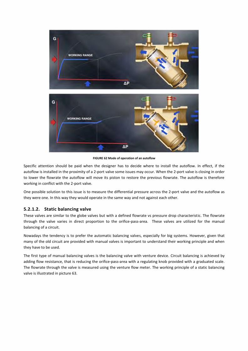
FIGURE 62 Mode of operation of an autoflow
Specific attention should be paid when the designer has to decide where to install the autoflow. In effect, if the
autoflow is installed in the proximity of a 2-port valve some issues may occur. When the 2-port valve is closing in order
to lower the flowrate the autoflow will move its piston to restore the previous flowrate. The autoflow is therefore
working in conflict with the 2-port valve.
One possible solution to this issue is to measure the differential pressure across the 2-port valve and the autoflow as
they were one. In this way they would operate in the same way and not against each other.
5.2.1.2. Static balancing valve These valves are similar to the globe valves but with a defined flowrate vs pressure drop characteristic. The flowrate
through the valve varies in direct proportion to the orifice-pass-area. These valves are utilized for the manual
balancing of a circuit.
Nowadays the tendency is to prefer the automatic balancing valves, especially for big systems. However, given that
many of the old circuit are provided with manual valves is important to understand their working principle and when
they have to be used.
The first type of manual balancing valves is the balancing valve with venture device. Circuit balancing is achieved by
adding flow resistance, that is reducing the orifice-pass-area with a regulating knob provided with a graduated scale.
The flowrate through the valve is measured using the venture flow meter. The working principle of a static balancing
valve is illustrated in picture 63.

58
FIGURE 63 Mode of operation of a manual balancing valve
As we can see, when the flowrate needs to be raised, the knob will be manually rotated in order to extend the orifice-
pass-area, and thus reduce the flow resistance. Conversely, when the flowrate needs to be lowered, the knob will be
manually rotated in the opposite direction, causing the orifice-pass-area to reduce and thus increasing the flowrate.
Usually these valves are mounted on the return branch of the circuit, right after the emitter they have to control.
Another type of static balancing valve is the built-in flowmeter manual valve. The flow meter with magnetic
movement indicator is initially used to set up the reference flowrate. To adjust the flowrate the flow meter control
stem has to be rotated. This will allow the fluid to flow inside the flowmeter and thus to compress the spring. After
the spring has lifted to its maximum value, the ball valve has to be manually rotated to stretch the spring till the value
equivalent to the reference flowrate.
The flowmeter balancing valve and it’s working principle are depicted in figure 64.

FIGURE 64 Working principle of a flowmeter valve: setting the reference flowrate, let the spring lift to its maximum value and finally adjust the
spring position the desired position
This kind of valve is usually applied in the supply branch.
5.2.1.3. Differential pressure control valves Differential pressure control can solve several operating problems in hydronic system, especially in variable flow
systems. The two most common problems are:
- When a control valve is subjected to a too high differential pressure, it cannot shut and may also produce
noise. The differential pressure control can limit the differential pressure to a suitable level;
- When a balancing valve is subjected to large variations in differential pressure, the valve authority may
drop so much that the control became unstable. Differential pressure control can assure that the
authority will remain in an acceptable range.
The differential pressure control valves are used to maintain a constant differential pressure across the valve
regardless the flow rate through it.

60
FIGURE 65 Working principle of a DPCV
To be able to read the pressure in both supply and return pipe a typical dpcv consists of two different bodies, each
one with a regulating knob with a graduated scale, hooked up by an impulse cable. Each body is provided with an
arrow to assure a correct set up. Figure 66 report an illustration of a dpcv.
FIGURE 66 Differential pressure control valve
5.2.2. Hydraulic separator A hydraulic separator is a device that allows separating a circuit in two hydraulically independent sections: the primary
circuit, usually the one with the heat source, and the secondary circuit, usually the one with the loads.
Having to independent circuit will help solving problems regarding variation in circuit pressure and flowrates. To
understand why there might be such issues in a circuit let’s consider the system in figure 67.

FIGURE 67 System with a boiler and three circulating pumps
When the pumps are all turned off there is no pressure difference between the two manifolds.
If the first pump is turned on the pressure difference between the two manifolds will increase. This increase is equal
to the pressure that the pump has to win in order to let the fluid circulate through the boiler. The same increase also
subsists in the crossovers with the pumps turned off, and thus, in the branches number 1 and 2, the fluid might flow in
reverse direction: from the return to the supply manifold.
When the second pump is powered up, to allow the fluid circulate in the right direction, it has first to win the reverse
pressure difference caused by the first pump. Moreover, since it increase the flow rate through the boiler, turning on
the second pump will also increase the pressure difference between the two collectors.
When the last pump is turned on it has to win the reverse pressure created by the other two pumps.
Having high pressure difference between the two manifolds may lead to various issues:
- If there are both little and big pumps installed in the circuit, the little pumps may not be able to
overcome the pressure difference caused by the big pumps. The fluid in their branches will therefore
flow in reverse direction.
- Interferences between non-hydraulically independent circuits may force the pumps to work in non-
design condition, that is with low efficiency and with the possibility to burn the pump.
- If the reverse pressure difference caused by the active pumps is not overcome there may be reverse flow
in the heat emitter. They will be irregularly warmed, causing discomfort in the conditioned environment.
Hydraulic separators can solve all this issues. A system with an installed hydraulic separator is shown in picture 68.

62
FIGURE 68 System with hydraulic separator
In this system the pressure difference between the two manifolds will always be around zero. The explanation is really
simple: the pressure difference between the manifolds is the pressure that the pumps have to overcome to allow the
fluid flowing form the return to the supply manifold. To do that the fluid has to pass through the hydraulic separator,
which is no more than a wide pipe with very low pressure drop. This means that the pumps have to overcome the
pressure drop across the hydraulic separator, which is nearly zero.
In other words, the hydraulic separator creates a zone with a low pressure loss, which enables the primary and
secondary circuit to be hydraulically independent of each other; the flow in one circuit will not create a flow in the
other one.
This means that there will be flow in the secondary circuit only if the pumps are on, permitting the system to meet the
specific requirements at that time. When the pumps are off the whole flowrate will bypass the secondary circuit
through the hydraulic separator. The working principle of a hydraulic separator is shown in figure 69.
FIGURE 69 Three possible working conditions of a hydraulic separator

With a hydraulic separator it is thus possible to have a constant flowrate primary circuit and a variable flowrate
secondary circuit. These operating conditions are nowadays common in both heating and air-conditioning systems.

64
6. PRACTICAL EXAMPLE OF HYDRAULIC BALANCING
6.1. The system In this chapter it will be presented a practical example of hydraulic balancing concerning an existing system. The plant
under consideration is the heating system of a shopping center, provided with 8 fan coil units with a heating power of
6 kW each and 4 door curtain units of 17 kW each. The supply temperature is 70°C and the return temperature is
55°C. The pipes are made of steel, and each emitter involves a pressure drop of 5 kPa. For the pipes a maximum linear
pressure drop of 150 Pa/m has been set. The available balancing valves are STAD, for diameters smaller than 65 cm,
and STAF, for diameters bigger than 65 cm. The model of the shopping center with its heating system is illustrated in
picture 70.
FIGURE 70 Model of the shopping center with his own heating system
6.2. Balancing the system The first step to do is to evaluate the flow rate through the emitters. This can be done with this simple equation:
�̇� = �̇�𝑐𝑝(𝑇𝑖𝑛 − 𝑇𝑜𝑢𝑡)
Where cp is the specific heat of the water (4186,8 J/kg*K), Tin is the supply temperature and Tout is the return
temperature.
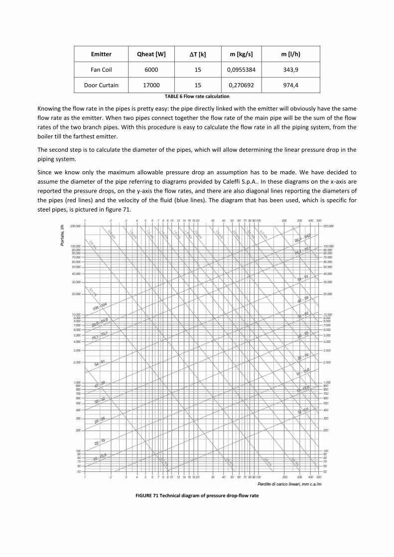
Emitter Qheat [W] T [k] m [kg/s] m [l/h)
Fan Coil 6000 15 0,0955384 343,9
Door Curtain 17000 15 0,270692 974,4
TABLE 6 Flow rate calculation
Knowing the flow rate in the pipes is pretty easy: the pipe directly linked with the emitter will obviously have the same
flow rate as the emitter. When two pipes connect together the flow rate of the main pipe will be the sum of the flow
rates of the two branch pipes. With this procedure is easy to calculate the flow rate in all the piping system, from the
boiler till the farthest emitter.
The second step is to calculate the diameter of the pipes, which will allow determining the linear pressure drop in the
piping system.
Since we know only the maximum allowable pressure drop an assumption has to be made. We have decided to
assume the diameter of the pipe referring to diagrams provided by Caleffi S.p.A.. In these diagrams on the x-axis are
reported the pressure drops, on the y-axis the flow rates, and there are also diagonal lines reporting the diameters of
the pipes (red lines) and the velocity of the fluid (blue lines). The diagram that has been used, which is specific for
steel pipes, is pictured in figure 71.
FIGURE 71 Technical diagram of pressure drop-flow rate

66
The pipeline has been divided in several sections, each of them with his own flow rate. This was necessary since
having different flow rates, even with equal diameters, means having different fluid velocities and thus different linear
pressure drops.
Once the diameter has been set, the fluid velocity can be evaluated knowing that the flow rate can be written as:
�̇� = ∗ 𝑢 ∗ 𝐴
where u is the fluid velocity and A is the pipe section. That equation can also be rewritten making the pipe diameter
explicit:
�̇� = ∗ 𝑢 ∗𝐷2
4
With the fluid velocity the Reynolds number can be estimated. Using the Blasius equation for low surface roughness
will let us calculate the linear pressure drop as:
𝑃𝑙𝑖𝑛 = ∗𝑢2
2∗ 𝑓 ∗
𝐿
𝐷
To calculate the linear pressure drop, the length of the pipe L has been set as 1 m. With these equation the linear
pressure drop (major losses) in Pa/m have been evaluated for all the sections forming the piping system.
Unit m [m3/h] D [m] v [m/s] Re f Pma [Pa/m]
Fan Coil 0,34 0,019 0,337
Door Curtain 0,97 0,025 0,552
O-Boiler 6,65 0,051 0,905 111982 0,017296157 138,77
OP 4,01 0,051 0,546 67575 0,019624093 57,33
PA 3,67 0,051 0,499 61783 0,020068694 49,01
P-FC1 0,34 0,019 0,337 15547 0,02833493 84,75
AB 1,72 0,032 0,594 46156 0,021586327 119,11
BC 1,38 0,032 0,475 36925 0,022824761 80,61
CD 1,03 0,032 0,357 27694 0,024526802 48,72
DE 0,69 0,025 0,389 23632 0,025518859 77,41
B-FC2 0,34 0,019 0,337 15547 0,02833493 84,75
C-FC3 0,34 0,019 0,337 15547 0,02833493 84,75
D-FC4 0,34 0,019 0,337 15547 0,02833493 84,75
E-FC5 0,34 0,019 0,337 15547 0,02833493 84,75
E-FC6 0,34 0,019 0,337 15547 0,02833493 84,75
AX 1,95 0,032 0,673 52310 0,020921332 148,28
X-DC1 0,97 0,025 0,552 33479 0,02339076 142,41
X-DC2 0,97 0,025 0,552 33479 0,02339076 142,41
OQ 2,64 0,039 0,613 58070 0,020382068 98,34
QR 0,69 0,025 0,389 23632 0,025518859 77,41
R-FC7 0,34 0,019 0,337 15547 0,02833493 84,75
R-FC8 0,34 0,019 0,337 15547 0,02833493 84,75
QS 1,95 0,032 0,673 52310 0,020921332 148,28
S-DC3 0,97 0,025 0,552 33479 0,02339076 142,41
S-DC4 0,97 0,025 0,552 33479 0,02339076 142,41 TABLE 7 Major losses calculation, linear major pressure drop
Once the linear pressure drops have been estimated, knowing the length of the pipe from the system sketch, it is
possible to calculate the actual pressure drop per each section of the piping system.

Unit Pma [Pa/m] Lenght [m] Pmaj [kPa]
Fan Coil 84,75
Door Curtain 142,41
O-Boiler 138,77 2,39 0,66
OP 57,33 8,37 0,96
PA 49,01 10,46 1,03
P-FC1 84,75 15,21 2,58
AB 119,11 33,31 7,94
BC 80,61 19,29 3,11
CD 48,72 21,05 2,05
DE 77,41 22,04 3,41
B-FC2 84,75 11,88 2,01
C-FC3 84,75 8,43 1,43
D-FC4 84,75 7,73 1,31
E-FC5 84,75 10,13 1,72
E-FC6 84,75 15,63 2,65
AX 148,28 30,17 8,95
X-DC1 142,41 5,44 1,55
X-DC2 142,41 5,14 1,46
OQ 98,34 28,9 5,68
QR 77,41 13,99 2,17
R-FC7 84,75 7,64 1,29
R-FC8 84,75 27,6 4,68
QS 148,28 26,15 7,76
S-DC3 142,41 2,24 0,64
S-DC4 142,41 6,87 1,96 TABLE 8 Major losses calculation, actual major pressure drop
To evaluate the minor losses the method described by Caleffi has been used. To each emitter has been assigned a
local pressure drop of 5 kPa.

68
Unit v [m/s] Pmin[mm c.a.] Pmin[kPa]
Fan Coil 0,337
Door Curtain 0,552
O-Boiler 0,905 6 241 2,36
OP 0,546 1 16 0,16
PA 0,499 1 12 0,12
P-FC1 0,337 1 7,2 0,07
AB 0,594 2,5 53 0,52
BC 0,475 1 11 0,11
CD 0,357 1 6,4 0,06
DE 0,389 3,5 29 0,28
B-FC2 0,337 1,5 14 0,14
C-FC3 0,337 1,5 14 0,14
D-FC4 0,337 1,5 14 0,14
E-FC5 0,337 1,5 14 0,14
E-FC6 0,337 2,5 17 0,17
AX 0,673 1,5 0,9 0,01
X-DC1 0,552 1,5 31 0,30
X-DC2 0,552 2,5 47 0,46
OQ 0,613 0 0 0,00
QR 0,389 0,5 7,2 0,07
R-FC7 0,337 1 5,7 0,06
R-FC8 0,337 1,5 11 0,11
QS 0,673 1 23 0,23
S-DC3 0,552 1,5 31 0,30
S-DC4 0,552 2,5 47 0,46 TABLE 9 Minor losses calculation
Once both the minor and the major losses are known, the total pressure drops are simply the sum of them.

Unit Pmaj [kPa] Pmin[kPa] Ptot[kPa]
Fan Coil
Door Curtain
O-Boiler 0,66 2,36 3,03
OP 0,96 0,16 1,12
PA 1,03 0,12 1,14
P-FC1 2,58 0,07 7,65
AB 7,94 0,52 8,46
BC 3,11 0,11 3,22
CD 2,05 0,06 2,11
DE 3,41 0,28 3,70
B-FC2 2,01 0,14 7,15
C-FC3 1,43 0,14 6,57
D-FC4 1,31 0,14 6,45
E-FC5 1,72 0,14 6,85
E-FC6 2,65 0,17 7,82
AX 8,95 0,01 8,96
X-DC1 1,55 0,30 6,85
X-DC2 1,46 0,46 6,92
OQ 5,68 0,00 5,68
QR 2,17 0,07 2,24
R-FC7 1,29 0,06 6,35
R-FC8 4,68 0,11 9,79
QS 7,76 0,23 7,98
S-DC3 0,64 0,30 5,94
S-DC4 1,96 0,46 7,42 TABLE 10 Total pressure drops calculation
The goal of this procedure is to find the most unfortunate emitter. It will be that emitter that involves the greatest
pressure drop between itself and the boiler. The head pump will be equal to this pressure drop. Therefore, for each
emitter, we have to sum the total pressure drop of those sections that connect that emitter to the boiler.
Unit P [kPa]
Fan Coil 1 11,79
Fan Coil 2 20,89
Fan Coil 3 23,53
Fan Coil 4 25,52
Fan Coil 5 29,63
Fan Coil 6 35,99
Fan Coil 7 17,30
Fan Coil 8 20,73
Door Curtain 1 24,05
Door Curtain 2 21,17
Door Curtain 3 22,63
Door Curtain 4 24,11 TABLE 11 Pressure drop between emitters and boiler
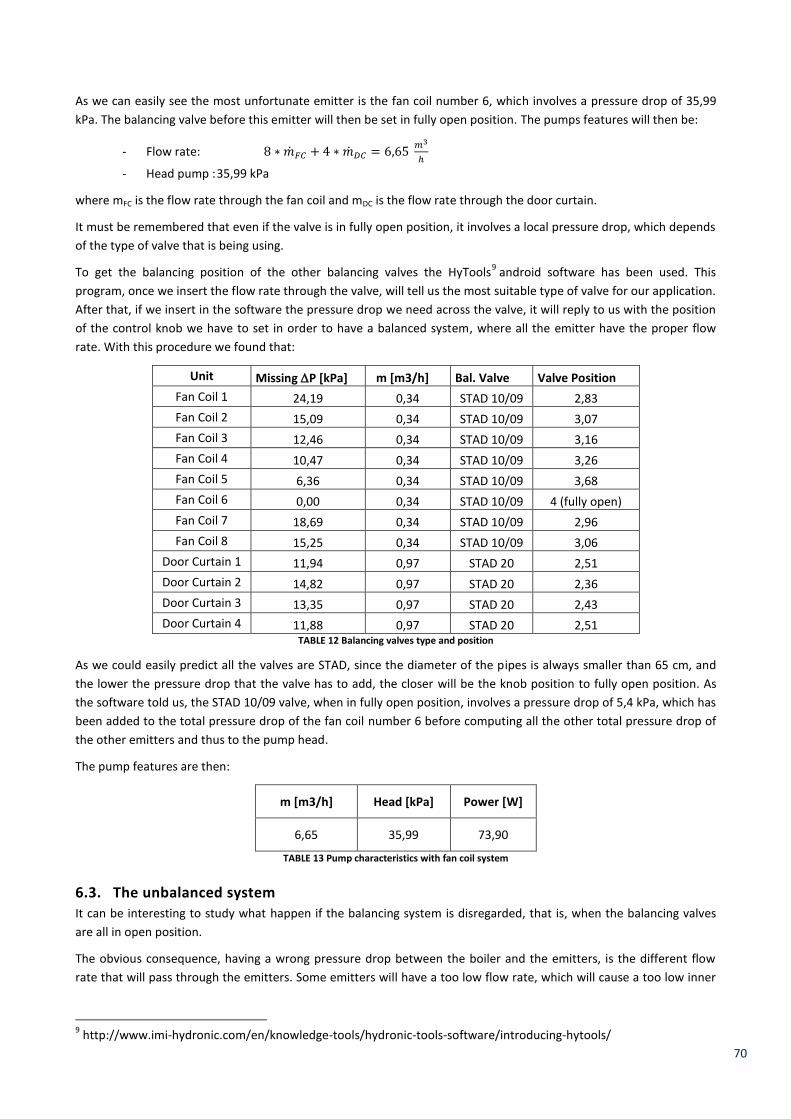
70
As we can easily see the most unfortunate emitter is the fan coil number 6, which involves a pressure drop of 35,99
kPa. The balancing valve before this emitter will then be set in fully open position. The pumps features will then be:
- Flow rate: 8 ∗ �̇�𝐹𝐶 + 4 ∗ �̇�𝐷𝐶 = 6,65 𝑚3
ℎ
- Head pump : 35,99 kPa
where mFC is the flow rate through the fan coil and mDC is the flow rate through the door curtain.
It must be remembered that even if the valve is in fully open position, it involves a local pressure drop, which depends
of the type of valve that is being using.
To get the balancing position of the other balancing valves the HyTools9 android software has been used. This
program, once we insert the flow rate through the valve, will tell us the most suitable type of valve for our application.
After that, if we insert in the software the pressure drop we need across the valve, it will reply to us with the position
of the control knob we have to set in order to have a balanced system, where all the emitter have the proper flow
rate. With this procedure we found that:
Unit Missing P [kPa] m [m3/h] Bal. Valve Valve Position
Fan Coil 1 24,19 0,34 STAD 10/09 2,83
Fan Coil 2 15,09 0,34 STAD 10/09 3,07
Fan Coil 3 12,46 0,34 STAD 10/09 3,16
Fan Coil 4 10,47 0,34 STAD 10/09 3,26
Fan Coil 5 6,36 0,34 STAD 10/09 3,68
Fan Coil 6 0,00 0,34 STAD 10/09 4 (fully open)
Fan Coil 7 18,69 0,34 STAD 10/09 2,96
Fan Coil 8 15,25 0,34 STAD 10/09 3,06
Door Curtain 1 11,94 0,97 STAD 20 2,51
Door Curtain 2 14,82 0,97 STAD 20 2,36
Door Curtain 3 13,35 0,97 STAD 20 2,43
Door Curtain 4 11,88 0,97 STAD 20 2,51 TABLE 12 Balancing valves type and position
As we could easily predict all the valves are STAD, since the diameter of the pipes is always smaller than 65 cm, and
the lower the pressure drop that the valve has to add, the closer will be the knob position to fully open position. As
the software told us, the STAD 10/09 valve, when in fully open position, involves a pressure drop of 5,4 kPa, which has
been added to the total pressure drop of the fan coil number 6 before computing all the other total pressure drop of
the other emitters and thus to the pump head.
The pump features are then:
m [m3/h] Head [kPa] Power [W]
6,65 35,99 73,90
TABLE 13 Pump characteristics with fan coil system
6.3. The unbalanced system It can be interesting to study what happen if the balancing system is disregarded, that is, when the balancing valves
are all in open position.
The obvious consequence, having a wrong pressure drop between the boiler and the emitters, is the different flow
rate that will pass through the emitters. Some emitters will have a too low flow rate, which will cause a too low inner
9 http://www.imi-hydronic.com/en/knowledge-tools/hydronic-tools-software/introducing-hytools/

temperature. Conversely some other emitters will have a too high flow rate, which will cause a too high inner
temperature.
It must always be remembered that the radiator characteristic is not linear, thus, the effect on the inner temperature
of a too high and of a too low flow rate will not be of the same amount.
The correct procedure to follow would be an iterative calculation, since to know the new flow rate through the
emitters we have to know the new pressure drop in the pipes, which depends on the velocity of the fluid, which in
turn depends on the flow rate.
In order to make the calculation easier we will use some approximations. First of all we consider that the flow rate at
the pumps remains constant, which is obviously not true since having all the balancing valves in fully open position
means that there will be a different pressure drop among the pipes (lower) and thus a different system characteristic,
so the duty point, and the flow rate with it, will change.
The second approximation is that the pressure drop among the pipes doesn’t change with the flow rate: this allows us
to compare the piping system before and after the valves opening, and lets us calculate the new flow rate though the
pipes.
The starting point will be the pump, of which we know the flow rate thanks to previous calculations.
�̇�𝑝𝑢𝑚𝑝 = 6,65 𝑚3
ℎ
The second step is to consider the first branch point after the pump where the flow rate splits up into two. We know
that the sum of the two branches flow rate is equal to the pump flow rate.
�̇�𝑏𝑟𝑎𝑛𝑐ℎ1 + �̇�𝑏𝑟𝑎𝑛𝑐ℎ2 = �̇�𝑝𝑢𝑚𝑝
Per each branch we also know the pressure drop, thanks to our second approximation, and the flow rate through it
when the valves were in the working position. Knowing that the pressure drop is a square function of the flow rate
and that the branch with the lower pressure drop will have the major flow rate we can also write that:
𝐻𝑏𝑟𝑎𝑛𝑐ℎ1
𝐻𝑏𝑟𝑎𝑛𝑐ℎ2
= (�̇�𝑏𝑟𝑎𝑛𝑐ℎ2
�̇�𝑏𝑟𝑎𝑛𝑐ℎ1
)
2
Repeating this simple procedure for all branch points in the piping system will be possible to calculate the flow rate
through all the emitters. The final results are shown in table 13.
Unit Prev. flow rate
[m3/h]
New flow rate [m
3/h]
Gain-Loss [m
3/h]
FC1 0,34 1,864 1,524
FC2 0,34 0,295 -0,044
FC3 0,34 0,134 -0,206
FC4 0,34 0,060 -0,280
FC5 0,34 0,026 -0,314
FC6 0,34 0,025 -0,315
FC7 0,34 0,948 0,608
FC8 0,34 0,849 0,509
DC1 0,97 0,341 -0,628
DC2 0,97 0,341 -0,629
DC3 0,97 0,901 -0,069
DC4 0,97 0,864 -0,106 TABLE 14 Results of unbalanced system on the flow rate
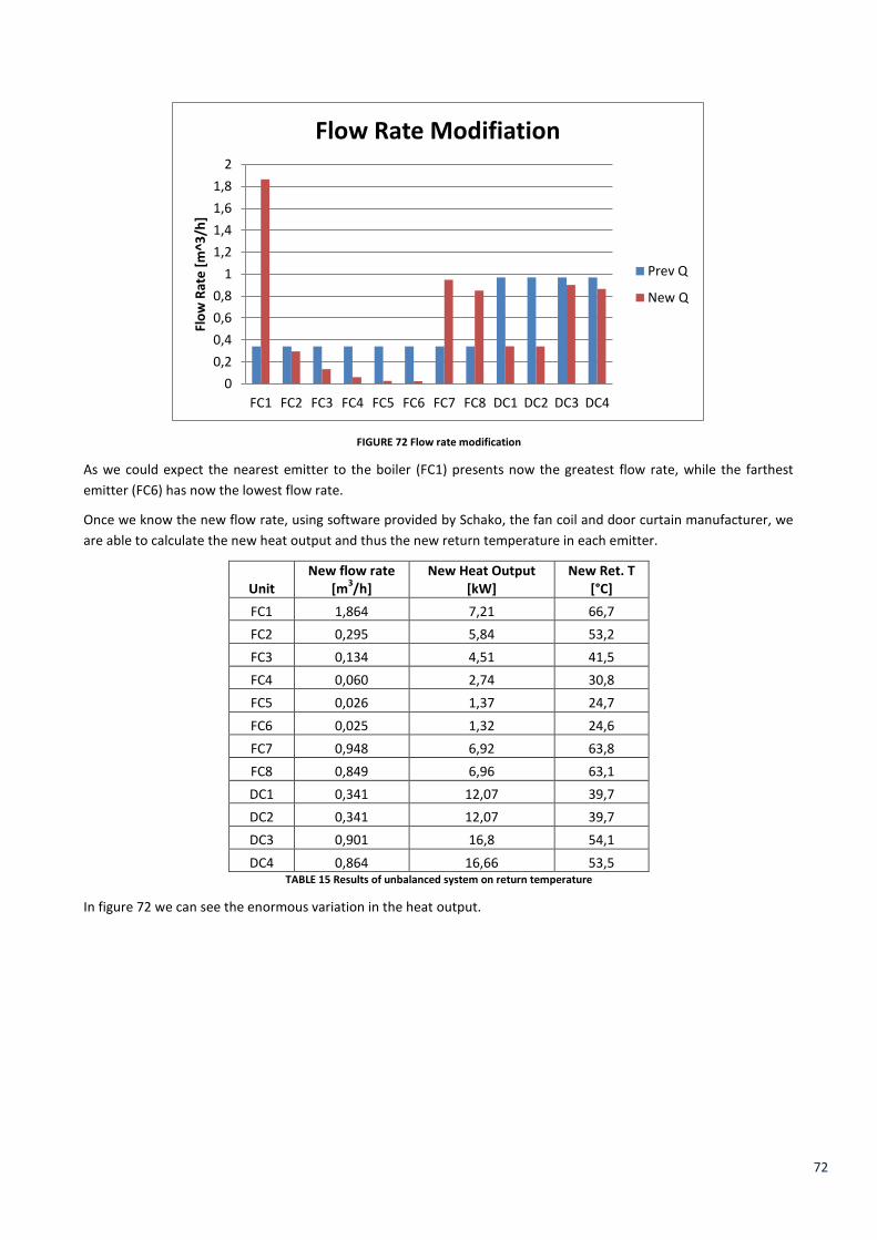
72
FIGURE 72 Flow rate modification
As we could expect the nearest emitter to the boiler (FC1) presents now the greatest flow rate, while the farthest
emitter (FC6) has now the lowest flow rate.
Once we know the new flow rate, using software provided by Schako, the fan coil and door curtain manufacturer, we
are able to calculate the new heat output and thus the new return temperature in each emitter.
Unit New flow rate
[m3/h]
New Heat Output [kW]
New Ret. T [°C]
FC1 1,864 7,21 66,7
FC2 0,295 5,84 53,2
FC3 0,134 4,51 41,5
FC4 0,060 2,74 30,8
FC5 0,026 1,37 24,7
FC6 0,025 1,32 24,6
FC7 0,948 6,92 63,8
FC8 0,849 6,96 63,1
DC1 0,341 12,07 39,7
DC2 0,341 12,07 39,7
DC3 0,901 16,8 54,1
DC4 0,864 16,66 53,5 TABLE 15 Results of unbalanced system on return temperature
In figure 72 we can see the enormous variation in the heat output.
0
0,2
0,4
0,6
0,8
1
1,2
1,4
1,6
1,8
2
FC1 FC2 FC3 FC4 FC5 FC6 FC7 FC8 DC1 DC2 DC3 DC4
Flo
w R
ate
[m
^3/h
]
Flow Rate Modifiation
Prev Q
New Q

FIGURE 73Heat output modification
The software bases its calculation on three equations. The first one is the heat carrier cooling in the terminal:
𝑄 = �̇�𝑐𝑝(𝑇𝑖𝑛 − 𝑇𝑜𝑢𝑡)
where Tin and Tout are respectively the inlet and exit fluid temperature in the emitter. The second equation is the heat
transfer equation between the heat carrier and the room air:
𝑄 = 𝐾𝐴𝑇𝑚𝑙
where the mean logarithmical temperature difference Tml is:
𝑇𝑚𝑙 =𝑇𝑖𝑛 − 𝑇𝑜𝑢𝑡
ln (𝑇𝑖𝑛 − 𝑇𝑖
𝑇𝑜𝑢𝑡 − 𝑇𝑖)
where Ti is the inner room temperature. The last equation is the heat loss equation for the room:
𝑄 = ∑ 𝑈𝐴(𝑇𝑖 − 𝑇𝑒) + ∑ 𝑙(𝑇𝑖 − 𝑇𝑒) + 𝑉 ∗ 𝑛 ∗ 𝑐𝑝𝑎𝑖𝑟
𝑎𝑖𝑟(𝑇𝑖 − 𝑇𝑒)
where Te is the outside temperature. The first term is the heat exchange between the walls and the outside air, the
second one is the heat transfer due to thermal bridges and the last one is the heat loss due to air currents coming into
the room from the outside environment.
The system based on these three equations can be solved only by iterative methods. The equations are in effect
influenced by these three parameters:
- The return temperature of central heating system, which affects the first and second equations;
- The indoor temperature, which affects the second and the third equations;
- The mass flow, which affects the second equation.
As we expected, both the heat output and the return temperature rise in those emitters where the flow rate have had
a boost. While the boost in the heat output can be explained with the increasing heat exchange factor, the boost in
the return temperature is due to the less time that the single water particles spend inside the emitter.
0
2
4
6
8
10
12
14
16
18
FC1 FC2 FC3 FC4 FC5 FC6 FC7 FC8 DC1 DC2 DC3 DC4
Hea
t O
utp
ut
[kW
]
Heat Output Modification
Previous Q
New Q

74
7. UNDERFLOOR HEATING SYSTEM
In this last chapter the entire heating system will be substituted by an underfloor heating system. Only the door
curtains will not be modified. The goal is to compare the two different systems and to determine which one involves
bigger electricity consumption and bigger boiler generation performance.
7.1. Design of the underfloor heating system To make a fair comparison we will consider the same total heating power used for the fan coils, that is 48 kW. Since 48
kW are not enough to heat up all the surface of the mall we’ll consider only a part of the floor, which will allow us to
have a specific heating power around 40 kW/m2, which is the typical power range for this kind of heating systems.
The typical equation for an underfloor heating system specific power is:
𝑞 = 𝐾ℎℎ
where the unit of measure of q is W/m2, Kh is the heat exchange coefficient, usually provided by the system
manufacturer, and h is a logarithmic temperature difference. Since we were not in contact with a manufacturer the
value of Kh has been supposed.
Qtot [W] Area [m^2] Qspec [W/m^2] Kh [W/K*m^2] h [K]
48000,00 1152,90 41,63 3,90 10,68
TABLE 16 Underfloor heating system specific power
Knowing the Kh allows us to calculate the average water temperature in the underfloor circuits:
𝑤̅̅ ̅̅ = 𝑖 + ℎ
where i is the inner room temperature.
A typical underfloor heating system has a temperature difference between the supply and the return of 5 or 6
degrees, this value is known as σ. If we set this value we can calculate the supply (v) and return temperature (r)
using the average water temperature w. The σ value has been set to 6.
𝑣 = 𝑤̅̅ ̅̅ +
𝜎
2
𝑟 = 𝑤̅̅ ̅̅ −
𝜎
2
Knowing the temperature difference is then easy to calculate the total mass flow rate in the system.
h [°C] w [°C] v [°C] r [°C] m [kg/s] m [l/h]
10,68 28,68 31,68 25,68 1,91 6878,76
TABLE 17 Supply and return temperature calculation
The next step is to calculate the portion of floor that will be occupied by each underfloor circuit. To do so we need the
specs of the pipes that will be placed underfloor. We have considered a PEX tube with 20 mm of external diameter
and 16 mm of internal diameter. The pitch between the tubes is 15 mm. These data can be used in a diagram, as the
one showed in figure 72, to calculate the maximum allowable mass flow per circuit, once we have set the allowable
pressure loss per meter. In this case we will assume a linear pressure loss of 10 mmH20/m.

FIGURE 74 Pressure loss in PEX tube
As shown in the diagram, the maximum allowable mass flow rate per each circuit is around 230 l/h. To calculate the
length of each circuit we have to set the maximum permissible pressure loss that each circuit must not overtake,
which will be 1 mH20.
The length of each circuit will then be:
𝐿 =1 𝑚𝐻20
10 𝑚𝑚𝐻20
𝑚
= 100 𝑚
The area occupied by each circuit can be calculated knowing the pitch between each tube:
𝐴 = 𝐿𝑒𝑛𝑔ℎ𝑡 ∗ 𝑝𝑖𝑡𝑐ℎ = 100 ∗ 0,015 = 15 𝑚2
The number of circuits we will have to use is:
𝑁𝑐 =𝑇𝑜𝑡𝑎𝑙 𝑓𝑙𝑜𝑜𝑟 𝑎𝑟𝑒𝑎
𝐶𝑖𝑟𝑐𝑢𝑖𝑡 𝑎𝑟𝑒𝑎=
1152,9
15= 76,86
Since each manifold is connected to 6 circuits at the same time we will use 12 manifolds connected to 72 circuits in
total.
We now have to calculate the pressure loss per each manifold. The pressure loss that involves a manifold, as shown in
picture 73, is composed by different terms.

76
FIGURE 75Manifold pressure drops
From the supply to the return side we have:
- Pvs: pressure loss in the globe sphere valve;
- PcollM: pressure loss in the supply manifold;
- Pvr: pressure loss in the regulation valve;
- Panello: pressure loss in the underfloor circuit;
- Pvi: pressure loss in the interception valve;
- PcollR: pressure loss in the return manifold.
The pressure drops have been evaluated with this equation:
𝑃 =�̇�2
𝐾𝑣2
where Kv represents the mass flow rate through the device which causes a pressure drop of 1 kPa. This value is
provided by the manufacturer of the manifold. Per each manifold we thus find that the pressure drop is 12,74 kPa.
Gtot [l/h] 573,23
P_circ [kPa] 10,00
P_vr [kPa] 1,55
P_vi [kPa] 0,85
P_coll_M [kPa] 0,17
P_coll_R [kPa] 0,17
P_vs [kPa] 0,01
TABLE 18Manifold pressure drop calculation
We now have to evaluate the pressure drop between the manifold and the boiler. This is necessary to calculate the
head of the circuit pump. To do so a sketch of the system has been drawn, that is represented in picture 74. This is not
the only way to design the plant, it has been chosen due to its simplicity.

FIGURE 76 Sketch of the underfloor heating circuit piping system
With this scheme we can now calculate the pressure drop of the most unfortunate manifold in the same way we have
previously calculated the pressure drop for the most unfortunate emitter. The final results are:
Unit P [kPa]
M1 16,46
M2 23,18
M3 30,58
M4 35,02
M5 35,76
M6 37,55
M7 16,36
M8 17,19
M9 23,83
FIGURE 77 Manifold total pressure drops
The most unfortunate manifold is the farthest manifold, the number 6, which is the one in the bottom left corner of
the area.
In this case, the pump features are:
�̇� [m3/h] Head [kPa] Power [W]
6,88 37,55 79,77
TABLE 19 Pump characteristics with underfloor heating system

78
8. COMPARISON BETWEEN FAN COIL SYSTEM AND UNDERFLOOR HEATING SYSTEM
In this last chapter we will compare the two heating system that have been discussed in the previous chapters. To do
so we need a parameter we can use to compare the two systems. This parameter is the load factor Fc. The load factor
is the ratio between the difference of the average internal and external temperature (which represents, when
multiplied for the days in a month, the degrees day) and the difference of design internal and external temperature.
𝐹𝑐 =�̅�𝑒𝑠𝑡 − 𝑇𝑖𝑛𝑡
𝑇𝑑𝑒𝑠,𝑒𝑠𝑡 − 𝑇𝑖𝑛𝑡
Since we had no access to the Hungarian UNI EN standards we referred to the website woitalia.it where daily average
temperature can be found from 1980 till today. Using the data from this website we can calculate the daily monthly
average temperature per each month as the mean between maximum and minimum daily temperature.
The design internal temperature has been set to 18 °C, while the design external temperature to -10°C. These two
values have been chosen referring to personal experience and not to a standard because we had no access to it.
The calculation of the load factor is depicted in table 20.
Month Tmax [°C] Tmin [°C] Tav [°C] DD Tdesign_est
[°C] FC Working hours
Jen 2,10 -4,60 -1,25 578 -10 0,69 288,75
Feb 4,30 -2,80 0,75 518 -10 0,62 258,75
Mar 10,50 1,20 5,85 365 -10 0,43 182,25
Apr 17,30 6,30 11,80 186 -10 0,22 93,00
May 22,20 11,00 16,60 42 -10 0,05 21,00
Jun 25,40 14,40 19,90 -57 -10 -0,07 -28,50
Jul 27,50 16,20 21,85 -116 -10 -0,14 -57,75
Aug 27,40 15,60 21,50 -105 -10 -0,13 -52,50
Sep 22,00 11,20 16,60 42 -10 0,05 21,00
Oct 16,20 0,63 8,42 288 -10 0,34 143,78
Nov 9,30 1,70 5,50 375 -10 0,45 187,50
Dec 2,60 -3,20 -0,30 549 -10 0,65 274,50
TABLE 20 Load factor and working hours
The load factor is used to calculate the number of hour per month that the system, thus the pump, has to work. It’s
referred to a normal shift, which begins at 8 am and ends at 10 pm. This means that, to calculate the working hours of
the pump we have to multiply the standard shift (14 hours) and the load factor.
The total working hour, considering a heating season, which start in October and ends in April, is 1429. We now can
calculate the energy absorption of the pump in the two different systems, which will be the product between the
pump power and the working hours.
System P [kW] H [h] E [kWh]
FanCoil 0,07 1428,53 105,57
Uderfloor 0,06 1428,53 86,37
TABLE 21 Pumps electrical absorption
As we can see the electrical absorption in the two cases is not so different and in both cases is quite low. The reason is
the little power of the plant, just 48 kW.

9. CONCLUSION
In this thesis we have tried to explain why and how a system should be properly balanced. As we have seen, an
improper balancing would lead to uncomfortable environment conditions, such as wrong inner temperature,
disturbing flow rates through valves and pipes and excessive power consumption due to incorrect flow rates.
A correct balancing procedure starts from the design of the heating/cooling plant and not when the system is already
placed. This allows the designer to make the best choices in order to save money thanks to a correct piping and pump
design, to get a performing plant and to respect the environment standard policy. Since the balancing procedure itself
is not so complicate and all in all quite precise, although it is based on approximations, in my opinion it should be
made compulsory for every new system.
Thanks to the practical example, even though is a simplified model on a very simple heating system, is clear how much
the performance of our plant, therefore the quality of the environment, is greatly influenced by the correct or wrong
balancing of the heating system: the heat output of the fan coil changes from +21% (FC1) to -340% (FC6).
If we really want to elevate the standards of quality living in our houses and inner environment, the hydraulic
balancing of the heating/cooling plants cannot be neglected.
With regard to the two systems comparison, even though this is a very simplified case, the fan coil, as expected,
shows a greater electrical assumption due to a bigger pump power. It can be also explained analyzing the piping
system served by the pump. In the fan coil case the pump supplies both the fan coils and the door curtains, while in
the underfloor heating system the door curtains have a separate circulating pump.

80
Bibliography
- Alameddine F., Gunnarson A., An Engineer’s Guide for Sizing and Specifying Pressure Indipendent Control
Valves for Building Services, FlowLine Controls, 2008
- Autoflow Automatic Balancing, FDI Flow Design INC, 2007
- Boysen H., kv: what, why, how, whence?, Danfoss Thecnical Paper, 2011
- Eisenberg P., Cavitation, Hydronautics Incorporated
- Goodwill I.M., Sleigh P.A., Fluid Flow in Pipes, CIVE2400 Fluid Mechanics, January 2008
- Grundfos Handbook, Pump Handbook, Grundfos, 2004
- Huebsch W., Munson R., Okiishi H., Young F., Fundamentals of Fluid Mechanics Sixth edition, United State
of America, Wiley, 2009
- Kiijarvi J.,Darcy friction factor formulae in turbulent pipe flow, Lunowa Fluid Mechanics Paper, 2011
- KSB Know-how Volume 4, Pump Control/System Automation, August 2006
- Siegenthaler J., Back to Basics: Reversing Course, January 1, 2007
- Siemens, Hydraulic in Building Systems, Siemens Building Technologies
- Sleigh A., An Introduction to Fluid Mechanics, University of Leeds, 2001
- Warburton P., Building Control System, CIBSE Guide, February 2009
- http://www.engineeringtoolbox.com/
- http://www.spiraxsarco.com/
- http://www.caleffi.com
- http://www.woitalia.it