hyderabad, india, 2010 an exercise in mirror symmetry
TRANSCRIPT

Proceedings of the International Congress of MathematiciansHyderabad, India, 2010
An exercise in mirror symmetry
Richard P. Thomas
Abstract. This expository article is an attempt to illustrate the power of Kontsevich’shomological mirror symmetry conjecture through one example, the heuristics of whichlead to an algebro-geometric construction of knot invariants.
Mathematics Subject Classification (2010). Primary 14J33; Secondary 53D37,
57M27, 53C26.
Keywords. Mirror symmetry, Khovanov cohomology.
1. Introduction
This paper can be thought of as a companion to the paper [32], giving the back-ground, mirror symmetric motivation, and helpful pictures that are missing there.Along the way we give a geometric description of Manolescu’s isomorphism [18]between an open subset of a Hilbert scheme of points on an ALE space and theSlodowy slice to a nilpotent matrix with two equal Jordan blocks considered bySeidel and Smith, along the lines of the construction in [11]. We use a descriptionof these ALE spaces as blow ups which is probably well known to experts but wasnew to me, giving maps between them that are crucial to our construction.Heuristics. We treat mirror symmetry as a heuristic device to motivate con-structions on one side of the mirror that reflect better known constructions on theother. We make no rigorous claims for our putative mirrors; for instance we are notclaiming that a hyperkahler resolution of a singularity is mirror to a hyperkahlersmoothing. Though we will use examples where this ansatz works well, in the keyexample it fails (see Section 5.1) and has to be augmented with a deformation.Acknowledgements. I would like to thank Gordon Brown, Chris Murphy, WilsonSutherland, Simon Donaldson, Paul Seidel, Mikhail Khovanov, Shing-Tung Yau,Daniel Huybrechts, Tom Bridgeland and Rahul Pandharipande for educating me,and my collaborator Ivan Smith with whom much of this work was done. Thanksalso to Arthur Greenspoon and Ivan Smith for carefully reading the manuscript.
2. Symplectic geometry
We begin by surveying some standard constructions in symplectic geometry. Weskate over many technical issues, in particular Floer cohomology, gradings, the

2 Richard P. Thomas
construction of the Fukaya category, and the difficulties in doing symplectic paralleltransport in noncompact spaces. Most of these are dealt with manfully in thewonderful papers of Paul Seidel [23, 24, 25].
2.1. Parallel transport. A family of projective manifolds
p : X → B
will not in general be locally trivial over its smooth locus B∗ ⊂ B; the complexstructure will vary. As Paul Seidel once taught me, symplectic geometry is whatis left when you look for what is locally constant. (I liked this because it soundedlike it might subordinate symplectic geometry to algebraic geometry.) Here thesymplectic form ω is given by pulling back the Fubini-Study form via a projectiveembedding. Over B∗ there is a connection on the family: take the annihilatorof the fibrewise tangent bundle TX/B under ω to define the horizontal subbundleof TX . Parallel transport along this connection preserves the symplectic form,and so identifies smooth fibres Xb0 , Xb1 by symplectomorphisms, once we pick apath between their images b0, b1 in the base B
∗. In particular the monodromyaround a loop in B∗ can be taken to be a symplectomorphism of any such fibre(X,ω) ∼= (Xb, ω|Xb).This connection is not flat. Any two tangent vectors v1, v2 ∈ TbB∗ have unique
horizontal lifts vi ∈ Γ(TX |Xb). Thinking of
h := ω(v1, v2)
as a Hamiltonian function on Xb it defines an infinitesimal symplectomorphism ofXb by the Hamiltonian vector field Xh whose contraction with ω|Xb is dh. ThisHam(Xb, ω|Xb)-valued 2-form on B
∗ is the curvature of the connection. Thereforeisotopic loops in B∗ give rise to different but Hamiltonian isotopic monodromies.We get a homomorphism
π1(B∗)→ Aut(X,ω)
to the group of symplectomorphisms modulo Hamiltonian isotopies.Pick a singular point x0 lying above a point b0 ∈ B in the discriminant locus,
and a path in B∗ to b ∈ B∗. The locus L of points of Xb that flow to x0 byparallel transport along the path is called the vanishing cycle of the singularityx0. Because the flow preserves the symplectic structure, L is isotropic (where it issmooth): ω|TL ≡ 0. If x0 is an isolated critical point then L is in fact Lagrangian.The curvature of the symplectic connection blows up as we approach such
singular points. Taking smaller and smaller loops in B∗ around b0 the monodromysymplectomorphism approaches the identity away from the vanishing cycle.
2.2. The ordinary double point. We start with a basic affine localmodel. Consider the family
f : Cn+1 −→ C, f(x) =n+1∑
i=1
x2i . (2.1)

An exercise in mirror symmetry 3
Figure 1. Vanishing cycle L of the family (2.1).
Over 0 we get the n-dimensional ordinary double point∑x2i = 0, while over ε 6= 0
we find its smoothing Xε = {∑x2i = ε}. We use the symplectic structure inherited
from the standard Kahler form on Cn+1.Using the O(n+ 1) symmetry it is easy to see that the vanishing cycle L over
ε 6= 0 along the straight line path to 0 ∈ C is the real slice
xi ∈√ε.R ⊂ C
of X. Scaling coordinates by ε−1/2 this is just the sphere
L = Sn ={∑
x2i = 1}⊂ Rn+1.
In fact take ε ∈ (0,∞), without loss of generality, and take real and imaginaryparts: xj = aj + ibj . Consider a = (ai) and b = (bi) as lying in Rn+1 and (Rn+1)∗
respectively, and give Cn+1 = Rn+1 ⊕ (Rn+1)∗ = T ∗Rn+1 its canonical symplecticstructure. Then the equation f = ε becomes
∑a2i − b
2i = ε,
∑aibi = 0.
In particular |a|2 = ε+ |b|2 > 0 so we may divide a and multiply b by |a| to givea symplectomorphism of f−1(ε) to
T ∗Sn = {(a,b) ∈ T ∗Rn+1 : |a| = 1, b(a) = 0}.
The monodromy on going once anticlockwise around ε = 0 is Seidel’s generalisedDehn twist TL [22] about L (first suggested by Arnol’d). This is (Hamiltonianisotopic to) the time π flow by the Hamiltonian φ(|b|), where φ is a smooth mono-tonic function with φ(x) = x for small x ≥ 0 and φ ≡ const for large x. This flowis discontinuous across the vanishing cycle b = 0, but after time π comes back tothe antipodal map there and so becomes continuous again. (Alternatively use thestandard metric to identify T ∗Sn with TSn. The latter has a canonical vector fieldwhich at a point v ∈ TpSn is the horizontal lift v of v to T(p,v)(TSn). Flowing downv/|v| is again discontinuous, cutting T ∗Sn along its zero section then regluing aftertime π. Then use a bump function to glue this symplectomorphism to the identityaway from the zero section.)
4 Richard P. Thomas
When n = 1 this reduces to the classical Dehn twist along an embedded S1
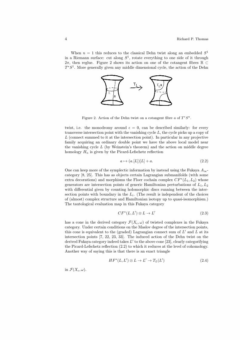
in a Riemann surface: cut along S1, rotate everything to one side of it through2π, then reglue. Figure 2 shows its action on one of the cotangent fibres R ⊂T ∗S1. More generally given any middle dimensional cycle, the action of the Dehn
Figure 2. Action of the Dehn twist on a cotangent fibre a of T ∗Sn.
twist, i.e. the monodromy around ε = 0, can be described similarly: for everytransverse intersection point with the vanishing cycle L, the cycle picks up a copy ofL (connect summed to it at the intersection point). In particular in any projectivefamily acquiring an ordinary double point we have the above local model nearthe vanishing cycle L (by Weinstein’s theorem) and the action on middle degreehomology Hn is given by the Picard-Lefschetz reflection
a 7→ (a.[L])[L] + a. (2.2)
One can keep more of the symplectic information by instead using the Fukaya A∞-category [8, 25]. This has as objects certain Lagrangian submanifolds (with someextra decorations) and morphisms the Floer cochain complex CF ∗(L1, L2) whosegenerators are intersection points of generic Hamiltonian perturbations of L1, L2with differential given by counting holomorphic discs running between the inter-section points with boundary in the Li. (The result is independent of the choicesof (almost) complex structure and Hamiltonian isotopy up to quasi-isomorphism.)The tautological evaluation map in this Fukaya category
CF ∗(L,L′)⊗ L→ L′ (2.3)
has a cone in the derived category F(Xε, ω) of twisted complexes in the Fukayacategory. Under certain conditions on the Maslov degree of the intersection points,this cone is equivalent to the (graded) Lagrangian connect sum of L′ and L at itsintersection points [7, 22, 23, 33]. The induced action of the Dehn twist on thederived Fukaya category indeed takes L′ to the above cone [23], clearly categorifyingthe Picard-Lefschetz reflection (2.2) to which it reduces at the level of cohomology.Another way of saying this is that there is an exact triangle
HF ∗(L,L′)⊗ L→ L′ → TL(L′) (2.4)
in F(Xε, ω).
An exercise in mirror symmetry 5
2.3. Families of quadrics. Another way of seeing the smoothing of theordinary double point – i.e. a smooth fibre of (2.1) – is by fibring it over C usingthe last coordinate xn+1 = t:
{n∑
i=1
x2i = ε− t2
}
⊂ Cnxi × Ct −→ Ct. (2.5)
This expresses the n-dimensional affine quadric as a family of (n− 1)-dimensionalaffine quadrics – the fibres
∑ni=1 x
2i =const where t is fixed. Each contains a
canonical Lagrangian Sn−1 real slice, except the two singular fibres where ε − t2
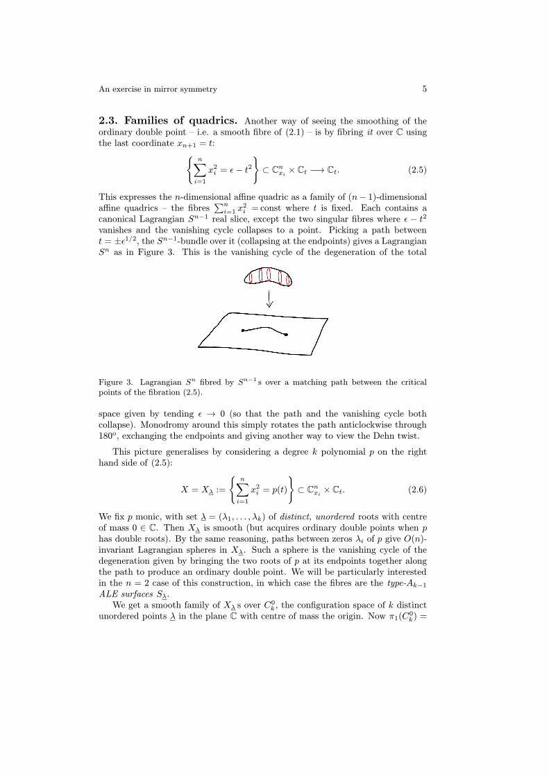
vanishes and the vanishing cycle collapses to a point. Picking a path betweent = ±ε1/2, the Sn−1-bundle over it (collapsing at the endpoints) gives a LagrangianSn as in Figure 3. This is the vanishing cycle of the degeneration of the total
Figure 3. Lagrangian Sn fibred by Sn−1 s over a matching path between the criticalpoints of the fibration (2.5).
space given by tending ε → 0 (so that the path and the vanishing cycle bothcollapse). Monodromy around this simply rotates the path anticlockwise through180o, exchanging the endpoints and giving another way to view the Dehn twist.
This picture generalises by considering a degree k polynomial p on the righthand side of (2.5):
X = Xλ :=
{n∑
i=1
x2i = p(t)
}
⊂ Cnxi × Ct. (2.6)
We fix p monic, with set λ = (λ1, . . . , λk) of distinct, unordered roots with centreof mass 0 ∈ C. Then Xλ is smooth (but acquires ordinary double points when phas double roots). By the same reasoning, paths between zeros λi of p give O(n)-invariant Lagrangian spheres in Xλ. Such a sphere is the vanishing cycle of thedegeneration given by bringing the two roots of p at its endpoints together alongthe path to produce an ordinary double point. We will be particularly interestedin the n = 2 case of this construction, in which case the fibres are the type-Ak−1ALE surfaces Sλ.We get a smooth family of Xλ s over C
0k , the configuration space of k distinct
unordered points λ in the plane C with centre of mass the origin. Now π1(C0k) =
6 Richard P. Thomas
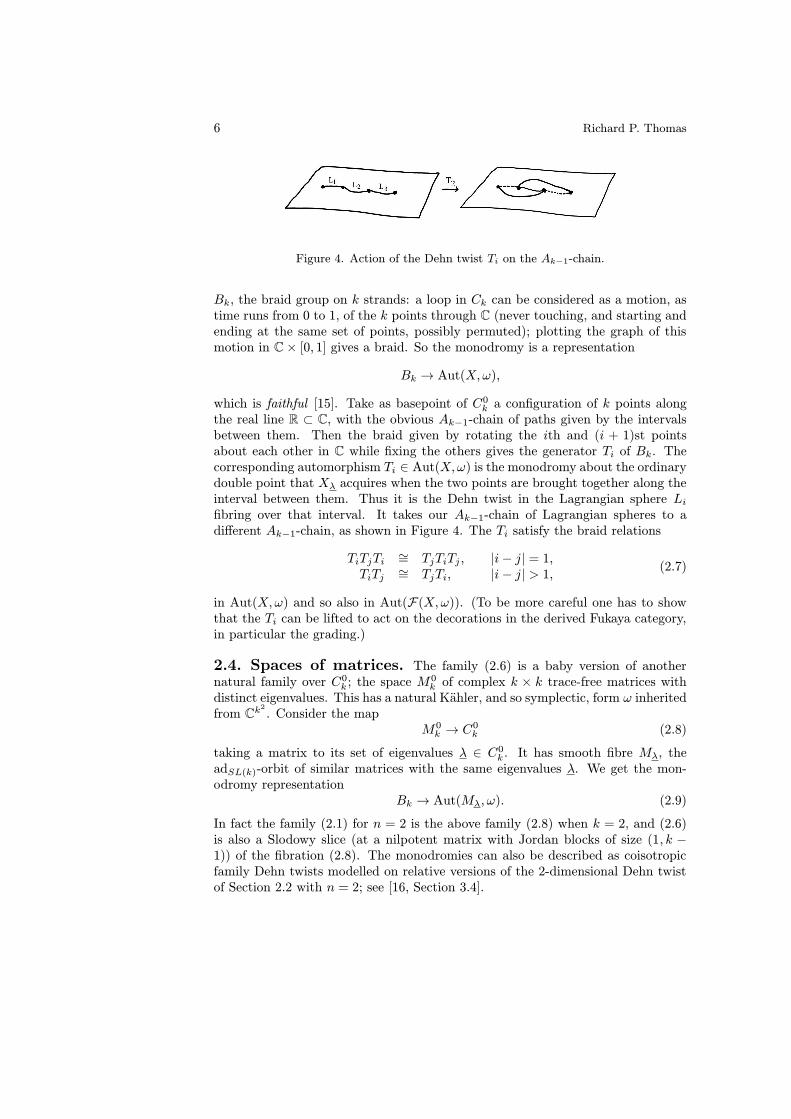
Figure 4. Action of the Dehn twist Ti on the Ak−1-chain.
Bk, the braid group on k strands: a loop in Ck can be considered as a motion, astime runs from 0 to 1, of the k points through C (never touching, and starting andending at the same set of points, possibly permuted); plotting the graph of thismotion in C× [0, 1] gives a braid. So the monodromy is a representation
Bk → Aut(X,ω),
which is faithful [15]. Take as basepoint of C0k a configuration of k points alongthe real line R ⊂ C, with the obvious Ak−1-chain of paths given by the intervalsbetween them. Then the braid given by rotating the ith and (i + 1)st pointsabout each other in C while fixing the others gives the generator Ti of Bk. Thecorresponding automorphism Ti ∈ Aut(X,ω) is the monodromy about the ordinarydouble point that Xλ acquires when the two points are brought together along theinterval between them. Thus it is the Dehn twist in the Lagrangian sphere Lifibring over that interval. It takes our Ak−1-chain of Lagrangian spheres to adifferent Ak−1-chain, as shown in Figure 4. The Ti satisfy the braid relations
TiTjTi ∼= TjTiTj , |i− j| = 1,TiTj ∼= TjTi, |i− j| > 1,
(2.7)
in Aut(X,ω) and so also in Aut(F(X,ω)). (To be more careful one has to showthat the Ti can be lifted to act on the decorations in the derived Fukaya category,in particular the grading.)
2.4. Spaces of matrices. The family (2.6) is a baby version of anothernatural family over C0k ; the space M
0k of complex k × k trace-free matrices with
distinct eigenvalues. This has a natural Kahler, and so symplectic, form ω inheritedfrom Ck
2
. Consider the mapM0k → C
0k (2.8)
taking a matrix to its set of eigenvalues λ ∈ C0k . It has smooth fibre Mλ, theadSL(k)-orbit of similar matrices with the same eigenvalues λ. We get the mon-odromy representation
Bk → Aut(Mλ, ω). (2.9)
In fact the family (2.1) for n = 2 is the above family (2.8) when k = 2, and (2.6)is also a Slodowy slice (at a nilpotent matrix with Jordan blocks of size (1, k −1)) of the fibration (2.8). The monodromies can also be described as coisotropicfamily Dehn twists modelled on relative versions of the 2-dimensional Dehn twistof Section 2.2 with n = 2; see [16, Section 3.4].

An exercise in mirror symmetry 7
A different slice of the family (2.8) when k = 2m is considered by Seidel andSmith [27]. Let SS2m denote the space of trace-free matrices A with distincteigenvalues and the following block form
A :=
A1 I2 0 0 0A2 0 I2 0 0. . . . . .Am−1 0 0 0 I2Am 0 0 0 0
, (2.10)
where Ai is any 2× 2 matrix, A1 is trace-free, and I2 is the 2× 2 identity matrix.Again the eigenvalue map makes this a smooth symplectic bundle
SS2m → C02m, (2.11)
with monodromy representation B2m → Aut(SSλ, ω) on a fibre SSλ.
2.5. The Manolescu isomorphism. Manolescu [18] found another beau-tiful relationship between the Seidel-Smith family and the basic family (2.6) overC02m. Namely, he showed that SS2m can be identified with an explicit open subsetof the relative Hilbert scheme of m points on the smooth fibres of the family ofALE surfaces given by (2.6) with n = 2 and deg p = 2m.Manolescu described his isomorphism by ingenious algebraic manipulation, but
it is possible to describe it geometrically as follows. We fix m and work on onefibre SSλ, fixing the degree 2m monic polynomial pλ(x) with roots λ that is thecharacteristic polynomial of matrices in SSλ.Since the Ai commute with the other 2× 2 blocks in A (2.10), we can evaluate
the determinant of xI2m −A blockwise to give the 2× 2 matrix polynomial
A(x) := I2xm −A1x
m−1 −A2xm−2 − . . .−Am (2.12)
with determinant det(A(x)) = pλ(x).In fact it is convenient to work with the matrices
B(x) := A(x)J = Jxm − (A1J)xm−1 − (A2J)x
m−2 − . . .− (AmJ), (2.13)
where multiplication by
J =
(0 1−1 0
)
, J2 = −1,
is invertible, preserves determinants, and takes trace-free matrices to symmetricmatrices. Therefore writing the polynomial-valued 2×2 matrices B(x) in the form
B(x) =
(V (x) U(x)W (x) X(x)
)
, (2.14)
we have that U and −W are monic of degree m, U and W have equal coefficientsof xm−1 (the trA1 = 0 condition), and V, X have degree m− 1 and satisfy
det(B(x)) = V (x)X(x)− U(x)W (x) = pλ(x). (2.15)

8 Richard P. Thomas
Matrices B(x) (2.14) satisfying these conditions are entirely equivalent to matricesA ∈ SSλ (2.10).Considering B(x) to be an endomorphism of the trivial rank 2 bundle over Cx,
we study it via its spectral curve. Plotting the two eigenvalues y1(x), y2(x) of B(x)gives a curve
CB := {(x, y) : det(yI2 −B(x)) = 0} ⊂ Cx × Cy
double covering Cx. Expanding out gives the equation of CB ⊂ Cx × Cy as
y2 − tr(B(x))y + pλ(x) = 0. (2.16)
Over this curve is the natural line subbundle Eig → CB of the trivial rank twobundle given by the corresponding eigenspace of B(x). At (x, y) ∈ CB , yI2−B(x)has rank≤ 1 and top row (y−V (x) −U(x)), so an obvious element of the kernelis its perpendicular (
U(x)
y − V (x)
)
.
This defines a generator of the eigenspace except when it vanishes, i.e. except atthe points (αi, V (αi)), where αi are the m roots of U(x). (And from (2.14) or(2.16) one sees that indeed y = V (x) is on one branch of CB at the roots of U(x);the other branch being y = X(x).)So we have exhibited a section of Eig vanishing on the length-m divisor D =
{(αi, V (αi))}, or, more precisely,
D = {U(x) = 0 = y − V (x)} ∈ Hilbm CB . (2.17)
In particular, at smooth points of CB , we find that
Eig ∼= OCB (D). (2.18)
Write the equation (2.16) of the curve CB ⊂ Cx × Cy as
y(tr(B(x)− y) = pλ(x).
Plotting the graph of the other eigenvalue
Y = tr(B(x))− y
of B(x) embeds CB in
Sλ := {yY = pλ(x)} ⊆ Cx × Cy × CY . (2.19)
This is the affine blow up of C2xy in the points (λi, 0) defined by y = 0 = pλ(x),and is isomorphic to the ALE surface (2.6) (with n = 2 and k = 2m). (The usualblow up is given by the same equation in C2 × P1Y but we are removing the locusY = ∞ – the proper transform of y = 0 – to get Sλ. Since by (2.15) the curve

An exercise in mirror symmetry 9
CB ⊂ C2 never hits y = 0 except at the roots of pλ(x) it more naturally lies in theblow up (2.19) of C2 than in C2 itself. This will help us to invert the constructionbelow. What is going on here is that a point (x, y) ∈ CB determines the othereigenvalue Y = pλ(x)/y by (2.15) except when y = 0. At such points, i.e. when xis one of the roots λi, the fact that y = 0 tells us nothing as we already knew thatCB goes through (λi, 0) by (2.15). To invert the construction we will need to knowthe gradient of CB at this point instead, and this determines the other eigenvalue.The blow up (2.19) achieves this.)Manolescu’s map then maps A (2.10) (or equivalently B(x) (2.13)) to the image
of the divisor D (2.17) under the inclusion
Hilbm CB ⊂ Hilbm Sλ.
By its definition (2.17) we see that D projects to the length m subscheme {U(x) =0} ∈ Hilbm Cx under the obvious projection Sλ → Cx. In other words no part ofD is tangent to the fibres of this projection and the restriction of the projectionto D is an isomorphism. This proves one half of the following.
Theorem 2.20. [18, Prop 2.7] The above construction gives an isomorphism be-tween the space SSλ and the open subset of Hilb
m Sλ consisting of subschemeswhose projection to Cx also have length m.
The proof of the converse is now easy. Fix D ∈ Hilbm Sλ whose projection toCx has length m. This defines a unique degree m monic polynomial U(x) withthose roots. The function y|D defines a function on the projection of D in Cx, andthere is a unique degree m− 1 polynomial V (x) on Cx whose restriction takes thesame values. Similarly Y |D defines X(x). Finally a degree m polynomial W (x),with leading two coefficients −1 and the xm−1 coefficient of U(x) respectively, isuniquely determined by comparing coefficients in the equation (2.15), using thefact that the coefficient of x2m−1 in pλ is
∑λi = trA = 0. This determines B(x)
(2.14), as required.More geometrically, we are saying that D determines the curve CB through
it, and (at least at smooth points of CB) the eigensheaf Eig = OCB (D) (2.18).Pushing this down gives the trivial rank two bundle, on Cx, while the scalar en-domorphism y descends to an endomorphism B(x) of this trivial rank two bundle.This is the classical spectral curve construction for Higgs bundles [10]. I only re-cently discovered that the link to Hilbert schemes was discovered 15 years ago byHurtubise [11].
2.6. Digression – fixed point locus. In [28] Seidel and Smith also con-sider the involution on SSλ given by replacing each Ai by its transpose. Thefixed point locus consists of those matrices A(x) (2.12) which are symmetric; aftermultiplying by J we get those matrices B(x) (2.13) which are trace-free.This fixes the eigenvalues of B(x) (since its determinant is also fixed (2.15))
and so the (smooth) spectral curve,
CB := {y2 = pλ}. (2.21)
10 Richard P. Thomas
Restricted to this locus, the above gives a geometric description of the algebraicconstruction in [28] (a precursor [29] of Manolescu’s construction). The result isan embedding of the fixed point locus of SSλ in
Symm CB .
The image is the complement of the “hyperelliptic locus” of Symm CB – i.e. itis the length-m subschemes of the hyperelliptic curve CB → Cx whose projectionto Cx also have length m. In [28] Seidel and Smith use this to make a beauti-ful link between their construction of Khovanov cohomology (of Section 2.8) toOzsvath-Szabo theory. So in this setting the passage from Ozsvath-Szabo theoryto Khovanov cohomology is a form of complexification, replacing the Riemannsurface (2.6 with n = 1) by the hyperkahler ALE surface (2.6 with n = 2) – i.e.replacing (2.21) by (2.19) – and taking Hilbm of either.
2.7. ALE spaces as affine blow ups. Buried in the description of theManolescu embedding we saw how to describe the ALE surfaces Sλ (2.6) as affineblow ups. Here we emphasise the construction and a consequence.Fixing monic p with roots λ, we consider the ALE surface
Sλ = {xy = p(t)} ⊂ Cx × Cy × Ct (2.22)
with its obvious projection to Cx × Ct. This is an isomorphism except over thepoints x = 0 = p(t) of C2, where the fibre is an exceptional copy of C. This isthe affine blow up of C2 in x = 0 = p(t): the usual blow up given by the sameformula in Cx×P1y×Ct but with y =∞ (the proper transform of the t-axis x = 0)removed.The usual Ak−1-chain of Lagrangian S
2s in (2.22) can be seen as follows. Pickan Ak−1-chain of paths in Ct between the roots of p(t). Multiplying by the radiusε circle about the origin in Cx gives k Lagrangian S1× [0, 1] tubes in C2. Blow upC2 symplectically by removing balls of radius ε about each point of x = 0 = p(t)and collapsing the Hopf fibration on the boundary S3s. This collapses the tubesto Lagrangian S2s forming our Ak−1-chain; see for instance [31].As Ivan Smith explained to me, this can also be seen as a “spinning” ([26] is a
good recent reference) of Ct over the roots λ of p(t). The fibres of the projectionto Ct are conics C∗ (the fibres of Cx × Ct → Ct with the t-axis (x = 0) removed)except over the roots of p(t) where we get the singular conics C∪0C (the exceptionalfibre union the original fibre Cx).What is nice about the description as an affine blow up is that it demonstrates
natural maps between the ALE spaces that are compatible with the Ak-chains.Ignoring the centre of mass condition for simplicity, let
Sk−1 ⊂ Sk−1
denote the ALE surface (2.22) with λ = (1, 2, . . . , k) inside the full blow up of C2
in the points (0, 1), (0, 2), . . . , (0, k).Then Sk is the blow up of Sk−1 in the point (0,∞, k+1). On removing y =∞
we get a projection Sk → Sk−1. And since we have removed the blow up point

An exercise in mirror symmetry 11
(0,∞, k + 1), we also get an inclusion Sk−1 ↪→ Sk which is a right inverse. Thesemaps are holomorphic; there are also maps preserving the real symplectic structureonce we remove a ball about (0,∞, k + 1) from Sk−1, which will be sufficient forour needs in the next Section.
2.8. The Seidel-Smith construction. Seidel and Smith managed toproduce an invariant of links using the space SS2m (2.10). Via the Manolescuisomorphism, and using plait closure in place of braid closure, the constructionshould become the following. (Since the technical details have only been carriedout carefully [27] in the open subset SSλ ⊂ Hilb
m Sλ, the following is partly con-jectural, and should be thought of only as motivation for the mirror construction.In particular Hilbm Sλ is not an exact symplectic manifold, so the definition ofFloer cohomology needs some care.)We fix one of the ALE surfaces (2.22), writing it as
S2m−1 :=
{
xy =
2m∏
i=1
(t− λi)
}
⊂ Cx,y × Ct,
where λ is a collection of 2m distinct numbers λi ∈ C (with average zero). We alsochoose an A2m−1-configuration of paths γi running between them, as in Figure 4,and so an A2m−1-chain of Lagrangian spheres Li ⊂ S2m−1.In turn this defines the Lagrangian (S2)m
L = Lm := L1 × L3 × . . .× L2m−3 × L2m−1 (2.23)
in the Hilbert schemeHm := Hilb
m S2m−1,
via the map L1 × . . . × L2m−1 ⊂ (S2m−1)m → Symm S2m−1−→ Hilb
m S2m−1.(Since the L2i−1 are disjoint, the map’s image lies in the complement of the largediagonal, over which Hilbm S2m−1 → Sym
m S2m−1 is an isomorphism.)The relative Hilbert schemes of the family of Sλs (2.6) gives a quasi-projective
family over C02m. Taking monodromy, we see that the braid group lifts to thesymplectomorphism group of Hilbm S2m−1. The Kahler form is the one pulledback via the resolution Hilbm → Symm, minus ε[E], where E is the exceptionaldivisor. By making ε→ 0 we can ensure that the action of β ∈ B2m is arbitrarilyclose, away from the exceptional locus, to the action of β× . . .×β on Symm S2m−1.Then for any β ∈ Bm define the braid invariant
SS∗(β) := HF ∗+m+w(L, βL) (2.24)
to be the Floer cohomology of L and its image under β (assuming the technicaldetails can be overcome to define this, and as a graded C-vector space rather thana module over a Novikov ring). Here the writhe w is the number of positive minusthe number of negative crossings in the braid β.In fact SS∗(β) should be an invariant of the isotopy class of the link given by
the plait closure of β. By a result of Birman [3], modified slightly in [2], and the
12 Richard P. Thomas
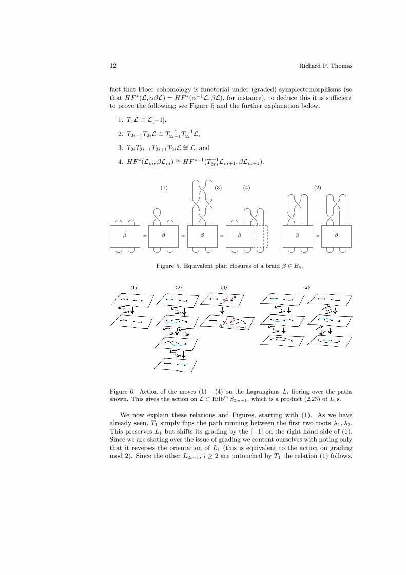
fact that Floer cohomology is functorial under (graded) symplectomorphisms (sothat HF ∗(L, αβL) = HF ∗(α−1L, βL), for instance), to deduce this it is sufficientto prove the following; see Figure 5 and the further explanation below.
1. T1L ∼= L[−1],
2. T2i−1T2iL ∼= T−12i−1T
−12i L,
3. T2iT2i−1T2i+1T2iL ∼= L, and
4. HF ∗(Lm, βLm) ∼= HF ∗+1(T±12mLm+1, βLm+1).
β ' ' ' ββ 'β β
(2)(3)(1)
β
(4)
Figure 5. Equivalent plait closures of a braid β ∈ B4.
Figure 6. Action of the moves (1) – (4) on the Lagrangians Li fibring over the pathsshown. This gives the action on L ⊂ Hilbm S2m−1, which is a product (2.23) of Li s.
We now explain these relations and Figures, starting with (1). As we havealready seen, T1 simply flips the path running between the first two roots λ1, λ2.This preserves L1 but shifts its grading by the [−1] on the right hand side of (1).Since we are skating over the issue of grading we content ourselves with noting onlythat it reverses the orientation of L1 (this is equivalent to the action on gradingmod 2). Since the other L2i−1, i ≥ 2 are untouched by T1 the relation (1) follows.

An exercise in mirror symmetry 13
Secondly we consider (3). As shown in Figure 6, T2iT2i−1T2i+1T2i simply swapsL2i±1 (and leaves the other L2j−1 alone). But in Hilb
m S2m−1 the order of thefactors of L is unimportant, so (3) follows.Relation (4) (stabilisation as we increase the number of strands in our braid,
or Markov II as it is called in [27]) is slightly more involved. The left hand sideis computed in Hm, with β an element of B2m. The right hand side takes placein Hm+1, with β considered as an element of B2m+2 via the standard inclusionB2m ↪→ B2m+2. Here we are using the inclusion of ALE spaces S2m−1 ⊂ S2m+1 ofSection 2.7.In Figure 6 is drawn part of an arbitrary O(2)-invariant Lagrangian A which
is generated in F(S2m−1) by Li, i ≤ 2m− 1 (βLm in (4) being a product of suchthings). We have drawn intersections of A with L2m−1 in either the root λ2m orelsewhere. This corresponds to a splitting
HF ∗(L2m−1, A) ∼= HF∗+1(L2m, A) ⊕ HF
∗(T2mL2m−1, A) (2.25)
coming from the exact triangle (cf. (2.4))
L2m−1 → T2mL2m−1 → L2m (2.26)
in F(S2m−1). (One can show that HF ∗( ∙ , A) applied to the second arrow vanishesfor A = Li, i ≤ 2m − 1, and so for any A, to give the splitting (2.25).) The firstsummand in (2.25) corresponds to the intersections at the root λ2m; these comefrom intersections with the next Lagrangian L2m along via cup product with theHF 1(L2m, L2m−1) class of the intersection of L2m−1 and L2m (the extension classof the triangle (2.26)). The other intersection points are those which survive whenL2m−1 is Dehn twisted about L2m, as shown in Figure 6, and form the secondsummand of (2.25).Since A has no intersections with L2m+1 the first summand is isomorphic to
HF ∗+1(T2mL2m+1, A), as can also be seen from Figure 6. The upshot is thatif A is a product of Lagrangians of the form A, the intersection points used tocalculate HF ∗(Lm,A) can be matched with intersection points used to calculateHF ∗+1(T2mLm+1,A). More precisely their Floer cohomologies can be matchedusing (2.25). Applied to A = βLm this gives (4).Finally we come to relation (2). We calculate on S2n−1 that both T2i−1T2i
and T−12i−1T−12i leave L2j+1 alone for j 6= i, i − 1, and take L2i−1 to L2i. This is
clear from Figure 6. Their actions on L2i+1 differ, however. They both take it toconnect sums of L2i−1, L2i and L2i+1, but in the opposite direction:
T2i−1T2iL2i+1 ∼= L2i+1#L2i#L2i−1, (2.27)
T−12i−1T−12i L2i+1
∼= L2i−1#L2i#L2i+1. (2.28)
Here # is the graded Lagrangian connect sum [22, 33], and is not symmetric. Itcan be described in an O(2)-symmetric manner by the connect-summed paths inFigure 6 – with the connect sums in opposite directions corresponding to pathsabove and below their intersection point.

14 Richard P. Thomas
The two Lagrangians (2.27, 2.28) are certainly not Hamiltonian isotopic inS2m−1, so that T2i−1T2iL and T
−12i−1T
−12i L are not Hamiltonian isotopic in either the
product (S2m−1)m or symmetric product Symm S2m−1. However Seidel and Smith
prove they are Hamiltonian isotopic in SS2m, and therefore also in Hilbm S2m−1.
We want to think about this categorically as follows.
In the derived Fukaya category, we see T2i−1T2iL and T−12i−1T
−12i L as extensions
of the same objects in the opposite direction. On deforming the symplectic spaceSymm S2m−1 to Hilb
m S2m−1 (by “inflating” the exceptional divisor – subtracting asmall amount of the class of the exceptional divisor from the degenerate symplecticform pulled back from Symm S2m−1) the Lagrangians T
±12i−1T
±12i L deform because
both L and the symplectomorphisms Ti do. However the pieces L2i±1 × L2i ofthe extensions do not deform as Lagrangians – the class [E] restricts to a nonzeroclass thereon (because L2i±1 intersects L2i inside S2m−1). And then for generalreasons, if two extensions of the same pieces deform while the pieces do not thenthe deformations of the extensions become isomorphic. The algebro-geometricanalogue of this will be clearer to see in Section 5.
Using slightly different techniques in a fibre of SS2m, Seidel and Smith provecarefully that they get an invariant of links up to isotopy. Conjecturally theirinvariant can be derived from the famous Khovanov cohomology KH∗,∗ ⊗ C [14]by a certain collapse of the latter’s bigrading. In the algebro-geometric mirrordescribed later, it will in fact be possible to get the full bigrading and prove theisomorphism to KH∗,∗ ⊗ C.
3. Simultaneous resolution
In each of the examples (2.1), (2.6), (2.8) and (2.11) – in the first two cases only indimension n = 2 – the families have a remarkable property. The complete familyX → B (including the singular fibres now) can be pulled back to a new familyX ′ → B′ via a finite basechange B′ → B, such that X ′ admits a simultaneousresolution
π : X → X ′.
This is a map which is birational, and a resolution of singularities on each fibre.In particular on each smooth fibre it restricts to an isomorphism. So the smoothfibres fit together with the resolutions of the singular fibres in a smooth familyX → B′. Thus the smoothings and resolutions of the singular fibres of X → B arediffeomorphic (something which is obviously not true for the n = 1 dimensionalnode (2.1), for instance) and is related to the fact that they are hyperkahler [12].
3.1. Surface ordinary double point. The simplest case is the smooth-ing of the surface ordinary double point,
X = {x2 + y2 + w2 = t} ⊂ C3xyw × Ct → Ct.

An exercise in mirror symmetry 15
If we pull this back by the double cover t 7→ t2 of the base then the total spacebecomes singular itself, with the threefold ordinary double point singularity
X ′ = {x2 + y2 + w2 = t2} ⊂ C3xyw × Ct → Ct. (3.1)
Setting X = x+ iy, Y = x− iy, T = t+ w,W = t− w this becomes
X ′ = {XY = TW} ⊂ C4
fibring over C by the function (T+W )/2. Blowing up the Weil divisor (X = 0 = T )gives a resolution X → X ′ which is an isomorphism away from the origin. Moreexplicitly, X is the graph of the rational function X/T = W/Y : X ′ → P1 inX ′ × P1:
X := {(X,Y, T,W, [λ : μ]) ∈ C4 × P1 : XY = TW, μX = λT, μW = λY }.
Then X → X ′ is an isomorphism on all of the smooth fibres of (3.1), and replacesthe central fibre’s surface ordinary double point by its minimal resolution – i.e. itsblow up with a P1 exceptional set C. (So the exceptional set of the whole familyis this C ∼= P1, which is not a divisor: X → X ′ is a small resolution).
Figure 7. Simultaneous resolution X of the family (3.1), with the Lagrangian vanishingcycles L ∼= S2 limiting to the holomorphic exceptional curve C ∼= P1.
We picture this in Figure 7. By its definition as a vanishing cycle, under sym-plectic parallel transport the Lagrangian L limits to the holomorphic exceptionalP1 = C. This is remarkable but no contradiction; the pull back of the standardKahler form from X ′ is symplectic on the general fibre (and zero on restriction toL) but degenerate on the central fibre (it is precisely zero along C). One could per-turb to get a nondegenerate Kahler form on X , giving nonzero area to C, but thiswould then also have nonzero area on the (homologous) L which would thereforecease to be Lagrangian.
One can also ask what the limit of the Dehn twists is on the central fibre.Consider the graph in Xε ×Xε of the monodromy about the circle of radius ε. As
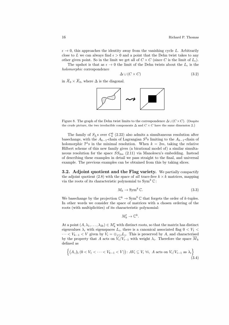
16 Richard P. Thomas
ε → 0, this approaches the identity away from the vanishing cycle L. Arbitrarilyclose to L we can always find ε > 0 and a point that the Dehn twist takes to anyother given point. So in the limit we get all of C × C (since C is the limit of Lε).The upshot is that as ε → 0 the limit of the Dehn twists about the Lε is the
holomorphic correspondence
Δ ∪ (C × C) (3.2)
in X 0 ×X 0, where Δ is the diagonal.
Figure 8. The graph of the Dehn twist limits to the correspondence Δ∪ (C×C). (Despitethe crude picture, the two irreducible components Δ and C × C have the same dimension 2.)
The family of Sλ s over C0k (2.22) also admits a simultaneous resolution after
basechange, with the Ak−1-chain of Lagrangian S2s limiting to the Ak−1-chain of
holomorphic P1s in the minimal resolution. When k = 2m, taking the relativeHilbert scheme of this new family gives (a birational model of) a similar simulta-neous resolution for the space SS2m (2.11) via Manolescu’s embedding. Insteadof describing these examples in detail we pass straight to the final, and universalexample. The previous examples can be obtained from this by taking slices.
3.2. Adjoint quotient and the Flag variety. We partially compactifythe adjoint quotient (2.8) with the space of all trace-free k× k matrices, mappingvia the roots of its characteristic polynomial to Symk C :
Mk → Symk C. (3.3)
We basechange by the projection Ck → Symk C that forgets the order of k-tuples.In other words we consider the space of matrices with a chosen ordering of theroots (with multiplicities) of its characteristic polynomial:
M ′k → Ck.
At a point (A, λ1, . . . , λ2k) ∈M ′k with distinct roots, so that the matrix has distincteigenvalues λi with eigenspaces Li, there is a canonical associated flag 0 < V1 <∙ ∙ ∙ < Vk−1 < V given by Vi = ⊕j≤iLj . This is preserved by A, and characterisedby the property that A acts on Vi/Vi−1 with weight λi. Therefore the space Mkdefined as{(A, λ, (0 < V1 < ∙ ∙ ∙ < Vk−1 < V )
): AVi ⊆ Vi ∀i, A acts on Vi/Vi−1 as λi
}
(3.4)

An exercise in mirror symmetry 17
has a forgetful map toM ′k which is an isomorphism over the good locus of matriceswith distinct eigenvalues. In fact Mk →M ′k is a simultaneous resolution, restrict-ing over each fibre of M ′k → Ck to a resolution of singularities. The central fibreis the cotangent bundle T ∗Fl of the Flag variety, because its fibre over a point(0 < V1 < ∙ ∙ ∙ < Vk−1 < V ) ∈ Fl is
{A : V → V : AVi ⊆ Vi−1}.
It provides a resolution of the central fibre of Mk → Symk C, i.e. of the nilpotent
cone of matrices with no nonzero eigenvalues. The general fibre is diffeomorphicto it; in fact it is symplectomorphic to T ∗Fl with its canonical real symplecticstructure as the cotangent bundle of a real manifold.
A similar picture to Figure 7 holds. While Fl is a holomorphic subvariety ofthe central fibre, it is the limit of Lagrangian vanishing cycles Fl ⊂ T ∗Fl in thegeneral fibre.
In the central fibre T ∗Fl live the divisors
Ni := π∗i T∗Fli ⊂ T
∗Fl, (3.5)
where πi : Fl → Fli is the map to the partial flag variety that forgets the ithterm Vi in the flag. In the general fibre (seen as symplectomorphic to T
∗Fl) theyare coisotropic with characteristic foliation πi|Ni a fibration by isotropic S
2s. Asλi and λi+1 come together in the base Sym
k C = {eigenvalues} (3.3), Ni is therelative vanishing cycle that collapses along this characteristic foliation to a familyof surface ordinary double points. Doing the family generalised Dehn twist aboutNi ([21, Section 1.4], [19, Section 2.3]) should give the braid group of symplecticmonodromies of (2.9). The limit of the graphs of these symplectomorphisms is thesubvariety
Δ ∪ (Ni ×Fli Ni) ⊂ T∗Fl × T ∗Fl. (3.6)
4. Homological mirror symmetry
Kontsevich’s homological mirror symmetry conjecture [17] is an amazing categor-ical expression of Witten’s formulation of mirror symmetry in terms of A- andB-models. It has become a vast subject that we will only touch on through ourexample.
Roughly speaking, Kontsevich says that two closed Calabi-Yau manifolds shouldbe considered as mirror pairs when the derived Fukaya category of one is isomor-phic to the derived category of coherent sheaves on the other. Symplectic geometry(the “A-model”) on one side is equated with complex geometry (the “B-model”) onthe other side. In particular the plentiful automorphisms of a symplectic manifoldshould be mirrored not by holomorphic automorphisms of the mirror (of whichthere are few) but by autoequivalences of its derived category.

18 Richard P. Thomas
4.1. Surfaces. For the examples of the last section, passing from the generalfibre to the resolution of the central fibre (using symplectic parallel transportand simultaneous resolution) gives a cheap way to swap complex and symplecticstructures. As we have seen, Lagrangian submanifolds can become, in the limit,holomorphic (in fact complex Lagrangian, in the canonical holomorphic symplecticstructure). Taking the structure sheaves of these limits means we have turnedobjects of the derived Fukaya category into objects of the derived category ofcoherent sheaves.So it seems a reasonable guess that the mirror of the (symplectic) general fi-
bre might be related to the (holomorphic) resolution of the central fibre. (Thatmirror symmetry is so simple here, not even changing the topology, is a feature ofhyperkahler manifolds, with the mirror map being related to hyperkahler rotation.To make this more precise would involve complexifying our symplectic forms withB-fields, putting connections with curvature B|L on our Lagrangians L, introduc-ing coisotropic branes, worrying about noncompactness, and working much harder.But we use mirror symmetry here only as a motivational guide.)So in the simplest case we would like to think of the mirror of the symplectic
manifold T ∗S2 (the smoothing of the surface ordinary double point) as somethinglike the complex surface S = T ∗P1 (the resolution of the surface ordinary doublepoint). As usual we denote the Lagrangian S2 by L and the holomorphic P1 byC, so we would like mirror symmetry to relate
L ∈ F(T ∗S2) to OC(−1) ∈ D(S),
where D denotes the bounded derived category of coherent sheaves with compactsupport. (Work of Auroux and Seidel suggests one should remove certain locifrom T ∗S2 and T ∗P1 before they can sensibly be considered as mirror, but forour heuristic purposes we can ignore this.) The twist by the line bundle O(−1) isunimportant (since it defines an autoequivalence of D(S)) and is just for conve-nience.Since the graph of the Dehn twist TL about L limits (3.2) to the holomorphic
subvariety
Δ ∪ (C × C)ι↪→ S × S, (4.1)
it is natural to use this as a holomorphic correspondence on S. In fact we wouldlike to lift this to an action on D(S), mirror to the induced action of TL onF(T ∗S2). So we might use the structure sheaf of (4.1) as a Fourier-Mukai kernel.For convenience we twist by the line bundle L which is OS(C) on Δ glued toO(−1,−1) on C × C (both are isomorphic to OC(−2) on ΔC):
TC := π2∗(ι∗L ⊗ π
∗1( ∙ )
): D(S)→ D(S).
(Here π1, π2 : S × S → S are the obvious projections, and the functors ⊗ and π2∗are derived. It turns out that using the untwisted structure sheaf gives the inverseof the functor TC ; I don’t know if this is significant or a coincidence.) Equivalently,the action of TC on E ∈ D(S) is
E 7→ TCE = Cone(RHom(OC(−1), E)⊗OC(−1)→ E
), (4.2)

An exercise in mirror symmetry 19
where the arrow is the obvious evaluation map. (Taking E to be a complex ofinjectives, this map is canonical rather than defined up to homotopy, so the coneturns out to be functorial here [30].) Compare its mirror (2.3, 2.4).More generally, the simultaneous resolution of the family of ALE surfaces (2.22)
has central fibre the minimal resolution of
{xy = tk} ⊆ C3. (4.3)
Call this S, with its Ak−1-chain of exceptional −2-curves Ci ⊂ S (the limit ofan Ak−1-chain of Lagrangian vanishing cycles Li on a general fibre). In fact thesheaves Ai := OCi(−1) satisfy the following homological definition of an Ak−1-chain in any derived category of coherent sheaves.
Definition 4.4. [30] Objects Ai ∈ D(S), i = 1, . . . , k − 1 form an Ak−1-chain ofn-spherical objects if for all i, j,
• Ext∗(Ai, Ai) ∼= H∗(Sn,C),
• Ai ⊗ ωS ∼= Ai,
•⊕p Ext
p(Ai, Aj) =
{C |i− j| = 1,0 |i− j| > 1.
For us n = 2, and the second, Calabi-Yau condition always holds since thecanonical bundle ωS of S is trivial. One can then define the Dehn twists about theAi as in (4.2) by
TAiE := Cone(RHom(Ai, E)⊗Ai → E), (4.5)
or by Fourier-Mukai transform with the kernel
Cone(A∨i �Ai → OΔ
).
Here ∨ denotes derived dual, and the arrow is restriction to the diagonal followedby evaluation (trace).
Theorem 4.6. [15, 30] If the Ai form an Ak−1-chain then the Ti = TAi define a(weak) faithful action of the braid group Bk ↪→ Aut(D(S)).In particular, the Ti are invertible and satisfy the braid relations
TiTjTi ∼= TjTiTj , |i− j| = 1,TiTj ∼= TjTi, |i− j| > 1.
So our putative mirrors of Dehn twists really satisfy the same relations as theoriginal twists (2.7). And we have put things in a more categorical framework,allowing twists around arbitrary spherical objects, as mirror symmetry suggestsshould be possible – according to Kontsevich’s conjecture, all mirror symmetryneeds to see is categorical properties, rather than specific geometry. For more onmirror symmetry for ALE surfaces see [13].

20 Richard P. Thomas
4.2. Higher dimensions. Our other examples of families over C0k fit into asimilar hyperkahler mirror symmetry picture. In fact they all follow from the caseof the space of matrices of Section 3.2 by taking slices. In much the same way asdescribed above, the family Dehn twists around the divisors Ni limit to the Fourier-Mukai transforms with kernels the structure sheaves of the limits Δ∪ (Ni×Fli Ni)(3.6) of the graphs of these symplectomorphisms. Up to twisting by a line bundle,these are the relative versions of the derived category Dehn twist (4.5), with action
E 7→ Cone(ιi∗p
∗i pi∗ι
!iE → E
).
Here the arrow is evaluation, and pi and ιi are the obvious maps
Niιi↪→ T ∗Fl
↓pi
T ∗Fli.
(4.7)
Again these define autoequivalences Ti : D(T∗Fl) → D(T ∗Fl) which satisfy the
braid relations [1, 16]. In fact the Ti (both here and on the slices S of the last sec-tion) even admit natural transformations between them which satisfy the relationsof the braid cobordism category, and these give rise to maps between the Khovanovcohomology groups of links of the next Section, when we fix a link cobordism. Butwe refer to [16] for this further extension of mirror symmetry.The braid relations in this case aremuch harder than those in 2 dimensions. But
Manolescu’s isomorphism means that they follow from the simple two dimensionalcase for the spaces relevant to Khovanov cohomology.
5. Hilbert schemes of ALE spaces and Khovanovcohomology
By now it should be clear how one would go about trying to mirror the Seidel-Smithconstruction to define Khovanov cohomology in a derived category of coherentsheaves. There is a slice of (3.4) that provides a simultaneous resolution of (thebasechange of) SS2m. The derived category of its central fibre carries a braid groupaction and a complex Lagrangian submanifold that L (2.23) limits to. Taking itsstructure sheaf (and possibly twisting by a line bundle) as an object of the derivedcategory, one would like to show that the Exts from this object to its image undera braid give an invariant of the link closure of the braid.Such a programme has been carried out in beautiful work of Cautis and Kam-
nitzer [5]. In fact they use a compactification of the above space related, via thegeometric Satake correspondence, to the sl(2) representations of the Reshetikhin-Turaev tangle calculus. This has the huge advantage of being generalisable toother Lie algebras [6]. However, as mentioned above, it is also hard work, involv-ing calculations in high dimensions.Manolescu’s isomorphism suggests we might work with something like the
Hilbert scheme of points on S = S2m−1, the minimal resolution of the A2m−1-

An exercise in mirror symmetry 21
singularity (4.3). This reduces most of the work to much simpler calculations withsheaves on the surfaces S2m−1. In fact, by [4, 9] the category
Dm := D(Hilbm S2m−1)
has a canonical identification with the Σm-equivariant derived category of (S2m−1)m,
where the symmetric group Σm permutes the factors:
D(Hilbm S2m−1) ∼= D(Sm2m−1)
Σm . (5.1)
5.1. However. One would expect the right hand side of (5.1) to be mirrorto the Σm-equivariant Fukaya category of Sλ (2.19), which is not the Fukayacategory of its Hilbert scheme, but can be thought of as playing the role of theFukaya category of the singular symplectic space Symm S2m−1. Considering theHilbert scheme as a symplectic deformation of this (subtracting a small multipleof the exceptional divisor of Hilb→ Sym from the degenerate symplectic form onegets by pulling back from Sym) suggests the mirror might be a deformation ofHilbm S2m−1. We will indeed use such a deformation related to the exceptionaldivisor.This is an example where our naive description of mirror symmetry fails. The
mirror of the smoothing Hilbm Sλ of a hyperkahler singularity Hilbm S0 appears
not to be the obvious choice Hilbm S2m−1 (which is birational to a resolution ofHilbm S0) but a deformation thereof.
5.2. The construction. Any E ∈ D(Sm2m−1) defines an element
Σm.E :=⊕
σ∈Σm
σ∗E ∈ D(Sm2m−1)Σm , (5.2)
with its obvious Σm-linearisation. Thus from the spherical objects Li := OCi(−1) ∈D(S2m−1) we define
L = Lm := Σm.(L1 � L3 � . . .� L2m−1) ∈ D(Sm2m−1)
Σm . (5.3)
Equivalently, the object L ∈ D(Hilbm S2m−1) can be described via the Haiman-BKR equivalence (5.1) as follows. As in (2.23), the composition
C1 × C3 × . . .× C2m−1 ↪→ Sm2m−1 → Sym
m S2m−1 Hilbm S2m−1
is an embedding since the C2i−1 do not intersect each other so their product avoidsthe diagonal locus over which the last map is not regular. Then
L = OC1×C3×...×C2m−1(−1,−1, . . . ,−1) ∈ D(Hilbm S2m−1). (5.4)
Any autoequivalence T ∈ Aut(D(S2m−1) induces a canonical autoequivalenceΦ(T ) ∈ Aut(D(Sm2m−1)
Σm) [20]. Its action on objects of the form (5.3) is theobvious one:
Φ(T )(Σm.(E1 � . . .� Em)
)= Σm.
(T (E1)� . . .� T (Em)
). (5.5)

22 Richard P. Thomas
We apply this to the spherical twists Ti := TOCi (−1):
Ti := Φ(Ti)[1] ∈ Aut(D(Sm2m−1)
Σm). (5.6)
Since Φ is a homomorphism, these define generators of a braid group action B2m →Aut(Dm). (The braid relations are homogeneous, so the extra shift [1] makes nodifference.) Thus any β ∈ B2m gives an autoequivalence Tβ ∈ Aut(Dm). We definethe braid invariant
kh∗(β) := Ext∗Dm(L,Tβ L[m]). (5.7)
The shifts in the definitions (5.6, 5.7) match with the shift w +m in the mirrorSeidel-Smith construction (2.24).
5.3. Maps between ALE spaces. To study the dependence of (5.7) onmwe will need the holomorphic analogue (or hyperkahler rotation) of the symplecticmaps between ALE spaces of Section 2.7. So let Sk−1 be the minimal resolutionof Ak−1 := {xk = yz} ⊂ C3. We will exhibit a natural inclusion Sk−1 ⊂ Sk takingthe Ak−1-chain of −2-curves Ci ∼= P1, i = 1, . . . , k − 1 in the former to the firstk − 1 curves of the Ak-chain C1, . . . , Ck−1, Ck in the latter.Consider the blow up of C2 in the ideal (xk, y). Call this Ak−1. It can be
constructed inductively via blow ups and a blow down in smooth centres:
1. Blow up the origin in C2, giving an exceptional divisor E1 ∼= P1.
2. Blow up the point ∞ ∈ E1 (its intersection with the proper transform of thex-axis). We get a new exceptional divisor E2, and the proper transform ofE1 which is a −2-curve C1.
(r) At the rth stage, blow up ∞ ∈ Er−1 to produce a new exceptional divisorEr, and the proper transform of Er−1 is a −2-curve Cr.
After the kth step we get a surface Sk−1 with an Ak−1-chain of −2-curves Ci anda −1-curve Ek; see Figure 9. Now blow down the Ci, i = 1, . . . , k− 1 to get Ak−1.
C1
C2
C3
E4
C1
C2
E3
Figure 9. Newton polygon diagram of the blow up map S2 ← S3. On removing thedivisors corresponding to the dashed lines (the proper transforms of the x-axis) we getan inclusion S2 ⊂ S3 in the opposite direction.
An exercise in mirror symmetry 23
Now Ak−1 = Bl(xk,y) C2 = {μxk = λy} ⊂ C2x,y × P1[λ:μ]. Therefore if we remove
the proper transform {y = 0} = {μ = 0} of the x-axis we can set [λ : μ] = [z : 1]to get the affine variety
{xk = yz} ⊂ C2x,y × Cz,
which is precisely Ak−1. Thus Ak−1 and Sk−1 are partial compactifications ofAk−1 and Sk−1 respectively (since Sk−1 is the minimal resolution of Sk−1).We obtained Sk from Sk−1 by blowing up the latter in the point ∞ ∈ Ek. But
∞ = {y = 0} ∩ Ek lies in the divisor {y = 0} that we remove from Sk−1 to getSk−1, so the inclusion Sk−1 ⊂ Sk−1 lifts to the blow up: Sk−1 ⊂ Sk. Its imageis clearly contained in the open subset Sk, and maps the curves Ci ⊂ Sk−1 to thecorresponding curves Ci ⊂ Sk, as claimed.
As in Section 2.8, to prove that kh∗ is a link invariant under plait closure it issufficient to prove the following; again see Figure 5.
1. T1L ∼= L,
2. T2i−1T2i L ∼= T−12i−1T
−12i L,
3. T2iT2i−1T2i+1T2i L ∼= L, and
4. Ext∗Dm(Lm,Tβ Lm[m])∼= Ext∗Dm+1(T
±12mLm+1,Tβ Lm+1[m+ 1]).
In the last relation we use the inclusion S2m−1 ↪→ S2m+1 exhibited above.
Theorem 5.8. [32] The relations (1), (3) and (4) hold in the categories Dm, but(2) does not.
The proof is reduced by (5.5) to simple computations in D(S2m−1) mirroringthose of Section 2.8.Firstly, T1L2i+1 ∼= L2i+1 for i ≥ 1 by (4.2), because Ext
∗(L1, L2i+1) = 0. SinceExt∗(L1, L1) ∼= H∗(S2,C) we get the exact triangle in D(S2m−1)
L1 ⊕ L1[−2] −→ L1 −→ T1L1.
The first map is the identity on the first factor, so T1L1 ∼= L1[−1]. Therefore by(5.5), T1L ∼= L[−1][1] = L, which proves relation (1).For (2) we note the following calculation on S2m−1. If A,B ∼= P1 are (possibly
reducible) rational curves in S2m−1 intersecting in a single transverse point, thenExt∗(OA,OB) = C[−1] and the resulting exact triangle
OB → TOAOB → OA (5.9)
expresses TOAOB as the nontrivial extension
TOAOB ∼= OA∪B(1, 0). (5.10)
By (1, 0) we mean to twist by the line bundle which is the gluing of the trivialbundle on A and the degree 1 bundle OB(A∩B) on B. (A similar result to (5.10)

24 Richard P. Thomas
holds when OA,OB and TOAOB are all twisted by the same line bundle.) If wedenote this extension by OB#OA it is the mirror of the Lagrangian connect sumof (2.27, 2.28). So, for instance, we picture
TiLi−1 = Li−1#Li = OCi−1∪Ci(0,−1)
as the path in C, running from λi−1 over λi to λi+1, over which its mirror isS1-fibred. Similarly the connect sum in the opposite direction, which is Ti−1Li =OCi−1∪Ci(−1, 0), corresponds to the path under λi. (See [34] for more on thesepictures for objects of D(S2m−1).)Applying this twice we find that
T2i−1T2iL2i+1 = T2i−1OC2i∪C2i+1(−1, 0) = OC2i−1∪C2i∪C2i+1(−1, 0, 0), (5.11)
the second equality following from (5.10) applied to A = C2i−1 andB = C2i∪C2i+1.Similarly,
T−12i−1T−12i L2i+1
∼= OC2i−1∪C2i∪C2i+1(0, 0,−1). (5.12)
Finally T2i−1T2i and T−12i−1T
−12i both take L2i−1 to L2i, by similar calculations
mirroring Figure 6, and they leave L2j+1 alone for j 6= i, i− 1.Since (5.11) and (5.12) are not isomorphic it follows from (5.5) that T2i−1T2i L 6∼=
T−12i−1T−12i L, i.e. (2) does not hold.
Repeated calculations with (5.10) on S2m−1 show that T2iT2i−1T2i+1T2i alsoleaves L2j+1 alone for j 6= i, i− 1, but swaps L2i±1 (see Figure 6):
T2iT2i−1T2i+1T2iL2i±1 = L2i∓1.
Relation (3) then follows again from (5.5).Finally (4) follows just as in the mirror situation of Section 2.8. The exact
triangle (2.26) holds just as well in D(S2m−1) – see (5.9) – giving the splitting
Ext∗(L2m−1, A) ∼= Ext∗+1(L2m, A) ⊕ Ext∗(T2mL2m−1, A)
∼= Ext∗+1(T2mL2m+1, A) ⊕ Ext∗(T2mL2m−1, A)
that replaces (2.25) for any A ∈ D(S2m−1) generated by Li, i ≤ 2m− 1. Relation(4) follows easily; see [32] for full details.
5.4. Deformation. As suggested in Section 5.1, to get something which actsas a better mirror of Hilbm Sλ in which relation (2) holds, we should deform bysomething concentrated on the diagonal.The exceptional divisor E ofHm := Hilb
m(S2m−1)→ Symm(S2m−1) has a class
[E] ∈ H1(ΩHm) despite the noncompactness. (For instance the exact sequence0 → ΩHm → ΩHm(logD) → OD → 0 has extension class in Ext
1(OD,ΩHm); itsimage in Ext1(OHm ,ΩHm) = H
1(ΩHm) is [E].) Via the holomorphic symplecticform ΩHm
∼= THm , and we get a canonical class e ∈ H1(THm), the space of first
order deformations of Hm.Using some twistor theory we get a canonical family H → P1 of holomorphic
symplectic deformations (Ht, σt) of Hm = H0 in the direction of e; see [32]. The

An exercise in mirror symmetry 25
Lagrangian L (5.4) deforms along this deformation because it is disjoint from [E].We show in [32] that the functors Tβ also deform. Both sides of the relations(1), (3) and (4) therefore also deform along H, and by rigidity of the complexesinvolved the equalities continue to hold.Finally then we come to (2). As in (5.11, 5.12) we have (cf. (2.27, 2.28)),
T2i−1T2iL2i+1 ∼= L2i+1#L2i#L2i−1,
T−12i−1T−12i L2i+1
∼= L2i−1#L2i#L2i+1,
are extensions of the same objects but in opposite directions. On deformingHilbm S2m−1 along H, the Lagrangians T
±12i−1T
±12i L deform because both L and
the symplectomorphisms Ti do. However the pieces L2i±1×L2i× . . . of the exten-sions do not deform (essentially because [E] restricts to a nonzero class on theirsupport since L2i±1 intersects L2i inside S2m−1). For general reasons, if two ex-tensions of the same pieces deform while the pieces do not then the deformationsof the extensions become isomorphic.The baby model to keep in mind is to deform S itself so that [C1] and [C2] do
not remain of type (1, 1), but their sum [C1]+ [C2] does. Then neither of OC1(−1)or OC2(−1) deform, but their extensions in different directions,
OC1∪C2(0,−1) and OC1∪C2(−1, 0)
both deform and become isomorphic to OC(−1), where C is the unique (smooth)rational curve that degenerates back to C1 ∪ C2 on the central fibre.
5.5. Bigrading and Khovanov cohomology. There are also C∗-actionson the spaces Si with respect to which the inclusion maps Sk−1 ⊂ Sk are equivari-ant [32]. Since the constructions of this paper are equivariant with respect to thisC∗-action, we get extra C∗-action, and so a bigrading, on the link invariant kh∗.Finally, using the method of [5], one can show that the resulting kh∗,∗ is in
fact Khovanov cohomology KH∗,∗ ⊗C (up to a shift in bigrading). Building up alink from standard cobordisms one presents both kh∗,∗ and KH∗,∗⊗C as iteratedcones on the same standard pieces. (For KH∗,∗ this is Khovanov’s famous “cubeof resolutions”.) Because of some vanishing of Ext groups, this iterated cone isunique.
References
[1] R. Bezrukavnikov, I. Mirkovic, and D. Rumynin, Singular localization and intertwin-ing functors for reductive Lie algebras in prime characteristic. Nagoya Math. Jour.184, 1–55, 2006. math.RT/0602075.
[2] S. Bigelow, A homological definition of the Jones polynomial Geom. & Top. Monogr.4, 29–41, 2002. math.GT/0201221.
[3] J. Birman, On the stable equivalence of plat representations of knots and links,Canad. Jour. Math. 28, 264–290, 1976.

26 Richard P. Thomas
[4] T. Bridgeland, A. King and M. Reid, The McKay correspondence as an equivalenceof derived categories, Jour. A.M.S. 14, 535–554, 2001. math.AG/9908027.
[5] S. Cautis and J. Kamnitzer, Knot homology via derived categories of coherent sheavesI, sl(2)-case, Duke Math. Jour. 142, 511–588, 2008. math.AG/0701194.
[6] S. Cautis and J. Kamnitzer, Knot homology via derived categories of coherent sheavesII, sl(m) case, Invent. Math. 174, 165–232, 2008. arXiv:0710.3216.
[7] K. Fukaya, Mirror symmetry of Abelian variety and multi theta functions, Jour. Alg.Geom. 11, 393–512, 2002.
[8] K. Fukaya, Y.-G. Oh, H. Ohta, and K. Ono, Lagrangian intersection Floer theory:anomaly and obstruction, AMS/IP Stud. in Adv. Math., 46, 2009.
[9] M. Haiman, Hilbert schemes, polygraphs and the Macdonald positivity conjecture,Jour. A.M.S. 14, 941–1006, 2001. math.AG/0010246.
[10] N. Hitchin, The self-duality equations on a Riemann surface, Proc. London Math.Soc. 55, 59–126, 1987.
[11] J. Hurtubise, Integrable systems and algebraic surfaces, Duke Math. Jour. 83, 19-50,1996.
[12] D. Huybrechts, Compact hyper-Kahler manifolds: basic results, Invent. Math. 135,63–113, 1999.
[13] A. Ishii, K. Ueda and H. Uehara, Stability conditions on An-singularities,math.AG/0609551.
[14] M. Khovanov, A categorification of the Jones polynomial. Duke Math. Jour., 101,359-426, 2000. math.QA/9908171.
[15] M. Khovanov and P. Seidel, Quivers, Floer cohomology, and braid group actions, J.Amer. Math. Soc. 15, 203–271, 2002. math.QA/0006056.
[16] M. Khovanov and R. P. Thomas, Braid cobordisms, triangulated categories, and flagvarieties, Homology, Homotopy and Applications 9, 19–94, 2007. math.AG/0609335.
[17] M. Kontsevich, Homological Algebra of Mirror Symmetry, International Congress ofMathematicians, Zurich 1994. Birkhauser, 1995. alg-geom/9411018.
[18] C. Manolescu, Nilpotent slices, Hilbert schemes, and the Jones polynomial, DukeMath. Jour. 132, 311–369, 2006. math.SG/0411015.
[19] T. Perutz, Lagrangian matching invariants for fibred four-maniolds I, Geom. & Top.11, 759–828, 2007. math.SG/0606061.
[20] D. Ploog, Equivariant autoequivalences for finite group actions, Adv. in Math. 216,62–74, 2007. math.AG/0508625.
[21] P. Seidel, unpublished notes, 1997.
[22] P. Seidel, Graded Lagrangian submanifolds, Bull. Soc. Math. France. 128, 103–146,2000. math.SG/9903049.
[23] P. Seidel, A long exact sequence for symplectic Floer cohomology. Topology 42, 1003–1063, 2003. math.SG/0105186.
[24] P. Seidel, Lectures on four-dimensional Dehn twists, In “Symplectic 4-manifolds andalgebraic surfaces”, 231–267, LNM 1938, Springer, 2008. math.SG/0309012.
[25] P. Seidel, Fukaya categories and Picard-Lefschetz theory, Zurich Lectures in Ad-vanced Mathematics, EMS, 2008.
An exercise in mirror symmetry 27
[26] P. Seidel, Suspending Lefschetz fibrations, with an application to local mirror sym-metry, to appear in Comm. Math. Phys., 2010. arXiv:0907.2063.
[27] P. Seidel and I. Smith, A link invariant from the symplectic geometry of nilpotentslices, Duke Math. Jour. 134, 453–514, 2006. math.SG/0405089.
[28] P. Seidel and I. Smith, Localization for involutions in Floer cohomology,arXiv:1002.2648.
[29] P. Seidel and I. Smith, Symplectic geometry of the adjoint quotient, I & II, Lectures,MSRI, April 2004.
[30] P. Seidel and R. P. Thomas, Braid group actions on derived categories of sheaves,Duke Math. Jour. 108, 37–108, 2001. math.AG/0001043.
[31] I. Smith, Quadrics, quilts and representation varieties, in preparation.
[32] I. Smith and R. P. Thomas, Khovanov homology from ALE spaces, preprint.
[33] R. P. Thomas, Moment maps, monodromy and mirror manifolds, Symplectic geom-etry and mirror symmetry (Seoul, 2000), 467–498, World Sci. Publishing, 2001.
[34] R. P. Thomas, Stability conditions and the braid group, Comm. Anal. Geom. 14,135–161, 2006. math.AG/0212214.
Department of MathematicsImperial CollegeLondon, UKE-mail: [email protected]