hybrid spectral ray tracing method for multi-scale
TRANSCRIPT
Hybrid Spectral Ray Tracing Method
For Multi-scale Millimeter-wave and
Photonic Propagation Problems
by
Daniel Hailu
A thesis
presented to the University of Waterloo
in fulfillment of the
thesis requirement for the degree of
Doctor of Philosophy
in
Electrical and Computer Engineering
Waterloo, Ontario, Canada, 2011
©Daniel Hailu 2011

ii
I hereby declare that I am the sole author of this thesis. This is a true copy of the thesis, including any required final revisions, as accepted by my examiners. I understand that my thesis may be made electronically available to the public.
Daniel Hailu

iii
Abstract
This thesis presents an efficient self-consistent Hybrid Spectral Ray Tracing (HSRT) technique for analysis and design of multi-scale sub-millimeter wave problems, where sub-wavelength features are modeled using rigorous methods, and complex structures with dimensions in the order of tens or even hundreds of wavelengths are modeled by asymptotic methods.
Quasi-optical devices are used in imaging arrays for sub-millimeter and terahertz applications, THz time-domain spectroscopy (THz-TDS), high-speed wireless communications, and space applications to couple terahertz radiation from space to a hot electron bolometer. These devices and structures, as physically small they have become, are very large in terms of the wavelength of the driving quasi-optical sources and may have dimension in the tens or even hundreds of wavelengths. Simulation and design optimization of these devices and structures is an extremely challenging electromagnetic problem. The analysis of complex electrically large unbounded wave structures using rigorous methods such as method of moments (MoM), finite element method (FEM), and finite difference time domain (FDTD) method can become almost impossible due to the need for large computational resources. Asymptotic high-frequency techniques are used for analysis of electrically large quasi-optical systems and hybrid methods for solving multi-scale problems.
Spectral Ray Tracing (SRT) has a number of unique advantages as a candidate for hybridization. The SRT method has the advantages of Spectral Theory of Diffraction (STD). STD can model reflection, refraction and diffraction of an arbitrary wave incident on the complex structure, which is not the case for diffraction theories such as Geometrical Theory of Diffraction (GTD), Uniform theory of Diffraction (UTD) and Uniform Asymptotic Theory (UAT). By including complex rays, SRT can effectively analyze both near-fields and far-fields accurately with minimal approximations. In this thesis, a novel matrix representation of SRT is presented that uses only one spectral integration per observation point and applied to modeling a hemispherical and hyper-hemispherical lens. The hybridization of SRT with commercially available FEM and MoM software is proposed in this work to solve the complexity of multi-scale analysis. This yields a computationally efficient self-consistent HSRT algorithm. Various arrangements of the Hybrid SRT method such as FEM-SRT, and MoM-SRT, are investigated and validated through comparison of radiation patterns with Ansoft HFSS for the FEM method, FEKO for MoM, Multi-level Fast Multipole Method (MLFMM) and physical optics. For that a bow-tie terahertz antenna backed by hyper-hemispherical silicon lens, an on-chip planar dipole fabricated in SiGe:C BiCMOS technology and attached to a hyper-hemispherical silicon lens and a double-slot antenna backed by silica lens will be used as sample structures

iv
to be analyzed using the HSRT. Computational performance (memory requirement, CPU/GPU time) of developed algorithm is compared to other methods in commercially available software. It is shown that the MoM-SRT, in its present implementation, is more accurate than MoM-PO but comparable in speed. However, as shown in this thesis, MoM-SRT can take advantage of parallel processing and GPU. The HSRT algorithm is applied to simulation of on-chip dipole antenna backed by Silicon lens and integrated with a 180-GHz VCO and radiation pattern compared with measurements. The radiation pattern is measured in a quasi-optical configuration using a power detector. In addition, it is shown that the matrix formulation of SRT and HSRT are promising approaches for solving complex electrically large problems with high accuracy.
This thesis also expounds on new measurement setup specifically developed for measuring integrated antennas, radiation pattern and gain of the embedded on-chip antenna in the mmW/ terahertz range. In this method, the radiation pattern is first measured in a quasi-optical configuration using a power detector. Subsequently, the radiated power is estimated form the integration over the radiation pattern. Finally, the antenna gain is obtained from the measurement of a two-antenna system.

v
Acknowledgments
This thesis would not exist without the encouragement and support provided by many people.
I am deeply grateful to my supervisor at the University of Waterloo, Prof.
Safieddin Safavi-Naeini for providing support, guidance, and inspiration throughout the course of my graduate studies.
I extend my sincere gratitude to other committee members, Prof. Sujeet K.
Chaudhuri, Prof. A. Hamed Majedi, Prof. Slim Boumaiza, Prof. Lilia Krivodonova and Prof. Natalia K. Nikolova for accepting to read my thesis and provide me with their feedback.
I would like to thank Dr. Iraj A. Ehtezazi, Dr. Mohammad Neshat and
Hassan Safdary for collaboration and valuable discussions. I would like to thank Dr. W. Winkler from Silicon Radar GmbH, Germany, for providing the VCO design and cooperating in chip fabrication. Chip characterization was performed through the facilities of the Center for Intelligent Antenna and Radio Systems (CIARS) at the University of Waterloo.
I also would like to thank Dr. Daryoosh Saeedkia, Dr. Mohammad Neshat,
and Bahar Davoudi, for consultations and valuable discussions on the THz imaging setup. I also would like to thank Quantum Dental and Dr. Mitra Doherty for making the tooth samples available for research.
I express my appreciation to the organizations that funded this research.
Financial support for this work was provided mainly by the Natural Sciences and Engineering Research Council (NSERC) and Research in Motion (RIM).
I am deeply thankful to the staff of the Department of Electrical and
Computer Engineering of University of Waterloo for having been so helpful and supportive.
Finally I would like to thank Jennifer Tang for her invaluable help in
editing this thesis.

vi
CONTENTS AUTHOR'S DECLARATION ii
ABSTRACT iii
ACKNOWLEDGMENTS v
LIST OF TABLES x
LIST OF FIGURES xi
LIST OF ABBREVIATIONS xviii
CHAPTER 1 INTRODUCTION 1
1.1 Why Explore Terahertz Frequency Range?........ 1
1.2 Computational Methods for Electrically Large Complex Structures……………………………. 3
1.3 Motivations for Using Hybrid Spectral Ray Tracing ………....……………………………... 7
1.4 Thesis Organization..…………………………... 9
CHAPTER 2 SPECTRAL RAY REPRESENTATION OF PLANAR SOURCE FIELD 11
2.1 Introduction..…………………………………... 11
2.2 Foundation of SRT …...……….……................. 12
2.3 Derivation of SRT Solution ................................ 13

CONTENTS
vii
2.4 Discretization of PWS Integrals in Three Dimensions …..................................................... 20
2.5 Discussion of Advantages and Disadvantages of SRT………………………………..………….... 27
2.6 Conclusions...……………………..………….... 28
CHAPTER 3 PROPOSED HYBRID SPECTRAL RAY TRACING TECHNIQUES 29
3.1 Introduction…………………………………..... 29 3.2 Fast Analysis of Terahertz Integrated Lens
Antennas ...………………..………………….... 30
3.2.1 SRT Application to Hyper-hemispherical Lens ….………………. 30
3.2.2 Algorithm to Calculate Integral of Spectrum ………………...…..…..…... 39
3.2.3 Comparison of FEM with SRT.....…... 39
3.3 Hybridization of Spectral Ray Tracing............... 45
3.3.1 Hybrid Spectral Ray Tracing (HSRT)………….………………….... 46
3.3.2 HSRT Algorithm to Calculate Integral of the Spectrum..………...…..…..…... 50
3.4 Applications of the Hybrid Method.....………... 51
3.4.1 THz integrated Bow-Tie Antenna …... 51
3.4.2 THz integrated Dipole Antenna……... 61
3.4.3 THz integrated Double-Slot Antenna... 67
3.5 Spectral Ray Tracing for Modeling Pulse Propagation……………………….......………... 73

CONTENTS
viii
3.6 Limitations of HSRT …………….......………... 86
3.7 Conclusions ..…………………….......………... 86
CHAPTER 4 EXPERIMENTAL SETUP FOR ANTENNA CHARACTERIZATION OF EMBEDDED ON-CHIP ANTENNA IN mmW/THZ RANGE 87
4.1 Antenna Design and Simulations………………. 87
4.2 Measurement Approach ……………….....…..… 90
4.2.1 Quasi-optical Setup………………….. 90
4.2.2 Superheterodyne Setup...…………….. 92
4.2.3 Measurement Uncertainty .………….. 94
4.3 Conclusions …………..……………….....…..… 95
CHAPTER 5 EXPERIMENTAL SETUP AND APPLICATION TO MATERIAL CHARACTERIZATION FOR IMAGING PURPOSES 96
5.1 Experimental Setup for Spectroscopic Measurement…………………...………………. 97
5.1.1 Characterization of Tooth Samples ……………….…………….. 102
5.2 Terahertz Imaging Setup ………………...…..… 108
5.2.1 Experimental Setup………………….. 109
5.2.2 Transmission-mode imaging of Tooth………..……………………...... 109
5.2.3 Beam Profile in Continuous-wave

CONTENTS
ix
Imaging Setup……………………….. 112
5.2.4 THz Imaging of Cylindrical Object..... 114
5.3 Comparison of Transmission image of Cylinder using HSRT and Transmission Line Matrix (TLM) Method …………………………………. 118
5.3.1 Two-Dimensional Transmission Line Matrix Method (2D TLM)..………….. 118
5.3.2 Numerical Examples of TLM and SRT Techniques …………………….. 120
5.4 Conclusions ……………………………………. 126
CHAPTER 6 SUMMARY OF CONTRIBUTIONS AND FUTURE WORK 128
6.1 Summary of Contributions .……………………. 128
6.2 Future Work……………………………....…..… 130
APPENDIX 132
BIBLIOGRAPHY 160

x
List of Tables
3.1 Iteration index vs. ray density ……………………...……...... 42
3.2 Comparison of Hybrid-SRT Method with other Methods Applied to the Bow-Tie Antenna Example.…………………. 59
3.3 Comparison of Computation Time For Far-Field Analysis of Bow-Tie Lens Antenna Structure….………………………... 60
3.4 Comparison of Maximum Relative Error between Hybrid-SRT Method and other Methods Applied to the Bow-Tie Antenna Example.……………………………………...……. 60
3.5 Comparison of Computation Time for Far-Field Analysis of Double-Slot Lens Antenna Structure………………………... 73
4.1 Limiting Errors on the Measured Antenna
Gain Comparison …………………………………………... 95
5.1 Attenuation Properties of Tooth Material………...…………. 106
5.2 Electrical Properties of Tooth at THz range ………………... 107

xi
List of Figures
1.1 Schematic of Thesis organization …………………..………………. 10 2.1 Two field systems (a) Problem 1 and (b) Problem 2. ………………. 14
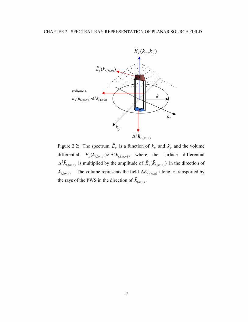
2.2 The spectrum xE is a function of xk and yk and volume
differential 2,( , ) ,( , )( )x t m n t m nE ×Δk k , where the surface
differential 2,( , )t m nΔ k is multiplied by the amplitude of ,( , )( )x t m nE k
in the direction of ,( , )t m nk . The volume represents the field ,( , )x m nEΔ along x transported by the rays of
the PWS in the direction of ( , )m nk . ………………………………… 17
2.3 The rays of the PWS arrive at point P(x,y,z) in direction k of the middle ray and surrounded by four vectors
1 2 3 4, , , and k k k k in the spatial and spectral domains. .…………….... 18
2.4 (a) A PWS ray arrives at point P(x,y,z) in direction ,m nk , in 3-D. And (b) ray in spectral domain kxkyk. ……………………………….. 22
2.5 The transverse vector components 1,( , ) , m nk 2,( , ) ,m nk 3,( , ) m nk
4,( , )and m nk and the surface differential 2,( , )t m nd k covered
by the vectors in the x yk k -plane. The transverse component
,( , )t m nk is placed at the center of 2,( , )t m nd k . ……………………….... 24
2.6 A ray of PWS arrives at point P(x,y,z) in the direction ,m nk in free-space xyz and also in spectral domain kxkykz.. ………………... 25 3.1 The geometry of the hyper-hemispherical lens for tracing
the backward launched ray in the φ plane. …………………….….. 31 3.2 Rays are launched backward from the observation point (θ, 0φ = ) to the source plane, where each ray samples the spectral domain of the source. ………………………………………. 33

xii
3.3 The 12,ˆ Mz TPR contour in the ( , )θ φ plane.
In the proposed implementation in Matlab, the matrix is divided into
12, , lnˆ cyMz and 12, ,ˆ sphMz , the cylindrical
and spherical parts. For the matrix representation of SRT, all TPR along θ are computed using matrix operations at once. ….… 37
3.4 The matrix 2,ˆiMz TPR in the ( , )θ φ plane and the 2,ˆ
im Mz vector, which is the middle ray of the matrix. ………………………. 38
3.5 The geometry of the 5 mm radius (7.3λ) hemispherical lens. ………. 40
3.6 The E-plane far-field, Ex radiation pattern in dB and phase of electric field obtained using SRT for the R = 5 mm hemispherical lens with 3.8rε = . ………………….. 41
3.7 The E-plane far-field, Ex radiation pattern in dB and phase of electric field obtained using SRT and GO for the R = 25 mm hyper-hemispherical silica lens (d = 12.84 mm)…. 42
3.8 The converges of the magnitdude of far-field Ex as the ray density is increased. ………………………………………. 43
3.9 The converges of the phase of far-field Ex as the ray density is increased. …………………………………………. 44
3.10 The Integrated lens antenna with structures that are analyzed by rigorous numerical methods surrounded by virtual boxes. ……… 46
3.11 The planar layered structure used to find the initial near-field distribution of the THz or millimeter-wave planar antenna that radiates to an electrically large dielectric.
The substrate is LTG-GaAs and the dielectric half-space is Silicon ( 11.9rε = ). ……………………………………………...….. 48
3.12 Schematic of HSRT algorithm process. …………………………….. 49
3.13 The geometry of the 5 mm radius hyper-hemispherical lens backed by bow-tie antenna (a) in 3D space and (b) the fabricated THz bow-tie antenna on LTG-GaAs shown from the back. ………………….…………………………… 52
3.14 The (a) complex magnitude of Ex Electric field distribution over the aperture plane z = -d of the bow-tie antenna with CPS line feed simulated at 100 GHz and (b) the E-plane far-field radiation pattern in polar coordinates for the bow-tie in dielectric half-space. ………………………….… 55

xiii
3.15 The total electric near-field distribution for the bow-tie antenna feed by a discrete port and simulated using FEKO MoM. …. 56
3.16 The (a) E-plane far-field, Ex radiation pattern for the bow-tie antenna backed by Si hyper-hemispherical lens with FEM-SRT and HFSS responses, and (b) radiation pattern of total E field in polar coordinates, from HFSS. …………………………………………………………. 57
3.17 The E-plane far-field total electric field radiation pattern in dB of electric field obtained using MoM-SRT for the R = 5 mm hyper-hemispherical silicon lens ( 11.9rε = , d = 0.84 mm). The simulation includes application of MoM-SRT hybrid approach for different reflection orders and the simulation results for the Physical Optics (PO), and Method of Moment (MoM). …………………………………….. 58
3.18 The geometry and (a) schematic diagram of the lens antenna system along its coordinates, and (b) the FEKO mesh for the 5 mm radius hyper-hemispherical lens backed by
dipole antenna and Si piece. ………………………………...………. 62
3.19 (a) Die photo of the fabricated VCO integrated with the
on-chip dipole antenna and (b) Transmitter head consists
of Si lens and carrier PCB attached to a XY linear
stage for precise positioning. ………………………………………... 63
3.20 The spectrum (a) ( , )x x yE k k and (b) ( , )y x yE k k of near-field for the THz dipole antenna backed by Silicon lens. The effect of the lens is included in the near-field distribution. ……………….. 64
3.21 The Normalized H-plane far-field total electric field radiation pattern in dB of electric field obtained using Hybrid MoM-SRT for the R = 5 mm hyper-hemispherical silicon lens ( 311.9, 5 10 S/mrε σ −= = × , d = 0.84 mm). Radiation pattern measured at 181 GHz and θ=90° plane (Vcc=2.5 V, Vctr=1.6 V). The HSRT ray density was set as 600 along ϕ x 600 along θ for total of 360,000 rays launched. ………………………………….. 65
3.22 Simulated 3D plot of the THz dipole antenna gain (a) with and (b) without the Si lens and chip carrier obtained using FEKO. ……………………………………………… 66

xiv
3.23 (a) A schematic of double-slot antenna printed at the back of hyper-hemispherical lens and (b) the FEKO mesh for the double-slot antenna backed by the lens. ….……………………… 68
3.24 (a) E-plane (ϕ = 0ᴼ) far-field total electric field radiation patterns in dB of double-slot antenna with lens and (b) E-plane for angles between -20ᴼ to 20ᴼ of electric field obtained using FEM-SRT for the R = 5 mm hyper-hemispherical silica lens ( 3.8rε = , d = 2.565 mm). .……………………………….. 70
3.25 (a) H-plane (ϕ = 90ᴼ) far-field total electric field radiation patterns in dB of double-slot antenna with lens and (b) H-plane for angles between -20ᴼ to 20ᴼ of electric field obtained using FEM-SRT for the R = 5 mm hyper-hemispherical silica lens ( 3.8rε = , d = 2.565 mm). .……………………………… 71
3.26 The convergence of the (a) total far-field E-field amplitude and (b) the difference between successive E-field amplitudes calculated by HSRT method at observation angle ( 0.05 , 0θ φ= = ) for slot antenna on the R = 5 mm hyper-hemispherical silica lens. …… 72
3.27 Experimental setup for Pulsed/CW measurement of THz link….……. 74
3.28 A large-aperture dc-biased terahertz photoconductive antenna placed on a hyper-hemispherical silicon lens excited by a short pulse laser. V is the applied bias voltage and sJ is the induced surface current. ……………………………………………… 74
3.29 The pulse from large aperture dipole antenna in time domain………... 76
3.30 The spectrum of the pulse from large aperture dipole antenna in the frequency domain. …………………………...... 77
3.31 The phase in angles of the signal for the range from 87.90 GHz
to 0.9 THz of the pulse from large aperture dipole antenna. ………… 77
3.32 The far-field Ex electric field in the time domain at an observation point ( , , ) (61 ,0 ,0 )r cmθ φ = due to large-aperture dc-biased terahertz photoconductive antenna placed on a hyper-hemispherical silicon lens excited by a short pulse laser. …… 81
3.33 The far-field Ex electric field in the time domain at an observation point ( , , ) (61 , 20 ,0 )r cmθ φ = due to large-aperture dc-biased terahertz photoconductive antenna placed on a hyper-hemispherical silicon lens excited by a short pulse laser. …… 82

xv
3.34 The E-plane far-field, Ex, radiation pattern in dB and phase of electric field obtained using SRT for the R = 5 mm Si ( 11.9rε = ) hemispherical lens backed by large-aperture dc-biased terahertz photoconductive antenna at 87.9336 GHz. ……… 83
3.35 The E-plane far-field, Ex, radiation pattern in dB and phase of electric field obtained using SRT for the R = 5 mm Si ( 11.9rε = ) hemispherical lens backed by large-aperture dc-biased terahertz photoconductive antenna at 102.5892 GHz. ...…… 83
3.36 The E-plane far-field, Ex, radiation pattern in dB and phase of electric field obtained using SRT for the R = 5 mm hemispherical lens with 11.9rε = for large-aperture (4 mm × 1 mm) dc-biased terahertz photoconductive antenna at 87.9336 GHz. …..…... 84
3.37 The E-plane far-field, Ex, radiation pattern in dB and phase of electric field obtained using SRT for the R = 5 mm hemispherical lens with 11.9rε = for large-aperture (4 mm × 1 mm) dc-biased terahertz photoconductive antenna at 102.5892 GHz. ..…..... 84
3.38 The E-plane far-field, Ex in the time domain obtained using SRT for the R = 5 mm hemispherical lens with 11.9rε = for large-aperture (4 mm × 1 mm) dc-biased terahertz photoconductive antenna at different angles of observation……....….. 85
3.39 The simulated directivity vs. frequency for the E-plane far-field….….. 85
4.1 Schematic of a dipole antenna connected to a VCO via transmission line. ……………………………………………………... 88
4.2 Simulated input return loss of the planar dipole on half-space silicon. …………………………………………………….. 89
4.3 (a) Schematic diagram of the quasi-optical setup and (b) Quasi-optical test bench. …………………………………...……... 91
4.4 (a) Schematic diagram of the superheterodyne setup and (b) Superheterodyne test bench. ……………………………………… 93
4.5 Measured spectrum of the 180-GHz VCO. The conversion loss of the harmonic mixer is included in the power reading. ...……… 94
5.1 (a) Simplified Schematic layout of the slab sample, source and detector for transmission mode measurements. ………….……..... 98
5.2 (a) Schematic layout of the quasioptical Spectrometer for transmission mode measurements. The components are number and described below, (b) the sample holder on a motor controlled by LabView, and (c) the BWO. …………………… 100
xvi
5.3 Aluminium plates precisely cut to place biological tissue sample size for millimeter and sub-millimeter wave quasi-optical spectroscopy measurements. ………………………………………... 101
5.4 The tooth samples, (a) Enamel sample, (b) Root, (c) dental carries sample. ……………………………………………………….. 102
5.5 The transmission coefficient for Enamel sample. …………………… 103
5.6 The transmission coefficient for (a) dentine from root and (b) dental caries. …………………………………………………….. 104
5.7 The measured attenuation coefficient of enamel. The values shown are within ± 7 dB/cm. ……………...………….…. 105
5.8 The attenuation coefficient of the root dentine. …………………….. 105
5.9 The attenuation coefficient for the dental caries sample. ……...……. 106
5.10 The THz CW imaging measurement setup available at MISL. ……... 109
5.11 The measured Point Spread Function along horizontal x-axis at 840 GHz. .………………………………………………..... 110
5.12 The THz image of cross-section of tooth shown at 840 GHz based on transmitted power, and the signal strength measured in volts and (b) a visible image of the cross-section of tooth along side the corresponding THz image. ………………………………..... 111
5.13 Measured (a) intensity of focused beam, and (b) deconvolved beam profile of THz source in free-space. ………………………….. 114
5.14 Experimental setup for THz Propagation through a cylinder. ………. 116
5.15 Measured deconvolved beam profile with and without sample in μW. ……………………………………………… 116
5.16 The THz CW imaging of Polyethylene cylinder. …………………… 117
5.17 The THz image of Polyethylene cylinder. …………………………... 117
5.18 The geometry of cylindrical structure and SRT backward launched rays that hit the cylinder in the xy-plane is shown. Here the x = 0 is source plane and x = 14 mm is the observation plane. ……………... 121
5.19 The |Ez| total electric field shown is obtained from 2D TLM simulation for Gaussian beam propagation through a lossless 2D cylinder with beam width of 2λ or w0=λ. The cylinder has R=3.5 mm ≈ 10λ and the source is 3.5 mm from the cylinder. ………………………………….…….. 122
5.20 The (a) magnitude and (b) phase of Ez obtained from 2D SRT, 2D TLM and 2D FDTD simulations of Gaussian beam propagation

xvii
through a 2D cylinder. The location of observation is 14 mm from the source. …………………………………………………………… 123
5.21 The magnitude of the total electric field Ez obtained after 2D TLM simulation for Gaussian beam propagation, w0=λ, through a 7 mm diameter cylinder with a circular hole with diameter of 2 mm at center. ………………………………………………………………. 124
5.22 The (a) magnitude of Ez obtained from 2D TLM simulation for Gaussian beam propagation,w0=λ, through a lossy polyethylene cylinder (εr = 2.3075, σ = 0.01 S/m). (b) The 2D TLM lossy vs. lossless case at x = 11 mm. …………….. 125
5.23 The (a) dielectric profile of the structure to image and (b) the magnitude of Ez obtained from 2D TLM simulation for Gaussian beam propagation, w0=λ, through a cylinder with a circular hole with diameter of 2.72 mm and elliptical hole with diameter of 1.6 mm along x and 4.16 mm along y. ………………….. 127

xviii
List of Abbreviations FEM Finite Element Method
FDTD Finite Difference Time Domain
GO Geometrical Optics
GBT Gaussian Beam Tracing
GTD Geometrical Theory of Diffraction
MoM Method of Moments
PO Physical Optics
PWS Plane Wave Spectrum
SRT Spectral Ray Tracing
HSRT Hybrid Spectral Ray Tracing
UAT Uniform Asymptotic Theory
UTD Uniform Theory of Diffraction
STD Spectral Theory of Diffraction
TPR Tube of Paraxial Rays
1
CHAPTER 1
Introduction
1.1 Why Explore The Terahertz Frequency Range?
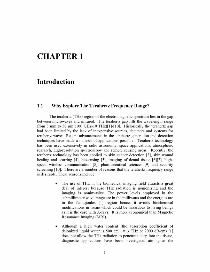
The terahertz (THz) region of the electromagnetic spectrum lies in the gap between microwaves and infrared. The terahertz gap fills the wavelength range from 3 mm to 30 μm (100 GHz-10 THz)[1]-[10]. Historically the terahertz gap had been limited by the lack of inexpensive sources, detectors and systems for terahertz waves. Recent advancements in the terahertz generation and detection techniques have made a number of applications possible. Terahertz technology has been used extensively in radio astronomy, space applications, atmospheric research, high-resolution spectroscopy and remote sensing areas. Recently, the terahertz technology has been applied to skin cancer detection [3], skin wound healing and scarring [4], biosensing [5], imaging of dental tissue [6][7], high-speed wireless communication [8], pharmaceutical sciences [9] and security screening [10]. There are a number of reasons that the terahertz frequency range is desirable. These reasons include:
• The use of THz in the biomedical imaging field attracts a great deal of interest because THz radiation is nonionizing and the imaging is noninvasive. The power levels employed in the submillimeter wave range are in the milliwatts and the energies are in the femtojoules [1] region hence, it avoids biochemical modifications in tissue which could be hazardous to living beings as it is the case with X-rays. It is more economical than Magnetic Resonance Imaging (MRI).
• Although a high water content (the absorption coefficient of deionized liquid water is 500 cm-1 at 3 THz or 2000 dB/cm) [1] does not allow the THz radiation to penetrate deep into the tissue, diagnostic applications have been investigated aiming at the

CHAPTER 1 INTRODUCTION
2
identification of skin cancer, and the detection of pre-caries modifications of the teeth.
• THz Pulse Imaging (TPI) has been used to create an image of a human premolar where the enamel and dentine layers were identified using the change in the refractive index [7]. Other than being a nonionizing imaging modality, TPI has an advantage compared to X-ray imaging and MRI due to its ability to perform spectroscopic measurements, time-of-flight and average absorption information at each pixel in an image.
• The wavelength regime is appropriate for imaging since the diffraction limited spot size is consistent (1.22λ0=366 μm at 1 THz) with the resolution of a decent computer monitor (~70 dots/in.)
• At THz frequencies, the terahertz signals can pass through tissue with only Mie or Tyndall scattering (proportional to f 2) rather than a much stronger Rayleigh scattering (proportional to f 4) that dominates optical and IR ranges.
• The energy levels in the THz range are consistent with in the discrete molecular vibrational modes in liquids, proteins and solids [1]. Astronomers, space scientists and molecular chemists have mapped thermal emission lines for a wide variety of light-weight molecules, since much spectroscopy information is found in this THz region of the EM spectrum. Since the terahertz signal is remote and nondestructive, this is a fast and powerful method for label-free DNA sequencing using change in the index of the refraction when the DNA in the solution is hybridized [11].
• In the pharmaceutical industry, applications of THz include non-destructive and non-invasive tablet coating analysis and drug counterfeiting detection.
• The atmospheric opacity limits radar and communications applications at terahertz frequencies, but wireless indoor communication with data rates in the tens of gigabits per second are possible if small and efficient THz transmitters are developed. At the THz range, a secure communication with attenuation outside the target area is promising with small antenna sizes integrated on a THz chip to take advantage of large bandwidth of the THz carriers.
CHAPTER 1 INTRODUCTION
3
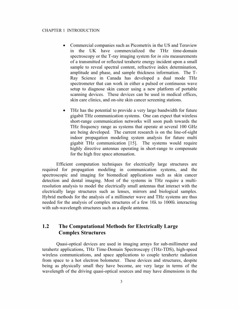
• Commercial companies such as Picometrix in the US and Teraview in the UK have commercialized the THz time-domain spectroscopy or the T-ray imaging system for in situ measurements of a transmitted or reflected terahertz energy incident upon a small sample to reveal spectral content, refractive index determination, amplitude and phase, and sample thickness information. The T-Ray Science in Canada has developed a dual mode THz spectrometer that can work in either a pulsed or continuous wave setup to diagnose skin cancer using a new platform of portable scanning devices. These devices can be used in medical offices, skin care clinics, and on-site skin cancer screening stations.
• THz has the potential to provide a very large bandwidth for future gigabit THz communication systems. One can expect that wireless short-range communication networks will soon push towards the THz frequency range as systems that operate at several 100 GHz are being developed. The current research is on the line-of-sight indoor propagation modeling system analysis for future multi gigabit THz communication [15]. The systems would require highly directive antennas operating in short-range to compensate for the high free space attenuation.
Efficient computation techniques for electrically large structures are required for propagation modeling in communication systems, and the spectroscopic and imaging for biomedical applications such as skin cancer detection and dental imaging. Most of the systems in THz require a multi-resolution analysis to model the electrically small antennas that interact with the electrically large structures such as lenses, mirrors and biological samples. Hybrid methods for the analysis of a millimeter wave and THz systems are thus needed for the analysis of complex structures of a few 10λ to 1000λ interacting with sub-wavelength structures such as a dipole antenna.
1.2 The Computational Methods for Electrically Large Complex Structures
Quasi-optical devices are used in imaging arrays for sub-millimeter and
terahertz applications, THz Time-Domain Spectroscopy (THz-TDS), high-speed wireless communications, and space applications to couple terahertz radiation from space to a hot electron bolometer. These devices and structures, despite being as physically small they have become, are very large in terms of the wavelength of the driving quasi-optical sources and may have dimensions in the
CHAPTER 1 INTRODUCTION
4
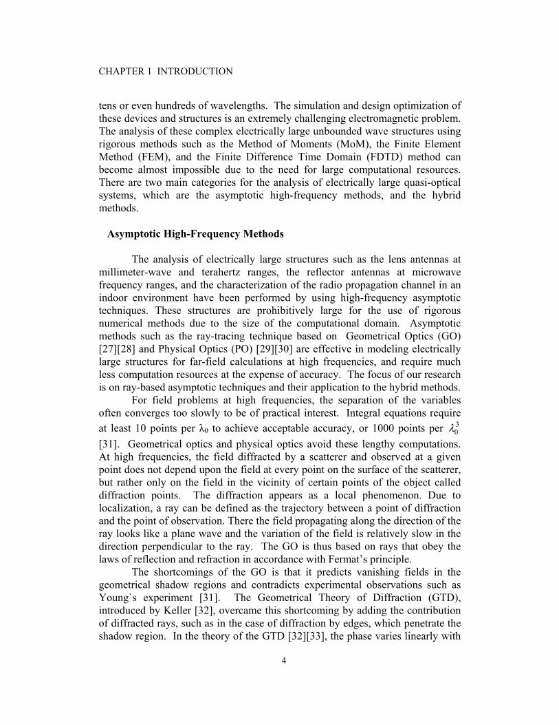
tens or even hundreds of wavelengths. The simulation and design optimization of these devices and structures is an extremely challenging electromagnetic problem. The analysis of these complex electrically large unbounded wave structures using rigorous methods such as the Method of Moments (MoM), the Finite Element Method (FEM), and the Finite Difference Time Domain (FDTD) method can become almost impossible due to the need for large computational resources. There are two main categories for the analysis of electrically large quasi-optical systems, which are the asymptotic high-frequency methods, and the hybrid methods.
Asymptotic High-Frequency Methods The analysis of electrically large structures such as the lens antennas at
millimeter-wave and terahertz ranges, the reflector antennas at microwave frequency ranges, and the characterization of the radio propagation channel in an indoor environment have been performed by using high-frequency asymptotic techniques. These structures are prohibitively large for the use of rigorous numerical methods due to the size of the computational domain. Asymptotic methods such as the ray-tracing technique based on Geometrical Optics (GO) [27][28] and Physical Optics (PO) [29][30] are effective in modeling electrically large structures for far-field calculations at high frequencies, and require much less computation resources at the expense of accuracy. The focus of our research is on ray-based asymptotic techniques and their application to the hybrid methods.
For field problems at high frequencies, the separation of the variables often converges too slowly to be of practical interest. Integral equations require at least 10 points per λ0 to achieve acceptable accuracy, or 1000 points per 3
0λ [31]. Geometrical optics and physical optics avoid these lengthy computations. At high frequencies, the field diffracted by a scatterer and observed at a given point does not depend upon the field at every point on the surface of the scatterer, but rather only on the field in the vicinity of certain points of the object called diffraction points. The diffraction appears as a local phenomenon. Due to localization, a ray can be defined as the trajectory between a point of diffraction and the point of observation. There the field propagating along the direction of the ray looks like a plane wave and the variation of the field is relatively slow in the direction perpendicular to the ray. The GO is thus based on rays that obey the laws of reflection and refraction in accordance with Fermat’s principle.
The shortcomings of the GO is that it predicts vanishing fields in the geometrical shadow regions and contradicts experimental observations such as Young`s experiment [31]. The Geometrical Theory of Diffraction (GTD), introduced by Keller [32], overcame this shortcoming by adding the contribution of diffracted rays, such as in the case of diffraction by edges, which penetrate the shadow region. In the theory of the GTD [32][33], the phase varies linearly with

CHAPTER 1 INTRODUCTION
5
the travelling distance along a ray and the power is converged in a tube of rays. Keller [32] used an exact solution of scattering from simple shapes, known as canonical problems, to derive GTD expressions for diffracted fields. Since the diffracted field carried by the ray depends on the local properties of the incident field and local interaction with the object, the original scatterer is replaced with a canonical object whose local geometrical and physical properties are identical to those of the original scatterer. Examples of canonical problems include the plane wave reflection and refraction at an infinite planar dielectric surface, the half-plane and wedge solutions, and scattering by a circular cylinder, and sphere. The key step in the GTD is to find the rays that are predominant contributors to the diffracted field and to evaluate the field along each ray using the GTD diffraction coefficients. Diffraction coefficients derived from the canonical problem are multiplied with the incident ray at the point of diffraction to produce the initial value of the field on the diffracted ray. The GTD diffraction coefficients are non-uniform and invalid in the transition region adjacent to the shadow boundary where the diffracted field plays a significant role in edge and convex surface diffraction. The fields computed by the GTD are infinite on caustics and discontinuous on the light-shadow boundaries.
The Uniform Asymptotic Theory (UAT) [35] and Uniform Theory of Diffraction (UTD) [36] were developed to resolve the aforementioned issues with the GTD. The UTD departs from the pure ray optical field approximation to correct the shortcoming of the GTD within the shadow boundary transition region and reduces the GTD outside to this transition region. Kouyoumjan and Pathak [36] begin with an ansatz for the diffracted field based on the uniform solution of the wedge with the planar faces using the Pauli-Clemmow method. By considering the wedge, which is locally tangent to the wedge with curved faces at the diffraction point, the divergence factor of the diffracted wave is extended to the case of a curved edge that is illuminated by a local planar wave. The total field is the sum of the incident and reflected GO fields, and the field diffracted by the edges. In order for the diffracted field to compensate the jump discontinuity of the incident and reflected fields across their shadow boundaries, the arguments of the Fresnel functions in the expressions of the diffraction coefficients are modified to satisfy the continuity of the total field across the shadow boundary. High frequency diffraction by the regular convex Perfect Electric Conductors (PEC) using different ansatz have been extensively researched by Pathak et al. [38][40] and Mittra and Safavi-Naeini [39].
Lee and Deschamps [37] derived the UAT solution constructed from the uniform solution of the wedge with planar faces by using the Van de Waerden method. They introduced detour parameters corresponding to the detour that the phase makes along the path followed by the diffracted ray. The uniform asymptotic solution of the total field is obtained by extending the divergence factor of the diffracted wave to the case of a curved edge that is illuminated by a locally plane wave, and by generalizing the detour parameters to the 3D

CHAPTER 1 INTRODUCTION
6
geometries of the wedge and incident wave. The diffraction coefficients are non-uniform Keller coefficients, and the reflected field is an extension of the GO through the continuity of the phase and the amplitude. As the detour parameters approach zero, the singularity of the Fresnel functions evaluated at the detour parameters are compensated by the corresponding singularities of the diffraction coefficients in the neighborhood of the direct field’s the shadow boundary for the continuity of the total field. The uniform asymptotic solution is continuous across both the incident and reflected shadow boundaries and becomes identical to the non-uniform solution far from the shadow boundaries. For the UAT solution, the continuity of the derivatives of the field is satisfied unlike the UTD, where a slope diffraction coefficient has to be introduced as a corrective term [41]. The UAT yields an asymptotic expansion that includes the terms O(k-1/2) since the UAT solution finds a term that depends upon the derivative of the reflected field in the direction normal to the shadow boundary [42]. The UTD with slope diffraction coefficients of the incident and reflected field can obtain a solution equivalent to the UAT. The UTD is more convenient than the UAT since it is neither necessary to extend the surface nor find fictitious rays with the UTD.
Hybrid Methods
Modern communication systems typically utilize electrically small
antennas mounted on a comparatively electrically large platform such as a car or an airplane. From modeling THz integrated antennas, quasi-optical system, and large microwave and millimeter wave antennas to accurately modeling an indoor millimeter wave and THz propagation close to the complex discontinuities, the hybrid methods that combine rigorous numerical methods such as the Method of Moments (MoM), Finite Element Method (FEM), and/or Finite-Difference Time-Domain (FDTD) with asymptotic methods are needed to model the entire structure. A number of hybrid methods have been developed over the years to tackle this class of problems, where the complex PEC or dielectric structures have a pronounced effect on the electrical characteristics such as the radiation patterns.
Hybrid methods are broadly categorized as either ray-based or current-based techniques. Ray-based techniques such as the MoM-GTD[43], [44] provide a considerable speed advantage, but are quite difficult to implement for an arbitrary and complex object. In contrast, the current-based methods such as the MoM-PO[45][46] and the FEM-PTD [47], that attempt to determine the equivalent surface currents that represent an object are inherently capable of modeling irregular geometries given a good approximation of the current. A hybrid method based on the combination of the ray tracing and the FDTD method was developed for accurate modeling of the indoor radio wave propagation [48],[49]. The technique uses ray tracing to analyze the wide areas and FDTD to model areas close to complex discontinuities., where it incorporates the reflection, refraction and diffraction by solving Maxwell’s equation in the time-domain. The
CHAPTER 1 INTRODUCTION
7
technique has also been applied using the FDTD method to study the effects of inhomogeneities inside walls and small indoor structural features.
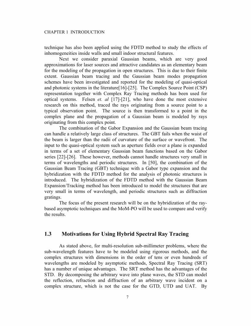
Next we consider paraxial Gaussian beams, which are very good approximations for laser sources and attractive candidates as an elementary beam for the modeling of the propagation in open structures. This is due to their finite extent. Gaussian beam tracing and the Gaussian beam modes propagation schemes have been investigated and reported for the modeling of quasi-optical and photonic systems in the literature[16]-[25]. The Complex Source Point (CSP) representation together with Complex Ray Tracing methods has been used for optical systems. Felsen et. al [17]-[21], who have done the most extensive research on this method, traced the rays originating from a source point to a typical observation point. The source is then transformed to a point in the complex plane and the propagation of a Gaussian beam is modeled by rays originating from this complex point.
The combination of the Gabor Expansion and the Gaussian beam tracing can handle a relatively large class of structures. The GBT fails when the waist of the beam is larger than the radii of curvature of the surface or wavefront. The input to the quasi-optical system such as aperture fields over a plane is expanded in terms of a set of elementary Gaussian beam functions based on the Gabor series [22]-[26]. These however, methods cannot handle structures very small in terms of wavelengths and periodic structures. In [50], the combination of the Gaussian Beam Tracing (GBT) technique with a Gabor type expansion and the hybridization with the FDTD method for the analysis of photonic structures is introduced. The hybridization of the FDTD method with the Gaussian Beam Expansion/Tracking method has been introduced to model the structures that are very small in terms of wavelength, and periodic structures such as diffraction gratings.
The focus of the present research will be on the hybridization of the ray-based asymptotic techniques and the MoM-PO will be used to compare and verify the results.
1.3 Motivations for Using Hybrid Spectral Ray Tracing As stated above, for multi-resolution sub-millimeter problems, where the
sub-wavelength features have to be modeled using rigorous methods, and the complex structures with dimensions in the order of tens or even hundreds of wavelengths are modeled by asymptotic methods, Spectral Ray Tracing (SRT) has a number of unique advantages. The SRT method has the advantages of the STD. By decomposing the arbitrary wave into plane waves, the STD can model the reflection, refraction and diffraction of an arbitrary wave incident on a complex structure, which is not the case for the GTD, UTD and UAT. By
CHAPTER 1 INTRODUCTION
8
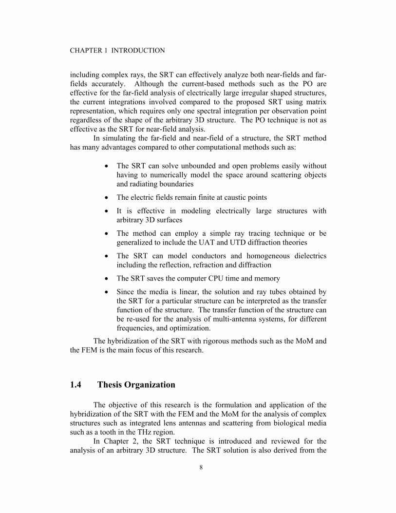
including complex rays, the SRT can effectively analyze both near-fields and far-fields accurately. Although the current-based methods such as the PO are effective for the far-field analysis of electrically large irregular shaped structures, the current integrations involved compared to the proposed SRT using matrix representation, which requires only one spectral integration per observation point regardless of the shape of the arbitrary 3D structure. The PO technique is not as effective as the SRT for near-field analysis.
In simulating the far-field and near-field of a structure, the SRT method has many advantages compared to other computational methods such as:
• The SRT can solve unbounded and open problems easily without
having to numerically model the space around scattering objects and radiating boundaries
• The electric fields remain finite at caustic points
• It is effective in modeling electrically large structures with arbitrary 3D surfaces
• The method can employ a simple ray tracing technique or be generalized to include the UAT and UTD diffraction theories
• The SRT can model conductors and homogeneous dielectrics including the reflection, refraction and diffraction
• The SRT saves the computer CPU time and memory
• Since the media is linear, the solution and ray tubes obtained by the SRT for a particular structure can be interpreted as the transfer function of the structure. The transfer function of the structure can be re-used for the analysis of multi-antenna systems, for different frequencies, and optimization.
The hybridization of the SRT with rigorous methods such as the MoM and the FEM is the main focus of this research.
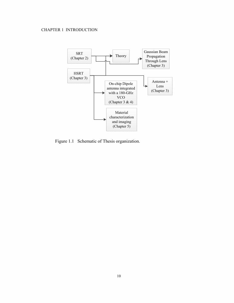
1.4 Thesis Organization
The objective of this research is the formulation and application of the hybridization of the SRT with the FEM and the MoM for the analysis of complex structures such as integrated lens antennas and scattering from biological media such as a tooth in the THz region.
In Chapter 2, the SRT technique is introduced and reviewed for the analysis of an arbitrary 3D structure. The SRT solution is also derived from the
CHAPTER 1 INTRODUCTION
9
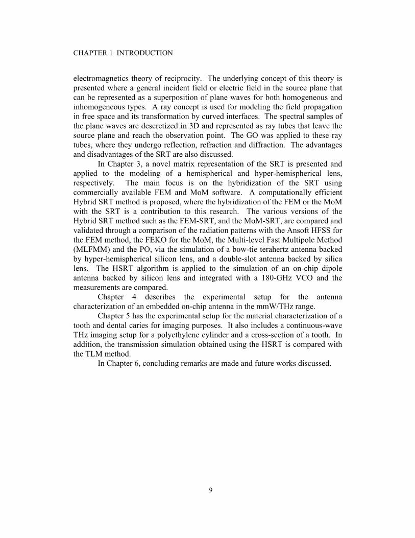
electromagnetics theory of reciprocity. The underlying concept of this theory is presented where a general incident field or electric field in the source plane that can be represented as a superposition of plane waves for both homogeneous and inhomogeneous types. A ray concept is used for modeling the field propagation in free space and its transformation by curved interfaces. The spectral samples of the plane waves are descretized in 3D and represented as ray tubes that leave the source plane and reach the observation point. The GO was applied to these ray tubes, where they undergo reflection, refraction and diffraction. The advantages and disadvantages of the SRT are also discussed.
In Chapter 3, a novel matrix representation of the SRT is presented and applied to the modeling of a hemispherical and hyper-hemispherical lens, respectively. The main focus is on the hybridization of the SRT using commercially available FEM and MoM software. A computationally efficient Hybrid SRT method is proposed, where the hybridization of the FEM or the MoM with the SRT is a contribution to this research. The various versions of the Hybrid SRT method such as the FEM-SRT, and the MoM-SRT, are compared and validated through a comparison of the radiation patterns with the Ansoft HFSS for the FEM method, the FEKO for the MoM, the Multi-level Fast Multipole Method (MLFMM) and the PO, via the simulation of a bow-tie terahertz antenna backed by hyper-hemispherical silicon lens, and a double-slot antenna backed by silica lens. The HSRT algorithm is applied to the simulation of an on-chip dipole antenna backed by silicon lens and integrated with a 180-GHz VCO and the measurements are compared.
Chapter 4 describes the experimental setup for the antenna characterization of an embedded on-chip antenna in the mmW/THz range.
Chapter 5 has the experimental setup for the material characterization of a tooth and dental caries for imaging purposes. It also includes a continuous-wave THz imaging setup for a polyethylene cylinder and a cross-section of a tooth. In addition, the transmission simulation obtained using the HSRT is compared with the TLM method.
In Chapter 6, concluding remarks are made and future works discussed.
CHAPTER 1 INTRODUCTION
10
SRT(Chapter 2)
HSRT(Chapter 3)
On-chip Dipole antenna integrated with a 180-GHz
VCO (Chapter 3 & 4)
Material characterization
and imaging (Chapter 5)
TheoryGaussian Beam
Propagation Through Lens
(Chapter 3)
Antenna + Lens
(Chapter 3)
Figure 1.1 Schematic of Thesis organization.

11
CHAPTER 2
The Spectral Ray Representation of a
Planar Source Field
2.1 Introduction
The analysis of complex electrically large structures using the Method of Moments (MoM), the Finite Element Method (FEM), and the Finite Difference Time Domain (FDTD) method can become prohibitive due to the need for large computational resources. The asymptotic methods discussed in Chapter 1 require much less computation resources at the expense of accuracy and are effective in modeling electrically large structures for far-field calculations at high frequencies.
As a general asymptotic formulation of the EM scattering by a complex object, Spectral Ray Tracing (SRT)[60]-[62] was first proposed for modeling quasi-optical systems. The SRT is an alternative for a reliable and accurate computation of the electromagnetic field in the near-field and far-field regions of large structures that use much less computational resources compared with numerical methods. In this chapter, for the first time the SRT is derived from the Electromagnetics Reciprocity theory and Parseval’s theorem. The SRT is based on the Spectral Theory of Diffraction (STD) [31] introduced by Mittra et al.. The underlying concept of this theory is that a general incident field or electric field in the source plane can be represented as a superposition of the plane waves of both the homogeneous and inhomogeneous type. A ray representation is used for modeling the field propagation in free space and the reflection, refraction, and diffraction by the curved interfaces. The incident field spectrum is sampled by plane wave rays, which will form tubes that leave the source plane and reach the observation point. The GO, GTD and/or more advanced versions of the diffraction theories such as the UTD are applied to these rays, where they undergo reflection, refraction and diffraction. For the transmission through an interface, the transmitted field is approximated by components parallel and perpendicular to the incident plane, to the product of the Fresnel transmission coefficient and a divergence factor.

CHAPTER 2 SPECTRAL RAY REPRESENTATION OF PLANAR SOURCE FIELD
12
The spectral ray representation of the planar source field is given in Section 2.2, followed by the derivation of the SRT solution in Section 2.3. The discretization of the Plane Wave Spectrum (PWS) integrals in 3D is given in Section 2.4, and finally the advantages and disadvantages of the SRT discussed in Section 2.5.
2.2 The Foundation of SRT
In this section, we represent the field radiated from a known planar source at z = 0 in terms of spectral rays (see Fig. 2.1(a)). Suppose the tangential electric fields ( , ,0), ( , ,0)x yE x y E x y at the source plane are given. The electric field at any point in the half-space z > 0 is calculated using the known field in the plane z = 0, which serves as a boundary condition. Through the Fourier transform, F , of the electric field over the plane z = 0, ( , )x x yE k k and ( , )y x yE k k represent the Fourier transform of ( , ,0)xE x y and ( , ,0)yE x y , and we are able to write [34]
Omitting the factor j te ω , the electric field components Ex and Ey at point P(x,y, z > 0) are found as a plane-wave superposition
where ( , , )x y zk k k=k is the wave vector with 2 2 2 2x y zk k k k π
λ= + + = =k and
λ is the wavelength of the propagating field.
( )2
( , ) [ ( , ,0)]
1 ( , ,0)4
x y
x x y x
j k x k yx
E k k F E x y
E x y e dxdyπ
+∞ +∞ +
−∞ −∞
=
= ∫ ∫.
(2.1)
( )2
( , ) [ ( , ,0)]
1 ( , ,0)4
x y
y x y y
j k x k yy
E k k F E x y
E x y e dxdyπ
+∞ +∞ +
−∞ −∞
=
= ∫ ∫.
(2.2)
1
( )
( , , ) [ ( , ) ]
( , )
z
x y z
jk zx x x y
j k x k y k zx x y x y
E x y z F E k k e
E k k e dk dk
−−
+∞ +∞ − + +
−∞ −∞
=
= ∫ ∫.
(2.3)
1
( )
( , , ) [ ( , ) ]
( , )
z
x y z
jk zy y x y
j k x k y k zy x y x y
E x y z F E k k e
E k k e dk dk
−−
+∞ +∞ − + +
−∞ −∞
=
= ∫ ∫.
(2.4)
CHAPTER 2 SPECTRAL RAY REPRESENTATION OF PLANAR SOURCE FIELD
13
We denote ( , )x x yE k k and ( , )y x yE k k as the x- and y-components respectively, of the electric field’s Plane Wave Spectrum (PWS). Assuming Gauss’ Law holds, once we use Eq. 2.3 and Eq. 2.4 to obtain ( , , )xE x y z and
( , , )yE x y z at point ( , , 0)P x y z > , employing Maxwell’s equations gives the remaining component ( , , )zE x y z , and the components
( , , ), ( , , ) and ( , , )x y zH x y z H x y z H x y z of the magnetic field at the observation
point ( , , 0)P x y z > . Thus, the two scalar angular spectra ( , )x x yE k k and
( , )y x yE k k completely describe the field throughout the half-space z > 0 [34]. The component ( , , )zE x y z is calculated the following way [88]
where
is the PWS of the component along z. To do the numerical calculation, the integral Eq. (2.3), Eq. (2.4) and Eq.
(2.5) have to be discretized. The discretization is introduced using the notion of ray (see Appendix 3).
The objective of the method is to find the field everywhere. For this purpose, we first expand the source field in terms of the rays which are obtained from the discretization of the spectrum of the source. The second step, is tracing the rays from the source to the observation point and the sum contribution of the rays that pass through the observation point. In step two, since it is difficult to determine the rays that reach the observation point, based on reciprocity we launch the rays backward (backward ray launching) from the observation point.
In the next section, we start with the backward wave launching concept.
2.3 Derivation of SRT Solution [96]
The SRT has two main steps. The first step consists of a plane wave
expansion of the known source distribution in free-space, and the second step is the backward ray tracing.
To describe the first step, it is assumed that the equivalent source currents
1
( )
( , , ) [ ( , ) ]
( , )
z
x y z
jk zz z x y
j k x k y k zz x y x y
E x y z F E k k e
E k k e dk dk
−−
+∞ +∞ − + +
−∞ −∞
=
= ∫ ∫.
(2.5)
( , ) ( , )( , ) x x y x y x y y
z x yz
E k k k E k k kE k k
k+
= − . (2.6)
CHAPTER 2 SPECTRAL RAY REPRESENTATION OF PLANAR SOURCE FIELD
14
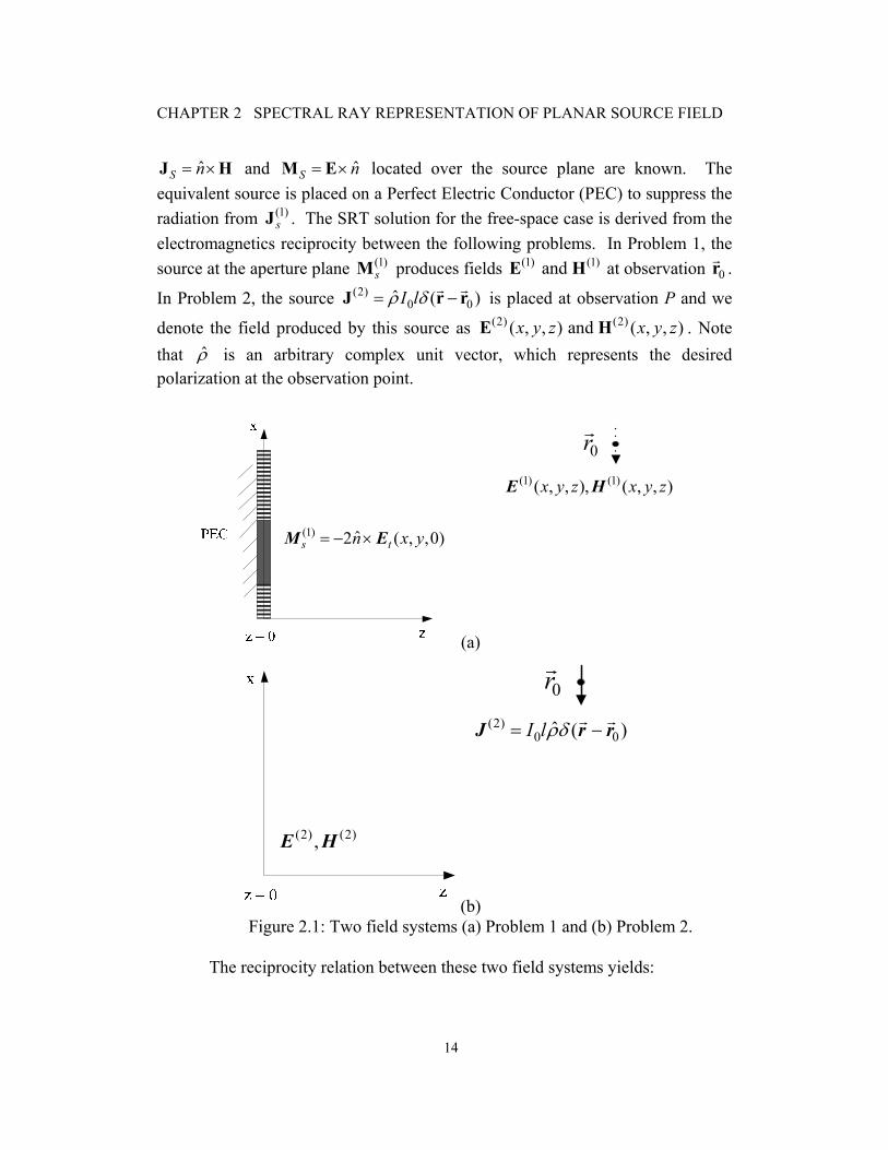
ˆS n= ×J H and ˆS n= ×M E located over the source plane are known. The equivalent source is placed on a Perfect Electric Conductor (PEC) to suppress the radiation from (1)
sJ . The SRT solution for the free-space case is derived from the electromagnetics reciprocity between the following problems. In Problem 1, the source at the aperture plane (1)
sM produces fields (1) (1)and E H at observation 0r .
In Problem 2, the source (2)0 0ˆ ( )I lρ δ= −J r r is placed at observation P and we
denote the field produced by this source as (2) (2)( , , ) and ( , , )x y z x y zE H . Note that ρ is an arbitrary complex unit vector, which represents the desired polarization at the observation point.
(a)
(b) Figure 2.1: Two field systems (a) Problem 1 and (b) Problem 2.
The reciprocity relation between these two field systems yields:
0r(1) (1)( , , ), ( , , )x y z x y zΕ H
(1) ˆ2 ( , ,0)s tn x y= − ×M E
0r(2)
0 0ˆ ( )I lρδ= −J r r
(2) (2),E H

CHAPTER 2 SPECTRAL RAY REPRESENTATION OF PLANAR SOURCE FIELD
15
Since the source is over a planar surface, the L.H.S. of Eq. (2.7) becomes
The R.H.S. of Eq. (2.7) is
The magnetic field in the far-zone produced by an infinitesimal dipole (source in Problem 2) at the observation point is
Substituting Eq. (2.10) into Eq. (2.8) we get [96]
where sin 1θ = (paraxial) and 0R = −r r 2 2 20 0 0( ) ( ) ( )x x y y z z= − + − + − .
Then we directly apply Parseval’s theorem at the source plane to convert Eq. (2.11) to a Fourier domain integral. For this purpose, using the plane wave representation, [29]
one may find the following Fourier transform
at z = 0. Therefore Eq. (2.11) becomes [96]
(2) (1) (1) (2)s
V V
dv dv− =∫∫∫ ∫∫∫H M E Ji i . (2.7)
(2) (1) (2)ˆ(2 ( , ,0))s tV S
dv n x y ds− = ×∫∫∫ ∫∫H M E Hi i . (2.8)
(1) (2) (1) (1)0 0 0 0ˆ ˆ( ) ( )
V V
dv I l dv I lρ δ ρ= − =∫∫∫ ∫∫∫E J E r r E ri . (2.9)
(2) 0ˆ ˆsin4
jkRE jkI leR
θ φ θφη π
−
=H . (2.10)
(1) 00 0
ˆˆ ˆ( ) ( ( , ,0)) sin2
jkR
tS
jkI l eI l n x y dxdyR
ρ φ θπ
−
= ×∫∫E r E i . (2.11)
0 000
( )( )( )
0
1 .2
zyx
jk jk z zjk y yjk x x
x yz
e e e e dk dkj kπ
+∞ +∞− − − −−−
−∞ −∞
=− ∫ ∫
r r
r r (2.12)
0 000
0
zyx
jk jk zjk yjk x
z
e eF e ek
− − −−−
⎧ ⎫⎪ ⎪ =⎨ ⎬−⎪ ⎪⎩ ⎭
r r
r r (2.13)
CHAPTER 2 SPECTRAL RAY REPRESENTATION OF PLANAR SOURCE FIELD
16
where 2 2 2z x yk k k k= − − .
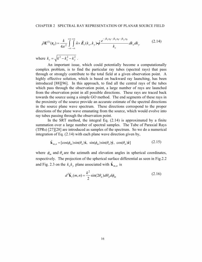
An important issue, which could potentially become a computationally complex problem, is to find the particular ray tubes (spectral rays) that pass through or strongly contribute to the total field at a given observation point. A highly effective solution, which is based on backward ray launching, has been introduced [88][96]. In this approach, to find all the central rays of the tubes which pass through the observation point, a large number of rays are launched from the observation point in all possible directions. These rays are traced back towards the source using a simple GO method. The end segments of these rays in the proximity of the source provide an accurate estimate of the spectral directions in the source plane wave spectrum. These directions correspond to the proper directions of the plane wave emanating from the source, which would evolve into ray tubes passing through the observation point.
In the SRT method, the integral Eq. (2.14) is approximated by a finite summation over a large number of spectral samples. The Tube of Paraxial Rays (TPRs) [27][28] are introduced as samples of the spectrum. So we do a numerical integration of Eq. (2.14) with each plane wave direction given by,
where and m nφ θ are the azimuth and elevation angles in spherical coordinates, respectively. The projection of the spherical surface differential as seen in Fig.2.2 and Fig. 2.3 on the x yk k plane associated with ,
ˆm nk is
0 0 0(1)
0 2ˆˆ ˆ( ) ( , )
4
z x yjk z jk x jk y
t x y x yz
k en k k dk dkk
ρ φπ
− − −+∞ +∞
−∞ −∞
= ×∫ ∫E r iE (2.14)
,ˆ ˆ ˆ ˆ[cos( )sin( ) , sin( )sin( ) , cos( ) ]m n m n m n nφ θ φ θ θ=k x y z (2.15)
22 ( , ) sin(2 )
2t n n mkd m n d dθ θ φ=k (2.16)
CHAPTER 2 SPECTRAL RAY REPRESENTATION OF PLANAR SOURCE FIELD
17
( , )x x yE k k
yk
xk
k
2,( , )t m nΔ k
,( , )( )x t m nE k
2,( , ) ,( , )( )x t m n t m n
volume
E
≈
Δk ki
Figure 2.2: The spectrum xE is a function of xk and yk and the volume
differential 2,( , ) ,( , )( )x t m n t m nE ×Δk k , where the surface differential
2,( , )t m nΔ k is multiplied by the amplitude of ,( , )( )x t m nE k in the direction of
,( , )t m nk . The volume represents the field ,( , )x m nEΔ along x transported by
the rays of the PWS in the direction of ( , )m nk .

CHAPTER 2 SPECTRAL RAY REPRESENTATION OF PLANAR SOURCE FIELD
18
Figure 2.3: The rays of the PWS arrive at point P(x,y,z) in the direction k of the middle ray and surrounded by four vectors 1 2 3 4, , , and k k k k in the spatial and spectral domains.
Then Eq. (2.14) becomes
where the spectrum ( )t tkE is the spectrum of the source. Substituting Eq. (2.16) into Eq. (2.17) we have
,( , ) 02
,( , ) 0 ,( , ) 0
,( , ) ,( , )(1)0 4
2,( , )
ˆ ( , ) ˆˆ ( )cos
x m n
y m n z m n
jk xt x m n y m nk
nm n
jk y jk zt m n
n k ke
k
e
πρ φ
θ−
− ⋅ −
×≈
⋅ Δ
∑∑E r
k
iE
(2.17)
,( , ) 02
,( , ) 0 ,( , ) 0
,( , ) ,( , )(1) 10 4
2
ˆ ( , ) ˆˆ ( )cos
( sin cos )
x m n
y m n z m n
jk xt x m n y m n
nm n
jk y jk zn n n m
n k ke
e k
πρ φ
θ
θ θ θ φ
−
− ⋅ −
×≈
⋅ Δ Δ
∑∑E r iE
(2.18)
02
0 ,( , ) 0
(1) 10 4
2
ˆˆ ˆ( ) ( , )
sin
x
y z m n
jm k xt x y
m n
jn k y jk zn n m
n m k n k e
e k
πρ φ
θ θ φ
− Δ
− Δ −
≈ × Δ Δ
⋅ ⋅ Δ Δ
∑∑E r iE
(2.19)
Spectral Domain
Spatial Domain

CHAPTER 2 SPECTRAL RAY REPRESENTATION OF PLANAR SOURCE FIELD
19
Eq. (2.19) is the SRT solution for the case of homogenous space. For propagating plane waves, 2 2 2
,( , ) ( ) ( )z m n x yk k m k n k= − Δ − Δ and for evanescent waves, 2 2 2
,( , ) ( ) ( )z m n x yk j m k n k k= − Δ + Δ − .
In step 2, the free space rays travel through various interfaces, where they experience reflection, refraction and diffraction. The contribution of each individual plane wave in Eq. (2.19) to the total field at the observation point is found by the Physical Optics (PO) and stationary phase method. To this end let us consider one particular plane wave impinging upon the first interface. Due to this incident wave, the PO sources are placed on this interface, and generates the transmitted and reflected waves. Stationary Phase Method (SPM) is applied to the PO integral to find the contribution of the aforementioned incident plane wave at the observation point. It can be shown that the SPM expression is in the form of a ray tube (“Spectral Ray”) with a ray path identical to what is predicted by the GO and Snell’s law with a divergence factor including the radii of curvature of the transmitted/reflected ray phase front (See Appendix 3). The same procedure is repeated at every intervening interface between the source and observation point.
The total field at the observation point is therefore the sum of the contributions of all the ray tubes as expressed below:
Where ( , )m nT is the Fresnel transmission coefficient and l is the ray path length for each TPR interacting with interface. The TPRs are formed with a middle ray along wave vector k and four other rays around it.
To summarize, in this section we have derived the SRT solution using the reciprocity theorem and Parseval’s theorem. The main two steps of SRT described before can be casted in a 3-step procedure. This 3-step procedure is outlined as follows: 1) Plane wave spectral decomposition of the source field 2) For a given observation point P, find the ray paths from the observation point to the source plane using backward ray launching (See Appendix 2 for Transformation of the Rays of PWS due to Reflections and Refractions) 3) For each ray path determine the corresponding contribution to complex field at P. The first step (spectral integral discretization) will be detailed in the next section.
2
0 ,( , ) 00
10 ( , ) ( , )4
2,( , )
( ) ( , ) ( )
y z m nx
x x x y m n m nm n
jn k y jk zjm k xt m n
E E m k n k T DF l
e
π
− Δ −− Δ
Δ Δ
⋅ ⋅Δ
∑∑r
k
i
(2.20)

CHAPTER 2 SPECTRAL RAY REPRESENTATION OF PLANAR SOURCE FIELD
20
2.4 The Discretization of the PWS Integrals in Three Dimensions
The discretization of the integral permits the numerical calculation for the
case where we do not have the analytical solution of the integral. The discretization happens to be the only method of evaluation [51]. The availability of the analytical solution is a definite advantage over the numerical solution at the point since it is rapid and has better precision. To discretize the Eq. (2.3), Eq. (2.4) and Eq. (2.5) we use [60][62]
where
In Eq. (2.21) to Eq. (2.23), xkΔ and ykΔ are the integration increments in the
x yk k plane, and ( , )x ym k n kΔ Δ for ,m n∈ covers the x yk k -plane. In practice
the variations of m and n are such that 2 2( ) ( )x ym k n k kΔ − Δ ≤ and so we neglect the evanescent fields.
This section presents the notion of the ray solution of the PWS intergrals’ discertization in 3-D. The Eq. (2.21) to Eq. (2.23) produce the three components of the electric field at point ( , , )P x y z . When rewriting the equations for one fixed coordinate (m,n) we have
, ,( )( , , ) ( , ) x y z m nj m k x m k y k zx x x y x y
m nE x y z E m k n k e k k
+∞ +∞− Δ + Δ +
=−∞ =−∞
Δ Δ Δ Δ∑ ∑
(2.21)
, ,( )( , , ) ( , ) x y z m nj m k x m k y k zy y x y x y
m nE x y z E m k n k e k k
+∞ +∞− Δ + Δ +
=−∞ =−∞
Δ Δ Δ Δ∑ ∑
(2.22)
, ,( )( , , ) ( , ) x y z m nj m k x m k y k zz z x y x y
m nE x y z E m k n k e k k
+∞ +∞− Δ + Δ +
=−∞ =−∞
Δ Δ Δ Δ∑ ∑
(2.23)
2 2 2, , ( ) ( )z m n x yk k m k n k= − Δ − Δ (2.24)

CHAPTER 2 SPECTRAL RAY REPRESENTATION OF PLANAR SOURCE FIELD
21
Eq. (2.25) represents the field that is transported by a ray of PWS in three dimensions that arrives at point ( , , )P x y z in the direction
, , ,( , , )m n x y z m nm k n k k= Δ Δk and with the phase , ,x y z m nm k x n k y k zΔ + Δ + , and the
amplitudes ( , )x y x x yk k E m k n kΔ Δ Δ Δ , ( , ) andx y y x yk k E m k n kΔ Δ Δ Δ
( , )x y z x yk k E m k n kΔ Δ Δ Δ for the components x, y, and z respectively. Fig. 2.4 presents a ray in space xyz, with a corresponding direction in the spectral domain
x y zk k k and the surface differential x yk kΔ Δ . The phase at point P is ,m n ik r where ,m nk is the direction wave vector of a ray and r is the distance from the origin to P. The discretization from Eq. (2.21) to Eq. (2.23) is in Cartesian coordinates. In three dimensions the discretization in spherical coordinates is more practical. Therefore ,
ˆm nk is a function of m and n as in Eq. (2.15), where
( . ) ,( , ) ,( , ) ,( , )ˆ ˆ ˆ( , , ) ( , , ) , ( , , ) , ( , , )
ˆ ( , )
ˆ ( , )
m n x m n y m n z m n
x y x x y
x y y x y
x y z E x y z x E x y z y E x y z z
k k E m k n k x
k k E m k n k y
Δ = Δ Δ Δ
= Δ Δ Δ Δ +
Δ Δ Δ Δ +
E
, ,( )ˆ ( , ) x y z m nj m k x n k y k zx y z x yk k E m k n k z e− Δ + Δ +Δ Δ Δ Δ ×
(2.25)

CHAPTER 2 SPECTRAL RAY REPRESENTATION OF PLANAR SOURCE FIELD
22
(a) (b)
Figure 2.4: (a) A PWS ray arrives at point P(x,y,z) in the direction ,m nk , in 3-D and (b) a ray in spectral domain kxkykz [60][62].
mφ and nθ represent the azimuth and elevation angles in spherical coordinates and
The surface differential within the plane x yk k in the direction of ,m nk is given in Eq. (2.16). The vector ,( , )t m nk represents the transverse component of ,m nk in the
x yk k plane, and the surface differential element 2,( , )t m nd k is the surface covered
by the vector ,( , )t m nk in the x yk k plane because of the change of the direction
,m nk . 2,( , )t m nd k is a scalar variable. In effect, it is the surface differential
0 2
02
m
n
φ ππθ
≤ <
≤ <
x yk kΔ Δ
CHAPTER 2 SPECTRAL RAY REPRESENTATION OF PLANAR SOURCE FIELD
23
,( , )t m ndsk in the x yk k -plane through the change in the direction of vector ,( , )t m nk in
this plane. In order to ameliorate the precision of the numerical calculations of the
integrals, one takes the surface differential 2,( , )t m nd k around ,( , )t m nk such that the
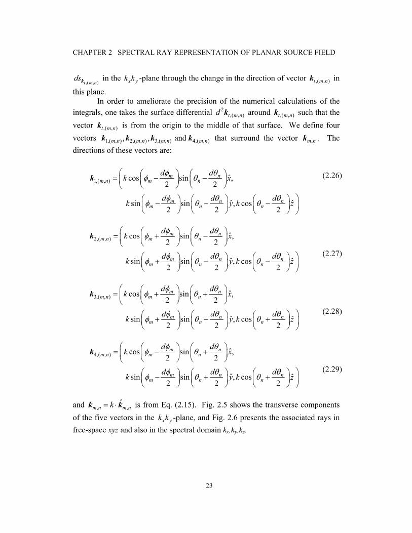
vector ,( , )t m nk is from the origin to the middle of that surface. We define four vectors 1,( , ) 2,( , ) 3,( , ) 4,( , ), , and m n m n m n m nk k k k that surround the vector ,m nk . The directions of these vectors are:
and , ,ˆ
m n m nk= ⋅k k is from Eq. (2.15). Fig. 2.5 shows the transverse components of the five vectors in the x yk k -plane, and Fig. 2.6 presents the associated rays in free-space xyz and also in the spectral domain kx,ky,kz.
1,( , ) ˆcos sin ,2 2
ˆ ˆ sin sin , cos2 2 2
m nm n m n
m n nm n n
d dk x
d d dk y k z
φ θφ θ
φ θ θφ θ θ
⎛ ⎛ ⎞ ⎛ ⎞= − −⎜ ⎜ ⎟ ⎜ ⎟⎝ ⎠ ⎝ ⎠⎝
⎞⎛ ⎞ ⎛ ⎞ ⎛ ⎞− − − ⎟⎜ ⎟ ⎜ ⎟ ⎜ ⎟⎝ ⎠ ⎝ ⎠ ⎝ ⎠ ⎠
k
(2.26)
2,( , ) ˆcos sin ,2 2
ˆ ˆ sin sin , cos2 2 2
m nm n m n
m n nm n n
d dk x
d d dk y k z
φ θφ θ
φ θ θφ θ θ
⎛ ⎛ ⎞ ⎛ ⎞= + −⎜ ⎜ ⎟ ⎜ ⎟⎝ ⎠ ⎝ ⎠⎝
⎞⎛ ⎞ ⎛ ⎞ ⎛ ⎞+ − − ⎟⎜ ⎟ ⎜ ⎟ ⎜ ⎟⎝ ⎠ ⎝ ⎠ ⎝ ⎠ ⎠
k (2.27)
3,( , ) ˆcos sin ,2 2
ˆ ˆ sin sin , cos2 2 2
m nm n m n
m n nm n n
d dk x
d d dk y k z
φ θφ θ
φ θ θφ θ θ
⎛ ⎛ ⎞ ⎛ ⎞= + +⎜ ⎜ ⎟ ⎜ ⎟⎝ ⎠ ⎝ ⎠⎝
⎞⎛ ⎞ ⎛ ⎞ ⎛ ⎞+ + + ⎟⎜ ⎟ ⎜ ⎟ ⎜ ⎟⎝ ⎠ ⎝ ⎠ ⎝ ⎠ ⎠
k (2.28)
4,( , ) ˆcos sin ,2 2
ˆ ˆ sin sin , cos2 2 2
m nm n m n
m n nm n n
d dk x
d d dk y k z
φ θφ θ
φ θ θφ θ θ
⎛ ⎛ ⎞ ⎛ ⎞= − +⎜ ⎜ ⎟ ⎜ ⎟⎝ ⎠ ⎝ ⎠⎝
⎞⎛ ⎞ ⎛ ⎞ ⎛ ⎞− + + ⎟⎜ ⎟ ⎜ ⎟ ⎜ ⎟⎝ ⎠ ⎝ ⎠ ⎝ ⎠ ⎠
k (2.29)

CHAPTER 2 SPECTRAL RAY REPRESENTATION OF PLANAR SOURCE FIELD
24
Figure 2.5: The transverse vector components 1,( , ) , m nk 2,( , ) ,m nk 3,( , )m nk
4,( , )and m nk and the surface differential 2,( , )t m nd k is covered by the
vectors in the x yk k -plane. The transverse component ,( , )t m nk is placed at
the center of 2,( , )t m nd k [62].
Given ( ), , ,( , ) ,( , )ˆ ˆ,t m n x m n y m nk x k y=k , the x, y, and z components of the electric field are found by
The equations (2.30) to (2.32) define a volume differential placed underneath the functions ( ) ( ) ( ), , , and ,x x y y x y z x yE k k E k k E k k , respectively, for the direction
( ) 2,( , ) ,( , ) ,( , )x m n x t m n t m nE E dΔ = ×k k (2.30)
( ) 2,( , ) ,( , ) ,( , )y m n y t m n t m nE E dΔ = ×k k (2.31)
( ) 2,( , ) ,( , ) ,( , )z m n z t m n t m nE E dΔ = ×k k (2.32)

CHAPTER 2 SPECTRAL RAY REPRESENTATION OF PLANAR SOURCE FIELD
25
,( , )t m nk . Fig. 2.2 shows the volume differential for the case of ( ),x x yE k k . Summing up the rays of the PWS as in Eq. (2.20), we find the total electric field at point P(x,y,z) is:
Given ( ),( , )x t m nE k and ( ),( , )y t m nE k , the component ( ),( , )z t m nE k is obtained using Eq. 2.6.
Figure 2.6: A ray of PWS arrives at point P(x,y,z) in the direction ,m nk in free-space xyz and in the spectral domain kxkykz [62].
The SRT enables the calculation of near-fields, and Eq. (2.33) consists of the sum total of the evanescent and non-evanescent rays of the PWS, which
( ) ( ) ( )( ),( , )
( , , )
,( , ) ,( , ) ,( , )
2,( , )
ˆ ˆ ˆ
ˆ ˆ ˆ
t m n
P x y z x y z
x t m n y t m n z t m nm n
jt m n
E x E y E z
E x E y E z
d e− ⋅
= + +
= + +
× ×
∑∑k r
E
k k k
k
(2.33)

CHAPTER 2 SPECTRAL RAY REPRESENTATION OF PLANAR SOURCE FIELD
26
propagate in +z direction and arrive at point P(x,y,z). The region 2 2x yk k k+ > in
the x yk k –plane correspond to the evanescent fields and their total effect is:
where
The ,nkρ and mφ are the polar coordinates of , ,m nρk in the x yk k –plane
with
and
The surface differential element is equal to
The PWS calculated using Eq. (2.1) and Eq. (2.2) are in the general complex variables and as a consequence, the x, y, and z field components transported by the rays of the PWS are complex. From Fig. 2.4 the vector
( , )m nΔE has Cartesian components ( , )x m nEΔ , ( , )y m nEΔ and ( , )z m nEΔ that contain the terms of the phase. The terms of phase have been added to the factor of time
j te ω to define the polarization of the rays of the PWS be it linearly, circularly or elliptically polarized.
( ) ( ) ( )2 2
, ,, ,
, , , , , ,1 1
2, ,
ˆ ˆ ˆ
m nm n
M
evanescent x m n y m n z m nn m
z kjm n
E x E y E z
d e e ρρ
ρ ρ ρ
ρ
+∞
= =
− −− ⋅
⎡ ⎤= + +⎣ ⎦
× × ×
∑∑
kk r
E k k k
k
(2.34)
, , , ,ˆ ˆ( cos( ) , sin( ) )m n n m n mk x k yρ ρ ρφ φ=k (2.35)
11 1 and
2 for 1
m mm m m M
d d
m M
φ φφ φ φ φ φ−−
+= + < <
< <
(2.36)
11 0; 2
2M
Md dφ φφ φ π +
= = − (2.37)
, 1 , ,1, , 1 ,1 with
2 2n n
n ndk dk dk
k k k kρ ρ ρρ ρ ρ
−−
+= + = + . (2.38)
2, , , ,m n n m nd k d dkρ ρ ρφ= × ×k . (2.39)

CHAPTER 2 SPECTRAL RAY REPRESENTATION OF PLANAR SOURCE FIELD
27
2.5 Discussion of Advantages and Disadvantages of SRT
In simulating the far-field and near-field of a structure, the SRT method has many advantages compared to other computational methods such as:
• The SRT can solve unbounded and open problems easily without
having to numerically model the space around scattering objects and radiating boundaries.
• The electric fields remain finite at caustic points.
• Effective in modeling electrically large structures with arbitrary 3D surfaces.
• The method can employ a simple ray tracing technique or be generalized to include the UAT and UTD diffraction theories.
• The SRT can model conductors and homogeneous dielectrics including reflection, refraction and diffraction.
• It saves the computer CPU time and memory.
• Since the media is linear, the solution and ray tubes obtained by the SRT for a particular structure can be interpreted as the transfer function of the structure. The transfer function of the structure can be re-used for the analysis of multi-antenna systems, for different frequencies, and optimization.
The shortcomings of the SRT, some of which are addressed in this research, are:
• To apply the SRT, the field distribution over the source plane containing the antenna should be known beforehand. It is difficult or impossible to obtain this knowledge from the SRT directly.
• Thorough ray tracing modules are needed to trace rays in complex structures.
• Not appropriate for modeling inhomogeneous media and the formulation in [60][62] does not model lossy media.
• Difficult to calculate input impedance and current distribution of an antenna with a complex structure, or a variation in the current distribution in the source plane due to the geometry of the complex structure.
CHAPTER 2 SPECTRAL RAY REPRESENTATION OF PLANAR SOURCE FIELD
28
• The SRT is not easily applicable to the resonance analysis as in [82]. However, in many practical cases, these resonances may not have any significant effect on radiated field.
• The size of the analyzed objects must be 4λ and up in terms of the wavelength.
• It cannot model complex multi-layer structures with sub-wavelength features, like an antenna, being close to large complex dielectric structures such as lens, and prisms.
2.6 Conclusions
In summary, in this chapter we have derived SRT solution using reciprocity theorem and Parseval’s theorem. The discretization of the PWS integrals in three dimensions was presented followed by discussion of the advantages and limits of SRT.
The hybridization of the SRT with rigorous numerical solvers such as the MoM, and the FEM to determine the field over the source plane is proposed in Chapter 3. If the field distribution on the source plane varies due to the geometry of the structure, then the SRT can find the new radiated field quickly. The antenna parameters such as the input impedance, directivity, and antenna efficiency can readily be calculated using a hybridization of the SRT.
29
CHAPTER 3
Proposed Hybrid Spectral Ray Tracing
Techniques
3.1 Introduction Hybrid techniques are reliable and accurate computational methods to
model multi-scale problems with complex discontinuities while exploiting the effectiveness of asymptotic methods. For problems where sub-wavelength features have to be modeled using rigorous methods, and complex structures with dimensions in the order of tens or even hundreds of wavelengths modeled by asymptotic methods, Spectral Ray Tracing (SRT) has a number of unique advantages. By including complex rays, SRT can effectively analyze both near-fields and far-fields accurately. Current-based methods such as PO are effective for the far-field analysis of electrically large and irregular shaped structures. However, the required current integrations are complex when compared to the proposed SRT using a matrix representation, which requires only one spectral integration per observation point regardless of the shape of the arbitrary 3D structure. The PO technique is also not as effective as SRT for near-field analysis.
SRT is based on the plane wave decomposition of the source field or a known current distribution [60]. The spectral samples of the plane waves are represented as ray tubes that leave the source plane and reach the observation point. The GTD, UTD or Uniform Asymptotic Theory (UAT)[35][37] are diffraction theories that are applied to these rays, where they undergo reflections, refractions, and diffractions. At the observation point, all the contributions from these rays are summed up to determine the total field.
In this chapter, a novel matrix representation of the SRT method, and Hybrid SRT (HSRT) methods based on a combination of MoM or FEM with SRT are proposed. For the first time, the SRT method is compared to the FEM computational technique employing commercial Ansoft HFSS[63]. Unlike the previous work [60]-[62] where it was only compared to PO, GO and
CHAPTER 3 PROPOSED HYBRID SPECTRAL RAY TRACING TECHNIQUES
30
measurements. The comparison uses the simulation of the terahertz Gaussian beam propagation through a hemispherical lens. We compared the computational time and accuracy of the SRT response with that of the HFSS through the convergence analysis.
A computationally efficient self-consistent Hybrid SRT method is proposed where the hybridization of FEM or MoM with SRT is a contribution to this research. The various versions of the HSRT method such as the FEM-SRT, and the MoM-SRT, are compared and validated with commercial software Ansoft HFSS for the FEM method, FEKO for the MoM, the Multi-level Fast Multipole Method (MLFMM) and PO via simulation of a bow-tie terahertz antenna backed by hyper-hemispherical silicon lens. It is shown that the MoM-SRT is more accurate than the MoM-PO and comparable in speed. The FEM-SRT method was able to accurately solve a double-slot antenna problem 77 times faster than the FEM exploiting the parallel processing. In addition, it is shown that the matrix formulation of SRT and HSRT is a promising approach for solving complex electrically large problems with high accuracy.
3.2 The Fast Analysis of Terahertz Integrated Lens Antennas
At terahertz frequencies, hyper-hemispherical silicon lens antennas are used to couple the terahertz radiation from the photoconductive antennas to free space. The lens and antenna have to be optimized for various applications such as in the terahertz radiation coupling from space to a Hot Electron Bolometer (HEB) [64]. In simulating the far-field and near-field radiation patterns of the lens antennas, the SRT method has many advantages compared to other computational methods. Like being easily adapted for optimization, and being able to solve unbounded and open problems easily. Unlike the FEM and FDTD methods, both are required numerically model the space around scattering objects and radiating boundaries.
3.2.1 SRT APPLICATION TO HYPER-HEMISPHERICAL LENS
In SRT, rays are introduced not as a result of the stationary phase condition [27],[31] or the stationary optical length with respect to small variations of the path, but rather as samples of the spectral plane waves. Suppose the source plane is the xy-plane at z = -d, then we calculate the 2D Fourier transform to get
( , )x x yE k k and ( , )y x yE k k

CHAPTER 3 PROPOSED HYBRID SPECTRAL RAY TRACING TECHNIQUES
31
An j te ω time dependence is assumed and the spectrum is discretized using rays along k , and θ φ . For the hyper-hemispherical lens, backward-ray launching is applied to determine the ray paths from the observation point O to the source plane. Due to reciprocity, this is the same path as from the source plane to the observation point. We then apply a different technique than in the past to determine the corresponding complex field amplitudes for each ray as we consider the pulse. In order to do backward-ray launching, we calculate
max , d and dφ φ θ→
as the function of the order of reflection (OR) [62][88]. Then set miniφ φ= and 1id dφ φ= .
Figure 3.1: The geometry of the hyper-hemispherical lens for tracing the
backward launched ray in the φ plane, courtesy of [62].
( )2
1( , ) ( , , )4
x yj k x k yx x y xE k k E x y d e dxdy
π+∞ +∞ +
−∞ −∞= −∫ ∫ (3.1)
( )2
1( , ) ( , , )4
x yj k x k yx x y yE k k E x y d e dxdy
π+∞ +∞ +
−∞ −∞= −∫ ∫ (3.2)
( , ) ( , )( , ) x x y x y x y y
z x yz
E k k k E k k kE k k
k+
= (3.3)
d

CHAPTER 3 PROPOSED HYBRID SPECTRAL RAY TRACING TECHNIQUES
32
Fig. 3.1 shows the hyper-hemispherical lens geometry in the φ plane. For a hyper-hemispherical lens, the minimum and maximum angles along θ are given by the parameters defined in Fig. 3.1:
where
'
min,1
cos( )arctan i ii
r rd R d
φθ
⎛ ⎞× −= ⎜ ⎟⎜ ⎟+ +⎝ ⎠
(3.4)
'
max, " "cos( )arcsin arcsin
i i
i ii
r rR Rφ φ
φθ
⎛ ⎞ ⎛ ⎞×⎜ ⎟ ⎜ ⎟= +⎜ ⎟ ⎜ ⎟⎝ ⎠ ⎝ ⎠
(3.5)
'
,1
cos( )arctan i isph i
r rd R
φθ
⎛ ⎞× −= ⎜ ⎟⎜ ⎟+⎝ ⎠
(3.6)
max, min,, 1 ,
,1,1i i
sph i sph iiNθ
θ θθ θ+
−= +
× (3.7)
1 , 1( ) tan( )sph iA d R θ += + × (3.8)
2 2
1 arccos2
r RA
iA
rφ
−
+
⎛ ⎞+⎜ ⎟=⎜ ⎟⎝ ⎠
(3.9)
1i i idφ φ φ+= − (3.10)
, min, 1, , ln ,
max, 1 min, 1
sph i ii cy i
i iN ceil Nθ θ
θ θθ θ
+
+ +
⎡ ⎤−= ⎢ ⎥
−⎢ ⎥⎣ ⎦ (3.11)
, min, 1ln,
, , ln
sph i icy i
i cyd
Nθ
θ θθ +−
= (3.12)
max, 1 , 1, , ,
max, 1 min, 1
i sph ii sph i
i iN ceil Nθ θ
θ θθ θ
+ +
+ +
⎡ ⎤−= ⎢ ⎥
−⎢ ⎥⎣ ⎦ (3.13)
max, 1 , 1,
, ,
i sph isph i
i sphd
Nθ
θ θθ + +−
= (3.14)
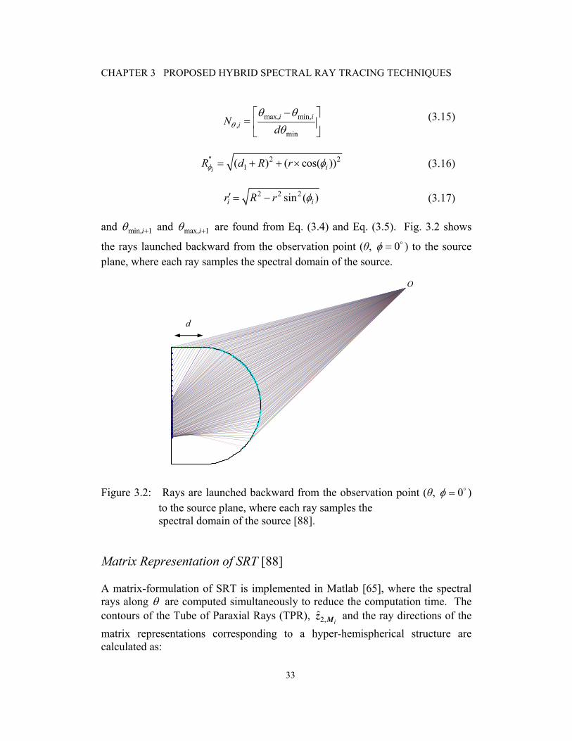
CHAPTER 3 PROPOSED HYBRID SPECTRAL RAY TRACING TECHNIQUES
33
and min, 1iθ + and max, 1iθ + are found from Eq. (3.4) and Eq. (3.5). Fig. 3.2 shows
the rays launched backward from the observation point (θ, 0φ = ) to the source plane, where each ray samples the spectral domain of the source.
Figure 3.2: Rays are launched backward from the observation point (θ, 0φ = ) to the source plane, where each ray samples the spectral domain of the source [88]. Matrix Representation of SRT [88] A matrix-formulation of SRT is implemented in Matlab [65], where the spectral rays along θ are computed simultaneously to reduce the computation time. The contours of the Tube of Paraxial Rays (TPR), 2,ˆ
iMz and the ray directions of the matrix representations corresponding to a hyper-hemispherical structure are calculated as:
max, min,,
min
i iiN
dθθ θ
θ−⎡ ⎤
= ⎢ ⎥⎣ ⎦
(3.15)
" 2 21( ) ( cos( ))
i iR d R rφ φ= + + × (3.16)
2 2 2sin ( )i ir R r φ′= − (3.17)
O
d

CHAPTER 3 PROPOSED HYBRID SPECTRAL RAY TRACING TECHNIQUES
34
where
and , 2iNi
θ ×∈ℜM
is a matrix, i is the index for ith φ component, i = 1,2,.., Nφ . For the rays hitting the spherical portion of the lens,
where
For the cylindrical part, the middle ray vector is given by
2, , ln , ln , ln , ln , ln , lnˆ ˆ ˆ ˆcos( )sin( ) sin( )sin( ) cos( )i i i i i icy cy cy cy cy cyx y z= +Mz +M M M M Mφ θ φ θ θ
(3.18)
, , ln
, ln
2
i
i cy
i i i
M cy
i i i N
d
dθ
φ φ φ
φ φ φ×
+⎡ ⎤⎢ ⎥= ⎢ ⎥⎢ ⎥+⎣ ⎦
φ (3.19)
, , ln
min, 1 min, 1
, ln
, , 2
i
i cy
i i
M cy
sph i sph i Nθ
θ θ
θ θ
+ +
×
⎡ ⎤⎢ ⎥= ⎢ ⎥⎢ ⎥⎣ ⎦
θ (3.20)
2, , , , , , ,ˆ ˆ ˆ ˆcos( )sin( ) sin( )sin( ) cos( )i i i i i isph sph sph sph sph sphx y z= +Mz +M M M M Mφ θ φ θ θ
(3.21)
, ,
,
2
i
i sph
i i i
M sph
i i i N
d
dθ
φ φ φ
φ φ φ×
+⎡ ⎤⎢ ⎥= ⎢ ⎥⎢ ⎥+⎣ ⎦
φ (3.22)
, ,
, 1 , 1
,
max, 1 max, 1 2
.i
i sph
sph i sph i
M sph
i i Nθ
θ θ
θ θ
+ +
+ + ×
⎡ ⎤⎢ ⎥
= ⎢ ⎥⎢ ⎥⎣ ⎦
θ (3.23)

CHAPTER 3 PROPOSED HYBRID SPECTRAL RAY TRACING TECHNIQUES
35
where
and , , ln 2, ln
i cyNi cy
θ ×∈ℜM is a matrix, i is the index for ith φ
component, i = 1,2,.., Nφ . minθ is the minimum angle that the ray is incident on the cylindrical section and sphθ is the minimum angle that strikes the spherical section of the hyper-hemispherical structure. For the spherical part, the middle ray vector is given by
where
2, , ln , , ln , , ln , , ln , , ln
, , ln
ˆ ˆ ˆcos( )sin( ) sin( )sin( )
ˆ cos( )i i i i i
i
m cy m cy m cy m cy m cy
m cy
x y
z
=
+Mz +M M M M
M
φ θ φ θ
θ
(3.24)
, , ln
12
, , ln12 ( 1) 1
i
i cy
i i
m cy
i i N
d
dθ
φ φ
φ φ− ×
⎡ ⎤+⎢ ⎥= ⎢ ⎥⎢ ⎥+⎣ ⎦
Mφ (3.25)
, , ln
1min, 1 ln,2
3min, 1 ln,2
, , ln3
, ln,21
, ln,2 ( 1) 1
i
i cy
i cy i
i cy i
m M cy
sph i cy i
sph i cy i N
d
d
d
dθ
θ θ
θ θ
θ θ
θ θ
+
+
− ×
⎡ ⎤+⎢ ⎥
+⎢ ⎥⎢ ⎥= ⎢ ⎥⎢ ⎥−⎢ ⎥
−⎢ ⎥⎣ ⎦
θ .
(3.26)
2, , , , , , , , , ,
, ,
ˆ ˆ ˆcos( )sin( ) sin( )sin( )
ˆ cos( )i i i i i
i
m sph m sph m sph m sph m sph
m sph
x y
z
=
+Mz +M M M M
M
φ θ φ θ
θ
(3.27)
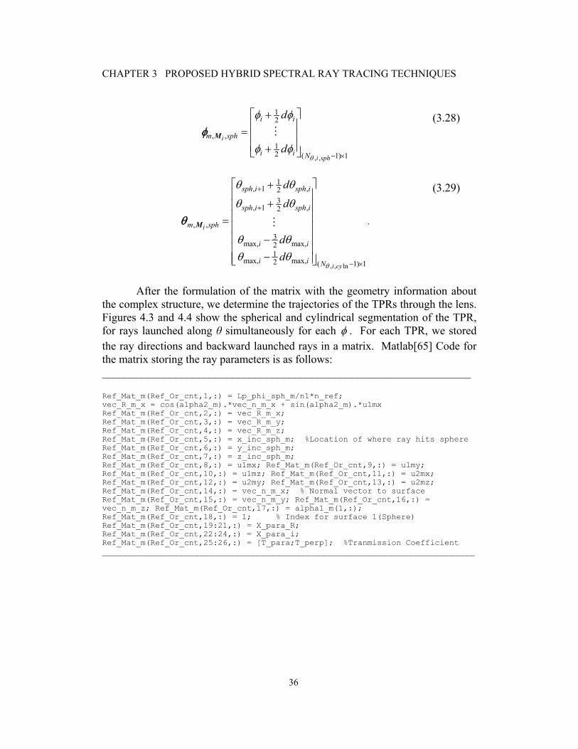
CHAPTER 3 PROPOSED HYBRID SPECTRAL RAY TRACING TECHNIQUES
36
After the formulation of the matrix with the geometry information about the complex structure, we determine the trajectories of the TPRs through the lens. Figures 4.3 and 4.4 show the spherical and cylindrical segmentation of the TPR, for rays launched along θ simultaneously for each φ . For each TPR, we stored the ray directions and backward launched rays in a matrix. Matlab[65] Code for the matrix storing the ray parameters is as follows: _________________________________________________________________
Ref_Mat_m(Ref_Or_cnt,1,:) = Lp_phi_sph_m/n1*n_ref; vec_R_m_x = cos(alpha2_m).*vec_n_m_x + sin(alpha2_m).*u1mx Ref_Mat_m(Ref_Or_cnt,2,:) = vec_R_m_x; Ref_Mat_m(Ref_Or_cnt,3,:) = vec_R_m_y; Ref_Mat_m(Ref_Or_cnt,4,:) = vec_R_m_z; Ref_Mat_m(Ref_Or_cnt,5,:) = x_inc_sph_m; %Location of where ray hits sphere Ref_Mat_m(Ref_Or_cnt,6,:) = y_inc_sph_m; Ref_Mat_m(Ref_Or_cnt,7,:) = z_inc_sph_m; Ref_Mat_m(Ref_Or_cnt,8,:) = u1mx; Ref_Mat_m(Ref_Or_cnt,9,:) = u1my; Ref_Mat_m(Ref_Or_cnt,10,:) = u1mz; Ref_Mat_m(Ref_Or_cnt,11,:) = u2mx; Ref_Mat_m(Ref_Or_cnt,12,:) = u2my; Ref_Mat_m(Ref_Or_cnt,13,:) = u2mz; Ref_Mat_m(Ref_Or_cnt,14,:) = vec_n_m_x; % Normal vector to surface Ref_Mat_m(Ref_Or_cnt,15,:) = vec_n_m_y; Ref_Mat_m(Ref_Or_cnt,16,:) = vec_n_m_z; Ref_Mat_m(Ref_Or_cnt,17,:) = alpha1_m(1,:); Ref_Mat_m(Ref_Or_cnt,18,:) = 1; % Index for surface 1(Sphere) Ref_Mat_m(Ref_Or_cnt,19:21,:) = X_para_R; Ref_Mat_m(Ref_Or_cnt,22:24,:) = X_para_i; Ref_Mat_m(Ref_Or_cnt,25:26,:) = [T_para;T_perp]; %Tranmission Coefficient _________________________________________________________________________
, ,
12
, ,12 ( 1) 1
i
i sph
i i
m sph
i i N
d
dθ
φ φ
φ φ− ×
⎡ ⎤+⎢ ⎥= ⎢ ⎥⎢ ⎥+⎣ ⎦
Mφ (3.28)
, , ln
1, 1 ,2
3, 1 ,2
, ,3
max, max,21
max, max,2 ( 1) 1
i
i cy
sph i sph i
sph i sph i
m sph
i i
i i N
d
d
dd
θ
θ θ
θ θ
θ θθ θ
+
+
− ×
⎡ ⎤+⎢ ⎥
+⎢ ⎥⎢ ⎥=⎢ ⎥⎢ ⎥−⎢ ⎥
−⎢ ⎥⎣ ⎦
Mθ .
(3.29)
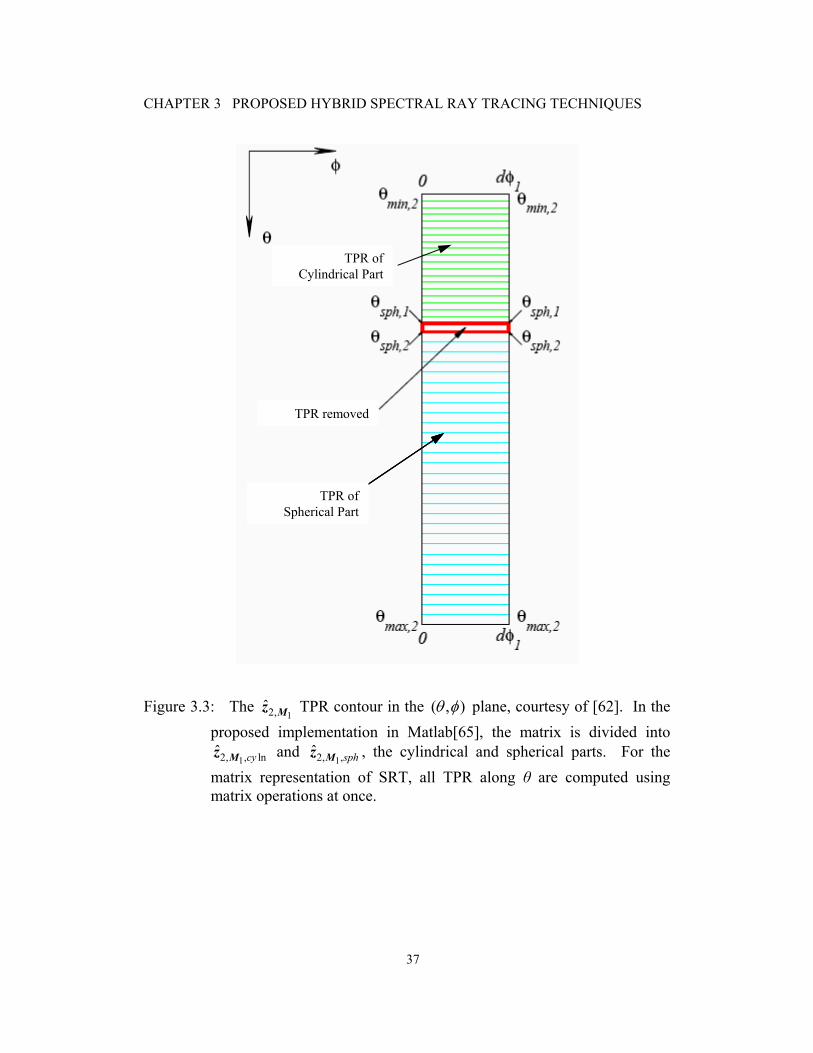
CHAPTER 3 PROPOSED HYBRID SPECTRAL RAY TRACING TECHNIQUES
37
Figure 3.3: The 12,ˆ Mz TPR contour in the ( , )θ φ plane, courtesy of [62]. In the
proposed implementation in Matlab[65], the matrix is divided into
12, , lnˆ cyMz and 12, ,ˆ sphMz , the cylindrical and spherical parts. For the
matrix representation of SRT, all TPR along θ are computed using matrix operations at once.
TPR removed
TPR of Spherical Part
TPR of Spherical Part
TPR of Spherical Part
TPR of Cylindrical Part

CHAPTER 3 PROPOSED HYBRID SPECTRAL RAY TRACING TECHNIQUES
38
Figure 3.4: The matrix 2,ˆiMz TPR in the ( , )θ φ plane [62] and the 2,ˆ
im Mz vector, which is the middle ray of the matrix.
Summing up all the ray contributions we find the total electric field at point O(x, y, z):
where
(
) ,( , )
( , , )
,( , ) ,( , )
2,( , ) ,( , )
ˆ ˆ ˆ
ˆ ˆ ( ) ( )
ˆ ( ) t m n
O x y z x y z
x t m n y t m nm n
jz t m n t m n
E E E
E E
E d e− ⋅
= + +
= +
+ ⋅ ⋅
∑∑k r
E x y z
k x k y
k z k
(3.30)
2
2,( , ) sin(2 )
2t m n n n mkd d dθ θ φ=k . (3.31)
2,ˆim Mz

CHAPTER 3 PROPOSED HYBRID SPECTRAL RAY TRACING TECHNIQUES
39
3.2.2 Algorithm to Calculate the Integral of the Spectrum [88]
Step 1 Enter parameters of the lens, point of observation P and order of
reflection OR.
Step 2 Calculate max , d and dφ φ θ→
as function of OR.
Step 3 Set i = 0, 0totalE = , miniφ φ= and 1id dφ φ= .
Step 4 Calculate the next iterate 2,ˆiMz and ,2, imz M .
Step 5 Determine the trajectories of the TPRs through the lens. Step 6 If these TPRs depart the z=-d plane go to Step 7. Step 7 Calculate ,2,( )
jmE z M , field created by the TPRs, and
,2, ,2, ,2,( ) ( ) ( )i i jm m mE z E z E z= +M M M .
Step 8 Calculate ,2,( )
itotal total mE E E z= + M . Step 9 Find 1i i idφ φ φ+ = + , Set i = i+1. Step 10 If maxiφ φ> then store totalE , else go to Step 4. The algorithm is implemented in Matlab[65].
3.2.3 Comparison of the FEM with the SRT [88]
The SRT method is compared with the FEM by the simulation of the terahertz Gaussian beam propagation through a hemispherical lens. The Terahertz Gaussian beam propagation through a silica ( 3.8rε = ) dielectric hemispherical lens is simulated using the SRT and the FEM. In order to simulate the lens using the FEM in Ansoft HFSS[63], the radius of the hemispherical lens is set to R = 5 mm. The lens bottom at z =0 mm is a Perfect Electric Conductor (PEC). Fig. 3.5 shows the geometry of this lens.

CHAPTER 3 PROPOSED HYBRID SPECTRAL RAY TRACING TECHNIQUES
40
Figure 3.5: The geometry of the 5 mm radius (7.3λ) hemispherical lens.
A Gaussian beam is incident on the z = 0 mm plane and polarized along
the x direction
where 0 1 V/mE = , the beam waist of 0 2 mmw = and ( , ) 0yE x y = . The focal point is (0, 0, 0 mm). The operating frequency is 112.5 GHz. The corresponding spectral distribution is given by:
Fig. 3.6 shows the simulation results for a far-field E-plane radiation pattern of the hemispherical lens antenna with a Gaussian source using: i) a Geometrical Optics (GO) approximation, ii) the SRT method with no multiple reflections and iii) the Ansoft HFSS[63]. Fig. 3.7 shows the SRT and GO solutions for a mm hyper-hemispherical silica lens (d = 12.84 mm) with R = 25. The SRT algorithm is implemented in Matlab [65]. The observation points used were 0 90θ≤ ≤ . The GO is simulated using spherical waves that originated
2 2
20
0( , )x y
wxE x y E e
⎛ ⎞+⎜ ⎟−⎜ ⎟⎝ ⎠=
(3.32)
2 2 20
2 2 20
( )20 0 4
( )20 0 4
2 2 2
( , ) , ( , ) 04
( , )( , ) .
4
x y
x y
w k k
x x y y x y
w k kx x y x x
z x yz x y
E wE k k e E k k
E k k k k E wE k k ek k k k
π
π
+−
+−
= =
⋅= − = −
− −
(3.33)

CHAPTER 3 PROPOSED HYBRID SPECTRAL RAY TRACING TECHNIQUES
41
from the center of the source plane, which are refracted at the lens surface and arrived to the observation point. The wavefront of the refracted rays are calculated using a divergence factor and the curvature matrix of a spherical surface. The HFSS FEM simulation took 1 hour, 48 minutes and 12 seconds on a PC with the Intel Centrino Duo 2.4 GHz processor and 4 GB of RAM. The SRT took 3 minutes and 52 seconds on the same PC to obtain the result in Fig. 3.6. The L2 norm difference between the SRT and HFSS responses is 2SRT FEM−R R is 0.1312. Convergence analysis shows that increasing the ray density from 72,000 to 1 million, results in a reduction from 10-5 to 2 ×10⁻⁷ in the norm of the difference between Ex response of successive iterations. Thus SRT is computationally fast compared to the FEM method for solving quasi-optical EM problems.
Rad
iatio
n P
atte
rn in
dB
Phas
e in
Deg
rees
30 -20
-15
-10
-5
0
0 15 25-180
-90
0
90
180
5 10 20 (degrees)θ
Figure 3.6: The E-plane far-field, Ex radiation pattern in dB and phase of
electric field obtained using SRT for the R = 5 mm hemispherical lens with 3.8rε = [88].
SRT (--) GO ( · ) HFSS (-o-)

CHAPTER 3 PROPOSED HYBRID SPECTRAL RAY TRACING TECHNIQUES
42
-30 -25 -20 -15 -10 -5 0 5 10 15 20 25 30-40
-35
-30
-25
-20
-15
-10
-5
0R
adia
tion
Patte
rn in
dB
-270
-180
-90
0
90
180
270
Pha
se in
Deg
rees
θ (degrees) Figure 3.7: The E-plane far-field, Ex radiation pattern in dB and phase of
electric field obtained using SRT and GO for the R = 25 mm hyper-hemispherical silica lens (d = 12.84 mm)[88].
In backward launching rays, the density of the rays along the θ direction
is determined by bwrldNθ
πθ = , where Nθ is varied for 12 iteration indices. The
values of Nφ and Nθ for the case of convergence analysis of increasing ray density along θ are shown in Table 3.1.
TABLE 3.1: Iteration index vs. ray density
i 1 2 3 4 5 6 7 8 9 10 Nθ 36 72 144 260 360 560 760 860 1360 1860
Let ( )i
θR be the magnitude of the far-field electric field along the x-direction (Ex) at the current iterate i with a specified number of rays launched
SRT (--) GO ( -×- )
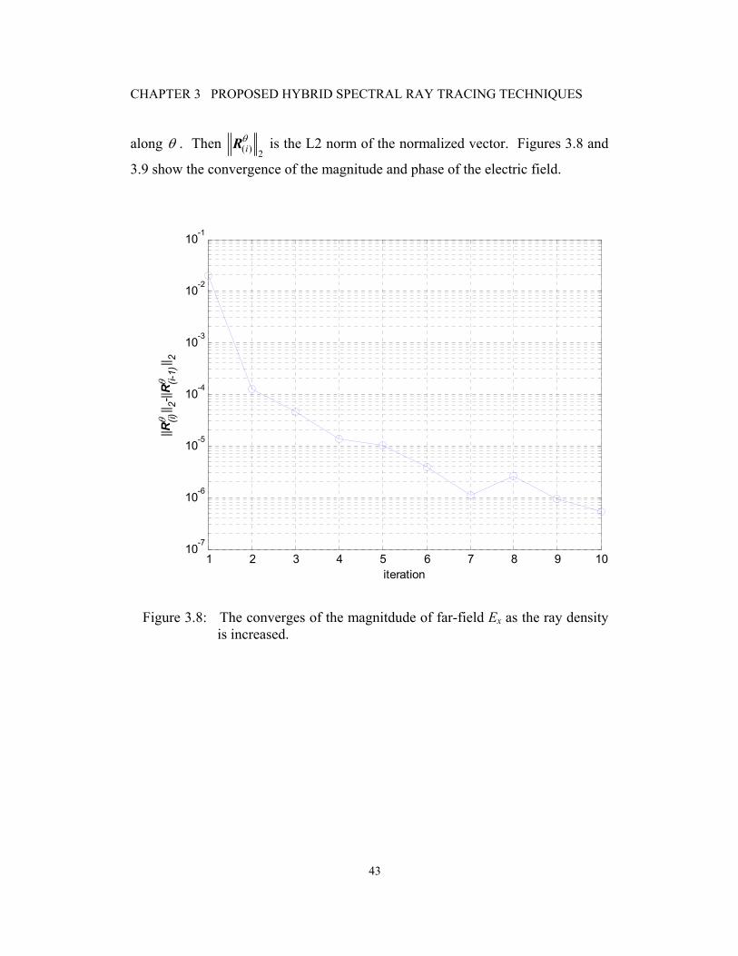
CHAPTER 3 PROPOSED HYBRID SPECTRAL RAY TRACING TECHNIQUES
43
along θ . Then ( ) 2iθR is the L2 norm of the normalized vector. Figures 3.8 and
3.9 show the convergence of the magnitude and phase of the electric field.
1 2 3 4 5 6 7 8 9 1010-7
10-6
10-5
10-4
10-3
10-2
10-1
iteration
||R(i)θ
|| 2-||R (i-
1)θ
|| 2
Figure 3.8: The converges of the magnitdude of far-field Ex as the ray density
is increased.
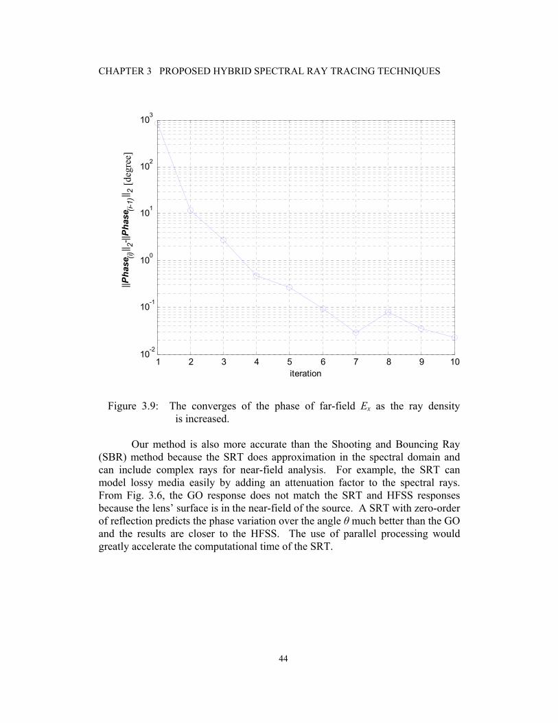
CHAPTER 3 PROPOSED HYBRID SPECTRAL RAY TRACING TECHNIQUES
44
1 2 3 4 5 6 7 8 9 1010-2
10-1
100
101
102
103
iteration
||Pha
se(i)
|| 2-||Ph
ase (i-
1)|| 2
Figure 3.9: The converges of the phase of far-field Ex as the ray density
is increased. Our method is also more accurate than the Shooting and Bouncing Ray
(SBR) method because the SRT does approximation in the spectral domain and can include complex rays for near-field analysis. For example, the SRT can model lossy media easily by adding an attenuation factor to the spectral rays. From Fig. 3.6, the GO response does not match the SRT and HFSS responses because the lens’ surface is in the near-field of the source. A SRT with zero-order of reflection predicts the phase variation over the angle θ much better than the GO and the results are closer to the HFSS. The use of parallel processing would greatly accelerate the computational time of the SRT.
[deg
ree]

CHAPTER 3 PROPOSED HYBRID SPECTRAL RAY TRACING TECHNIQUES
45
3.3 HYBRIDIZATION OF SPECTRAL RAY TRACING
In the proposed rigorous Hybrid SRT (HSRT) method, the spectral ray method is combined with a rigorous numerical solver to model complex multi-layer structures with sub-wavelength features or an antenna close to large complex dielectric structures such as lens, and prisms. The proposed Hybrid SRT (HSRT) method is simple to implement and can also deal with the diffraction of an arbitrary wave, where the incident wave is decomposed into plane waves.
The hybridization of spectral ray tracing with the Finite Element Method (FEM) and the Method of Moments (MoM) is essential because to apply the SRT, the field distribution or current distribution over the source plane containing the antenna should be known beforehand. Usually, an analytical expression for the field distribution in the source plane might not be a problem. In addition, a typical quasi-optical system may contain structures that cannot be analyzed using the SRT such as multi-layer structures with sub-wavelength features, or a planar antenna close to large complex dielectric structures such as lens and prisms. Special material such as left handed material or anisotropic material cannot be handled accurately using the SRT, because the SRT assumes the structure’s material is homogenous and isotropic. The general HSRT method then uses the MoM, the FEM, or the FDTD to determine the field over the source plane. The structures with complex discontinuities and/or sub-wavelength features are isolated from the rest of the problem in a virtual box. The scattering and diffraction effects are simulated using rigorous numerical solvers. The amplitude and phase of the fields obtained using commercial FEM and/or MoM solvers in the virtual box are connected to the rest of the problem by applying boundary conditions. Then the SRT uses these field solutions as a starting point for the plane wave decomposition, where the SRT is applied for the rest of the complex electrically large structure. Fig. 3.10 shows the structures analyzed using FEM and/or MoM surrounded by virtual boxes for an integrated lens antenna example.
The reasons that the SRT method is advantageous in the hybridization with the rigorous numerical methods are as follows:
1) The SRT can calculate near-field and far-field without any approximations and includes the complex rays for accurate analysis of the complex electrically large structures over a wide range of frequencies. The GO and the PO on the other hand are effective for far-field calculations at high frequencies.
2) The SRT is based on the Spectral Theory of Diffraction (STD)[31] and so it can deal with the diffraction of an arbitrary wave, where the incident wave is decomposed into plane waves.

CHAPTER 3 PROPOSED HYBRID SPECTRAL RAY TRACING TECHNIQUES
46
3) The SRT has the advantage compared to the FEM and the FDTD in being able to solve unbounded and open problems easily without having to numerically model the space around scattering objects and radiating boundaries.
4) Since the SRT is based on ray tracing techniques, it can exploit the mature area of ray tracing, such as Non Uniform Rational Basis Spline (NURBS) surfaces and Monte Carlo ray tracing methods to effectively model arbitrary 3D structures.
3.3.1 Hybrid Spectral Ray Tracing (HSRT)[96]
The HSRT technique has in general the following stages. The first stage is to determine the source near-field using a numerical rigorous method like the FEM or the MoM. In the second stage the SRT method is applied. Then in the third stage, we correct (or update) the near-field distribution of the source using the rays coming back towards the source and thus repeat stages 2, 3 until it the solution converges.
Figure 3.10 is used to describe the method in more detail through its application to a particular example of radiation from a planar antenna attached to a lens. First, the near-field of a planar antenna such as a bow-tie antenna will be obtained using a rigorous method applied to a simplified configuration consisting of the antenna element and its immediate surroundings (the region bounded by dotted line in Fig. 3.10). Then the SRT will be applied to the aforementioned near-field to find fields everywhere.
Figure 3.10: The Integrated lens antenna with structures that are analyzed
by rigorous numerical methods surrounded by virtual boxes.
CHAPTER 3 PROPOSED HYBRID SPECTRAL RAY TRACING TECHNIQUES
47
Stage 1: In this step, the planar antenna is replaced with equivalent
surface currents ˆS n= ×J H and ˆS n= ×M E
induced by an impressed electromagnetic field [29] at the interior boundary between the source and the complex electrically large multi-layer dielectric.
The Electric-Field Integral Equation (EFIE) is employed to find the tangential field over the boundary between the source plane and the large dielectric. In this initial step the lens is replaced by an infinite dielectric half space. The EFIE is
Where 'R = -r r is the distance between any source element and observation point S∈r . The EFIE Eq. (3.34) is solved for an unknown source current J over z = -d plane in terms of the known primary (impressed) source field tan
iE . A commercial numerical solver like the FEKO MoM [73] or the HFSS FEM [63] can be used at this initial stage (See Fig. 3.11).
The EFIE Eq. (3.34) is used in an iterative procedure to find the accurate source current and the radiated field. The initial incident field is the impressed source field tan,0
iE , which will be used as the known excitation in Eq. (3.34). EFIE is then solved for the unknown source current J
using any existing commercial solver.
Stage 2: The SRT will be applied to J
to find the fields everywhere including those reflected or scattered back towards the source. The latter fields will be added to the initial surface source field over z = -d to produce an updated planar source field.
Stage 3: The updated source field will be used. These Neumann iterative steps will be repeated until desired precision defined by
( 1) ( )tan tan
( )tan
j j
j
+ −E E
E is achieved.
The whole iterative solution process is described in Fig. 3.12. The iterative technique is similar to [46] but the initial approximation for the incident near-field or current distribution over the boundary of the electrically large region is obtained using a full-wave simulator. The effect of the reflected spectral rays is included by adding the contributions to the spectral component of the source field.
Going back to the example illustrated in Fig. 3.10, first, the initial source field due to the near-field radiation from the planar antenna is found by solving
2
'tan
( ') ( ( ')) ( )4
SS
jkRi
j k j
e dSR
ωεπωε
−
⎡ ⎤+ − ×⎣ ⎦
× = −
∫ ∫ r r MiJ J
E
∇ ∇ ∇
(3.34)

CHAPTER 3 PROPOSED HYBRID SPECTRAL RAY TRACING TECHNIQUES
48
the EFIE using a MoM solver or a FEM solver in a lossless dielectric half-space (See Fig. 3.11).
12.9rε =
11.9rε =
0.15 mm
Figure 3.11: The planar layered structure used to find the initial near-
field distribution of the THz or the millimeter-wave planar antenna that radiates to an electrically large dielectric (refer to area surrounded by dotted line in Fig. 3.10 ). The substrate is LTG-GaAs and the dielectric half-space is silicon ( 11.9rε = ).
The near-field over the z = -d plane becomes the initial near-field
distribution used as a boundary field distribution to solve the electrically-large dielectric structure using the SRT. The tangential field must be continuous across the boundary between the Low-Temperature-Grown (LTG)-GaAs substrate with a height of 150 μm (region 1) and an electrically-large hyper-hemispherical silicon lens (region 2). The boundary condition is:
Which has already been included in the numerical (MoM or FEM) solution of the planar antenna. In the next step, the boundary fields expressed in Eq. (3.35) are used to find the PWS of the source. The z-component of the electric field over the source plane is not used in the spectral ray extraction process. Instead, the z-component of the spectrum is computed using Eq. (3.3). Then the Fourier transform is calculated as:
(1) (2)
(1) (2)
( , , ) ( , , )
( , , ) ( , , )x x
y y
E x y d E x y d
E x y d E x y d
− = −
− = − (3.35)
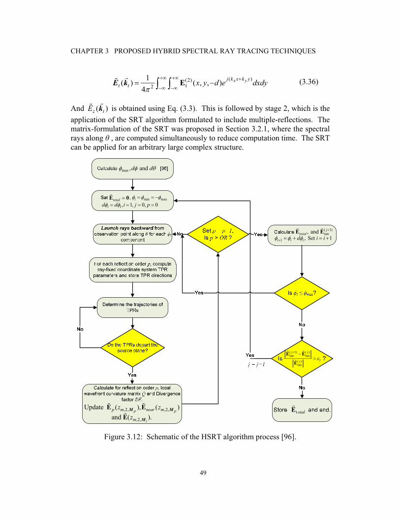
CHAPTER 3 PROPOSED HYBRID SPECTRAL RAY TRACING TECHNIQUES
49
And ( )z tE k is obtained using Eq. (3.3). This is followed by stage 2, which is the application of the SRT algorithm formulated to include multiple-reflections. The matrix-formulation of the SRT was proposed in Section 3.2.1, where the spectral rays along θ , are computed simultaneously to reduce computation time. The SRT can be applied for an arbitrary large complex structure.
total =E 0 min maxiφ φ φ= = −
1, 1, 0, 0id d i j pφ φ= = = =
t otalE
( 1)tan, and j
total+E E
1 , Set 1i i id i iφ φ φ+ = + = +
( 1) ( )tan tan
1( )tan
j j
jε
+ −>
E E
E
,2, ,2,Update ( ), ( )p pp m near mz z E EM M
,2,and ( ).imz ME
max , and d dφ φ θ
Figure 3.12: Schematic of the HSRT algorithm process [96].
( )(2)
t21( ) ( , , )
4x yj k x k y
t t x y d e dxdyπ
+∞ +∞ +
−∞ −∞= −∫ ∫ EE k (3.36)

CHAPTER 3 PROPOSED HYBRID SPECTRAL RAY TRACING TECHNIQUES
50
3.3.2 HSRT Algorithm to Calculate Integral of the Spectrum [96] In this section the HSRT algorithm is presented in detail.
Step 1 Define the source and antenna structure in a dielectric half-space with the dielectric constant of the lens or other structure that is in proximity to the antenna. Enter the geometry parameters of the electrically large structure, the point of observation P and the order of reflection OR.
Step 2 Simulate the structure using MoM or FEM.
Step 3 Extract the spectral rays by calculating the spectrum of the Electric field over the source plane. Extract the spectral rays by calculating PWS of the source (0)
tanE using GPU.
Step 4 Calculate max ,d and dφ φ θ→
as function of OR.
Step 5 Set i = 1, j = 0, p = 0, 0total =E , miniφ φ= and 1id dφ φ= .
Step 6 Launch rays backward from observation point along θ for each ϕi component. Calculate the next iterate 2, ,ˆ
i sphMz , 2, , lnˆi cyMz and
corresponding middle ray directions ,2,ˆim Mz .
Step 7 Determine the trajectories of the TPRs through the electrically-large complex dielectric structure.
Step 8 If these TPRs depart the z=-d plane go to Step 9 else go to Step 7. Step 9 Calculate ,2,( )
pmzE M , the field created by the TPRs, and
,2, ,2, ,2,( ) ( ) ( )i i pm m mz z z= +E E EM M M . The spectrum of the near-
field obtained using the MoM or FEM method in the source plane is employed to calculate ,2,( )
pnear mzE M .
Step 10 Set p = p+1. If p > OR, calculate ,2,( )itotal total mz= +E E E M , and
update near-field ( 1) ( )tan tan ,2,( )
p
j jnear mz+ = +E E E M else go to Step 6.
Step 11 Find 1i i idφ φ φ+ = + , Set i = i+1.

CHAPTER 3 PROPOSED HYBRID SPECTRAL RAY TRACING TECHNIQUES
51
Step 12 If maxiφ φ≤ , go to Step 6.
Step 13 If ( 1) ( )tan tan
1( )tan
j j
jε
+ −>
E E
E , continue j = j+1 and go to Step 5, else store
totalE .
The Neumann iteration process continues until user-defined convergence parameter is met, and i denotes an appropriate vector norm.
3.4 Applications of the Hybrid Method
3.4.1 THz integrated Bow-Tie Antenna [90][96]
A bow-tie antenna backed by a silicon ( 11.9rε = ) dielectric hyper-hemispherical lens is used to simulate the THz transmitter-receiver link in free-space. The advantages of the bow-tie antenna are its simple design and broad-band impedance. The planar bow-tie antenna covers a surface area of 3.466 mm × 2 mm and is placed on a 150 μm thick LTG-GaAs ( 12.9rε = ) substrate. In the setup, an edge-coupled or vertically-coupled traveling-wave photomixer integrated with a CoPlanar Stripline (CPS) [66] is simulated at the operating frequency of 100 GHz. The opening angle of the bow-tie is 60o. The CPS line has a strip width of 20 μm and a gap of 10 μm. The substrate is then backed by a 10 mm diameter hyper-hemispherical Si lens with a 0.84 mm cylindrical extension as shown in Fig. 3.10. Fig. 3.13 shows the geometry of the planar bow-tie antenna and coordinate system used in this thesis. The x-axis points along the axis of the dipole and the z-axis is the optical axis.
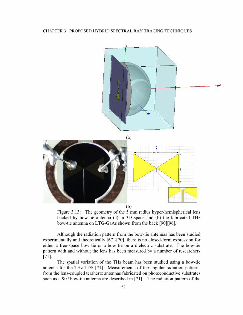
CHAPTER 3 PROPOSED HYBRID SPECTRAL RAY TRACING TECHNIQUES
52
(a)
(b)
Figure 3.13: The geometry of the 5 mm radius hyper-hemispherical lens backed by bow-tie antenna (a) in 3D space and (b) the fabricated THz bow-tie antenna on LTG-GaAs shown from the back [90][96].
Although the radiation pattern from the bow-tie antennas has been studied
experimentally and theoretically [67]-[70], there is no closed-form expression for either a free-space bow tie or a bow tie on a dielectric substrate. The bow-tie pattern with and without the lens has been measured by a number of researchers [71].
The spatial variation of the THz beam has been studied using a bow-tie antenna for the THz-TDS [71]. Measurements of the angular radiation patterns from the lens-coupled terahertz antennas fabricated on photoconductive substrates such as a 90ᴼ bow-tie antenna are described in [71]. The radiation pattern of the

CHAPTER 3 PROPOSED HYBRID SPECTRAL RAY TRACING TECHNIQUES
53
free-space antenna is modified by the presence of a high-dielectric substrate. As with the dipole antennas, most of the radiated energy from a bow-tie antenna on a high dielectric substrate is directed into the substrate [67].
In [71], the radiated field using a dipole radiation pattern is employed instead of a finite-element analysis of the bow-tie. Noting that the bow-tie is not dramatically dissimilar to that of a conventional dipole pattern [67]. Here the authors run a FEM and MoM simulation to find the near-field radiation pattern of the bow-tie antenna. The small refractive index discontinuity at the interface of the GaAs substrate and silicon lens is neglected and the entire structure is assigned the refractive index of silicon. Once the field on the inner surface of the substrate lens is found, the external field is calculated by accounting for the refraction through the surface without considering the multiple-reflections and diffraction through the finite exit aperture of the substrate lens. The diffraction through the finite aperture due to the lens is described by a Fresnel-Kirchoff diffraction calculation [72]. In [71], the vector nature of the field is neglected, so no information about the polarization of the diffracted wave can be obtained.
The proposed HSRT approach, the FEM-SRT and the MoM-SRT techniques, model the THz propagation through free-space including polarization information.
The Application of HSRT: The FEM-SRT Technique [90] The planar bow-tie antenna including the CPS line in the dielectric half-
space is modeled using the FEM in Ansoft HFSS[63] to find the near-field distribution in the aperture plane z = -d. Considering the lens and substrate as a planar layered medium which is transversely unbounded with respect to the z axis, it is possible to utilize 2-D Fourier transform to convert any field component in the spatial domain to its corresponding component in the spectral domain. The planar layered structure used for finding the near-field of the bow-tie antenna on the LT-GaAs substrate and backed by silicon lens is shown in Fig. 3.10. The TEM mode of the CPS is excited at the operating frequency of 100 GHz. Although the CPS line can be excited in HFSS, another proposed model excites the antenna using a lumped voltage source across the gap with a width of
10g mμ λ= . This is beneficial since the CPS TEM mode electric field is produced by a nonlinear photocurrent impressed on the LTG-GaAs slab and free-space interface. This can be used in an optimization procedure to determine the radiated field and power due to the photocurrent. The solution procedure proceeds from the assumption that a THz wave is exciting a CPS line.
The simulation time to find the near-field was 26 minutes and 2 seconds requiring 4.34 GB of RAM on a PC with an Intel Centrino Duo 2.4 GHz processor and 6 GB of RAM. Once the near-field distribution in the plane z = -d is found, 2-D Fourier transform finds the field in the spectral domain. Fig. 3.14
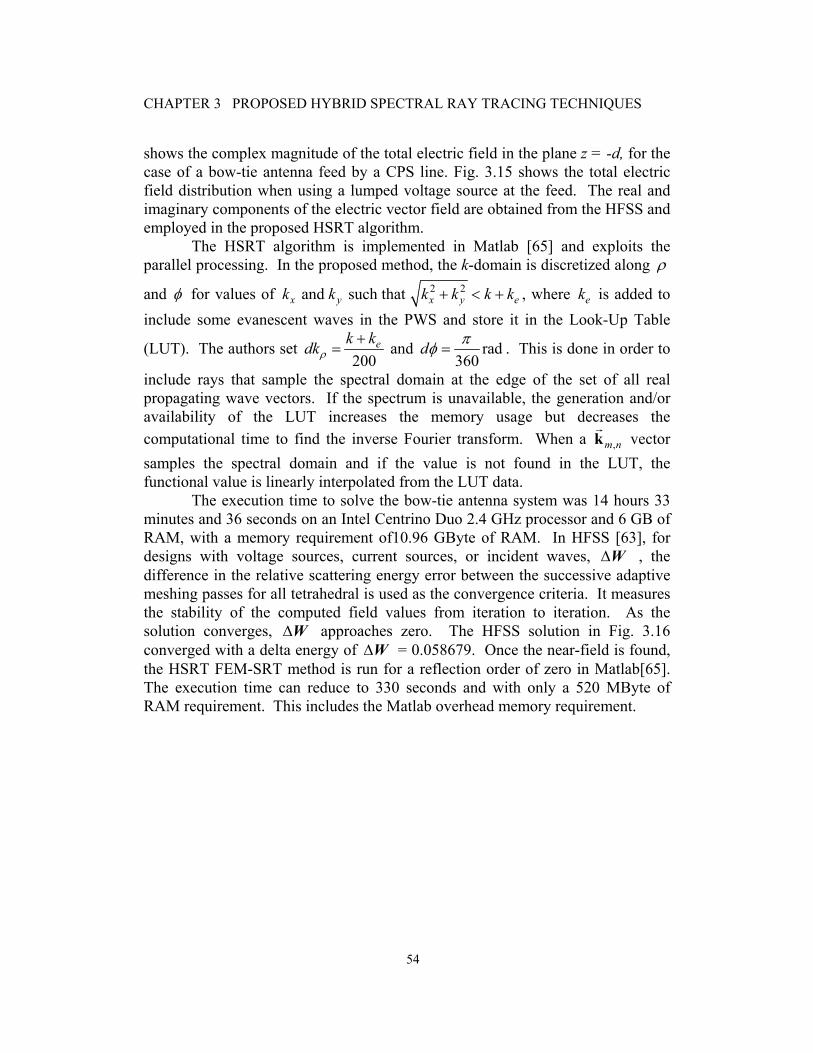
CHAPTER 3 PROPOSED HYBRID SPECTRAL RAY TRACING TECHNIQUES
54
shows the complex magnitude of the total electric field in the plane z = -d, for the case of a bow-tie antenna feed by a CPS line. Fig. 3.15 shows the total electric field distribution when using a lumped voltage source at the feed. The real and imaginary components of the electric vector field are obtained from the HFSS and employed in the proposed HSRT algorithm.
The HSRT algorithm is implemented in Matlab [65] and exploits the parallel processing. In the proposed method, the k-domain is discretized along ρ
and φ for values of 2 2 and such that x y x y ek k k k k k+ < + , where ek is added to include some evanescent waves in the PWS and store it in the Look-Up Table
(LUT). The authors set 200
ek kdkρ+
= and rad360
d πφ = . This is done in order to
include rays that sample the spectral domain at the edge of the set of all real propagating wave vectors. If the spectrum is unavailable, the generation and/or availability of the LUT increases the memory usage but decreases the computational time to find the inverse Fourier transform. When a ,m nk vector samples the spectral domain and if the value is not found in the LUT, the functional value is linearly interpolated from the LUT data.
The execution time to solve the bow-tie antenna system was 14 hours 33 minutes and 36 seconds on an Intel Centrino Duo 2.4 GHz processor and 6 GB of RAM, with a memory requirement of10.96 GByte of RAM. In HFSS [63], for designs with voltage sources, current sources, or incident waves, ΔW , the difference in the relative scattering energy error between the successive adaptive meshing passes for all tetrahedral is used as the convergence criteria. It measures the stability of the computed field values from iteration to iteration. As the solution converges, ΔW approaches zero. The HFSS solution in Fig. 3.16 converged with a delta energy of ΔW = 0.058679. Once the near-field is found, the HSRT FEM-SRT method is run for a reflection order of zero in Matlab[65]. The execution time can reduce to 330 seconds and with only a 520 MByte of RAM requirement. This includes the Matlab overhead memory requirement.
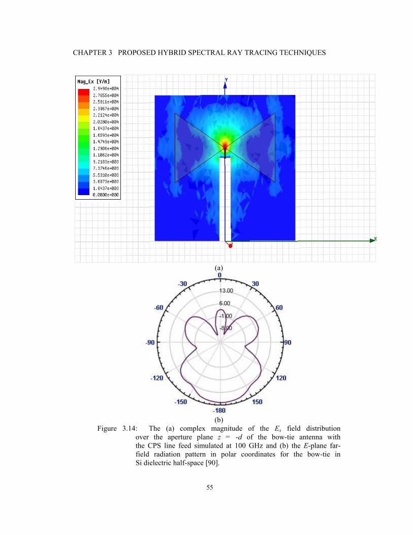
CHAPTER 3 PROPOSED HYBRID SPECTRAL RAY TRACING TECHNIQUES
55
(a)
(b)
Figure 3.14: The (a) complex magnitude of the Ex field distribution over the aperture plane z = -d of the bow-tie antenna with the CPS line feed simulated at 100 GHz and (b) the E-plane far- field radiation pattern in polar coordinates for the bow-tie in Si dielectric half-space [90].
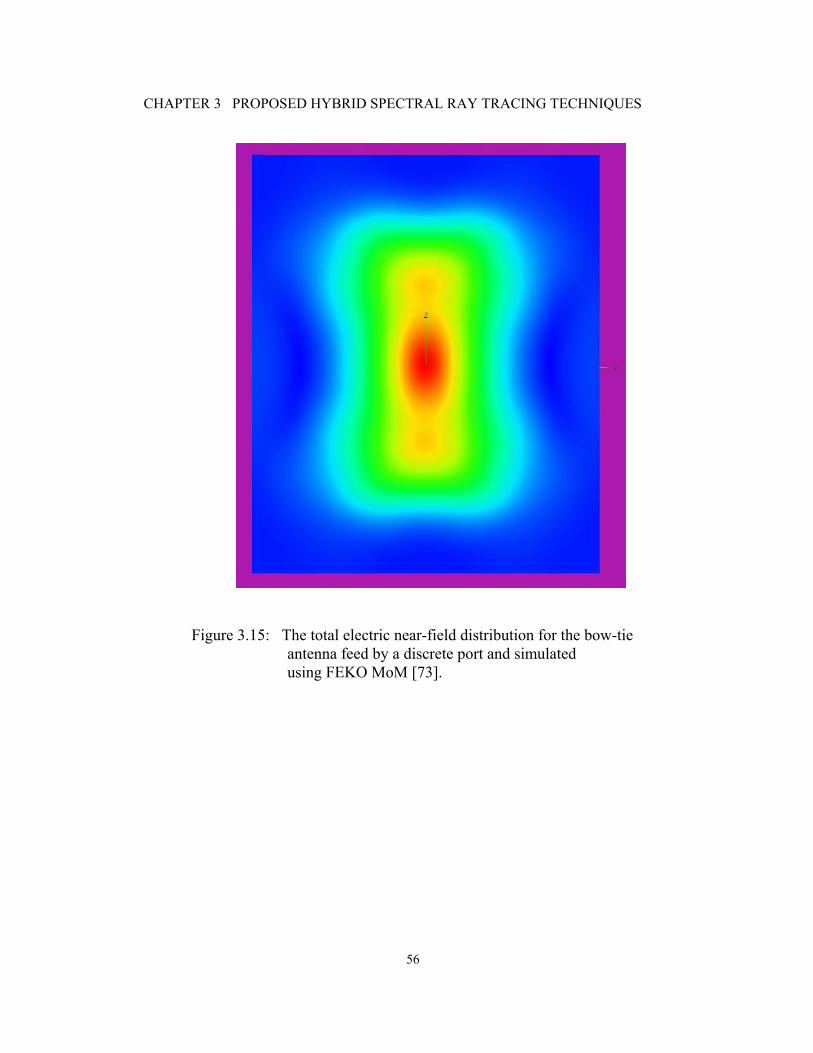
CHAPTER 3 PROPOSED HYBRID SPECTRAL RAY TRACING TECHNIQUES
56
Figure 3.15: The total electric near-field distribution for the bow-tie
antenna feed by a discrete port and simulated using FEKO MoM [73].

CHAPTER 3 PROPOSED HYBRID SPECTRAL RAY TRACING TECHNIQUES
57
-40 -30 -20 -10 0 10 20 30 40-40
-35
-30
-25
-20
-15
-10
-5
0
Rad
iatio
n Pa
ttern
in d
B
θ (degrees)
FEM-SRTHFSS FEM
(a)
(b) Figure 3.16: The (a) E-plane far-field, Ex radiation pattern for the bow-tie
antenna backed by Si hyper-hemispherical lens with FEM-SRT and HFSS responses, and (b) the radiation pattern of total E field in polar coordinates from HFSS.
-6.00
-2.00
2.00
6.00
90
60
30
0
-30
-60
-90
-120
-150
-180
150
120

CHAPTER 3 PROPOSED HYBRID SPECTRAL RAY TRACING TECHNIQUES
58
The Application of HSRT: The MoM-SRT Technique Similar to the FEM-SRT method, one first finds the near-field distribution
over the aperture plane using a MoM solver [73] for a bow-tie antenna of finite length and infinitesimal thickness that is placed on a lossless infinite dielectric half-space as in Fig. 3.11. Then employ the HSRT algorithm outlined in Section 3.3.2.
Fig. 3.17 shows the simulation results for the far-field E-plane radiation pattern of the lens antenna backed by a bow-tie antenna using the MoM-SRT hybrid method with the order of reflection of zero, one and two. The response is verified with the Physical Optics (PO) simulation, the MoM simulation, and MLFMM simulation with FEKO[73]. The MoM-SRT and FEM-SRT algorithm are implemented in Matlab, where the observation points are 60 60θ− ≤ ≤ .
-60 -40 -20 0 20 40 60
-30
-25
-20
-15
-10
-5
0
θ (degrees)
Rad
iatio
n P
atte
rn in
dB
MoM-SRT (OR=0)MoM-SRT (OR=2)FEKO MoM-POFEKO MoM
Figure 3.17: The E-plane far-field total electric field radiation pattern in dB of the electric field obtained using MoM-SRT for the R = 5 mm hyper- hemispherical silicon lens ( 11.9rε = , d = 0.84 mm). The simulation includes the application of MoM-SRT hybrid approach for different reflection orders and the simulation results for the Physical Optics (PO), and the Method of Moment (MoM).

CHAPTER 3 PROPOSED HYBRID SPECTRAL RAY TRACING TECHNIQUES
59
The FEKO MoM simulation to find the near-field of the bow-tie antenna in a half-space took a CPU time of 1 hour, 33 minutes and 34 seconds with two processes running in parallel on a PC with an Intel Centrino Duo 2.4 GHz processor and 6 GB of RAM. The near-field and far-field obtained from the aforementioned simulation is used by the PO, the SRT and the MoM to simulate the hyper-hemispherical lens. The FEKO PO simulation of the lens structure took 1 minute and 53 seconds on the same PC with two processes running in parallel. The MoM technique took an additional 19 minutes to simulate the lens structure, while MLFMM took 13 minutes and 31 seconds on the same PC. The HSRT took 4 minutes and 52 seconds for the reflection order of zero and 7 minutes and 47 seconds for the reflection order of 2 on the same PC exploiting GPU parallel processing to obtain the result in Fig. 3.17. For this particular example, the FEKO PO assumes that the lens surface is in the far-field of the antenna, which is valid only for lenses with a large diameter w.r.t. wavelength, and therefore the computation time is fast because only non-evanescent waves have been taken into consideration. The HSRT takes all rays evanescent and non-evanescent into consideration and provides accurate result for wide-range of lens diameter. The HPBW is 12 degrees.
Table 3.2 shows the comparison between the L2 norm difference of side-lobe levels obtained by the various methods. Let
2MoM−E E be the L2 norm
of the difference between E . The normalized magnitude of the total electric
field in the E-plane obtained using the method shown in Table 3.2, and MoME .
MoME is the normalized magnitude of the total electric field in the E-plane obtained using the MoM. Table 3.3 shows the maximum relative error comparison for the various methods.
TABLE 3.2 COMPARISON OF HYBRID-SRT METHOD WITH OTHER METHODS
APPLIED TO THE BOW-TIE ANTENNA EXAMPLE
Method L2 Norm Difference* 2MoM−E E
FEKO MoM 0 FEKO MLFMM 0.00221
FEKO PO 0.05398 MoM-SRT (OR=0) 0.05820 MoM-SRT (OR=1) 0.05823 MoM-SRT (OR=2) 0.04021
* The difference between the side-lobe levels
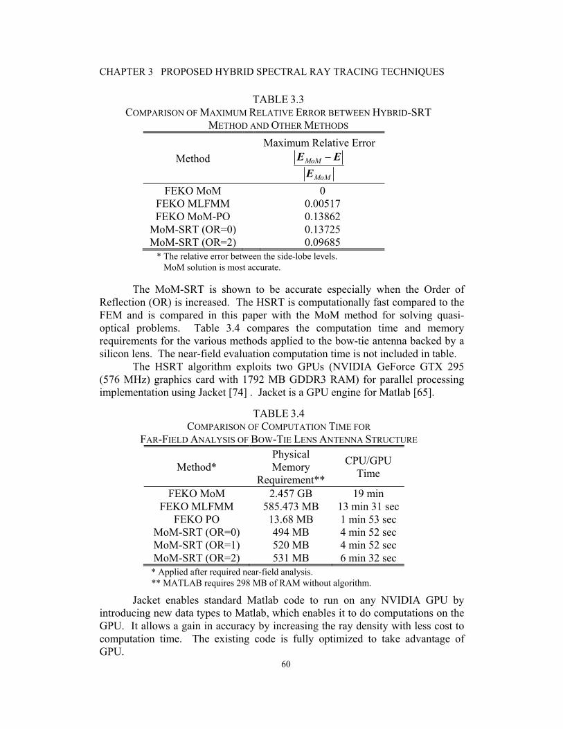
CHAPTER 3 PROPOSED HYBRID SPECTRAL RAY TRACING TECHNIQUES
60
The MoM-SRT is shown to be accurate especially when the Order of Reflection (OR) is increased. The HSRT is computationally fast compared to the FEM and is compared in this paper with the MoM method for solving quasi-optical problems. Table 3.4 compares the computation time and memory requirements for the various methods applied to the bow-tie antenna backed by a silicon lens. The near-field evaluation computation time is not included in table.
The HSRT algorithm exploits two GPUs (NVIDIA GeForce GTX 295 (576 MHz) graphics card with 1792 MB GDDR3 RAM) for parallel processing implementation using Jacket [74] . Jacket is a GPU engine for Matlab [65].
Jacket enables standard Matlab code to run on any NVIDIA GPU by introducing new data types to Matlab, which enables it to do computations on the GPU. It allows a gain in accuracy by increasing the ray density with less cost to computation time. The existing code is fully optimized to take advantage of GPU.
TABLE 3.4 COMPARISON OF COMPUTATION TIME FOR
FAR-FIELD ANALYSIS OF BOW-TIE LENS ANTENNA STRUCTURE
Method* Physical Memory
Requirement**
CPU/GPU Time
FEKO MoM 2.457 GB 19 min FEKO MLFMM 585.473 MB 13 min 31 sec
FEKO PO 13.68 MB 1 min 53 sec MoM-SRT (OR=0) 494 MB 4 min 52 sec MoM-SRT (OR=1) 520 MB 4 min 52 sec MoM-SRT (OR=2) 531 MB 6 min 32 sec
* Applied after required near-field analysis. ** MATLAB requires 298 MB of RAM without algorithm.
TABLE 3.3 COMPARISON OF MAXIMUM RELATIVE ERROR BETWEEN HYBRID-SRT
METHOD AND OTHER METHODS
Method Maximum Relative Error
MoM
MoM
−E EE
FEKO MoM 0 FEKO MLFMM 0.00517 FEKO MoM-PO 0.13862
MoM-SRT (OR=0) 0.13725 MoM-SRT (OR=2) 0.09685
* The relative error between the side-lobe levels. MoM solution is most accurate.
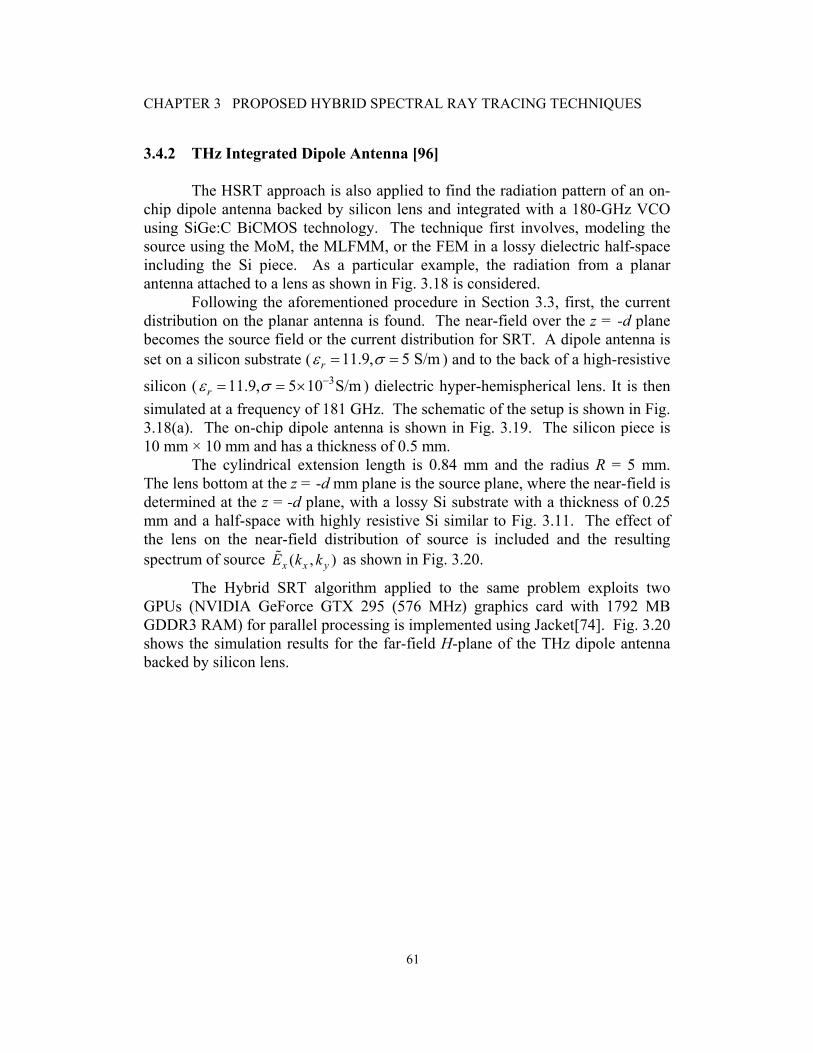
CHAPTER 3 PROPOSED HYBRID SPECTRAL RAY TRACING TECHNIQUES
61
3.4.2 THz Integrated Dipole Antenna [96] The HSRT approach is also applied to find the radiation pattern of an on-
chip dipole antenna backed by silicon lens and integrated with a 180-GHz VCO using SiGe:C BiCMOS technology. The technique first involves, modeling the source using the MoM, the MLFMM, or the FEM in a lossy dielectric half-space including the Si piece. As a particular example, the radiation from a planar antenna attached to a lens as shown in Fig. 3.18 is considered.
Following the aforementioned procedure in Section 3.3, first, the current distribution on the planar antenna is found. The near-field over the z = -d plane becomes the source field or the current distribution for SRT. A dipole antenna is set on a silicon substrate ( 11.9, 5 S/mrε σ= = ) and to the back of a high-resistive
silicon ( 311.9, 5 10 S/mrε σ −= = × ) dielectric hyper-hemispherical lens. It is then simulated at a frequency of 181 GHz. The schematic of the setup is shown in Fig. 3.18(a). The on-chip dipole antenna is shown in Fig. 3.19. The silicon piece is 10 mm × 10 mm and has a thickness of 0.5 mm.
The cylindrical extension length is 0.84 mm and the radius R = 5 mm. The lens bottom at the z = -d mm plane is the source plane, where the near-field is determined at the z = -d plane, with a lossy Si substrate with a thickness of 0.25 mm and a half-space with highly resistive Si similar to Fig. 3.11. The effect of the lens on the near-field distribution of source is included and the resulting spectrum of source ( , )x x yE k k as shown in Fig. 3.20.
The Hybrid SRT algorithm applied to the same problem exploits two GPUs (NVIDIA GeForce GTX 295 (576 MHz) graphics card with 1792 MB GDDR3 RAM) for parallel processing is implemented using Jacket[74]. Fig. 3.20 shows the simulation results for the far-field H-plane of the THz dipole antenna backed by silicon lens.
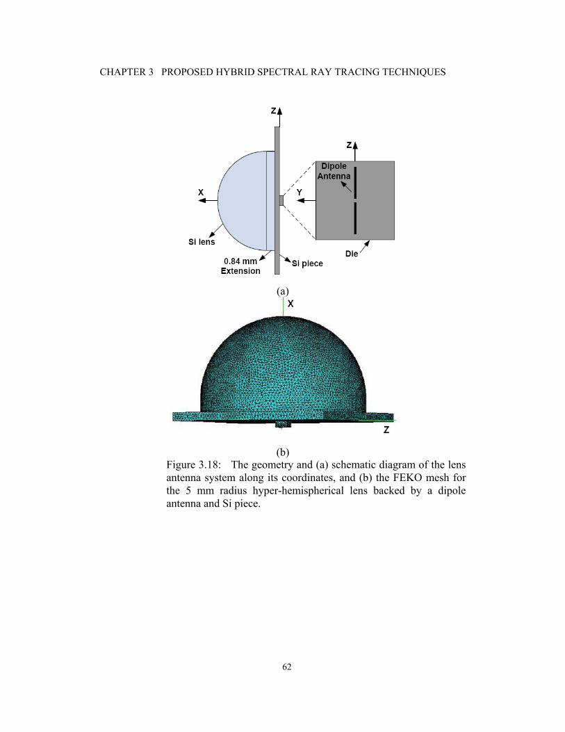
CHAPTER 3 PROPOSED HYBRID SPECTRAL RAY TRACING TECHNIQUES
62
(a)
(b)
Figure 3.18: The geometry and (a) schematic diagram of the lens antenna system along its coordinates, and (b) the FEKO mesh for the 5 mm radius hyper-hemispherical lens backed by a dipole antenna and Si piece.
CHAPTER 3 PROPOSED HYBRID SPECTRAL RAY TRACING TECHNIQUES
63
(a)
(b)
Figure 3.19: (a) A die photo of the fabricated VCO integrated with the on-chip dipole antenna and (b) a transmitter head consists of Si lens and carrier PCB attached to a XY linear stage for precise positioning.

CHAPTER 3 PROPOSED HYBRID SPECTRAL RAY TRACING TECHNIQUES
64
(a)
(b)
Figure 3.20: The spectrum (a) ( , )x x yE k k and (b) ( , )y x yE k k of near-field for the THz dipole antenna backed by Silicon lens. The effect of the lens is included in the near-field distribution. The normalized measured radiation pattern obtained using the Golay cell
is shown in Fig. 3.21. The HSRT result is verified with the MLFMM simulation with FEKO[73], and the measurements the observation points are 20 20φ− ≤ ≤ .

CHAPTER 3 PROPOSED HYBRID SPECTRAL RAY TRACING TECHNIQUES
65
The FEKO MLFMM simulation time was 1.566 hours on a PC with an Intel Dual Core 2.4 GHz processor, 6 GB of RAM, and 2 processes running in parallel.
-20 -15 -10 -5 0 5 10 15 20-30
-25
-20
-15
-10
-5
0
φ (degrees)
Rad
iatio
n P
atte
rn in
dB
Hybrid SRT (OR=0)Hybrid SRT (OR=2)Hybrid SRT (OR=4)FEKO MLFMMMeasurement
Figure 3.21: The Normalized H-plane far-field of the total electric field radiation pattern in dB obtained using the Hybrid MoM-SRT for the R = 5 mm hyper-hemispherical silicon lens ( 311.9, 5 10 S/mrε σ −= = × , d = 0.84 mm). The Radiation pattern measured at 181 GHz and θ=90° plane (Vcc=2.5 V, Vctr=1.6 V). The HSRT ray density was set at 600 along ϕ x 600 along θ for a total of 360,000 rays launched. The simulation included an aluminum metallic back-plate requiring 3.493
GB of RAM. The simulated half-power beam width was 14.1o while it measured at 13.6 degrees. The dipole antenna was aligned so the feed was at the center of the lens. The maximum gain found by simulation was 17.8 dB and the measured gain of the dipole with Si lens antenna is found to be Gt = 17.1 dBi using a superheterodyne setup described in Chapter 5. The HSRT (OR=4) took 8 minutes on the same PC exploiting GPU after finding the spectrum of the near-field distribution using the FEKO MLFMM method in the z=-0.84 mm plane. Fig. 3.22 shows the simulated 3D plot of the antenna gain with and without the Si lens and chip carrier obtained using FEKO.
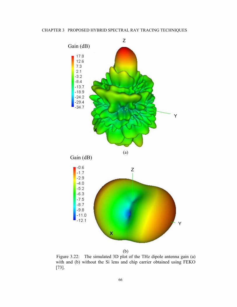
CHAPTER 3 PROPOSED HYBRID SPECTRAL RAY TRACING TECHNIQUES
66
(a)
(b)
Figure 3.22: The simulated 3D plot of the THz dipole antenna gain (a) with and (b) without the Si lens and chip carrier obtained using FEKO [73].
Z
X
Y
Gain (dB)
X
Z
Y
Gain (dB)

CHAPTER 3 PROPOSED HYBRID SPECTRAL RAY TRACING TECHNIQUES
67
3.4.3 THz Integrated Double-Slot Antenna
The twin-slot antennas coupled to CoPlanar Waveguides (CPW) and the double-slot antennas placed at the focus of the dielectric lens are used for quasi-optical detectors that are used in atmospheric and astronomical instruments in the sub-millimeter and THz frequency range. A double-slot antenna is set on the back of a silica ( 3.8rε = ) dielectric hyper-hemispherical lens and simulated at a frequency of 112.5 GHz. The cylindrical extension length is d = R/n, where n = 1.949 is the refractive index and the radius R = 5 mm. The size of the lens was chosen in order to simulate the lens using FEM in Ansoft HFSS [63]. The lens bottom at z = -d mm is a Perfect Electric Conductor (PEC). Fig. 3.23 shows the geometry of the double-slot antenna and the lens. The dimensions of the double-slot antenna are 1.3 mm, 0.7 mm and 40 μm.L S W= = = The electric field distribution in the slot is given by [30]
where 0 00
1 2, = and 2 2
rm
Lk k k yε πλ
+= × ≤ . ( ) 1U x = for interval 2 2,W W−⎡ ⎤⎣ ⎦ .
Fig. 3.24 shows the E-plane radiation pattern and Fig. 3.25 shows the H-
plane radiation pattern for the double-slot antenna. The simulation includes application of the FEM-SRT hybrid approach for different reflection orders and the simulation results for the HFSS FEM, FEKO MoM and SEMCAD FDTD methods. The convergence of the total electric field amplitude and the L2 norm difference between successive E-field iterates is shown in Fig. 3.26.
The reflection order of the rays represents the number of times the rays have been reflected inside the lens. It is seen that the hybrid SRT technique converges to within an error of 10-11 after 14 times reflected rays contribution is considered.
( )20 2
2
sin( ( ))( , , )
sin( )
Lm S
x Lm
k yE x y d E U x
k−
− = × ± (3.37)

CHAPTER 3 PROPOSED HYBRID SPECTRAL RAY TRACING TECHNIQUES
68
(a)
(b)
Figure 3.23: (a) A schematic of a double-slot antenna printed at the back of a hyper-hemispherical lens and (b) the FEKO mesh for the double-slot antenna backed by the lens. The FEM-SRT method is compared with the full HFSS simulation. The
near-field of the aperture plane was found after simulating the slot antenna structure in the dielectric half space using FEM. The FEM HFSS simulation of the double-slot antenna in half-space employing symmetry took 1 minute and 34 seconds on a PC with an Intel Centrino Duo 2.4 GHz processor and 6 GB of RAM. After the near-field in the aperture plane is found, the time taken by the FEM-SRT was 3 minutes and 41 seconds for the reflection order of zero and a ray density of 72,000, and 7 minutes and 31 seconds when the ray density is increased to 720,000. The time taken when the reflection order increases to 2 is 6 minutes

CHAPTER 3 PROPOSED HYBRID SPECTRAL RAY TRACING TECHNIQUES
69
and 32 seconds. The time includes time taken to compute the Fourier transform using LUT and Graphics Processing Unit (GPU). It took 35 min. and 31 sec. with reflection order of 6 and a ray density of 4.32 million. When increasing the ray density from 72 000 to 72 million the norm of the difference between the |E| response of successive iterates is reduced from 4×10⁻⁵ to 3×10⁻⁷.
The FEM HFSS simulation took 8 hours and 56 minutes on the same PC without parallel processing. In Ansoft HFSS, for designs with voltage sources, current sources, or incident waves, ΔW , the difference in the relative scattering energy error between successive adaptive meshing passes for all tetrahedra, is used as the convergence criteria [63]. It measures the stability of the computed field values from iteration to iteration. As the solution converges, ΔW approaches zero. The HFSS solution in Fig. 3.24 and 3.25 converged with a delta energy of ΔW = 0.0043024. The FEKO MoM simulation of the double-slot antenna and lens took 2 hours and 17 minutes with two processes running in parallel and 5.106 GB RAM requirement.
Table 3.5 compares the computation time and memory requirements for the various methods applied to the double slot antenna example. The FEKO MoM, and MLFMM methods were simulated on the same PC with two processes running in parallel. Although the Matlab has overhead in memory, the HSRT methods require much less memory than FEM, MoM and MLFMM, and are comparable in accuracy to these methods. Thus the HSRT methods are computationally fast compared to FEM and MoM for solving electrically large and multi-scale quasi-optical EM problems.
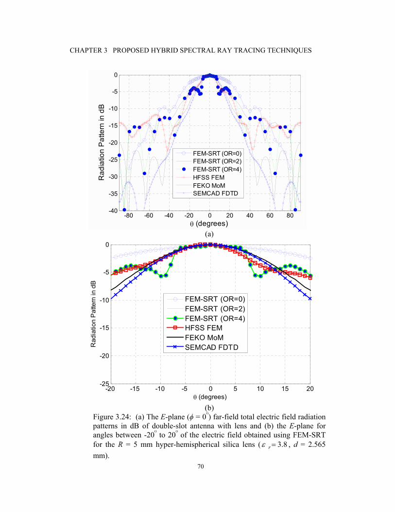
CHAPTER 3 PROPOSED HYBRID SPECTRAL RAY TRACING TECHNIQUES
70
-80 -60 -40 -20 0 20 40 60 80-40
-35
-30
-25
-20
-15
-10
-5
0
θ (degrees)
Rad
iatio
n P
atte
rn in
dB
FEM-SRT (OR=0)FEM-SRT (OR=2)FEM-SRT (OR=4)HFSS FEMFEKO MoMSEMCAD FDTD
(a)
-20 -15 -10 -5 0 5 10 15 20-25
-20
-15
-10
-5
0
θ (degrees)
Rad
iatio
n P
atte
rn in
dB
FEM-SRT (OR=0)FEM-SRT (OR=2)FEM-SRT (OR=4)HFSS FEMFEKO MoMSEMCAD FDTD
(b)
Figure 3.24: (a) The E-plane (ϕ = 0ᴼ) far-field total electric field radiation patterns in dB of double-slot antenna with lens and (b) the E-plane for angles between -20ᴼ to 20ᴼ of the electric field obtained using FEM-SRT for the R = 5 mm hyper-hemispherical silica lens ( 3.8rε = , d = 2.565 mm).

CHAPTER 3 PROPOSED HYBRID SPECTRAL RAY TRACING TECHNIQUES
71
-90 -60 -30 0 30 60 90-40
-35
-30
-25
-20
-15
-10
-5
0
Angle (degrees)
Rad
iatio
n Pa
ttern
in d
B
FEM-SRT (OR=0)FEM-SRT(OR=2)FEM-SRT(OR=4)FEKO MoMHFSS FEM
(a)
-20 -15 -10 -5 0 5 10 15 20-25
-20
-15
-10
-5
0
Angle (degrees)
Rad
iatio
n Pa
ttern
in d
B
FEM-SRT (OR=0)FEM-SRT(OR=2)FEM-SRT(OR=4)FEKO MoMHFSS FEM
(b)
Figure 3.25: (a)The H-plane (ϕ = 90ᴼ) the far-field total electric field radiation patterns in dB of a double-slot antenna with lens and (b) the H-plane for angles between -20ᴼ to 20ᴼ of electric field obtained using FEM-SRT for the R = 5 mm hyper-hemispherical silica lens ( 3.8rε = , d = 2.565 mm).
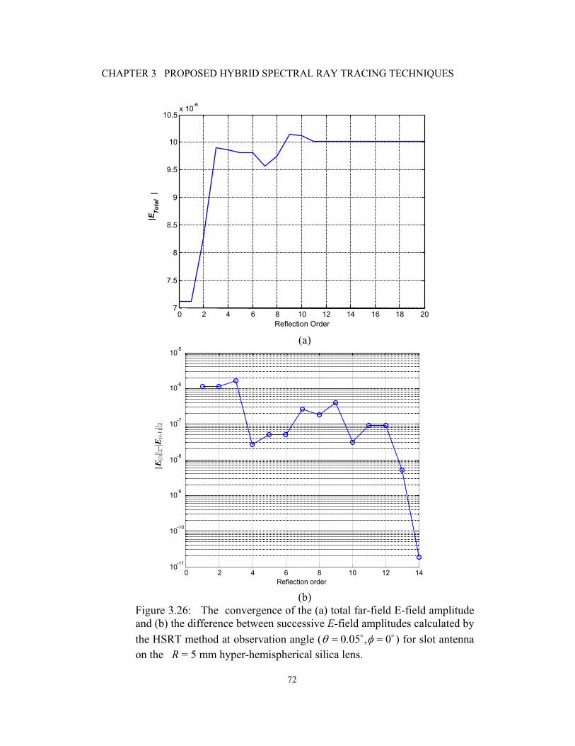
CHAPTER 3 PROPOSED HYBRID SPECTRAL RAY TRACING TECHNIQUES
72
-6
0 2 4 6 8 10 12 14 16 18 207
7.5
8
8.5
9
9.5
10
10.5x 10
Reflection Order
|ETo
tal
|
(a)
0 2 4 6 8 10 12 1410-11
10-10
10-9
10-8
10-7
10-6
10-5
Reflection order
||E(i)
|| 2-|E
(i-1)
|| 2
(b)
Figure 3.26: The convergence of the (a) total far-field E-field amplitude and (b) the difference between successive E-field amplitudes calculated by the HSRT method at observation angle ( 0.05 , 0θ φ= = ) for slot antenna on the R = 5 mm hyper-hemispherical silica lens.

CHAPTER 3 PROPOSED HYBRID SPECTRAL RAY TRACING TECHNIQUES
73
3.5 Spectral Ray Tracing for Modeling Pulse Propagation [92]
Most THz spectroscopic measurements and imaging are done using the
pulsed setup similar to the one shown in Fig. 3.27. In this case, the SRT would have to be formulated for modeling millimeter and THz pulse propagation through a quasi-optical system.
We consider the large-aperture dc-biased terahertz photoconductive antenna shown in Fig. 3.28. The current distribution in the active region of the LTG-GaAs substrate can be modeled as a current sheet. In the presence of a dc bias, the photo-generated carriers in the photoconductor produce a transient surface photocurrent, which radiates an electric pulse with terahertz frequency components in its frequency spectrum into the photoconductor and free space. The hyper-hemispherical silicon lens is then added to prevent the radiation from being trapped inside the photoconducting film by the total reflection [77].
TABLE 3.5 COMPARISON OF COMPUTATION TIME FOR
FAR-FIELD ANALYSIS OF DOUBLE-SLOT LENS ANTENNA STRUCTURE
Method Physical Memory
Requirement** CPU/GPU Time
FEKO MoM 5.106 GB 2 hours 17 min HFSS FEM 8.74 GB 8 hours 56 min
FEKO MLFMM 594 MB 15 min 55 sec FEKO PO 16.53 MB 3 min 07 sec
FEM-SRT (OR=0) 516 MB 3 min 41 sec FEM-SRT (OR=2) 519 MB 6 min 32 sec FEM-SRT (OR=4) 586 MB 9 min 52 sec ** MATLAB requires 298 MB of RAM without algorithm.

CHAPTER 3 PROPOSED HYBRID SPECTRAL RAY TRACING TECHNIQUES
74
Figure 3.27: The experimental setup for the Pulsed/CW measurement of the THz link, the Tx is a bow-tie antenna backed by Si hyper-hemispherical lens and the Rx is a dipole antenna backed by Si hyper-hemispherical lens.
DCV+
DCV−
( )s tJ
y
x
Figure 3.28: A large-aperture dc-biased terahertz photoconductive antenna placed on a hyper-hemispherical silicon lens and excited by a short pulse laser. V is the applied bias voltage and sJ is the induced surface current.

CHAPTER 3 PROPOSED HYBRID SPECTRAL RAY TRACING TECHNIQUES
75
The generated traveling-wave photocurrent can be modeled as a current sheet at z = 0 flowing in the direction of the DC bias electric field and be written as:
where ( )p t is the terahertz pulse generated by illuminating the photoconductor by a laser. The generated surface photocurrent, ( )s tJ , can be represented in terms of the equivalent surface conductivity, ( )s tσ , the dc bias electric field, dcE , and the electric near-field in the LTG-GaAs substrate, ( )near tE , as shown: [78]
where e is the electron charge, and nμ and pμ are the field-dependent electron, and the hole mobilities N(t) and P(t) are the electron and hole concentrations, respectively. In [78], it was found that the radiated field from a large-aperture terahertz photoconductive antenna, placed on a hyper-hemispherical silicon lens and excited by a short pulse laser is saturated when the photo-conductivity exceeds a threshold value defined by the permittivity of the photoconductor material.
The extension of modeling the integrated lens antenna system involves modeling the THz communication link. There, a THz pulse is generated using a femtosecond laser interacting with a photoconductor such as a LTG-GaAs, and propagating through free-space. Since the lens or complex structure media interacting with the antenna are linear, the solution and ray tubes obtained by SRT for a particular structure can be interpreted as the transfer function of the structure. The transfer function of the structure can then be re-used for the analysis of multi-antenna systems, or for different frequencies to simulate pulse propagation. The aim of this component of the research would be to formulate the SRT algorithm for the pulse propagation and model the hyper-hemispherical lens. The measurement setup has a bow-tie transmitter antenna, which was presented in Section 3.4.1 and the receiver is an 80 μm dipole antenna with a 6 μm gap on a 625μm GaAs substrate backed by a 10 mm hyper-hemispherical lens. The proposed hybrid SRT approach along with the new formulation would be used to find the near-field in the source plane and then in free-space.
In this section, the Spectral Ray Tracing (SRT) method was formulated for a pulsed system to model the Terahertz (THz) propagation of a pulse through a lens antenna system. A large-aperture dipole antenna example is then used to
0 ˆ( , ) ( ) ( )s t J z p t xδ=J r (3.38)
( )
0
( ) ( ) ( )
( ) ( ) ( ) ( )
s s dc near
zs n p
t t t
et t e dz N t P tα
σ
σ σ μ μα
∞−
= +
⎡ ⎤= = +⎣ ⎦∫
J E E
(3.39)
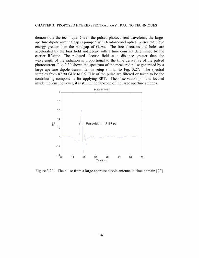
CHAPTER 3 PROPOSED HYBRID SPECTRAL RAY TRACING TECHNIQUES
76
demonstrate the technique. Given the pulsed photocurrent waveform, the large-aperture dipole antenna gap is pumped with femtosecond optical pulses that have energy greater than the bandgap of GaAs. The free electrons and holes are accelerated by the bias field and decay with a time constant determined by the carrier lifetime. The radiated electric field at a distance greater than the wavelength of the radiation is proportional to the time derivative of the pulsed photocurrent. Fig. 3.30 shows the spectrum of the measured pulse generated by a large aperture dipole transmitter in setup similar to Fig. 3.27. The spectral samples from 87.90 GHz to 0.9 THz of the pulse are filtered or taken to be the contributing components for applying SRT. The observation point is located inside the lens, however, it is still in the far-zone of the large aperture antenna.
0 10 20 30 40 50 60 70-0.4
-0.2
0
0.2
0.4
0.6
0.8
1Pulse in time
X(t)
Time (ps)
→ ← Pulsewidth = 1.7167 ps
Figure 3.29: The pulse from a large aperture dipole antenna in time domain [92].

CHAPTER 3 PROPOSED HYBRID SPECTRAL RAY TRACING TECHNIQUES
77
0 0.5 1 1.5 2 2.50
0.005
0.01
0.015
0.02
0.025
0.03
0.035
0.04Spectrum of x(t)
frequency (THz)
|X(f)
|
→ ← Bandwidth = 0.42501 THz
Figure 3.30: The spectrum of the pulse from a large aperture dipole antenna in the frequency domain.
0 0.1 0.2 0.3 0.4 0.5 0.6 0.7 0.8 0.9-180
-120
-60
0
60
120
180
frequency (THz)
Pha
se in
deg
rees
Figure 3.31: The phase in angles of the signal for the range from 87.90 GHz to 0.9 THz of the pulse from a large aperture dipole antenna.

CHAPTER 3 PROPOSED HYBRID SPECTRAL RAY TRACING TECHNIQUES
78
In the past, SRT had been implemented for the continuous wave simulation of electrically large antenna structures. Since SRT is efficient in finding the accurate E-field and radiation pattern at a specified frequency, it was employed to formulate a technique applicable to a pulse source propagating through a lens structure. A number of relevant frequencies from the spectrum of the source are used to find the current distribution or near-field distribution using the dielectric half-space and the planar antenna. The current distribution or the near-field distribution can be used for simulating the SRT at the specific frequencies. The aim is to develop a technique that would efficiently utilize parallel processing and SRT. The electric field including the phase in the time domain at observation point O(x,y,z) is:
Step 1 Given the spectrum of the source pulse p(t); find the significant ranges of frequencies to sample that contribute to the pulse. If the pulse is given in time domain, take the Fourier transform and store the n complex number samples. For example, the spectral samples from 87.90 GHz to 0.8 THz are used with n = 50 for the simulation.
Step 2 The planar antenna structure using a half-space is simulated using MoM or FEM for each frequency, with a voltage source of an amplitude of 1V to find the near-field distribution at the boundary between the lens and substrate. (During implementation, this is done in parallel).
Step 3 Apply SRT using the near-field distribution for the source with 0 1 V/mE = .
Step 4 Take the inverse Fourier transform of n contributions with the complex amplitude.
Spectral Ray Tracing Formulation for Pulse Propagation
Given the near-field distribution ( , , , )x y d ω−E over the aperture plane z = -d, for each sample frequency ω :
The 2D Fourier transform is calculated to get ( , )x x yE k k and ( , )y x yE k k
( , , ) ˆ ˆ ˆ( ) ( ) ( )O x y z x y zE t E t E t= + +E x y z (3.40)
ˆ ˆ ˆ( , , , ) ( , , ) ( , , ) ( , , )x y zx y d E x y d E x y d E x y dω− = − + − + −x y zE (3.41)

CHAPTER 3 PROPOSED HYBRID SPECTRAL RAY TRACING TECHNIQUES
79
First backward-ray launching is applied to determine the ray paths from the initial Plane Wave Spectrum (PWS) through O. We then applied a different technique than the one used in the past to determine the corresponding complex field amplitudes for each ray as we considered the pulse. In order to do backward-ray launching, we calculated max ,d and dφ φ θ as a function of the Order of Reflection (OR). Then set miniφ φ= and 1id dφ φ= . If these TPRs depart the z=-d plane, instead of calculating the field created by the TPRs for a single frequency, we found the p partial vectors with a complex magnitude:
where
and ,( , )p m nDFω is the total divergence factor calculated for an angular frequency
pω . The Fourier transform of the pulse source was given by:
Using the property *( ) ( )X f X f= − , we obtained the frequencies spectrum as in Fig. 3.30. Taking the normalized signal ( )X f in dB and only considering the signals that are above -45 dB, we obtained the complex amplitude and phase for the range 87.90 GHz to 0.8207 THz. At p frequencies we have:
( )2
1( , ) ( , , )4
x yj k x k yx x y xE k k E x y d e dxdy
π+∞ +∞ +
−∞ −∞= −∫ ∫ (3.42)
( , ) ( , )( , ) x x y x y x y y
z x yz
E k k k E k k kE k k
k+
= (3.43)
() , ,( , )
, ( , , )
, ,( , ) , ,( , )
2, ,( , ) ,( , ) , ,( , )
ˆ ˆ ˆ
ˆ ˆ ( ) ( )
ˆ ( )
p
p p
t m npp p p
O x y z x y z
x t m n y t m nm n
jz t m n m n t m n
E E E
E E
E DF d e ω
ω
ω ω
ω ω ω− ⋅
= + +
= +
+ ⋅ ⋅ ⋅
∑∑k r
E x y z
k x k y
k z k
.
(3.44)
2
2, ,( , ) sin(2 )
2pp
t m n n n mk
d d dω θ θ φ=k (3.45)
( ) ( ) exp( 2 )X f x t j ft dtπ∞
−∞
= −∫ . (3.46)

CHAPTER 3 PROPOSED HYBRID SPECTRAL RAY TRACING TECHNIQUES
80
Applying the convolution,
where
Going back to the example of the large-aperture photoconductive antenna, assume the pulse p(t) in Eq. (3.38) is known and take one frequency component of the spectrum j te ω , applying the boundary conditions, the aperture distribution to be in the plane z=0 [79],
Here the 0η is the intrinsic impedance of free space and rε is the relative dielectric constant of the photoconductor. The corresponding plane wave spectrum becomes
And
where a= 10 mm and the gap b=5 mm.
( ) ( ) pjp pX f X f e ϕ= . (3.47)
1
( , , ) 1 , ( , , )0
( ) ,
for 0,1, , 1
p pp
Nj j n t
O x y z n O x y z pp
t X e e
n N
ϕ ωω
−Δ
+=
= ⋅
= −
∑…
E E
(3.48)
2
pp
N tπω =Δ
. (3.49)
0 0
r
( ) | | and | |1+( , )
0 elsewherex
J x a y bE x y
η ωε
−⎧ ≤ ≤⎪= ⎨⎪⎩
(3.50)
02
sin( )sin( )( , ) yxx x y
x y
k bE ab k aE k kk a k bπ
= × × (3.51)
02 2 2 2
sin( )sin( )( , )( )
yxz x y
yx y
k bE ab k aE k kk bk k k aπ
= − × ×− −
(3.52)

CHAPTER 3 PROPOSED HYBRID SPECTRAL RAY TRACING TECHNIQUES
81
Figures 3.32 and 3.33 show the far-field electric field response in the time domain at the observation point, with a distance of 61 cm. This is due to large-aperture dc-biased terahertz photoconductive antenna placed on hyper-hemispherical silicon lens. Figures 3.34 and 3.35 show the SRT simulated the far-field radiation pattern for the 4 mm by 5 mm aperture at 87.9336 GHz and 102.5892 GHz. The simulated radiation pattern obtained using SRT for the THz photoconductive antenna with a 4 mm by 1 mm aperture size is shown in Figures 3.36 to 3.37. This is followed by the far-field electric field in the time domain as simulated at different observation angles as shown in Fig. 3.38. The attenuation of the pulse and the pulse shape distortion, such as the observation angle is changed from broadside, is similar to the measurements of the radiation pattern for a bow-tie with 90 degree opening angle [71]. The simulated directivity is shown in Fig. 3.39.
0 10 20 30 40 50 60 70-15
-10
-5
0
5
10
time (ps)
Ex(t)
(kV
/cm
)
Figure 3.32: The far-field Ex electric field in the time domain at the observation point ( , , ) (61 ,0 ,0 )r cmθ φ = is due to large-aperture dc-biased terahertz photoconductive antenna placed on a hyper-hemispherical silicon lens excited by a short pulse laser.

CHAPTER 3 PROPOSED HYBRID SPECTRAL RAY TRACING TECHNIQUES
82
0 10 20 30 40 50 60 70-5
-4
-3
-2
-1
0
1
2
3
4
time (ps)
Ex(t)
(kV
/cm
)
Figure 3.33: The far-field Ex electric field in the time domain at the observation point ( , , ) (61 , 20 ,0 )r cmθ φ = due to a large-aperture dc-biased terahertz photoconductive antenna placed on a hyper-hemispherical silicon lens excited by a short pulse laser.

CHAPTER 3 PROPOSED HYBRID SPECTRAL RAY TRACING TECHNIQUES
83
0 5 10 15 20 25 30 35 40-30
-25
-20
-15
-10
-5
0
Rad
iatio
n P
atte
rn in
dB
theta (degrees)0 5 10 15 20 25 30 35 40
-180
-90
0
90
180
Pha
se in
Deg
rees
Figure 3.34: The E-plane far-field, Ex, radiation pattern in dB and the phase of
the electric field obtained using SRT for the R = 5 mm Si ( 11.9rε = ) hemispherical lens backed by a large-aperture dc-biased terahertz photoconductive antenna at 87.9336 GHz.
0 5 10 15 20 25 30 35 40-30
-25
-20
-15
-10
-5
0
Rad
iatio
n P
atte
rn in
dB
theta (degrees)0 5 10 15 20 25 30 35 40
-180
-90
0
90
180
Pha
se in
Deg
rees
Figure 3.35: The E-plane far-field, Ex, radiation pattern in dB and the phase of
electric field obtained using SRT for the R = 5 mm hemispherical lens with 11.9rε = for a large-aperture dc-biased terahertz photoconductive antenna at 102.5892 GHz.

CHAPTER 3 PROPOSED HYBRID SPECTRAL RAY TRACING TECHNIQUES
84
Next we consider a large aperture dipole antenna with aperture dimensions of 4 mm × 1 mm.
0 5 10 15 20 25 30 35 40-30
-25
-20
-15
-10
-5
0
Rad
iatio
n P
atte
rn in
dB
theta (degrees)0 5 10 15 20 25 30 35 40
-180
-90
0
90
180
Pha
se in
Deg
rees
Figure 3.36: The E-plane far-field, Ex, radiation pattern in dB and the phase of
the electric field obtained using SRT for the R = 5 mm hemispherical lens with 11.9rε = for a large-aperture (4 mm × 1 mm) dc-biased terahertz photoconductive antenna at 87.9336 GHz.
0 5 10 15 20 25 30 35 40-30
-25
-20
-15
-10
-5
0
Rad
iatio
n P
atte
rn in
dB
theta (degrees)0 5 10 15 20 25 30 35 40
-180
-90
0
90
180P
hase
in D
egre
es
Figure 3.37: The E-plane far-field, Ex, with the radiation pattern in dB and the
phase of the electric field obtained using SRT for the R = 5 mm hemispherical lens with 11.9rε = for a large-aperture (4 mm × 1 mm) dc-biased terahertz photoconductive antenna at 102.5892 GHz.

CHAPTER 3 PROPOSED HYBRID SPECTRAL RAY TRACING TECHNIQUES
85
Figure 3.38: The E-plane far-field, Ex in the time domain obtained using SRT for
the R = 5 mm hemispherical lens with 11.9rε = for a large-aperture (4 mm × 1 mm) dc-biased terahertz photoconductive antenna at different angles of observation [92].
0 0.1 0.2 0.3 0.4 0.5 0.6 0.7 0.8 0.932
34
36
38
40
42
44
46
frequency (THz)
Dire
ctiv
ity (d
B)
Figure 3.39: The directivity vs. frequency for the E-plane far-field.

CHAPTER 3 PROPOSED HYBRID SPECTRAL RAY TRACING TECHNIQUES
86
3.6 Limitations of HSRT
The HSRT algorithm assumes the electrically large region to be modeled using SRT is smooth and refractive index continuous without edges. The HSRT algorithm in its present form can not model electrically abrupt discontinuities such as wedges, but by applying GTD to spectral rays we can model wedges and edges. The HSRT method assumes Eq. (3.1) to (3.3) hold for the spectrum of the source, e.g. we are dealing with a charge-free region.
The HSRT algorithm is applicable, similar to SRT, for size of the analyzed objects in terms of wavelength of a few wavelength and up. If the size of the lens or object to be analyzed is below 3λ, then for HSRT to work we have to introduce complex rays [16][17] which makes the ray tracing more complex. So for sizes less than a few wavelength, it is recommended to use rigorous numerical solvers.
3.7 Conclusions
In this chapter, I describe and present a computationally efficient self-consistent Hybrid Spectral Ray Tracing (HSRT) methods, MoM-SRT, FEM-SRT and MLFMM-SRT, which require one spectral domain integration step for each observation point. The MLFMM-SRT and MoM-SRT methods are compared with measurements and commercially available Method of Moments (MoM) software, Multi-level Fast Multipole Method (MLFMM) AND Physical Optics (PO) via simulation of a bow-tie terahertz antenna backed by hyper-hemispherical silicon lens and an on-chip dipole lens antenna. The E-plane radiation pattern of an edge-coupled traveling-wave photomixer integrated with a bow-tie antenna backed by a hyper-hemispherical lens was obtained using the MoM-SRT method. HSRT method is also applied to an on-chip planar THz dipole antenna lens structure integrated with a VCO fabricated in SiGe:C BiCMOS technology. The use of GPU parallel processing greatly accelerates computational time of HSRT and SRT.
In Chapter 4, the method for gain measurement and experimental setup for the on-chip dipole antenna and lens system is presented. In this method, the radiation pattern is first measured in a quasi-optical configuration using a power detector. Subsequently, the radiated power is estimated from the integration over the radiation pattern. The antenna gain is obtained from measurement of a two-antenna system. The experimental results of applying this method on an on-chip planar dipole attached to a hyper-hemispherical silicon lens are demonstrated.

87
CHAPTER 4
The Experimental Setup for the Antenna
Characterization of an Embedded On-chip
Antenna in the mmW/THz Range
The on-chip antenna simplifies the packaging and eliminates the pad and
bonding parasitics from the high frequency nodes of the circuit such as the receiver input and the transmitter output, and it improves the system performance. However, the major challenge is the characterization of such on-chip antennas at the mmW/THz range of frequency. The waveguide based wafer prober is more or less a common setup for this type of measurement, and is now available commercially for frequencies below 500 GHz even though the instrument may be quite expensive and not accessible to many groups.
In this chapter, a simple method for the gain measurement of an embedded antenna is presented. The experimental results from applying this method on an on-chip planar dipole integrated with a 180-GHz VCO in SiGe:C BiCMOS technology, and attached to a hyper-hemispherical silicon lens is demonstrated. In the method, first, the radiation pattern is measured using a high sensitivity power detector or Golay Cell. Subsequently, the radiated power is estimated from the integration over the radiation pattern. Then, the antenna gain is measured in a two-antenna system using an open-ended waveguide as the receiving antenna, and a spectrum analyzer and harmonic mixer as the receiver.
4.1 Antenna Design and Simulations [97]
Fig. 4.1 shows the schematic of a planar dipole antenna connected to a Voltage Control Oscillator (VCO) via a transmission line integrated on a single chip. The oscillator was designed for the target frequency of around 180 GHz and tuning range of 5 GHz. The output of the VCO is differential with the impedance

CHAPTER 4 EXPERIMENTAL SETUP for ANTENNA CHARACTERIZATION of EMBEDDED ON-CHIP ANTENNA in mmW/THz RANGE
88
Figure 4.1: The schematic of a dipole antenna connected to a VCO via transmission line.
of 100 Ω. The circuits were designed in 0.13 µm using SiGe:C BiCMOS technology from IHP with npn-HBTs featuring fT /fmax=250/300 GHz.
The dipole antenna was designed on a silicon substrate with the thickness of 250 µm and a resistivity of 20 Ω-cm. The substrate then, is attached from the back side to a high resistivity hyper-hemispherical silicon lens with a radius of 5 mm and an extension of 0.84 mm to reduce the loss due to the surface wave modes in the substrate, and to increase the antenna gain.
For the initial design of the half-wavelength dipole, the silicon lens attached to the antenna substrate can be approximated by a half-space medium, since its radius is large compared to the wavelength (by almost 10 times). This approximation enables one to use the Method of Moment (MoM) as a fast and full-wave design tool for optimizing the geometry of the planar dipole based on the input impedance and resonance frequency requirements
Fig. 4.2 shows the simulated input return loss of the optimized planar dipole on half-space silicon obtained from MoM using ADS Momentum (a commercial EM simulator). As seen in Fig. 4.2, the bandwidth at 10 dB return loss of100 GHz and around center frequency of 220 GHz. In this simulation, the width and total length of the dipole are 20 µm and 345 µm, respectively, and the feeding transmission line is CoPlanar Strip (CPS) with the width and spacing of 10.4 µm and 10.0 µm, respectively. The metal strip is made from 2µm-thick aluminum. Besides substrate loss, a loss tangent of 0.001 is also considered for the half-space.
Although half-space approximation gives fairly accurate results for the input impedance of the antenna, the geometry of the silicon lens should be included in the simulations for the study of far-field characteristics such as the radiation pattern.

CHAPTER 4 EXPERIMENTAL SETUP for ANTENNA CHARACTERIZATION of EMBEDDED ON-CHIP ANTENNA in mmW/THz RANGE
89
Figure 4.2: Simulated input return loss of the planar dipole on half-space silicon. For a fast analysis of the combined planar dipole and silicon lens, we
apply the HSRT method outlined in Chapter 3. The advantage of the HSRT method is that it can be applied for an arbitrary large complex structure very efficiently.
Applying the Hybrid SRT algorithm for the structure shown in Fig. 3.18(a), the configuration of the chip substrate attached to the silicon lens through a high resistive silicon piece that is 10 mm × 10 mm with a thickness of 0.5 mm, and a known field at the source plane. The Si piece is used as the carrier for easy handling of the chip. The chip substrate size is 0.8 × 0.6 mm2 and the thickness is 0.25 mm. Fig. 3.21 shows the normalized far-field distribution (radiation pattern) in the H-plane. The ray density in the HSRT method was set to (600 along ϕ x 600 along θ) for a total of 360,000 rays launched. In Fig. 3.21 the results for 0, 2nd and 4th orderof multiple-reflection are compared. Increasing the order to more than 4 has a small impact on the radiation pattern because of the dielectric loss. In Fig. 3.21, the results obtained from HSRT are also compared with those obtained from the Multilevel Fast Multipole Method (MLFMM) using FEKO[73] and is also a measurement result.
Fig. 3.22(a) shows the simulated 3D plot of the antenna gain with the Si lens and chip carrier obtained using FEKO. The maximum directivity and gain are 20.85 dB and 17.80 dB, respectively, along the z-axis. The radiation efficiency is calculated to be around 49.55%. Fig. 3.22(b) shows the simulated 3D

CHAPTER 4 EXPERIMENTAL SETUP for ANTENNA CHARACTERIZATION of EMBEDDED ON-CHIP ANTENNA in mmW/THz RANGE
90
plot of the antenna gain without the Si lens and chip carrier obtained using FEKO. In this case, the maximum directivity and gain are 3.6 dB and -0.6 dB, respectively, whereas the gain along z-axis is calculated as -7.5 dB. The radiation efficiency without the silicon lens is around 38%. It is evident from Fig. 3.23 that the impact of the silicon lens on the improvement of the gain and radiation efficiency is considerable.
4.2 Measurement Approach
Fig. 3.19(a) shows a photo of the fabricated chip. It includes a VCO integrated with a planar dipole antenna through the CPS transmission line. The silicon piece is attached to a carrier PCB, where the bias and control voltage pads on the chip are wire bonded to the PCB terminals.
To have precise control over the position of the chip during the alignments, the PCB board is attached to an XY linear translation stage as shown in Fig. 3.19(b). After that the silicon lens sits on the backside, and a second translation stage (not shown) is used to slide the Si lens against the Si piece very precisely. Using two translation stages gives the flexibility of adjusting the chip and silicon lens independently.
We characterized the on-chip antenna using both the quasi-optical and superheterodyne setups.
4.2.1 Quasi-optical Setup Fig. 4.3 illustrates a schematic of the quasi-optical setup along with a
photo of the lab setup. In the setup, the transmitter head is placed on a rotational stage which facilitates the measurement of the radiation pattern.
The radiated field from the on-chip dipole is coupled to the free space through the silicon lens. A bi-convex spherical lens collects and focuses the incoming beam on the input aperture of a Golay cell. The Golay Cell is an optoacoustic power detector featuring a very high sensitivity and a wide spectrum range of 0.02-20 THz. It is equipped with a 6 mm diameter polyethylene input window that provides high transparency at frequencies up to 20 THz. The bi-convex spherical lens is made of polished Tsurupica with the clear aperture of 45 mm and a focal length of 50 mm.
To block the thermal radiation generated by the DC power dissipation in the device (Vcc = 2:5 V; Icc = 30 mA), a THz low pass filter is placed in front of the focusing lens. The THz low-pass filtering window gives above a 95% transmission at the mm-wave range whereas the transmission reduces to below 0.1% at IR range.

CHAPTER 4 EXPERIMENTAL SETUP for ANTENNA CHARACTERIZATION of EMBEDDED ON-CHIP ANTENNA in mmW/THz RANGE
91
(a)
(b)
Figure 4.3: (a) The schematic diagram of the quasi-optical setup (b) The quasi-optical test bench.[97] A mechanical chopper placed right after the transmitter head modulates
the beam at a 20 Hz chopping frequency. The output voltage of the Golay cell is detected by a lock-in amplifier with a reference signal synchronized with a chopping frequency. Using the lock-in amplifier substantially reduces the interference due to ambient radiations.
Using the quasi-optical setup and by having the responsivity of the Golay cell, the received power at the Golay cell was measured to be around -15.7 dBm (27 µW) which includes all the transmission losses of the components along the propagation path. It should be noted that in the alignments, the height and the azimuthal orientation of each component, the position of the device, the silicon lens and the location of the Golay cell were carefully optimized for obtaining the maximum detected power. Next to the radiated power estimation, the radiation

CHAPTER 4 EXPERIMENTAL SETUP for ANTENNA CHARACTERIZATION of EMBEDDED ON-CHIP ANTENNA in mmW/THz RANGE
92
pattern of the planar dipole with a silicon lens was measured by a quasi-optical setup as shown in Fig. 3.21.
In the quasi-optical setup, the ratio between the received power by the Golay cell, Pr, and the total radiated power from the transmitting antenna, Pt, is given as:
where F(ϕ, θ) is the normalized measured radiation pattern using the Golay cell. The solid angle for the portion of the power captured by the Golay cell, 0Ψ , is calculated from the geometry of the setup and the clear aperture of the focusing lens. The ratio is found after the integration in Eq. (5.1) to be 0.73. Since the received power was measured Pr = 27 µW, the total radiated power is estimated to be Pt = 37.2 µW or -14.3 dBm.
4.2.2 The Superheterodyne Setup
Fig. 4.4 illustrates a schematic of the superheterodyne setup along with a photo of the lab setup. In this setup, the transmitter head is placed in front of an open aperture of a WR-5 rectangular waveguide through which the coupled radiation is transmitted to a Harmonic Mixer (the M05HWD model from Oleson Microwave Labs (OML)) as the RF signal. The RF frequency of the harmonic mixer can be in the range of 140-220 GHz, and is down converted to an IF frequency with a LO frequency up to 18.6 GHz. The nominal LO power level is specified as 12-15 dBm. The Input LO signal and the output IF signal in the harmonic mixer shares the same SMA connector, and are separated by an external diplexer. The external diplexer is connected to the harmonic mixer through a coaxial cable. We used a PSA spectrum analyzer (E4448A model from Agilent) to monitor the signal spectrum. The PSA spectrum analyzer has the external mixing option to extend the measurement frequency up to 325 GHz, and provide a LO signal (3.05-6.89 GHz, up to +20.5 dBm) and a bias current (±10 mA) for the harmonic mixer.
Fig. 4.5 shows the measured spectrum of the received signal. The spectrum shows a signal with the center frequency of 181.5 GHz and a -88.8 dBm power. It should be noted that the conversion loss of the harmonic mixer (≈55 dB) is included in the power reading.
0
4
( , )
( , )r
t
F dPP F d
π
φ θ
φ θΨ
Ψ
=Ψ
∫
∫
(5.1)

CHAPTER 4 EXPERIMENTAL SETUP for ANTENNA CHARACTERIZATION of EMBEDDED ON-CHIP ANTENNA in mmW/THz RANGE
93
(a)
(b)
Figure 4.4: (a) The schematic diagram of the superheterodyne setup (b) The superheterodyne test bench.[97]
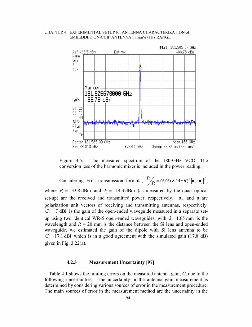
CHAPTER 4 EXPERIMENTAL SETUP for ANTENNA CHARACTERIZATION of EMBEDDED ON-CHIP ANTENNA in mmW/THz RANGE
94
Figure 4.5: The measured spectrum of the 180-GHz VCO. The conversion loss of the harmonic mixer is included in the power reading.
Considering Friis transmission formula, 22( / 4 )rr t r t
t
P G G RP λ π= ⋅a a ,
where 33.8 dBmrP = − and 14.3 dBmtP = − (as measured by the quasi-optical
set-up) are the received and transmitted power, respectively. ra and ta are polarization unit vectors of receiving and transmitting antennas, respectively.
7 dBirG = is the gain of the open-ended waveguide measured in a separate set-up using two identical WR-5 open-ended waveguides, with
1.65 mmλ = is the
wavelength and R = 20 mm is the distance between the Si lens and open-ended waveguide, we estimated the gain of the dipole with Si lens antenna to be
17.1 dBitG = which is in a good agreement with the simulated gain (17.8 dB) given in Fig. 3.22(a).
4.2.3 Measurement Uncertainty [97]
Table 4.1 shows the limiting errors on the measured antenna gain, Gt due to the following uncertainties. The uncertainty in the antenna gain measurement is determined by considering various sources of error in the measurement procedure. The main sources of error in the measurement method are the uncertainty in the

CHAPTER 4 EXPERIMENTAL SETUP for ANTENNA CHARACTERIZATION of EMBEDDED ON-CHIP ANTENNA in mmW/THz RANGE
95
calibration of the power meter in the quasi-optical setup, uncertainty in the gain accuracy of the receiving antenna in the superheterodyne setup. There is also uncertainty in the harmonic mixer characteristics such as conversion loss and RF input return loss, uncertainty in the radiation efficiency of the transmitting antenna, misalignment between two antennas, possible violation of far-field condition, and existence of scattering and multiple reflections in the superheterodyne setup.
4.3 Conclusions
In this chapter, we present a simple method for gain measurement of an embedded on-chip antenna where the feeding network is not accessible. This method only needs a sensitive power detector, and does not depend on expensive instrumentation such as wafer prober and network analyzer in mmW/THz range. The measured gain is compared with simulations on an on-chip planar dipole fabricated in SiGe:C BiCMOS technology and attached to a hyper-hemispherical silicon lens. A radiated power of around 40 µW and measured gain of 17 dB is obtained at 180 GHZ for this antenna structure.
TABLE 4.1 LIMITING ERRORS ON THE MEASURED ANTENNA GAIN Gt
Gr Efficiency ηt ± 5%
Misalignment ± 1o
± 0.1 dB ±0.3 dB ±0.2 dB

96
CHAPTER 5
The Experimental Setup and
Application to the Material Characterization
for Imaging Purposes
A THz imaging modality built upon the coherent THz interactions with a tooth is appealing because the radiation is non-ionizing and unlike X-rays, non-invasive. There are a number of benefits to be offered in dental imaging by a technique that has a high sensitivity to dental caries. Since current techniques do not offer comprehensive information concerning the different types of caries at the required level of sensitivity and specificity. X-ray imaging is not only inadequate, but raises safety concerns for children due to the use of ionizing radiation in regular screening. The dielectric characterization of a tooth from 0.5 to 1.5 THz had been conducted in [76]. The THz application to dental imaging was proposed using a pulsed setup [6]. Since the dielectric characterization measurements of tooth material properties especially those concerning loss is not readily available below 500 GHz in the literature. One of the objectives of this research is to establish the characteristic properties of the enamel and dentine at millimeter-wave and terahertz frequencies. As well as being able to differentiate between the enamel, dentine, pulp, dental caries, and crown. One expects a low absorption of millimeter-waves and THz in tooth material.
The dielectric characterization and the spectroscopic measurements of the different tooth samples, enamel, root dentine, and dental caries that were obtained from a dentist, was conducted for the frequency range from 94.996 GHz to 176.282 GHz using a Backward Wave Oscillator (BWO) in transmission-mode.
HSRT is an effective method for the simulation of the THz (sub-millimeter-wave) imaging, and the characterization setup and processes. The HSRT is compared for the transmission image with the Transmission Line Matrix (TLM) method.
There are pulsed and continuous-wave THz photomixing spectroscopy, and imaging setup using photoconductive a source and detector available at the Microwave and Terahertz Photonics Integrated System Lab (MISL) of CAIRS

CHAPTER 5 EXPERIMENTAL SETUP AND APPLICATION TO MATERIAL CHARACTERIZATION FOR IMAGING PURPOSES
97
(Centre for Intelligent Antenna and Radio Systems). A Backward-Wave Oscillator (BWO) is also available for imaging and spectroscopy. The MISL supports far reaching research in the area of millimeter-wave and THz photonics with an emphasis on the THz applications in the pharmaceutical and life sciences, DNA sequencing, and communications. The high-power Backward-Wave-Oscillator (BWO) and frequency multiplier sources have a range from 95 GHz to1.6 THz with an output power in the range of 1 µW-100 mW. A femto-second short pulse laser that has an average power greater than 2.5 W, a wavelength of 690-1020 nm, with a pulse duration of <100 fs, and 80 MHz repetition rate is used to generate the THz by interacting with a photoconductive antenna for the pulsed spectrometer and imager. Both the electro-optic and photoconductive detection setup are available at the MISL. Fig. 3.27 shows the experimental setup for the pulsed/CW THz spectroscopy and imaging without the sample and focusing lens. For the case of imaging and spectroscopy, a sample holder is placed on a motorized stand at the focus of the two focusing lenses placed between the off-axis mirrors. Other than the mirrors, the following equipment is available for use in the setup:
• Tunable CW laser, with a wavelength of 780 nm ± 10 nm, an output power of 500 mW, with free-space and fiber coupled options
• Femtosecond-short pulse laser, with a wavelength of 690-1020 nm, a pulse duration of <100 fs, a 80 MHz rep rate, and an average power of >2.5 W
• DSP digital lock-in amplifier, with a 1 mHz to 102 KHz frequency range, and >100 dB of dynamic reserve
• Low-noise current amplifier, with a 5 fA/Hz1/2 input noise In this chapter, the BWO is used for the CW spectroscopy and imaging of the polyethylene and tooth biological samples.
5.1 The Experimental Setup for Spectroscopic Measurement In this section, the interaction of the THz wave with the lens, a
polyethylene sample and a biological media such as tooth is considered. The dielectric characterization and spectroscopic measurements of different tooth samples, obtained from a dentist was conducted for the frequency range from 94.996 GHz to 176.282 GHz using backward wave oscillator (BWO) in transmission-mode. Fig. 5.1 shows the schematic of the slab to be measured using BWO. The system is based on a millimeter wave BWO combined with

CHAPTER 5 EXPERIMENTAL SETUP AND APPLICATION TO MATERIAL CHARACTERIZATION FOR IMAGING PURPOSES
98
Figure 5.1: (a) The simplified schematic layout of the slab sample, source
and detector for transmission mode measurements. frequency multipliers and a broadband Pyroelectric detector. The system setup for the measurement was done in consultation with Dr. Daryoosh Saeedkia. I also would like to thank Quantum Dental and Dr. Mitra Doherty for making the tooth samples available for the research.
A backward-wave oscillator-based spectroscopy as shown in Fig. 5.2 is employed to measure the power passing through a sample. Relatively transparent materials were prepared in the form of a flat parallel slab or disc, the transmittance is an oscillating function of the frequency due to multiple reflections of the EM wave on the sample interface. The refractive index can be evaluated from the distance between two maximum points in the wave, and the absorption index can be evaluated from the amplitude of the transmittance level of in the peak. The complex transmittance can be expressed as:
where
2 2
2 2 sample
(1 ) 4 sin(1 ) 4 sin ( )
sample
no
P R RT EP RE RE N
θθ
− += =
− + +
(5.1)
( )
2 2
2 2
2
*
*
( 1)( 1)
4exp
arctan 2 /( 1)
2 /
n kRn k
k dEc
b a b
N nd c
a ib
π ν
θ
π ν
με
− +=
+ +
−⎛ ⎞= ⎜ ⎟⎝ ⎠
= + −
=
⎛ ⎞⎜ ⎟+ =⎜ ⎟⎝ ⎠
(5.2)

CHAPTER 5 EXPERIMENTAL SETUP AND APPLICATION TO MATERIAL CHARACTERIZATION FOR IMAGING PURPOSES
99
And , ,n k and d are the refractive index, absorption index and the thickness of a sample. α is proportional to , , , and n T R Eθ , which is the power transmittance, the power reflectance, the phase , and the loss factor of the transmitted wave. The complex dielectric constant is * jε ε ε′ ′′= + and * jμ μ μ′ ′′= + is the complex magnetic permeability. Thus the spectra, ( )T ν is measured using the data acquisition control and the Epsilon 2004 software for every frequency. The BWO-based quasi-optical spectrometer is used to measure the power passing through a sample.
Fig. 5.2 shows the BWO as the source of the tunable monochromatic radiation, with a frequency range of 94 GHz to 2 THz, and is labeled 1. The Teflon Plano-convex lens (labeled 2) with a diameter of 30 mm and a focal length of 100 mm, (labeled 2 in Fig. 5.2), collimates the radiation coming out of the BWO into a plane-parallel beam. The same lens at the detector side focuses the radiation onto the detector. The Teflon dielectric constant is 1.96 at 520 GHz.
The next element in the quasi-optical spectrometer is the chopper, (labeled 3 in Fig. 5.2), it modulates the amplitude of the radiation with a stabilized frequency of 23 Hz. The thin-film Mylar attenuator, (labeled 4 in Fig. 5.2), is used to reduce the intensity of the radiation when the output signal is close to or exceeds 10V, with four fixed independent frequency rates of 30%, 10%, 3% and 1% attenuation. The highest output signal value of the registration system is 10V so the attenuator is used to decrease this maximum value to a range of 3 to 7 V.
The polished bi-convex Tsurupica lens (labeled 5 in Fig. 5.2) focuses the collimated beam onto the tissue sample. The bi-convex spherical lenses have an external diameter of 2” and a clear aperture of 45 mm with a focal length of 50 mm. The Tsurupica was chosen as the material to use because it is highly transparent in THz and visible in the spectral ranges. The test would be conducted at a temperature of 22oC or 295 K with a 56% relative humidity, which are the conditions in the MISL lab.

CHAPTER 5 EXPERIMENTAL SETUP AND APPLICATION TO MATERIAL CHARACTERIZATION FOR IMAGING PURPOSES
100
(a)
(b)
(c)
Figure 5.2: (a) The schematic layout of the quasioptical Spectrometer for the transmission mode measurements. The components are numbered and were described above, (b) the sample holder on a motor controlled by LabView[75], and (c) the BWO.

CHAPTER 5 EXPERIMENTAL SETUP AND APPLICATION TO MATERIAL CHARACTERIZATION FOR IMAGING PURPOSES
101
A sample holder is also designed for this particular application of dielectric characterization, which is described below:
o The planar samples of the biological tissue such as the tooth slices samples are placed on specially made sample containers with plane-parallel transparent Mylar walls.
o The sample holder(s) are 2-in diameter aluminium circular plates with a rectangular cavity at the center. The rectangular hole is then covered by a thin layer of stretched Mylar with a thickness of 0.2 mm on both sides of the tissue so that the tissue is held between the Mylar walls. The dimension of the bolt is 1/8”– 32 x 1/2”. The screws that hold the stainless steel frame are 4-40 small screws.
o The design for the sample holder is shown in Figure 5.3.
Figure 5.3: The aluminium plates are precisely cut to place a biological tissue sample size for millimeter and sub-millimeter wave quasi-optical spectroscopy measurements.

CHAPTER 5 EXPERIMENTAL SETUP AND APPLICATION TO MATERIAL CHARACTERIZATION FOR IMAGING PURPOSES
102
5.1.1 Characterization of the Tooth Samples
The objective of the experiment is to determine the variations in the transmission coefficient and attenuation of the various tooth materials. The enamel, dental caries, and root samples as shown in Fig. 5.4, are held between the Mylar walls and placed on polyethylene, which is used in calibration measurements. The polyethylene thickness was 2.79 mm with a diameter of 13.70 mm. The measured refractive index of polyethylene was 1.96. The enamel thickness of sample 1 was 1.70 mm with a size of about 6.04 mm × 7.43 mm. The enamel sample 2 has a small section of caries on it and has a thickness of 1.49 mm, and the root thickness was 0.69 mm and the dental caries’ thickness was 1.52 mm.
(a) (b) (c) Figure 5.4: The tooth samples, (a) enamel sample, (b) root, (c) dental
carries sample.
The power transmitted through the sample was measured using the signal in the voltage and the responsivity (V/W) curve for the pyroelectric detector at a modulation frequency of 23 Hz. The power was low at below 105 GHz due to the responsivity, and so, significant information could not be obtained. The range of the transmitted power was from 3 to 100 mW.
Repeated measurements and averaging is used to reduce the uncertainty in the measurements due to misalignment, vibrations in the optical system, minor variation in the power generated by the BWO, and change in the moisture content of the samples. Figures 5.5 to 5.9 show the attenuation coefficient and transmission coefficient measurements for the human dental samples. The measurements show that the dental caries absorb more THz radiation than the enamel but the dentine has higher attenuation coefficient for frequencies between

CHAPTER 5 EXPERIMENTAL SETUP AND APPLICATION TO MATERIAL CHARACTERIZATION FOR IMAGING PURPOSES
103
141.27 GHz and 148.793 GHz than the dental caries. The average transmitted power was 41.5 mW for the enamel. The minimum attenuation was found to be 16.04±7 dB/cm (1.604±0.7 dB/mm) for the enamel tissue at 133.62576 GHz, with a corresponding minimum attenuation of 20.67±7 dB/cm (2.07±0.7 dB/mm) for the dentine, and 48.17±7 dB/cm (4.82±0.7 dB/mm) for the dental caries. Near-field imaging at this frequency or using a broadband signal centered at this frequency would enable the best penetration into the enamel tissue. Previous measurements [76] show similar results for the refractive index of the enamel, with a deviation of approximately 7% and a value of 3.06 ± 0.09 for frequencies between 0.5 THz to 1.5 THz. In addition, the spectra information can complement an image obtained at higher frequencies than at the millimeter and sub-millimeter ranges. Table 5.1 summarizes the results for the minimum attenuation for the various materials.
The contrast between the different parts of tooth shows that the CW THz imaging is possible, especially at frequencies where there is a low attenuation such as 133.6 GHz.
frequency (GHz)
Figure 5.5: The transmission coefficient for the enamel sample.

CHAPTER 5 EXPERIMENTAL SETUP AND APPLICATION TO MATERIAL CHARACTERIZATION FOR IMAGING PURPOSES
104
frequency (GHz)
(a)
frequency (GHz)
(b) Figure 5.6: The transmission coefficient for the (a) dentine from the root and (b) the dental caries.

CHAPTER 5 EXPERIMENTAL SETUP AND APPLICATION TO MATERIAL CHARACTERIZATION FOR IMAGING PURPOSES
105
frequency (GHz)
Figure 5.7: The measured attenuation coefficient of the enamel. The values shown are within ± 7 dB/cm.
frequency (GHz)
Figure 5.8: The attenuation coefficient of the root dentine.
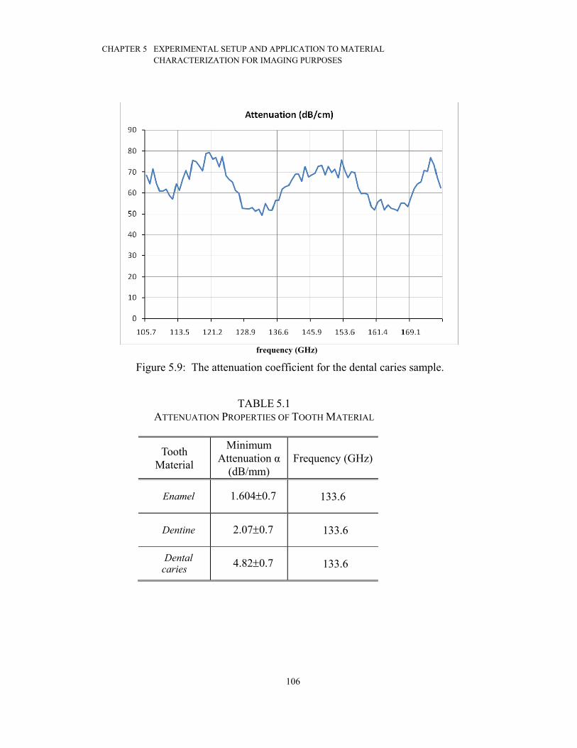
CHAPTER 5 EXPERIMENTAL SETUP AND APPLICATION TO MATERIAL CHARACTERIZATION FOR IMAGING PURPOSES
106
frequency (GHz)
Figure 5.9: The attenuation coefficient for the dental caries sample.
TABLE 5.1 ATTENUATION PROPERTIES OF TOOTH MATERIAL
Tooth Material
Minimum Attenuation α
(dB/mm) Frequency (GHz)
Enamel 1.604±0.7 133.6
Dentine 2.07±0.7 133.6
Dental caries 4.82±0.7 133.6

CHAPTER 5 EXPERIMENTAL SETUP AND APPLICATION TO MATERIAL CHARACTERIZATION FOR IMAGING PURPOSES
107
The main achievements of the spectroscopic measurements of tooth is that
it gives us an indication and values of refractive index and attenuation values for the various materials of tooth under study for imaging purposes. The changes in the refractive index of enamel, dentine, and dental caries as well as change in the attenuation coefficient in theses materials at the mm-Wave and THz range can be exploited for imaging of teeth.
The material properties of the tooth at 133.626 GHz is shown in Table 5.2 and can be used in the CAD model, where the region of the tooth that is above the gums is illuminated by a Gaussian beam and the field is measured everywhere. The modeling of the spherical lens and the tooth that includes the effect of the curvature and the multi-layer 3D structure using a commercial simulator and SRT will be considered in the future for the continuous-wave setup.
TABLE 5.2 ELECTRICAL PROPERTIES OF TOOTH AT THZ RANGE
Tooth Material
Refractive index n [76] rε Attenuation α
(dB/mm) tan δ
Enamel 3.06 9.364 1.604 0.937
Dentine 2.57 6.605 2.07 3.221

CHAPTER 5 EXPERIMENTAL SETUP AND APPLICATION TO MATERIAL CHARACTERIZATION FOR IMAGING PURPOSES
108
5.2 Terahertz Imaging Setup
For a coherent THz beam incident on the tooth sample, SRT is promising in modeling the local interaction of the THz beam with the tooth sample. In the transmission mode imaging, an image is formulated based on the transmitted beam after multiple reflections and refraction through the sample. At 1.2 THz range, with a wavelength of 250μm or less, the curvature matrices would work with some curvature of the tooth being more than 6 mm. Since the tooth is large compared to the wavelength, SRT is suitable for modeling THz propagation through it assumes the material properties of the enamel and dentine vary slowly over the wavelength. I would like to thank Dr. Daryoosh Saeedkia, Mohammad Neshat, and Bahar Davoudi, for the collaboration on the imaging setup and discussion.
The quality of a THz imaging system is determined by its diffraction limit, alignment and focus beam. Diffraction manifests itself in the bending of the beam around small obstacles, and the spreading out of the beams past small openings with dimensions comparable to the wavelength of the beam. In order to find the diffraction, the Fraunhofer diffraction equation for a circular aperture is used [80] due to the circular aperture employed in the experiment.
Where q = 2 2ξ η+ is the radius in the aperture plane and 2 2x yf fρ = + is the
radius in the spatial frequency domain. For the unit-amplitude plane wave
incidence on the aperture, the Bessel function 1(2 )J wqB circ Aw w
π ρπ ρ
⎧ ⎫⎛ ⎞ =⎨ ⎬⎜ ⎟⎝ ⎠⎩ ⎭
and
the intensity distribution has an Airy pattern[80]
Or2
10
( sin )( ) 2sin
J kaI Ika
θθθ
⎡ ⎤= ⎢ ⎥⎣ ⎦, where J1 is the Bessel function of the first kind of
order one and A = πw2, where w is the radius of the circular aperture. The radius of the main lobe of the Airy disk represents the limit of the resolution for the diffraction-limited system
2
2/( ) ( )
krjkz jz
r zeU r e B U qj z ρ λλ == . (5.3)
221( / )( ) 2
/J kwr zAI r
z kwr zλ⎡ ⎤⎛ ⎞= ⎜ ⎟ ⎢ ⎥⎝ ⎠ ⎣ ⎦
(5.4)
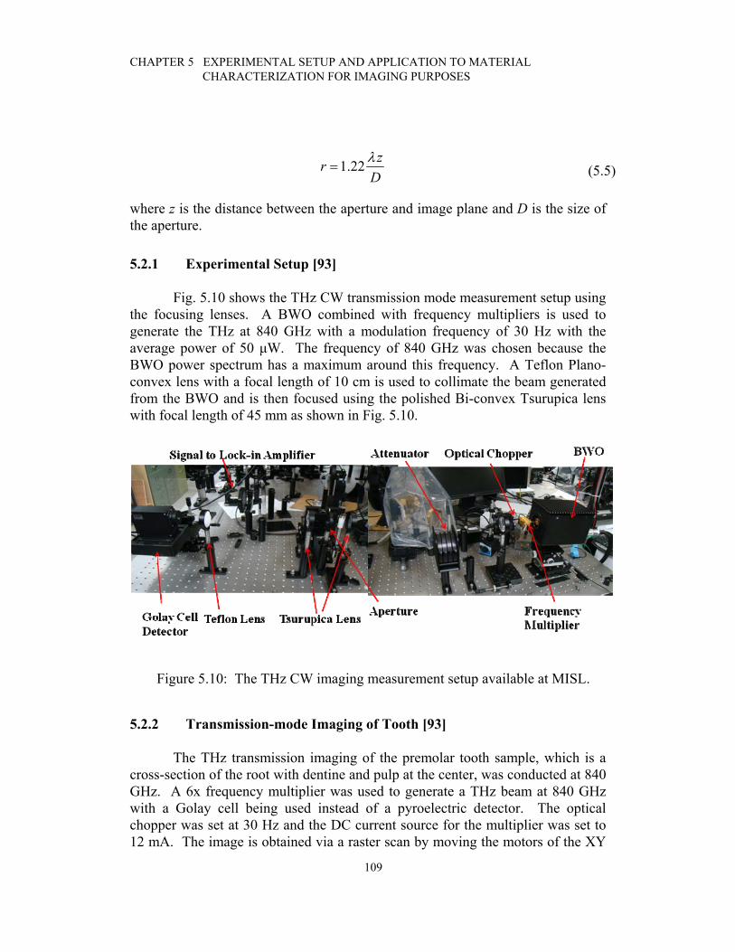
CHAPTER 5 EXPERIMENTAL SETUP AND APPLICATION TO MATERIAL CHARACTERIZATION FOR IMAGING PURPOSES
109
where z is the distance between the aperture and image plane and D is the size of the aperture.
5.2.1 Experimental Setup [93]
Fig. 5.10 shows the THz CW transmission mode measurement setup using the focusing lenses. A BWO combined with frequency multipliers is used to generate the THz at 840 GHz with a modulation frequency of 30 Hz with the average power of 50 μW. The frequency of 840 GHz was chosen because the BWO power spectrum has a maximum around this frequency. A Teflon Plano-convex lens with a focal length of 10 cm is used to collimate the beam generated from the BWO and is then focused using the polished Bi-convex Tsurupica lens with focal length of 45 mm as shown in Fig. 5.10.
Figure 5.10: The THz CW imaging measurement setup available at MISL.
5.2.2 Transmission-mode Imaging of Tooth [93]
The THz transmission imaging of the premolar tooth sample, which is a cross-section of the root with dentine and pulp at the center, was conducted at 840 GHz. A 6x frequency multiplier was used to generate a THz beam at 840 GHz with a Golay cell being used instead of a pyroelectric detector. The optical chopper was set at 30 Hz and the DC current source for the multiplier was set to 12 mA. The image is obtained via a raster scan by moving the motors of the XY
1.22 zrDλ
= (5.5)

CHAPTER 5 EXPERIMENTAL SETUP AND APPLICATION TO MATERIAL CHARACTERIZATION FOR IMAGING PURPOSES
110
stage using LabView and using Matlab to acquisition data from the Lock-in amplifier.
The corresponding measured point spread function is shown in Fig. 5.11.
The scan time was 2 minutes per line and the resolution was set to 0.25 mm. Fig. 5.12 shows the THz image alongside the visible image of the cross-section of the tooth. It shows that the Mylar wall and polyethylene holding the tooth slice has a high transmittance while the tooth dentine and pulp have high absorption.
0 1 2 3 4 5 6 7 8-1
0
1
2
3
4
5
6x 10⁻⁴
Sig
nal (
V )
mm Figure 5.11: The measured Point Spread Function along horizontal x-axis at 840 GHz.
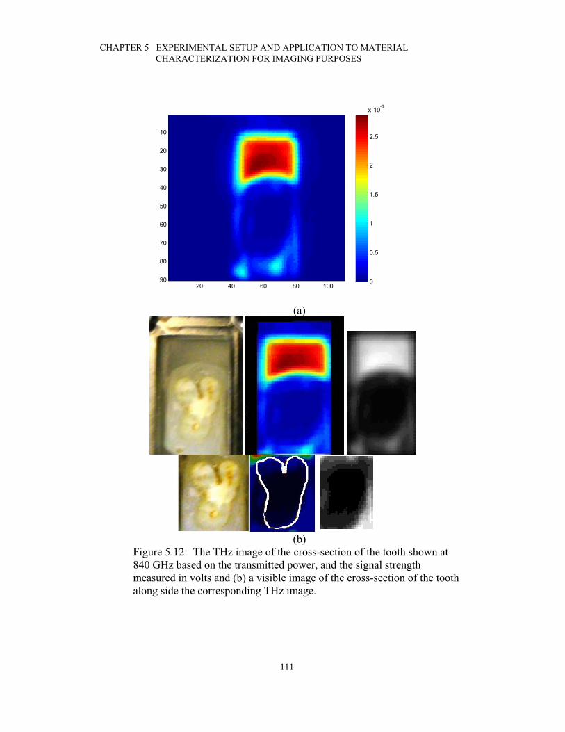
CHAPTER 5 EXPERIMENTAL SETUP AND APPLICATION TO MATERIAL CHARACTERIZATION FOR IMAGING PURPOSES
111
20 40 60 80 100
10
20
30
40
50
60
70
80
90 0
0.5
1
1.5
2
2.5
x 10-3
(a)
(b)
Figure 5.12: The THz image of the cross-section of the tooth shown at 840 GHz based on the transmitted power, and the signal strength measured in volts and (b) a visible image of the cross-section of the tooth along side the corresponding THz image.

CHAPTER 5 EXPERIMENTAL SETUP AND APPLICATION TO MATERIAL CHARACTERIZATION FOR IMAGING PURPOSES
112
5.2.3 The Beam Profile in a Continuous-wave Imaging Setup
We assume the THz beam generated by the BWO and propagating through the multiplier waveguide has the form of a Gaussian beam. First, a Gaussian beam profile without astigmatism is assumed to find the beam profile, and the lens is approximated as a thin lens without aberrations to calculate the beam waist. The beam profile is useful in enhancing the image resolution such as the one in Fig. 5.12. The focus beam for the CW imaging setup is then measured to find the beam profile and size. The Gaussian beam is a solution to the paraxial Helmholtz equation and the complex amplitude of the Gaussian beam traveling along the z-direction is given as [81]
Where 1
0( ) tan zz
zξ − ⎛ ⎞
= ⎜ ⎟⎝ ⎠
is the phase delay of the wavefront in comparison to a
plane wave or spherical wave, and
0z is the Rayleigh range, W0 is the waist radius and R(z) is the wavefront radius of the curvature. The Gaussian beam resembles a plane wave at the beam center and a spherical wave with a phase delay at large z. The Gaussian beam has its maximum curvature at 0z , where the beam radius is 2 times greater than the radius at the beam waist. The intensity on the beam axis is half its peak value and the phase is retarded by 45 degrees relative to the phase of a plane wave. The intensity is given by [81]
2 20
0 2( ) exp exp ( )( ) 2 ( )( )
WU A jkz jk j zW z R zW z
ρ ρ ξ⎡ ⎤ ⎡ ⎤
= − − − +⎢ ⎥ ⎢ ⎥⎣ ⎦ ⎣ ⎦
r (5.6)
1/ 22
00
( ) 1 zW z Wz
⎡ ⎤⎛ ⎞⎢ ⎥= + ⎜ ⎟⎢ ⎥⎝ ⎠⎣ ⎦
(5.7)
20( ) 1 zR z zz
⎡ ⎤⎛ ⎞= +⎢ ⎥⎜ ⎟⎝ ⎠⎢ ⎥⎣ ⎦
(5.8)
00
zW λπ
= (5.9)

CHAPTER 5 EXPERIMENTAL SETUP AND APPLICATION TO MATERIAL CHARACTERIZATION FOR IMAGING PURPOSES
113
And the beam intensity drops from a pick value on the beam axis to
20
( ,0) 1 0.1353II eρ
= ≈ at the beam waist 0Wρ = . Fig. 5.11 shows the
measurement of the intensity of the beam transmitted through a pinhole located at the focus of the beam ( ,0)I ρ which is plotted along the horizontal position at 840 GHz. The beam width is found experimentally by measuring the distance from the beam axis to where the value of the normalized intensity and is about 0.1353[81]. The beam waist was measured to be 1.77 mm at 840 GHz (see Fig. 5.11).
The beam waist is calculated based on the Gaussian beam assumption at the focus by using the principle of beam shaping using a lens. The BWO waveguide is placed at the focus of lens 2 in Fig. 5.2 and a collimated beam with a Rayleigh range of z1 propagates to the focusing lens 5. The resulting transmitted beam is focused with a smaller beam waist at distance z0 given by [81]
Where f is the focal length of the lens and W1 is half of the spot size of the incident collimated beam, and the spot size of the collimated beam 2W1 is at least equal to the diameter of the lens D. The focal length of the lens is f = 10 cm, and n = 1.52. It is found that 12 2.5 W cm= through the measurements by putting an aperture before lens 5 and finding the smallest size of the pinhole for which the detected signal would stay equal to its maximum value. Using Eq. (5.11), z1 is
found using W1 and Eq. (5.12) gives the beam waist 01
42 1.82 2
fW mmW
λπ
≅ = .
After a 2D raster-scan of the intensity of the focused beam is transmitted through the quasi-optical system, the intensity is measured and after deconvolution we obtain the beam profile. The maximum signal obtained without the sample before deconvolution is 3.324 mV corresponding to 1.375 μW at (5 mm, 5 mm) . Fig. 5.13(a) shows the intensity of the focused beam generated by BWO. The lens system followed by the deconvolved beam profile of the THz
2 20
0 22( , ) exp
( ) ( )WI z I
W z W zρρ
⎡ ⎤⎡ ⎤= −⎢ ⎥⎢ ⎥
⎣ ⎦ ⎣ ⎦. (5.10)
10 2
11 ( / )
WWz f
=+
(5.11)
0 211 ( / )
fzf z
=+
(5.12)
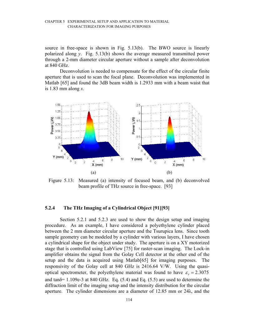
CHAPTER 5 EXPERIMENTAL SETUP AND APPLICATION TO MATERIAL CHARACTERIZATION FOR IMAGING PURPOSES
114
source in free-space is shown in Fig. 5.13(b). The BWO source is linearly polarized along y. Fig. 5.13(b) shows the average measured transmitted power through a 2-mm diameter circular aperture without a sample after deconvolution at 840 GHz.
Deconvolution is needed to compensate for the effect of the circular finite aperture that is used to scan the focal plane. Deconvolution was implemented in Matlab [65] and found the 3dB beam width is 1.2933 mm with a beam waist that is 1.83 mm along x.
(a) (b)
Figure 5.13: Measured (a) intensity of focused beam, and (b) deconvolved beam profile of THz source in free-space. [93]
5.2.4 The THz Imaging of a Cylindrical Object [91][93]
Section 5.2.1 and 5.2.3 are used to show the design setup and imaging procedure. As an example, I have considered a polyethylene cylinder placed between the 2 mm diameter circular aperture and the Tsurupica lens. Since tooth sample geometry can be modeled by a cylinder with various layers, I have chosen a cylindrical shape for the object under study. The aperture is on a XY motorized stage that is controlled using LabView [75] for raster-scan imaging. The Lock-in amplifier obtains the signal from the Golay Cell detector at the other end of the setup and the data is acquired using Matlab[65] for imaging purposes. The responsivity of the Golay cell at 840 GHz is 2416.64 V/W. Using the quasi-optical spectrometer, the polyethylene material was found to have 2.3075rε = and tanδ= 1.109e-3 at 840 GHz. Eq. (5.4) and Eq. (5.5) are used to determine the diffraction limit of the imaging setup and the intensity distribution for the circular aperture. The cylinder dimensions are a diameter of 12.85 mm or 24λ, and the

CHAPTER 5 EXPERIMENTAL SETUP AND APPLICATION TO MATERIAL CHARACTERIZATION FOR IMAGING PURPOSES
115
height is 20 mm and placed 20 mm from Lens 2. The effect of the cylinder is observed. The motor speed is 0.1 mm/s, that is determined by the resolution of 100 μm. After proper alignment, the scan time at a scanning frequency of 8 Hz took 1 min 41 sec. per line or a total time of 3 hours for an imaging area of 10 mm × 10 mm. The intensity passing through the lenses, sample and the aperture is measured using the Golay cell. The Lock-in amplifier has an auto-phase feature that calibrates the phase of the in-phase component of the measured signal with the signal coming from the optical chopper. The imaging process is performed by sampling the focal plane field. This is carried out by a pin hole. For a plane-wave incident on the aperture, the Fraunhofer diffraction equation is [80]
Where q is the radius in the aperture plane, J1 is of the first kind Bessel function with an order of one, and ρ is the radius in the spatial frequency domain. This is used to determine the simulated point spread function used for deconvolution. The intensity distribution for the circular aperture with a plane wave incidence is an Airy disk, where w is the radius of the circular aperture. The Airy disk pattern of the intensity is considered for plane-wave incident on the aperture. This is used in the deconvolution process.
The experimental setup for the THz propagation through a cylinder is
shown in Fig. 5.14. After a 2D raster scan, the maximum signal obtained after the transmission through cylindrical sample is 0.456 mV or 0.189 μW with a SNR of 17.6dB at the focal plane. The focal plane along z was adjusted to compensate for the change of the focused beam due to the cylinder. Fig. 5.15 shows the measured beam profile after the transmission through the cylindrical polyethylene sample with a 3dB beam width of 1.2125 mm or a beam waist of 1.725 mm along x. When compared to the case for free-space, the beam waist shrunk by 5.74% along x and expanded along y becoming more astigmatic. The power loss due to the circular aperture is 0.6867 μW, and the power loss due to scattering and losses after transmission through the cylinder was 1.1695 μW or ratio of 0.15.
212 (2 )( )
kjkz j rz J weU r A e
j z wπ ρ
λ π ρ= (5.13)

CHAPTER 5 EXPERIMENTAL SETUP AND APPLICATION TO MATERIAL CHARACTERIZATION FOR IMAGING PURPOSES
116
Figure 5.14: Experimental setup for THz Propagation through a cylinder.
Figure 5.15: Measured deconvolved beam profile with and without sample in μW.

CHAPTER 5 EXPERIMENTAL SETUP AND APPLICATION TO MATERIAL CHARACTERIZATION FOR IMAGING PURPOSES
117
The second experimental setup for the CW Imaging of the polyethylene
cylinder is shown in Fig. 5.16. The cylinder is put at a focal plane. The polyethylene cylinder height is 20 mm and diameter is D = 12.85 mm. The measured THz image of polyethylene cylinder at 840 GHz is shown in Fig. 5.17.
Figure 5.16: The THz CW imaging of Polyethylene cylinder.
Figure 5.17: The THz image of Polyethylene cylinder.

CHAPTER 5 EXPERIMENTAL SETUP AND APPLICATION TO MATERIAL CHARACTERIZATION FOR IMAGING PURPOSES
118
5.3 The Comparison of the Transmission Image of the Cylinder Using the HSRT and Transmission Line Matrix (TLM) Method [94]
In this section, we consider the problem of the THz propagation through
inhomogeneous cylindrical structures. The Transmission Line Matrix (TLM) [83]-[86] method is applied to the THz range to exploit its advantages in modeling inhomogeneous media, lossy media, nonlinear devices [87] and meta-materials. It has been implemented in 3D and 2D cases. In this section, the THz propagation through an infinitely long electrically large homogeneous isotropic cylinder is modeled employing 2D TLM and 2D SRT for THz applications. In addition, the effect of adding a hole in the cylindrical sample is examined.
For electrically large homogenous structures, 2D Spectral Ray Tracing (SRT) is applied by extending the 3D SRT formulated for this kind of 2D Gaussian-beam–cylinder scattering problem. The 2D SRT is advantageous since it is fast for electrically large structures and homogeneous regions. In addition, it can be incorporated in a hybrid approach with 2D TLM. The methods are then compared and verified using the Finite-Difference Time-Domain (FDTD) method.
5.3.1 The Two-Dimensional Transmission Line Matrix Method (2D TLM) The 2D TLM algorithm is applied for modeling the Terahertz (THz)
Gaussian beam propagation through a cylindrical structure. The TLM is a time-domain space-discretizing method in which the dynamics of the EM field is found by applying Huygens’ Principle [85].
The TLM is applied to model the THz TMz-mode propagation through a cylinder. The 2D TLM algorithm for the case of the TM-mode uses shunt nodes and involves a sequence of scattering and connection steps. For each node, the total node voltage is given as:
Where the incident sinusoid 1i
kV on line 1 and the source sinusoid ik sV at k-th time
step, are scattered according to,
( )1 2 3 4ˆ2 2
ˆˆ4
i i i i ik k k k k s s
k zs s
V V V V V YV
Y G
+ + + +=
+ + (5.14)
CHAPTER 5 EXPERIMENTAL SETUP AND APPLICATION TO MATERIAL CHARACTERIZATION FOR IMAGING PURPOSES
119
The admittance ˆˆ ˆ4 s sY Y G= + + and the normalized capacitive stub admittance is
given by ˆˆ 4( 1), 0s r sY Gε= − = . The loss is added in the TLM method by
introducing a lossy stub with 1ˆ
sTL
lGZσ−
− Δ= , where the characteristic impedance of
each link line is TLZ . Another advantage of TLM is that the scattering matrix is equal to its inverse, implying that time reversal and time reversal radar-based imaging algorithms can be achieved by only reversing the process without changing the algorithm [86]. The structure and computation region is shown in Figs. 5.18 and 5.19. A TEM absorbing boundary condition is used to truncate the solution space. The input signal or incident field is a Gaussian beam given by
In the space domain and modulated with exponential
In the time domain, the source is located at xi = x0 plane and 0ω λ= .
1 1
2 2
3 3
4 41
r i
k k
V VV VV VV V+
⎡ ⎤ ⎡ ⎤⎢ ⎥ ⎢ ⎥⎢ ⎥ ⎢ ⎥=⎢ ⎥ ⎢ ⎥⎢ ⎥ ⎢ ⎥⎣ ⎦ ⎣ ⎦
S (5.15)
ˆ ˆ2 2 2 2 2ˆ ˆ2 2 2 2 2
1 ˆ ˆ2 2 2 2 2ˆˆ ˆ2 2 2 2 2
ˆ ˆ2 2 2 2 2
s
s
s
s
s
Y Y
Y Y
Y YY
Y Y
Y Y
⎡ ⎤−⎢ ⎥
−⎢ ⎥⎢ ⎥= −⎢ ⎥⎢ ⎥−⎢ ⎥⎢ ⎥−⎣ ⎦
S (5.16)
2
202
0( , )yw
zE x y E e
⎛ ⎞⎜ ⎟−⎜ ⎟⎝ ⎠= (5.17)
( )( )( ) ( , ) exp 1 , 1, 2,...i z o if t E x y k dt kω= − − =i (5.18)

CHAPTER 5 EXPERIMENTAL SETUP AND APPLICATION TO MATERIAL CHARACTERIZATION FOR IMAGING PURPOSES
120
5.3.2 Numerical Examples of TLM and SRT Techniques
To verify the accuracy of the proposed method we start with the application of homogenous circular cylindrical geometry structures, as shown in Fig. 5.18.
The far-field interaction with an infinitely long inhomogeneous circular polyethylene cylinder that has a radius of 10λ and 2.3rε = , was evaluated using 2D TLM. The |Ez| total electric field is shown in Fig. 5.19. The simulation was for a Gaussian beam propagation through a lossless 2D cylinder with a beam width of 2λ or w0=λ. For comparison, the electric field for the TMz mode propagation at 860 GHz is simulated using 2D SRT, which is a fast asymptotic method. The 2D TLM and 2D FDTD[50] used for the 1500 points observations made a line of x = 14 mm as shown in Fig. 5.20. The amplitude matching for the various methods is important especially for SRT and FDTD methods as we can only obtain amplitude intensity information from our imaging setup. The phase information cannot be obtained using the Golay Cell. The source in this study is a Gaussian beam located at a plane 7 mm from the center of the cylinder. A Gaussian beam is incident on the x = 0.5 mm plane, 3.5 mm from the cylinder. It is polarized along the z direction as in Eq. (5.17), where 0 1 V/mE = , the beam waist of 0w λ= and ( , ) 0yE x y = .
The corresponding spectral distribution is given by:
The Gaussian source, Eq. (5.17) and Eq. (5.19) has beam width of 2λ or w0=λ. The cylinder is 10λ or with an approximate radius of 3.5 mm and the source is 3.5 mm from the cylinder.
2 20
0 0 0.5( , ) , ( , ) 02
yw k
z x y y x yE wE k k e E k k
π
−= = (5.19)

CHAPTER 5 EXPERIMENTAL SETUP AND APPLICATION TO MATERIAL CHARACTERIZATION FOR IMAGING PURPOSES
121
0 5 10 15
-6
-4
-2
0
2
4
6
X Span in mm
Y S
pan
in m
m
Figure 5.18: The geometry of cylindrical structure and SRT backward launched
rays that hit the cylinder in the xy-plane is shown. Here the x = 0 is source plane and x = 14 mm is the observation plane.
O

CHAPTER 5 EXPERIMENTAL SETUP AND APPLICATION TO MATERIAL CHARACTERIZATION FOR IMAGING PURPOSES
122
Figure 5.19: The |Ez| total electric field shown is obtained from the 2D TLM simulation for Gaussian beam propagation through a lossless
2D cylinder with a beam width of 2λ or w0=λ. The cylinder has R=3.5 mm ≈ 10λ and the source is 3.5 mm from the cylinder.

CHAPTER 5 EXPERIMENTAL SETUP AND APPLICATION TO MATERIAL CHARACTERIZATION FOR IMAGING PURPOSES
123
-8 -6 -4 -2 0 2 4 6 80
0.1
0.2
0.3
0.4
0.5
0.6
0.7
Y (mm)
|Ez| V
/m
2D SRT2D TLM2D FDTD
(a)
-4 -3 -2 -1 0 1 2 3 4-200
-150
-100
-50
0
50
100
150
200
250
Y (mm)
Pha
se E
z
2D SRT2D TLM2D FDTD
(b)
Figure 5.20: The (a) magnitude and (b) phase of Ez obtained from 2D SRT, 2D TLM and 2D FDTD simulations of Gaussian beam propagation through a 2D cylinder. The location of observation is 14 mm from the source.

CHAPTER 5 EXPERIMENTAL SETUP AND APPLICATION TO MATERIAL CHARACTERIZATION FOR IMAGING PURPOSES
124
For the TLM simulation of the cylinder with a hole, the maximum number of time steps is K = 5,000. An absorbing boundary condition applied to a computation region of a 860 × 860 cell, and dl = 17.4 μm, where the discretization is 20 cells/wavelength. The elementary time step is dt = 4.11×10⁻⁵ ns. It took 4 hours on a PC with an Intel Centrino Duo 2.4 GHz processor and 6 GB of RAM. The magnitude of the electric field for Gaussian beam propagation through a cylinder is shown in Fig. 5.21.
Figure 5.21: The magnitude of the total electric field Ez obtained after the 2D TLM simulation for the Gaussian beam propagation, w0=λ, through a 7 mm diameter cylinder with a circular hole diameter of 2 mm at the center.
Fig. 5.22 shows the E-field distribution for the Gaussian beam propagation
through a lossy cylindrical dielectric at 860 GHz. The TLM method is used for solving the direct problem in the inverse scattering problems. A problem of a cylinder with holes with different sizes was introduced. Fig. 5.23(a) shows the dielectric profile under study for THz imaging and Fig. 5.23(b) shows the magnitude of Ez obtained from the 2D TLM simulation.
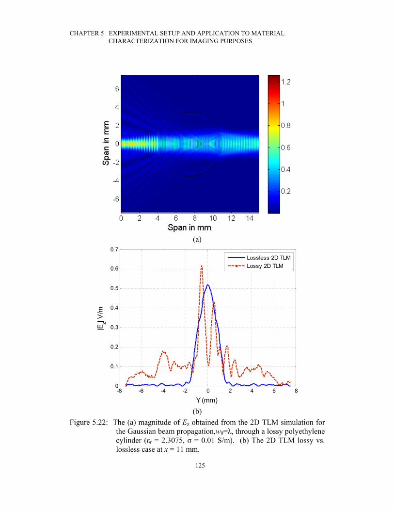
CHAPTER 5 EXPERIMENTAL SETUP AND APPLICATION TO MATERIAL CHARACTERIZATION FOR IMAGING PURPOSES
125
(a)
-8 -6 -4 -2 0 2 4 6 80
0.1
0.2
0.3
0.4
0.5
0.6
0.7
Y (mm)
|Ez| V
/m
Lossless 2D TLMLossy 2D TLM
(b)
Figure 5.22: The (a) magnitude of Ez obtained from the 2D TLM simulation for the Gaussian beam propagation,w0=λ, through a lossy polyethylene cylinder (εr = 2.3075, σ = 0.01 S/m). (b) The 2D TLM lossy vs. lossless case at x = 11 mm.

CHAPTER 5 EXPERIMENTAL SETUP AND APPLICATION TO MATERIAL CHARACTERIZATION FOR IMAGING PURPOSES
126
The 2D TLM and SRT codes were implemented using Matlab[65]. The time taken for the 2D SRT simulation was 7 minutes and 43 seconds with 210 backward rays launched, and 1500 observation points on the same PC with an Intel Centrino Duo 2.4 GHz processor and 6 GB of RAM. The TLM method took 10 hours for the resolution of 34.8 cells/wavelength, and 10,000 time steps. FDTD took 11 hours to simulate on the same PC. The discretization for FDTD was 34 samples per wavelength with the maximum number of time steps being 20,000. A PML absorbing boundary condition is applied around the computation region with 100 PML cells.
5.4 Conclusions In this chapter, a transmission-mode measurement for CW THz imaging
of polyethylene cylinder and cross-section of tooth is conducted using BWO. The beam profile of THz beam generated by a BWO was measured at the focal plane of a CW imaging system and the effect of electrically-large polyethylene cylinder on the beam profile examined. It was found that the focused beam becomes astigmatic and has more of an elliptical beam profile. THz transmission-mode CW imaging of a cross-section of premolar tooth sample with dentine and enamel was conducted at 840 GHz.
A two-dimensional Transmission Line Matrix (2D TLM) method is applied in the terahertz (THz) range to simulate wave propagation and scattering inside and around an inhomogeneous cylinder. The 2D TLM is applied for cylinders of 10λ in size giving accurate magnitude and phase results as compared to FDTD. The direct solution obtained using 2D TLM can be used for THz image reconstruction and hybrid 2D TLM and 2D SRT techniques for future study.

CHAPTER 5 EXPERIMENTAL SETUP AND APPLICATION TO MATERIAL CHARACTERIZATION FOR IMAGING PURPOSES
127
Span in mm
Spa
n in
mm
0 5 10 15
-6
-4
-2
0
2
4
6
1
1.2
1.4
1.6
1.8
2
2.2
(a)
(b)
Figure 5.23: The (a) dielectric profile of the structure to the image and (b) the magnitude of Ez obtained from the 2D TLM simulation for the Gaussian beam propagation, w0=λ, through a cylinder with a circular hole with diameter of 2.72 mm and elliptical hole with a diameter of 1.6 mm along x and 4.16 mm along y.

128
CHAPTER 6
Summary of Contributions and Future Work
6.1 Summary of Contributions
In this chapter the main contributions of our research and the major topics presented in this thesis are summarized. In this thesis, I have studied and investigated asymptotic methods for the computation of electrically large structures, Spectral Ray Tracing (SRT), terahertz integrated antennas, and biomedical applications of terahertz technology. SRT is an alternative for reliable computation of the electric field in the near-field and far-field without any approximation to solve an electrically large structure, while using less computational resources. A novel matrix representation of the SRT method is proposed, which requires only one spectral domain integration step for each observation point. SRT was compared with the rigorous Finite Element Method (FEM) and Geometrical Optics (GO) through the simulation of the terahertz Gaussian beam propagation through a hemispherical lens. The proposed method is also more accurate than Shooting and Bouncing Ray (SBR) method because SRT does approximation in the spectral domain and can include complex rays for near-field analysis. The GO response does not match SRT and HFSS responses because the lens surface is in the near-field of the source. SRT with a zero-order of reflection predicts the phase variation over angle θ much better than GO and the results are closer to the FEM simulations using Ansoft HFSS. The SRT method was able to accurately solve the problem 30 times faster than FEM. In addition it is effective in modeling quasi-optical systems including near-field analysis and promising for modeling the THz propagation through a biological media such as a tooth.
A rigorous computationally efficient self-consistent Hybrid SRT method is proposed to model complex multi-layer structures with sub-wavelength features, like an antenna close to large complex dielectric structures such as a lens or prisms. The Hybrid SRT (HSRT) is simple to implement and unlike the Uniform Theory of Diffraction (UTD), and the Uniform Asymptotic Theory (UAT) it can deal with the diffraction of an arbitrary wave, where the incident wave is decomposed into plane waves.

CHAPTER 6 SUMMARY OF CONTRIBUTIONS AND FUTURE WORK
129
The main contributions of this research have been:
• Reduction of SRT technique through novel matrix representation and comparison with FEM [88].
• A theoretical derivation of Spectral Ray Tracing from the Electromagnetics Reciprocity Theory [96].
• The proposed complexity reduced SRT was then combined with
MoM and FEM methods to constitute the new hybrid SRT algorithm, which enables the analysis of multi-scale millimeter-wave and terahertz integrated lens antennas [90][96].
• The extension of HSRT method to model lossy media to account for conductivity losses in lenses used in terahertz antennas. [96].
• The modeling of the THz receiver-transmitter link in free-space
using the SRT method and its linkage with the THz device models developed by other researchers in CIARS [92].
• As part of group work, an on-chip dipole integrated antenna with
VCO around 180 GHz was designed and characterized [97]. A new simple method to characterize the gain and radiation pattern of an embedded on-chip antenna is presented [97], where the feeding network is not accessible. This method only needs a sensitive power detector, and does not depend on expensive instrumentation such as wafer prober and network analyzer in the mmW/submmW range.
The HSRT algorithm was implemented in Matlab exploiting two GPUs for
parallel processing. The various versions of the Hybrid SRT method such as FEM-SRT, and MoM-SRT are compared and validated with commercial software Ansoft HFSS for the FEM method, FEKO for MoM, the Multi-level Fast Multipole Method (MLFMM) and Physical Optics (PO) via simulation of a bow-tie terahertz antenna backed by hyper-hemispherical silicon lens. The radiation patterns of an edge-coupled traveling-wave photomixer integrated with a bow-tie antenna, and a double-slot antenna backed by a hyper-hemispherical lens is obtained using MoM-SRT and FEM-SRT. It is shown that the MoM-SRT is more accurate than MoM-PO and comparable in speed.
The HSRT method is also applied to an on-chip Terahertz dipole antenna lens structure integrated with a VCO in SiGe:C BiCMOS technology backed by a silicon lens. The conductivity of the silicon lens was modeled by HSRT.

CHAPTER 6 SUMMARY OF CONTRIBUTIONS AND FUTURE WORK
130
The FEM-SRT method was able to accurately solve a double-slot antenna problem 77 times faster than FEM by exploiting parallel processing. The HSRT technique can be employed in an optimization loop to design antennas and other quasi-optical devices because it is computationally fast and accurate. Since the media of the systems modeled is linear, the solution and ray tubes obtained by SRT for a particular structure can be interpreted as the transfer function of the structure. The transfer function of the structure can then be re-used for the analysis of multi-antenna systems. In addition, it is shown that the matrix formulation of SRT and HSRT is a promising approach for parallel processing and solving complex electrically large problems with high accuracy. The use of GPU parallel processing greatly accelerates computational time of HSRT and SRT.
A transmission-mode measurement setup for the continuous wave and pulses THz imaging and spectroscopic imaging is developed in the Microwave and Terahertz Photonics Integrated Systems Lab (MISL). As an important application of interest in this lab, the dielectric characterization and spectroscopic measurements of different tooth samples, enamel, root dentine, and dental caries obtained from a dentist was conducted for the frequency range from 94.996 GHz to 176.282 GHz using a Backward Wave Oscillator (BWO). For the stated frequency range, 133.62576 GHz showed the least absorption by the enamel and dentine tissue samples. The measurements show that dental caries absorb more THz radiation than enamel but dentine has higher attenuation coefficient for frequencies between 141.27 GHz and 148.793 GHz than the dental caries. The average transmitted power was 41.5 mW for the enamel. The minimum attenuation was found to be 16.04±7 dB/cm for the enamel tissue at 133.62576 GHz, with a corresponding minimum attenuation of 20.67±7 dB/cm for the dentine, and 48.17±7 dB/cm for the dental caries. Near-field imaging at this frequency or using broadband signal centered at this frequency would enable the best penetration into the enamel tissue. The THz raster-scan imaging of a cross-section of tooth was also performed at 840 GHz. 6.2 Future Work
Accurate modeling of a THz transmitter-receiver link to model pulse propagation in free-space is important for modeling the emerging THz technologies in communications and imaging. This model includes The Tx, Rx antenna. The use of Hybrid SRT, by combining rigorous techniques to model a vertically-coupled traveling-wave photomixer integrated with a co-planar stripline and bow-tie antenna on LTG-GaAs, or a photoconductive dipole antenna on a GaAs substrate, as well as SRT for the analysis of the complex electrically large system including the hyper-hemispherical lens, and off-axis parabolic mirrors are

CHAPTER 6 SUMMARY OF CONTRIBUTIONS AND FUTURE WORK
131
important research tasks that need to be performed in the next stage. Once the the THz link measurement setup including the bow-tie antenna as a transmitter with the hyper-hemispherical lens, dipole antenna with the same lens as a transmitter, and the off-axis mirrors is complete, the measurements of the received pulse would be used to improve the HSRT model.
This research can be extended in many ways. Some of the proposed areas for future research are listed below:
• SRT is not easily applicable to resonance analysis as in [82].
Developing HSRT for dielectric resonators and electrically small lens with size of a wavelength or few wavelengths is important.
• Fully Coupling impressed source in rigorous numerical solver such as MoM with reflected wave coming from electrically large structure by solving MoM in presence of reflected field in addition to the impressed source (loading effects) will enhance the accuracy of the model.
• Thorough Ray Tracing modules are needed for tracing rays in irregularly shaped complex structures.
• SRT could be formulated and implemented to model the THz
propagation through biological samples such as homogeneous version of a tooth sample using electrical properties measured in Chapter 5, which is electrically large. It would be a forward model for the use in inverse-scattering problems and/or imaging with sub-wavelength resolution.

132
APPENDIX 1: Geometrical Optics
Geometrical optics (GO) is based on ray tracing methods. Ray methods deal with the evaluation of fields at high frequencies where parameters of the medium vary little over a wavelength. A ray is the idealization of a very narrow beam of light and is defined as the trajectory between a point of diffraction and the point of observation. In free space or in homogeneous regions, the rays are observed to be straight lines along which the light propagates. The propagation of geometrical optical rays is governed by Fermat’s principle, which states that the ray from point ro to point r is the curve C joining these two points for which optical distance 0( , )S r r or integral [27]
is minimum or the optical path, ds ndσ= , is stationary.
Figure A1.1: The geometrical optic ray from point r0 to point r is a curve C that
makes S(C), Eq. (A1.1), a minimum.
According to geometrical optics, the phase variation along a ray C propagating between two points is the product of the wave number k and distance between these two points, or 0 0( , )k S r r× is the phase of ray C from point r connected to the phase at point r0. 0 2 /k π λ= is the free-space wave number. When n(r) is a smooth function of r it can be shown that the condition Eq. (A1.1) implies that the ray C satisfies a differential equation. If n(r) is discontinuous, two rays are generated, one reflected and one refracted according to Snell’s law. For example, if k is the tangent vector of length onk at the point ( )r σ on C
determines the rate at which the tangent to C rotates or the curvature of C. Given the initial direction of the ray at point ro, the ray is found by integrating Eq. (A1.2).
( )C
S C ndσ= ∫ (A1.1)
0d k ndσ
= ∇k (A1.2)

133
Denoting 0( , )S r r by ( )S r , the phase 0 ( )k S r× must be continuous at the point of diffraction, except at the point of contact of the ray with its envelope, called a caustic. These usually occur at a focus, where an infinite number of rays converge to form an image, or on the caustic surfaces to which all rays are tangent. A caustic exhibits a jump discontinuity and the simple theory predicts an infinite amplitude [27][33].
One of the laws of geometrical optics is power conservation used to find the amplitude of the field once we find the system of rays throughout a system or phase of the field. Figure A1.2 shows the tube of rays close to a ray and intensity law[27][28][31]. The power carried by a tube of rays is proportional to the square of the field amplitude and is conserved along a tube of rays. The amplitude of the ray field is inversely proportional to the square root of the cross-sectional area of the tube of rays.
Figure A1.2: The tube of rays emanating from point r0. Intensity law: 1 1 2 2I d I d I dΩ∑ = ∑ = Ω , Courtesy of [27][62].
The Intensity Law
The intensity I, expressed by the energy crossing, per unit time, a unit surface element normal to the ray, is
where A is the field amplitude with a factor that depends on the quantity (E or H) used to describe the field, /v c n= is the velocity at which the energy in the field moves along the rays. In Fig. A1.2, the small cross sections of areas 1d ∑
2I A v= (A1.3)
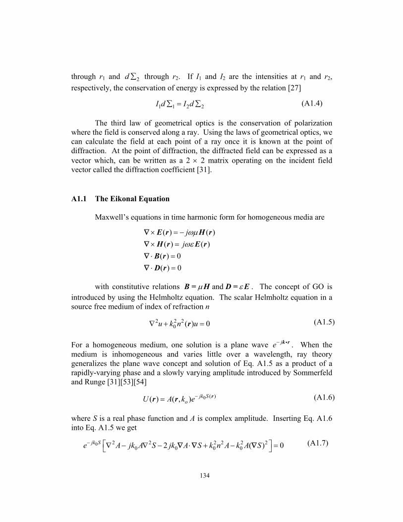
134
through r1 and 2d ∑ through r2. If I1 and I2 are the intensities at r1 and r2, respectively, the conservation of energy is expressed by the relation [27]
The third law of geometrical optics is the conservation of polarization where the field is conserved along a ray. Using the laws of geometrical optics, we can calculate the field at each point of a ray once it is known at the point of diffraction. At the point of diffraction, the diffracted field can be expressed as a vector which, can be written as a 2 × 2 matrix operating on the incident field vector called the diffraction coefficient [31].
A1.1 The Eikonal Equation
Maxwell’s equations in time harmonic form for homogeneous media are
with constitutive relations andμ εB = H D = E . The concept of GO is introduced by using the Helmholtz equation. The scalar Helmholtz equation in a source free medium of index of refraction n
For a homogeneous medium, one solution is a plane wave je− k ri . When the medium is inhomogeneous and varies little over a wavelength, ray theory generalizes the plane wave concept and solution of Eq. A1.5 as a product of a rapidly-varying phase and a slowly varying amplitude introduced by Sommerfeld and Runge [31][53][54]
where S is a real phase function and A is complex amplitude. Inserting Eq. A1.6 into Eq. A1.5 we get
1 1 2 2I d I d∑ = ∑ (A1.4)
( ) ( )( ) ( )
( ) 0( ) 0
jjωμωε
× = −× =⋅ =⋅ =
E r H rH r E r
B rD r
∇∇∇∇
2 2 20 ( ) 0u k n u∇ + =r (A1.5)
0 ( )( ) ( , ) jk SoU A k e−= rr r (A1.6)
0 2 2 2 2 2 20 0 0 02 ( ) 0jk Se A jk A S jk A S k n A k A S− ⎡ ⎤∇ − ∇ − ⋅ + − =⎣ ⎦∇ ∇ ∇ (A1.7)

135
using property 2 2 2( ) 2AB A B A B A∇ = ∇ + ⋅ Β+ ∇∇ ∇ . For 1/k being small or in the high frequency limit, 0k →∞ ,
Letting the coefficients of the various powers of k0 be zero in Eq. A1.8 results in the eikonal equation
where S is the eikonal or wavefront surface. And the transport equation for m= 0
And for m > 0
These equations contain all the laws of the geometrical optics for scalar waves. Using vector notation in free-space, the transport equation becomes
Since 0∇ =Ei and inserting in the Luneberg-Kline asymptotic expansion
we have for m = 0
From the transport equation, if A0 is a Cartesian component of u0, Eq. A1.10 becomes 2
0( ) 0A S∇⋅ ∇ = and the flux in a tube of rays is conserved, 2 2
0 0( ) ( ) (0) (0)z zΣ = Σu u . The transport equation is solved using the ray
coordinate system, where z is along the ray and 1X and 2X are the principle directions of the wavefront. The Laplacian in this coordinate system is
0 0 1 220 0
1 1( , ) ( ) ( ) ( ) ...A k A A Ajk k
= + − +r r r r (A1.8)
2 2S n∇ = (A1.9)
20 02 0A S A S∇ + ⋅ =∇ ∇ (A1.10)
2 212m m mA S A S A −∇ + ⋅ = ∇∇ ∇ . (A1.11)
20( 2 0S S∇ + ⋅ =u∇ ∇) . (A1.12)
( )
0( ) ( ) ( ) ( )
MjkS r m M
mm
r e jk r o k− − −
=
= +∑E u , (A1.13)
0 0S∇ ⋅ =u . (A1.14)

136
where 11
1 zhR
= + , 22
1 zhR
= + , and h =1, and R1 and R2 are the principal radii of
curvature along 1X and 2X . Since S is constant on a wavefront, 1 2
0,S Sx x∂ ∂
= =∂ ∂
so
Along a ray,
And the transport equation Eq. A1.10 becomes
Thus 0 1 2
0 1 2
( )(0) ( )( )
A z R RA R z R z
=+ +
and
Eq. A1.19 shows the divergence factor and the field amplitude is conserved in a tube of rays.
A1.2 Ray Tracing
The surfaces on which ( )S r is constant are called wave surfaces or wavefronts. Rays are the orthogonal trajectories of the wavefronts. At any point r, the vector of length 0 ( )k n r tangent to the ray is
2 1 2 2 1
1 2 1 1 1 2 2 2
1 h h h h h hS S SSh h h z h z x h x x h x
⎧ ⎫⎛ ⎞ ⎛ ⎞∂ ∂ ∂ ∂ ∂ ∂⎪ ⎪⎛ ⎞∇ = + +⎨ ⎬⎜ ⎟ ⎜ ⎟⎜ ⎟∂ ∂ ∂ ∂ ∂ ∂⎝ ⎠⎪ ⎪⎝ ⎠ ⎝ ⎠⎩ ⎭. (A1.15)
2
1 2
1 1SR z R z
∇ = ++ +
. (A1.16)
00 0
dAS A z Adz
∇ ⋅∇ = ⋅∇ = (A1.17)
00
1 2
1 12 0dA Adz R z R z
⎛ ⎞+ + =⎜ ⎟+ +⎝ ⎠
. (A1.18)
1 20 0
1 2( ) (0)
( )( )R Rz
R z R z=
+ +u u . (A1.19)
( ) 0 ( )r k S r= ∇k (A1.20)

137
As consequence of Eq. (A1.20),the rays are everywhere normal to the wavefront
[27]
Eq. A1.22 is the eikonal equation derived in Appendix A1.1. The phase varies as it would for a plane wave with wave vector k in the vicinity of r, thus the field is locally a plane wave. The rays that are near an axial ray are called paraxial and are said to form a pencil [31]. By finding the variation of the cross section of a Tube of Paraxial Rays (TPR) within the pencil, we can deduce the intensity variation of the field along the axial ray[27]. The rays of TPR are normal to family of wavefronts and in uniform regions, where all rays are straight lines. In the neighborhood of the axial ray Oz, we can represent the wavefront through point O by the second-degree equation [27]
where 1 2[ ]Tx x=x is the transverse position vector represented by its components (x1, x2) with respect to an orthonormal frame of reference, and Q is a 2 × 2 symmetric matrix called the curvature matrix [27][28]. Eq. A1.22 is an approximation to the wavefront. Fig. A1.3 shows the wavefront of the TPR. By
calculating the gradient of 12
T Q⋅z + x x , the vectors normal to wavefront are
obtained in the directions of propagation of paraxial rays. We obtain the normal vector ˆ Qz + x , where it is a unit vector along z direction and whose component transverse to the direction z is Qξ = x . The matrix Q has two orthogonal eigenvectors, 1 2 and X X , such that
for i = 1 and 2. In general, 1R and 2R are the principal radii of curvature, and the planes 1zX and 2zX are the principal planes. The rays of the TPR in the planes
0 ( )k n r=k (A1.21)
2 2( ) ( )S r n r∇ = (A1.22)
12
T Q= −z x x (A1.23)
1i i
iQ
RX = X (A1.24)
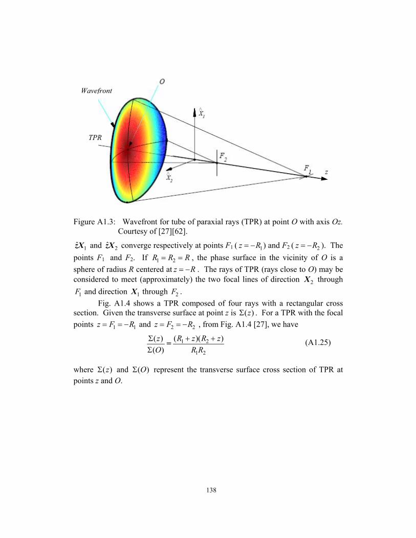
138
Figure A1.3: Wavefront for tube of paraxial rays (TPR) at point O with axis Oz.
Courtesy of [27][62].
1zX and 2zX converge respectively at points F1 ( 1z R= − ) and F2 ( 2z R= − ). The points F1 and F2. If 1 2R R R= = , the phase surface in the vicinity of O is a sphere of radius R centered at z R= − . The rays of TPR (rays close to O) may be considered to meet (approximately) the two focal lines of direction 2X through
1F and direction 1X through 2F . Fig. A1.4 shows a TPR composed of four rays with a rectangular cross
section. Given the transverse surface at point z is ( )zΣ . For a TPR with the focal points 1 1z F R= = − and 2 2z F R= = − , from Fig. A1.4 [27], we have
where ( )zΣ and ( )OΣ represent the transverse surface cross section of TPR at points z and O.
1 2
1 2
( )( )( )( )
R z R zzO R R
+ +ΣΣ
= (A1.25)
Wavefront
TPR
z

139
Figure A1.4: A TPR with the variation of the cross section, courtesy of [27][62].
The focal points of TPR are the caustic points. The intensity varies as
and the amplitude is proportional to the square root of the intensity. The ratio Eq. A1.25 may be negative and as consequence the amplitude will sometimes be imaginary. The reason is that the phase changes by 2
π of the TPR crossing a focal line. At point z, the curvature matrix Q, referred to the principal axes 1X and 2X is
Therefore, the variation of Q with z can be represented by
( )( )
z
O
I OI z
Σ=Σ
(A1.26)
1
2
1 0
10
R zQ
R z
⎡ ⎤⎢ ⎥+⎢ ⎥=⎢ ⎥⎢ ⎥+⎣ ⎦
. (A1.27)
1 1 1 0( ) ( )
0 1Q z Q O z− − ⎡ ⎤
= + ⎢ ⎥⎣ ⎦
(A1.28)
TPR
z

140
holds in any system of axes, orthogonal or not. From Eq. A1.25 and Eq. A1.27, we obtain
For a TPR, since the paraxial rays are almost parallel to the axis Oz, the phase of the field at point x in the plane z =0 is obtained by adding the phase at point O and 1
2Tk Q⋅x x neglecting higher order terms. The phase at any point
( , )r z= x when x is small is ( )kS r with
and Q(z) given by Eq. A1.28. The intensity and phase, Eq. A1.29 and A1.30, of the field propagating in a TPR, where 1 2det( ( )) 1/Q O R R= , is then
In Eq. A1.31, we suppose ( )Ou and ( )Q O are known and calculate Q(z) using Eq. A1.28 and S(r) using Eq. A1.30. For our application ( )ru is the electric field E . The second term of Eq. A1.31 is the factor of divergence DF after using Eq. A1.28 it becomes
A1.3 Refraction At A Curved Dielectric Interface [27][28][34]
Figure A1.5 presents an incident TPR, the surface,Σ ,the reflected and refracted TPR. First we examine the TPR refraction and consider TPR reflection as a special case of refraction. We utilize a principle of phase matching which is a direct consequence of Snell-Descartes’ law states the phase of the refracted TPR at every point of the surface Σ is the same as that in the incident TPR. Let the axis ˆiOz of the axial ray of the incident TPR, TPRi , and n the normal vector to the surface at point O. The angle 1α is the angle between them ( n and ˆiOz ). We are then able to model approximately the surface Σ around O using the equation
( ) det( ( )) ( ) det( ( ))z Q z O Q OΣ × = Σ × . (A1.29)
1( ) ( )2
TS r z Q z= + ⋅x x (A1.30)
12
( )det( ( ))( ) ( )det( ( ))
jkS rQ zr O eQ O
−⎡ ⎤= ⎢ ⎥
⎣ ⎦u u .
(A1.31)
1 2
1 1( )1 1
DF zz zR R
= ×+ +
. (A1.32)

141
where O=r r is the vector which is linked to point O at point r on the surface. If 1 2ˆ ˆ,u u represent orthonormal vectors, 1 1 2 2ˆ ˆt t= +t u u is the projection of r unto the
plane L tangent Σ at origin O. QΣ is the curvature matrix of Σ at point O. The phase of the incident TPR is ( )ik S r× where
The curvature matrix ( )i iQ z depends on iz but here we suppose that ( ) ( )i i iQ O Q z for iz in the neighborhood of O.
Figure A1.5: A TPR with wavefront curvature Qi refracted at a curved surface Σ . The reflected and refracted TPR have associated wavefront curvature matrices Qr and QR, courtesy of [62].
We express the vector ( )r t on the surface Σ , and inside the coordinate ( , )izx of incident TPR as follows
( )1 ˆ( )2
T QΣ= −r t t t t n (A1.33)
1( ) ( )2
Ti iS z Q O= +r x x (A1.34)
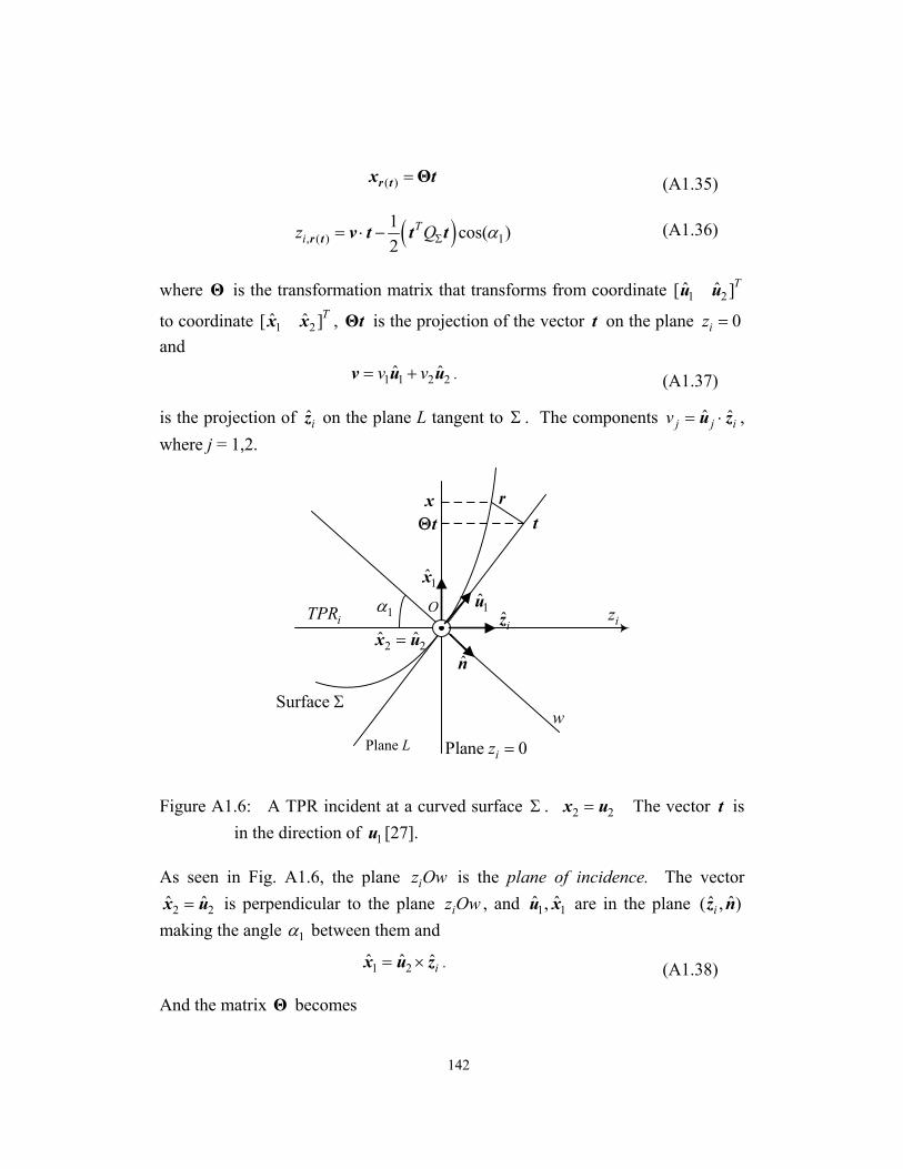
142
where Θ is the transformation matrix that transforms from coordinate 1 2ˆ ˆ[ ]Tu u
to coordinate 1 2ˆ ˆ[ ]Tx x , Θt is the projection of the vector t on the plane 0iz = and
is the projection of ˆiz on the plane L tangent to Σ . The components ˆ ˆj j iv = ⋅u z , where j = 1,2.
Plane L
O
Surface Σ
iTPR 1α
Plane 0iz =
1x
tΘx r
t
1uˆiz
n
iz
w
2 2ˆ ˆ=x u
Figure A1.6: A TPR incident at a curved surface Σ . 2 2=x u The vector t is in the direction of 1u [27].
As seen in Fig. A1.6, the plane iz Ow is the plane of incidence. The vector
2 2ˆ ˆ=x u is perpendicular to the plane iz Ow , and 1 1ˆ ˆ,u x are in the plane ˆˆ( , )iz n making the angle 1α between them and
And the matrix Θ becomes
( ) =Θr tx t (A1.35)
( ), ( ) 11 cos( )2
Tiz Q αΣ= ⋅ −r t v t t t (A1.36)
1 1 2 2ˆ ˆv v= +v u u . (A1.37)
1 2ˆ ˆ ˆi= ×x u z . (A1.38)

143
In general Θ is given by
And Substituting Eq. A1.36 into Eq. A1.34 for S(r ) we obtain
where
Eq. A1.41 is very important to determine the phase ( )ik S r× of the TPR incident on the surface Σ . The phase constitutes two terms, the linear term is Lk ⋅ = ⋅v t k t where Lk is the projection of the axial wave vector ˆo ik z vector on the tangent plane L, and the second term is quadratic defined by 2 2× symmetric matrix Γ .
The phase of the refracted TPR in passing through the surface Σ is represented by ( )R Rk S r× and
where
and RQ is the curvature matrix of the refracted TPR and RΘ is the same as Eq. A1.39 but with 1α replaced with 2α . In general, it is obtained by Eq. A1.40, where 1 2ˆ ˆ( , )x x is replaced by ,1 ,2ˆ ˆ( , )R Rx x that is a coordinate in the plane normal to ˆRz . ˆRz is the unit vector in the direction of the refracted TPR.
The principle of phase matching is applied to both the linear and quadratic terms at every point of Σ and so the phases of the incident TPR and refracted TPR coincide. We can write
1cos( ) 00 1α⎡ ⎤
= ⎢ ⎥⎣ ⎦
Θ . (A1.39)
1 1 1 2
2 1 2 2
ˆ ˆ ˆ ˆˆ ˆ ˆ ˆ⋅ ⋅⎡ ⎤
= ⎢ ⎥⋅ ⋅⎣ ⎦
x u x ux u x u
Θ . (A1.40)
( )1( )2
TS = ⋅ + Γr v t t t (A1.41)
1cos( )TQ Q αΣΓ = −Θ Θ . (A1.42)
1( )2
TR R RS = ⋅ + Γr v t t t (A1.43)
2cos( )TR R R RQ Q αΣΓ = −Θ Θ (A1.44)
R L=k k (A1.45)
R Rk kΓ = Γ (A1.46)

144
The condition Eq. A1.45 is Snell’s law applied to the axial ray
where n2 and n1 represent the indices of refraction for the second and first medium. The second Eq. A1.46 indicates the transformation of the curvature
Eq. A1.48 is important because it permits us to calculate the wavefront of the refracted TPR, in presence of the wavefront of incident TPR and of the matrix of curvature of the surface.
The wavefront of the reflected TPR is obtained using Eq. A1.51, setting Rk k= , and replacing 2α by 1π α− and
where rQ is the matrix of curvature of reflected TPR. Eq. A1.48 and Eq. A1.49 give us the matrices of curvature RQ and rQ at the points
Once RQ and rQ are determined from Eq. A1.48 and Eq. A1.49, the eigenvectors or principal directions of the wavefront, and their eigenvalues or principal curvatures can be found [28][33] The radius of curvature of refracted TPR and reflected TPR are the solutions of the quadratic equations given by
In order to find the factors of divergence of the refracted and reflected rays we use Eq. A1.32 and replace 1 2and R R by the radius of curvatures
1, 2, 1, 2,, and ,R R r rR R R R . If one knows the wavefront TPR, Tube of Paraxial Rays, incident on a
surface dielectric together with angle of incidence 1α as seen in Fig. A1.5, one can find the wavefronts of the reflected and refracted TPR by the following steps:
2 2 1 1sin( ) sin( )n nα α= (A1.47)
2 1( cos( ) cos( ))T TR R R R i Rk Q k Q k k Qα α Σ= + −Θ Θ Θ Θ (A1.48)
12cos( )T Tr r r iQ Q Qα Σ= −Θ Θ Θ Θ (A1.49)
( )( )
1, 2, 1, 2 2, 2
1, 2, 1, 2 2, 2
ˆ ˆ ˆ ˆ ˆ ˆˆ, and
ˆ ˆ ˆ ˆ ˆ ˆˆ, and
R R R R R R
r r r r r r
Q
Q
→ = × =
→ = × =
x x x u z x u
x x x u z x u
(A1.50)
1, 2, 21 1, : - ( ( )) det( ) 0 R R R RR R trace Q Q
RR+ = (A1.51)
1, 2, 21 1, : - ( ( )) det( ) 0 r r r rR R trace Q Q
RR+ = (A1.52)

145
Step 1 Get the directions of reflected and refracted TPR by using Snell’s Law (applied to the axial ray of the incident TPR).
Step 2 Get the plane of incidence ziOw plane, (see Fig. A1.6), and specify
the orthonormal vectors ( 1 2ˆ ˆ,u u ) from the tangent plane L such that
1u is in the plane of incidence and 2 1ˆ ˆ ˆu n u= × . Step 3 The matrix of curvature of the wavefront of the incident TPR iQ is
found given the vector 1 2( , )x x using Eq. A1.23 and Eq. A1.24, and calculate Θ using Eq. A1.40. When choosing
2 2 1 2ˆ ˆ ˆ ˆ ˆ and ix u x u z= = × and use Eq. A1.39. Step 4 Calculate Q∑ using Appendix A1.4. For spherical and cylindrical
surfaces we have
where
Step 5 Calculate RΘ using
where 2 2 1 1sin( ) sin( )n nα α= . Step 6 Calculate rΘ using
,
1 0
10sph
RQ
R
∑
⎡ ⎤⎢ ⎥
= ⎢ ⎥⎢ ⎥⎢ ⎥⎣ ⎦
(A1.53)
, ln
1 0
0 0cyQ R∑
⎡ ⎤⎢ ⎥=⎢ ⎥⎣ ⎦
(A1.54)
1 2ln
1 2
ˆ ˆ ˆ ˆˆ ˆˆ ˆcy
u u u uz u z uφ φ⋅ ⋅⎡ ⎤
= ⎢ ⎥⋅ ⋅⎣ ⎦A (A1.55)
2cos( ) 00 1Rα⎡ ⎤
= ⎢ ⎥⎣ ⎦
Θ (A1.56)

146
Step 7 Calculate rQ using Eq. A1.49 and RQ using Eq. A1.48. Step 8 Calculate the radius of curvature of the refracted TPR using Eq.
A1.51 and reflected TPR using Eq. A1.52. Step 9 Calculate RDF and rDF using Eq. A1.32. Step 10 Utilize the following equations to calculate the electric field at the
observation point:
where and T R are Fresnel coefficients of parallel and perpendicular polarization as in Appendix 1, b and c are the distances from the observation point to point O over the surface for the case of refraction and reflection, respectively. And ( )i Ou is the incident field at point O.
A1.4 Calculation of Matrix of Curvature for the Surface [28] At point of incidence O on surface, the following two vectors are in the
plane L of Fig. A1.6
where ˆ ˆ ˆ( , , ) x y z are evaluated at reference point. The matrix of curvature QΣ is given in terms of the base vectors 1 1( , ) x yr r by [28][33]
where
1cos( ) 00 1rπ α−⎡ ⎤
= ⎢ ⎥⎣ ⎦
Θ . (A1.57)
ˆ( ) ( ) ( )
ˆ( ) ( ) ( )
Rjk bR R R i
jkcr r r i
bz DF b T e O
cz DF c R e O
−
−
= × × ×
= × × ×
u u
u u.
(A1.58)
1
1
ˆ ˆˆ ˆ
x x
y y
x f zy f z
= +
= +
rr
(A1.59)
1 1 1 1 1 1 1 12
1 1 1 1 1 1 1 1
1 e G f F f E e FQ
f G g F g E f FΣ− −⎡ ⎤
= ⎢ ⎥− −Δ ⎣ ⎦ (A1.60)

147
and the vector normal n is
In the equations, ( )respectively x yf f is the partial derivative of ( , )f x y relative
to ,xx yyf f and xyf are the second-order derivatives of ( , )f x y , where ( , )z f x y= defines the surface Σ . The matrix of curvature QΣ expressed with
respect to 1 2ˆ ˆ( , )u u is
where
( )1
2 2 21 x yf fΔ = + + +
21 1 xE f= +
1 x yF f f=
21 1 yG f= +
11
11
11
xx
xy
yy
e f
f f
g f
−
−
−
= −Δ
= −Δ
= −Δ
( )1ˆ ˆ ˆ ˆx yn f x f y z= − − +Δ
(A1.61)
1Q A Q A−Σ Σ= (A1.62)
1 1 1 2
1 1 1 2
ˆ ˆˆ ˆ
x x
y y
u uA
u u⋅ ⋅⎡ ⎤
= ⎢ ⎥⋅ ⋅⎣ ⎦
r rr r
. (A1.63)
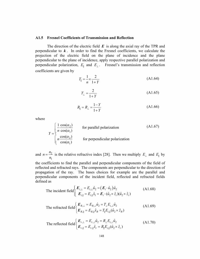
148
A1.5 Fresnel Coefficients of Transmission and Reflection
The direction of the electric field E is along the axial ray of the TPR and perpendicular to k . In order to find the Fresnel coefficients, we calculate the projection of the electric field on the plane of incidence and the plane perpendicular to the plane of incidence, apply respective parallel polarization and perpendicular polarization, E and E⊥ . Fresnel’s transmission and reflection coefficients are given by
where
and 2
1
nnn
= is the relative refractive index [28]. Then we multiply E⊥ and E by
the coefficients to find the parallel and perpendicular components of the field of reflected and refracted rays. The components are perpendicular to the direction of propagation of the ray. The bases choices for example are the parallel and perpendicular components of the incident field, reflected and refracted fields defined as
1 21
Tn Y
= ×+
(A1.64)
21
TY⊥ =
+ (A1.65)
11
YR RY⊥
−= =
+ (A1.66)
2
1
2
1
cos( )1 for parallel polarization cos( )cos( ) for perpendicular polarizationcos( )
nY
n
αααα
⎧⎪⎪= ⎨⎪⎪⎩
(A1.67)
( ), , 2 2 2
, , 1 2 2
ˆ ˆ ˆ The incident field
ˆ ˆ ˆˆ ˆ( )( )i i i
i i i i i
E u u uE x u z u z
⊥ ⊥⎧ = = ⋅⎪⎨ = = ⋅ × ×⎪⎩
E EE E
(A1.68)
, , 2 , 2
, , , 2
ˆ ˆ The refracted field ˆ ˆ ˆ( )
R R i
R R R i R
E u T E uE x T E u z
⊥ ⊥ ⊥ ⊥= =⎧⎨ = = ×⎩
EE
(A1.69)
, , 2 , 2
, , , 2
ˆ ˆ The reflected field ˆ ˆ ˆ( )
r r i
r r r i r
E u R E uE x R E u z
⊥ ⊥ ⊥ ⊥= =⎧⎨ = = ×⎩
EE
(A1.70)

149
A1.6 Discussion of Advantages and Disadvantages
Geometrical optics (GO) was an asymptotic method established long before the advent of Maxwell`s equations based upon the intuitive notion of rays that obey the laws of reflection and refraction in accordance with Fermat`s principle. Similar to PO, it is effective in modeling electrically large structures for far-field calculations at high frequencies. The disadvantages of GO is that, in contradiction to experimental observations, it predicts vanishing fields in the geometrical shadow regions. The theory of GO is for instance unable to reproduce the interference fringes of Young`s double slit experiment.
The GO ray-tracing method is enhanced by uniform asymptotic diffraction theories such as the Geometrical Theory of Diffraction (GTD), Uniform Asymptotic Theory (UAT), Uniform Theory of Diffraction (UTD). GTD was introduced to overcome the shortcoming of GO. It added the contribution of diffracted rays, especially those diffracted by the edges, that penetrate in the shadow zone. In common with GO, the phase varies linearly along a ray in GTD and power in a tube of rays is conserved. Employing the postulate that the diffracted field carried by a ray depends only on the local properties of the incident field and that of the object where it intercepts the ray, we can calculate each contribution to the diffraction by replacing the original scatterer with a canonical object for which the solution of the diffraction problem is known or can be easily solved [31]. The application of GTD is straightforward once the diffraction coefficient, which is defined as the ratio of the diffracted and incident ray fields, is found. So in practice, it is only necessary to identify the rays that are major contributors to the diffracted field and evaluate the field along each ray using GTD diffraction coefficients.

150
APPENDIX 2: Physical Optics
The scattering of E and H by a convex perfectly conducting scatter is
formulated as shown in Fig. A2.1 [53]. The scatterer is of simple shape with distinguished illuminated and shadow zones. The physical optics (PO) approximation considers the scatterer to be large electrically and the current density on the illuminated side is given by
and zero on the shadow side.
Figure A2.1: The physical equivalent for scattering from perfect electric conductor (PEC) with light-shadow boundary.
Using the current density Eq. A2.1, the vector potential is given as
In the far-zone,
In the direction of u and the scattered field is
where
ˆ2 iS n= ×HJ (A2.1)
1
'ˆ '
2 '
jksc i
S
e dsμπ
− −
= ×−∫ ∫
r r
nr r
A H (A2.2)
1ˆlim ' ( )
2 4
jkR jkRsc i jk
SR
e ee dsR R
μπ π
− −′⋅
→∞= × ⋅ =∫ ∫ n N uu rA H
(A2.3)
[ ( )]4
jkRsc sc ej j
Rω ω
π
−
= − = × × NE A u u u (A2.4)
S1 Sshadow
n
ˆ2 iS n= ×HJ
s sHE ,

151
The PO approximation shortcomings include that the transition from light to shadow is abrupt, while it should be continuous and that the curvature of the surface is neglected. The method fails in the presence of edges and vertices so physical theory of diffraction (PTD) was introduced to amend shortcomings [53].
A2.1 Application to Integrated Lens Antennas
Rutledge et al. [52] pioneered the use of substrate lens coupled to a planar antenna. Integrated antennas placed on dielectric lens with the same dielectric constant as the planar antenna substrate avoid power loss due to substrate modes. Dielectric lens come in various shapes such as hemispherical, hyper-hemispherical and ellipsoidal and adopted for millimeter-wave and terahertz applications from optics [52]. At terahertz frequencies, hyper-hemispherical silicon lens antennas are used to couple the terahertz radiation from photoconductive antennas to free space.
Filipovic et al. [30] and [55]-[59] applied geometrical optics/physical optics (GO/PO) methods to lens antenna design. In [30], the radiation patterns of a double-slot antenna on a silicon dielectric lens are computed using GO ray-tracing inside the dielectric lens and PO electric and magnetic field integration on the spherical dielectric surface. The analysis is applicable to planar antenna designed on dielectric lens and first decomposes the fields for a given ray into parallel/perpendicular components at the lens-air interface.
L
Silicon Wafers
Feed Antenna
Extension Length
R
Aperture Plane
r
r’
n
φ
incθ
Integration Plane Figure A2.2: The extended hemispherical lens used for the
geometric optics/physical optics technique [30].
1( ) 'jk
SSe ds′⋅= ⋅∫ ∫N J u ru (A2.5)

152
The equivalent electric and magnetic current densities [55] are calculated just outside the spherical surface using the GO electric field and magnetic fields
ˆs n= ×J H and ˆs n= ×M E , where n is the normal to the interface. The far-field transverse electric field is equal to
where N and L are defined as
where s′ is the closed surface just outside the lens, r′ is the distance from the origin of the coordinate system to the equivalent electric and magnetic currents, r is the distance from the origin to the far-field point, and ψ is the angle between r and r′ as in Fig. A2.2.
( )4
jkrjkerθ φ θη
π
−
≅ − +E L N (A2.6)
( )4
jkrjkerφ θ φη
π
−
≅ + −E L N (A2.7)
cosjkrSse dsψ′+ ′= ∫ ∫N J (A2.8)
cosjkrSse dsψ′+ ′= ∫ ∫L M (A2.9)

153
APPENDIX 3: Spectral Ray Tracing
A3.1 Physical Optics and Backward Ray Launching
The first step in Spectral Ray Tracing (SRT) consists of plane wave expansion of known source distribution in free-space. The SRT solution for free-space case is derived from electromagnetics reciprocity theorem and is given by
In step 2, the free space rays travel through various interfaces, where they experience reflection, refraction and diffraction[27][28]. The contribution of each individual plane wave in Eq. (A3.1) to total field at observation point is found by physical optics (PO) and stationary phase method (SPM). Fig. A3.1 The plane wave incident on interface S1.
02
0 ,( , ) 0
(1) 10 4
2
ˆˆ ˆ( ) ( , )
sin
x
y z m n
jm k xt x y
m n
jn k y jk zn n m
n E m k n k e
e k
πρ φ
θ θ φ
− Δ
− Δ −
≈ × Δ Δ
⋅ ⋅ Δ Δ
∑∑E r i
(A3.1)
z
x
0r
1ε
sr0 ˆiinc jE e x−= k rE i
1S
POM
POJ2ε
0 sr r−

154
Let us consider one particular plane wave impinging upon an interface S1. The PO sources, due to this incident wave, are placed on this interface generating the transmitted and reflected waves.
where 0 2 0 1ˆ and = .s s sR ψ ε ε= − − + kir r r r r Substituting the phase term
into fast-varying part of the integral in Eq. A2.2 we get
SPM is applied to PO integral to find the contribution of the aforementioned incident plane wave at the observation point.
where 1 2
0,x xψ ψ∂ ∂
= =∂ ∂
and H is the Hessian of ψ . After inserting the expansion
Eq. A3.4 into Eq. A3.3 we obtain [27] [31]
The amplitude 0
( )4
POs
sπ −J r
r r is slowly varying and the SPM expression is in the
form of ray tube with a ray path identical to what is predicted by GO and Snell’s law and divergence factor including radii of curvature of the transmitted QR / reflected Qr ray phasefront. The total field Eq. A3.1 at the observation point is therefore expressed below:
2 0
1
2 0
1
(1)0 1
1
( )4
4
i
i
i
j k R jPO
S
j k R jPO
S
ej dsR
e dsR
ε
ε
ωμπ
π
− − ⋅
− − ⋅
≈ −
−∇×
∫∫
∫∫
kE rk r
k r
J
M
(A3.2)
0
1
14
jkPO
S
e dsR
ψ
π
−
∫∫ J (A3.3)
12( ) ( ) ( )T
s s sψ ψ= + − −Hr u u u u (A3.4)
000
1
( ) ( )( ) 21
0
( )4 4
Ts ss
kPOjk jjkPO s
sS
e ds e e dR
ψψ
π π
+∞− − − −−
−∞−∫∫ ∫u u u urJ r
J ur r
H
(A3.5)
00 2 0 0 1
1
ˆ1
0 0
( ) 2 14 4 det ( )
s sPOjk
jk jkPO s
sS s
e ds eR k
ψε ε π
π π
−− − −≈
−∫∫ r r rJ rJ
r r rik
H (A3.6)

155
where ( , )m nT is the Fresnel transmission coefficient and l = 0 s−r r is the ray path length for each ray tube interacting with interface.
A3.2 The Transverse Vectors that Sample the PWS [62] Four vectors 1,( , ) 2,( , ) 3,( , ) 4,( , ), , and m n m n m n m nk k k k which surround the vector
,m nk . The directions of these vectors are
and ,m nk is from Eq. 2.12.
2
0 ,( , ) 00
10 ( , ) ( , )4
2,( , )
( ) ( , ) ( )
y z m nx
x x x y m n m nm n
jn k y jk zjm k xt m n
E E m k n k T DF l
e
π
− Δ −− Δ
Δ Δ
⋅ ⋅Δ
∑∑r
k
i
(A3.7)
1,( , ) ˆcos sin ,2 2
ˆ ˆ sin sin , cos2 2 2
m nm n m n
m n nm n n
d dk x
d d dk y k z
φ θφ θ
φ θ θφ θ θ
⎛ ⎛ ⎞ ⎛ ⎞= − −⎜ ⎜ ⎟ ⎜ ⎟⎝ ⎠ ⎝ ⎠⎝
⎞⎛ ⎞ ⎛ ⎞ ⎛ ⎞− − − ⎟⎜ ⎟ ⎜ ⎟ ⎜ ⎟⎝ ⎠ ⎝ ⎠ ⎝ ⎠ ⎠
k
(A3.8)
2,( , ) ˆcos sin ,2 2
ˆ ˆ sin sin , cos2 2 2
m nm n m n
m n nm n n
d dk x
d d dk y k z
φ θφ θ
φ θ θφ θ θ
⎛ ⎛ ⎞ ⎛ ⎞= + −⎜ ⎜ ⎟ ⎜ ⎟⎝ ⎠ ⎝ ⎠⎝
⎞⎛ ⎞ ⎛ ⎞ ⎛ ⎞+ − − ⎟⎜ ⎟ ⎜ ⎟ ⎜ ⎟⎝ ⎠ ⎝ ⎠ ⎝ ⎠ ⎠
k (A3.9)
3,( , ) ˆcos sin ,2 2
ˆ ˆ sin sin , cos2 2 2
m nm n m n
m n nm n n
d dk x
d d dk y k z
φ θφ θ
φ θ θφ θ θ
⎛ ⎛ ⎞ ⎛ ⎞= + +⎜ ⎜ ⎟ ⎜ ⎟⎝ ⎠ ⎝ ⎠⎝
⎞⎛ ⎞ ⎛ ⎞ ⎛ ⎞+ + + ⎟⎜ ⎟ ⎜ ⎟ ⎜ ⎟⎝ ⎠ ⎝ ⎠ ⎝ ⎠ ⎠
k (A3.10)
4,( , ) ˆcos sin ,2 2
ˆ ˆ sin sin , cos2 2 2
m nm n m n
m n nm n n
d dk x
d d dk y k z
φ θφ θ
φ θ θφ θ θ
⎛ ⎛ ⎞ ⎛ ⎞= − +⎜ ⎜ ⎟ ⎜ ⎟⎝ ⎠ ⎝ ⎠⎝
⎞⎛ ⎞ ⎛ ⎞ ⎛ ⎞− + + ⎟⎜ ⎟ ⎜ ⎟ ⎜ ⎟⎝ ⎠ ⎝ ⎠ ⎝ ⎠ ⎠
k (A3.11)

156
Figure A3.2 The transverse vector components 1,( , ) , m nk 2,( , ) ,m nk 3,( , )m nk
4,( , )and m nk and the surface differential 2,( , )t m nd k covered by the
vectors in the x yk k -plane. The transverse component ,( , )t m nk is placed
at the center of 2,( , )t m nd k [62].
Transformation of The Rays of PWS due to Reflections and Refractions
For any system, the rays of the PWS undergo multiple refractions and reflections before arriving at the point P. For example, Fig. A3.3 represents one lens with index of refraction n2, enclosed by two surfaces 1Σ and 2Σ , located between the source and the point P in the middle index of refraction n1. In order to find the trajectory of rays of PWS, which would be able to reach the point P after leaving the plane z = 0, it is necessary to launch the TPR depending on all the directions that leave from point P and follows Snell’s law. Each TPR is composed of four outer rays and one central ray. Fig. A3.3 shows such one TPR. The points 0 1 2 3, , ,P P P P and 4P are the points of passage of TPR before arriving at point P. The positions of these points depend on the direction of departure at

157
point P, and m nφ θ as in Eq. 2.12. For this reason we have these five points
0, , 1, , 2, , 3, ,, , ,m n m n m n m nP P P P and 4, ,m nP . Once one finds the directions of the four
vectors using Eq. 3.14 to Eq. 2.17, we calculate 2,( , )t m nd k using Eq. 2.13, and the
field of TPR at point 0, ,m nP as
0, ,,2, 0, , , , , ,( , )ˆ ˆ ˆ( ) ( ) ( ) ( ) m nm nj OP
m n m n x m n y m n z m n t m nP E x E y E z d e→
− ⋅= + + × × ku k k k k
The field propagates in the k direction and arrives at point 1, ,m nP on the surface Σ , and corresponding incident field at point 1, ,m nP is
followed by equation for field at point 2, ,m nP
where
is the divergence factor. In order to calculate the radii of curvature 1, ,1, , 2, ,1, , and R m n R m nR R , we find curvature matrix ,1, ,R m nQ using Eq. A1.48 with
,1, ,i m nQ determined by the wavefront of , 1, ,( )i m n m nPu , which is a plane
Then Eq. A1.51 gives us 1, ,1, , 2, ,1, , and R m n R m nR R .
(A3.12)
0, , 1, ,, 1, , , 0, ,( ) ( ) m n m njk P P
im n m n m n m nP P e−= ×u u (A3.13)
1, , 2, , , 2, , ,1, , 1, , , 1, ,( ) ( ) R m n m njk P P
i m n m n R m n m n i m n m nP DF P e−= × × ×u T u (A3.14)
,1, ,
1, , 2, , 1, , 2, ,
1, ,1, , 2, ,1, ,
1 1
1 1
R m n
m n m n m n m n
R m n R m n
DFP P P P
R R
= ×
+ +
. (A3.15)
, ,0 00 0i m nQ ⎡ ⎤
= ⎢ ⎥⎣ ⎦
. (A3.16)

158
Figure A3.3: A lens with two surfaces 1∑ and 2Σ with the source in the xy-plane and the point of observation P.
The matrix of curvature of the incident TPR at point P2,m,n , Qi,2,m,n , is found by Eq. A1.28 by replacing Q with ,1, ,R m nQ and z by 1, , 2, ,m n m nP P . At point 2, ,m nP we
have one reflection and the corresponding matrix of curvature of the reflected TPR is obtained using Eq. A1.48 and replace iQ by ,2, ,i m nQ and QΣ by
2 ,2, ,m nQΣ .
Once the curvature ,2, ,r m nQ is found, the radius of curvature 1, ,1, , 2, ,1, , and r m n r m nR R are found by Eq. A1.52. The divergence factor at point 3, ,m nP is
The incident field at point 3, ,m nP is obtained by
2, , 3, ,, 3, , ,2, , 2, , , , 2, ,( ) ( )
R P Pm n m njk
m n m n r m n m n i m n m nP DF e P− ⎯⎯⎯⎯⎯⎯⎯→
= × × ×u R u
,2, ,
2, , 3, , 2, , 3, ,
1, ,2, , 2, ,2, ,
1 1
1 1
R m n
m n m n m n m n
R m n R m n
DFP P P P
R R
= ×
+ +
. (A3.17)
(A3.18)

159
The incident field at point 4, ,m nP is
4, ,, ,4, , 4, , , , 4, ,( ) ( )
R P Pm njk
m n R m n m n i m n m nP DF e P− ⎯⎯⎯⎯⎯→
= × × ×u T u
And the electric field at point P is
0, ,,2, 0, , , , , ,( , )ˆ ˆ ˆ( ) ( ) ( ) ( ) m nm nj OP
m n m n x m n y m n z m n t m nP E x E y E z d e→
− ⋅= + + × × ku k k k k
where , 0, ,( )m n m nPu is the total electric field in Cartesian coordinates at point
0, ,m nP .
(A3.19)
(A3.20)

160
BIBLIOGRAPHY
[1] Peter H. Siegel, “Terahertz technology in biology and medicine,” IEEE Trans. Microwave Theory and Tech., vol. 52, no. 10, pp. 2438-2447, 2004.
[2] W. Lam Chan, J. Deibel and D. M. Mittleman, “Imaging with terahertz radiation,” Rep. Prog. Phys., vol. 70, pp. 1325-1379, 2007.
[3] R. M. Woodward, V. P. Wallace, R. J. Pyle, B. E. Cole, D. D. Arnone, E. H. Linfield, and M. Pepper, “Terahertz pulse imaging of ex vivo basal cell carcinoma,” J. Investigative Dermatol., vol. 120, no. 1, pp. 72-78, Jan. 2003.
[4] R. M. Woodward, V. P. Wallace, B. E. Cole, R. J. Pyle, D. D. Arnone, E. H. Linfield, and M. Pepper, “Terahertz pulse imaging in reflection geometry of skin tissue using time domain analysis techniques,” Proc. SPIE-Int. Soc. Opt. Eng., vol. 4625, pp. 160-169, 2002.
[5] M. Nagel, M. Först, and H. Kurz, “THz biosensing devices: fundamentals and technology,” J. Phys.: Condens. Matter , vol 18, pp. 601-618, 2006.
[6] D. Crawley, C. Longbottom, V. P. Wallace, B. E. Cole, D. D. Arnone, and M. Pepper, “Three-dimensional terahertz pulse imaging of dental tissue,” J. Biomedical Optics, vol. 8, pp. 303-307, 2003.
[7] C. M. Ciesla, D. D. Arnone, A. Corchia, D. Crawley, C. Longbottom, E. H. Linfield, and M. Pepper, “Biomedical applications of terahertz pulse imaging,” Proc. SPIE-Comm. Biomedical App. Ultrafast Laser II, vol. 3934, pp. 73-81, 2000.
[8] R. Piesiewicz, J. Jemaia,, M. Kochb, and T. Kürnera, “THz channel characterization for future wireless gigabit indoor communication systems, Proc. SPIE Conference, vol. 5727, pp. 166-176, 2005.
[9] P. F. Taday, “Applications of terahertz spectroscopy to pharmaceutical sciences, ” Phil. Trans. R. Soc. Lond. A 362, pp. 351-364, 2004.
[10] C. Baker, T. Lo, W. R. Tribe, B. E. Cole, M. R. Hogbin, and M. C. Kemp, “Detection of concealed explosives at a distance using terahertz technology, ” Proc. of IEEE, vol. 95, pp. 1559-1565, 2007.
[11] P. H. Bolivar, M. Brucherseifer, M. Nagel, H. Kurtz, A. Bosserhoff, and R. Buttner, “Label-free bioaffinity detection using terahertz technology,” Phys. Med. Biol. , vol. 47, pp. 3815-3821, Nov. 2002
[12] Picometrix, LLC, USA, http://www.picometrix.com . [13] TeraView, UK, http://www.teraview.com . [14] T-Ray Science Inc. , Canada, http://www.t-rayscience.com [15] M. Jacob, R. Piesiewicz, T. Kürner, “Propagation modeling and system
analysis for future multi gigabit THz communication,” Frequenz - Journal
161
of RF Engineering and Telecommunications, Special issue on "Terahertz Technologies and Applications", May/June 2008.
[16] Georges A. Deschamps, “Gaussian beam as a bundle of complex rays,” Proc. IEEE, Vol. 60, No. 9, pp. 1022 – 1035, 1971.
[17] L. B. Felsen, “Complex source point solution of the field equations and their relation to the propagation and scattering of Gaussian Beams,” Symposia Muthematica, vol. 18, pp. 39-56,1976.
[18] S. Choudhary and L. Felsen, “Analysis of Gaussian beam propagation and diffraction by inhomogenous wave tracking," Proceedings of IEEE., vol. 62, no. 11, pp. 1530-1540, 1974.
[19] J. J. Maciel and L. B. Felsen, "Gaussian beam analysis of propagation from an extended plane aperture distribution through dielectric layers, part 1 - plane layer," IEEE Trans. Antennas Propagat., vol -38, no. 10, pp. 1 607-1617, Oct. 1990.
[20] Y. Z. Ruan and L. B. Felsen, “Reflection and refraction of beams at a curved interface," Journal of the Optical Society of America. A, vol. 3, no. 4, pp. 566-568, 1986.
[21] S.-Y. Shin and L. B. Felsen, “Multiply reflected Gaussian beams in a circular cross section," IEEE Trans. on Microwave Theory and Techniques, vol. 26, no. 11, pp. 845-851, 1978.
[22] D. Gabor, “Theory of communication,” Journal of the Institute of Electrical Engineering, vol. 93, no. 3, pp. 429-457, 1946.
[23] P.D. Einziger, S. Raz, and M. Shapira, “Gabor representation and aperture theory,” Journal of Applied Optics, vol. 3, no. 4, pp. 508-522, 1986.
[24] J. J. Maciel and L. B. Felsen, “Discretized Gabor-based beam algorithm for time-harmonic radiation from two-dimensional truncated planar aperture distributions-i: Formulation and solution," IEEE Trans. on Antenna and Propagat., vol. 50, no. 12, pp. 1751-1759, 2002.
[25] J. J. Maciel and L. B. Felsen, “Discretized Gabor-based beam algorithm for time-harmonic radiation from two-dimensional truncated planar aperture distributions-ii: Asymptotics and numerical tests," IEEE Trans. on Antenna and Propagat., vol. 50, no. 12, pp. 1760-1768, 2002.
[26] D. Lugara and C. Letrou, “Printed antennas analysis by a Gabor frame-based method of moments,” IEEE Trans. on Antenna and Propagat., vol. 50, no. 11, pp. 1588-1597, 2002.
[27] Georges A. Deschamps, “Ray techniques in electromagnetics,” Proc. IEEE, Vol. 60, No. 9, pp. 1022 – 1035, Sept. 1972.
[28] L. Shung-Wu, M. Sheshadri, V. Jamnejad, and R. Mittra, “Refraction at a curved dielectric interface: geometrical optics solution,” IEEE Trans. Microwave Theory and Tech., vol. 30, pp. 12-19, Jan. 1982.
[29] R. F. Harrington, Time-Harmonic Electromagnetic Fields, McGraw-Hill, New York, 1961.

162
[30] D. F. Filipovic, S. S. Gearhart, and G. M. Rebeiz, “Double-slot antennas on extended hemispherical and elliptical silicon dielectric lenses,” IEEE Trans. Microwave Theory Tech., vol. 41, pp. 1738–1749, Oct. 1993.
[31] D. Bouche, F. Molinet, R. Mittra, Asymptotic Methods in Electromagnetics. Springer-Verlag, Berlin, Germany, 1997.
[32] J. B. Keller, “Geometrical theory of diffraction,” J. Opt. Soc. Amer., 52, pp. 116-130, 1962.
[33] S.W. Lee, “Geometrical theory of diffraction in electromagnetics, Vol. 1: Geometrical optics,” University of Illinois, Urbana, IL, Electromagnetics Lab. Rep. 78-2, 1978.
[34] D. H. Martin and J. W. Bowen, “Long-wave optics,” IEEE Trans. Microwave Theory Tech., vol. MTT-41, pp. 1676-1689, Oct. 1993.
[35] R. H. Lewis and J. Boersma, “Uniform asymptotic theory of edge diffraction,” J. Math. Phys., 10(12), pp. 2291-2306, 1969.
[36] R. G. Kouyoumjian and P. H. Pathak, “A uniform geometrical theory of diffraction for an edge in a perfectly conducting surface,” Proc. IEEE, 62, pp. 1448-1461, 1974.
[37] S. W. Lee and G. A. Deschamps, “A uniform asymptotic theory of electromagnetic diffraction by a curved wedge,” IEEE Trans. Antenna Propagat., vol. 24, pp.25-34, 1976.
[38] P. H. Pathak, W. D. Burnside, and R. J. Marhefka, “A uniform GTD analysis of the diffraction of electromagnetic waves by a smooth convex surface,” IEEE Trans. Antenna Propagat., vol. 28, pp.631-642, 1980.
[39] R. Mittra and S. Safavi-Naeini, “Source radiation in the presence of smooth convex bodies, Radio Science, 14, pp. 419-435,1979.
[40] P. H. Pathak, N. Wang, W. Burnside and R. Kouyoumjian, “A uniform GTD solution for the radiation from sources on a convex surface,” IEEE Trans Ant. Prop. , vol. 29, pp. 609_622, 1981.
[41] Y. M. Hwang and R. G. Kouyoumjian, “A dyadic diffraction coefficient for an electromagnetic wave which is rapidly varying at an edge,” USNC/URSI Annual Meeting, Boulder, Colorado, 1974.
[42] J. Boersma and Y. Rahmat-Samii, “Comparison of two leading uniform theories of edge diffraction with the exact uniform asymptotic solution,” Radio Sci. 15(6), pp. 1179-1194, 1980.
[43] G. A. Thiele and T. H. Newhouse, “A hybrid technique for combining moment methods with the geometrical theory of diffraction,” IEEE Trans. Antennas Propagat., vol. 23, pp. 62-69, Jan. 1975.
[44] W. D. Burnside, C. L. Yu, and R. J. Marhefka, “A technique to combine the geometrical theory of diffraction and the moment method,” IEEE Trans. Antennas Propagat., vol. 23, pp. 551-558, July 1975.
[45] L. N. Medgyesi-Mitschang and D. S. Wang, “Hybrid methods for analysis of complex structures,” Proc. IEEE, vol. 77, pp. 770-779, May 1989.

163
[46] R. E. Hodges and Y. Rahmat-Samii, “An iteratve current-based hybrid method for complex structures,” IEEE Trans. Antennas Propagat., vol. 45, pp. 265-276, Feb. 1997.
[47] I. Gomez-Revuelto, L. E. Garcia-Castillo, M. Salazar-Palma, and T. K. Sarkar, “Fully Coupled Hybrid-Method FEM/High-frequency technique for the analysis of 3D scattering and radiation problems,” Micro Opt. Tech. Lett. , vol. 47, no. 2, pp. 104-107, Oct. 2005.
[48] Y. Wang, S. Safavi-Naeini, and S. K. Chaudhuri, “A hybrid technique based on combining ray tracing and FDTD methods for site-specific modeling of indoor radio wave propagation,” IEEE Trans. Antennas Propagat., vol. 48, pp. 743-754, May 2000.
[49] Y. Wang, S. K. Chaudhuri, and S. Safavi-Naeini, “An FDTD/Ray-Tracing analysis method for wave penetration through inhomogeneous walls,” IEEE Trans. Antennas Propagat., vol. 50, pp. 1598-1604, Nov. 2002.
[50] A. Rohani, “A fast hybrid method for analysis and design of photonic structures,” Ph.D. Thesis, University of Waterloo, Waterloo, ON, Canada, 2006.
[51] W. Cheney and D. Kincaid, Numerical Mathematics and Computing. Monterey: Brooks and Cole Publishing, 1980.
[52] D. B. Rutledge, D. P. Neikirk, and D. P. Kasilingam, “Integrated-circuit antennas,” in Infrared and Millimeter Waves, K. J. Button, ed. (Acadmic, New York, vol. 10, pp. 1-90, 1983.
[53] J. G. Van Bladel, Electromagnetic Fields. 2nd Edition, IEEE Press, John Wiley & Sons, Inc., Hoboken, NJ, USA, 2007.
[54] A. Sommerfeld. Optik. Dieterich’sche Verlagsbuchhandlung, Wiesbaden, 1950. English translation published by Academic Press, NY, 1964.
[55] X. Wu, G.V. Eleftheriades, and T. E. van Deventer-Perkins, “Design and characterization of single- and multiple-beam mm-wave circularly polarized substrate lens antennas for wireless communications,” IEEE Trans. Microw. Theory Tech., vol. 49, no. 3, pp. 431-441, March 2001.
[56] C. A. Fernandes, “Shaped dielectric lenses for wireless millimeter-wave communications,” IEEE Antennas Propag. Mag.., vol. 41, no. 5, pp. 141-150, October 1999.
[57] R. Sauleau and B. Barès, “A complete procedure for the design and optimization of arbitrary shaped integrated lens antennas”, IEEE Trans. Antennas Propag., vol. 54, no. 4, pp. 1122-1133, Apr. 2006.
[58] E. Lima, J.R. Costa, M.G. Silveirinha, and C.A. Fernandes, “ILASH - Software tool for the design of integrated lens antennas,” Proc. IEEE Antennas Propag. Symp (APS-08), 5-11 July 2008, pp. 1-4.
[59] B. Barès, R. Sauleau, L. Le Coq, and K. Mahdjoubi, “A new accurate design method for millimeter-wave homogeneous dielectric substrate lens antennas of arbitrary shape,” IEEE Trans. Antennas Propag., vol. 53, no. 3, pp. 1069-1082, March 2005.
164
[60] I. A. Ehtezazia and C. Letrou, “A Spectral domain ray tracing method for quasi-optical devices modelling,” in 1998 IEEE Int. Sym. Antennas and Prop., pp. 1086 – 1089, June 1998.
[61] I. A. Ehtezazi, C. Letrou, and G. Beaudin, “Radiation patterns from substrate-lens antennas: a method of analysis for THz application,” in IEEE 6th Int. Conf. on Terahertz Electronics Proc., pp. 30 – 33, 1998.
[62] I. A. Ehtezazi, “Modélisation de systèmes quasi-optiques par une méthode numérique de Lancer de Rayons Spectraux,” Ph.D. dissertation, University of Marne-la-Vallée, Marne-la-Vallée, France, 2000.
[63] Ansoft HFSS ver. 10.1, 11.1, Ansoft Corporation, 225 West Station Square Drive, Suite 200, Pittsburgh, PA 15219 USA, 2008.
[64] P. Khosropanah, J. R. Gao, W. M. Laauwen, M. Hajenius, and T. M. Klapwijk, “Low noise NbN hot electron bolometer mixer at 4.3 THz”, Appl. Phys. Lett., vol. 91, 221111, 2007.
[65] Matlab™, Version 7.8, The MathWorks, Inc., 3 Apple Hill Drive, Natick MA 01760-2098, 2009.
[66] M. Neshat, D. Saeedkia, and S. Safavi-Naeini, “Semi-Analytical calculation of terahertz signal generated from photocurrent radiation in traveling-wave photonic mixers,” Int J Infrared Milli Waves, vol. 29, pp. 809-822, 2008.
[67] D. B. Rutledge, D. P. Neikirk, and D. P. Kasilingam, “Integrated-circuit antennas,” in Infrared and Millimeter Waves, K. J. Button, ed., vol. 10, pp. 1-90, New York: Academic, 1983.
[68] K. L. Shlager, G. S. Smith, and J. G. Maloney, “Optimization of bow-tie antennas for pulse radiation,” IEEE Trans. Antennas Propagat., vol. 42, pp. 975-982, 1994.
[69] R. Compton, R. McPhedran, Z. Popovic, G. Rebeiz, P. Tong, and D. Rutledge, “Bow-tie antennas on a dielectric half-space: theory and experiment”, IEEE Trans. Antennas and Propagat., vol. 35, no. 6, pp. 622- 631, 1987.
[70] W. C. Chew, Waves and Fields in Inhomogeneous Media. New York: Van Nostrand Reinhold, 1990.
[71] J. Van Rudd and D. M. Mittleman, “Influence of substrate-lens design in terahertz time-domain spectroscopy,” J. Optical Society of America B, vol. 19, no. 2, pp. 319-329, 2002.
[72] P. Jepsen and S. R. Keiding, “Radiation patterns from lens-coupled terahertz antennas,” Opt. Lett., vol. 20, pp. 807-809, 1995.
[73] FEKO Suite 5.5, EM Software & Systems-S.A. (Pty) Ltd, 32 Techno Avenue, Technopark, Stellenbosch, South Africa, 2010.
[74] Jacket ver. 1.0.3, AccelerEyes, 800 W Peachtree St NW, Atlanta, GA 30308, USA, 2009.
[75] LabView 8.5, National Instruments Corporation, 11500 N Mopac Expwy, Austin, TX 78759-3504, 2007.

165
[76] Berry, E. and Fitzgerald, A.J. and Zinov'ev, N.N. and Walker, G.C. and Homer-Vanniasinkam, S. and Sudworth, C.D. and Miles, R.E. and Chamberlain, J.M. and Smith, M.A. (2003) Optical properties of tissue measured using terahertz pulsed imaging. Proceedings of SPIE: Medical Imaging 2003: Physics of Medical Imaging, 5030. pp. 459-470.
[77] E. R. Brown, A. W. M. Lee, B. S. Navi, and J. E. Bjarnason, “Characterization of a planar self-complementary square-spiral antenna in the THz region,” Microwave Opt. Tech. Letts., vol. 48, no. 3, pp. 524-529, March 2006.
[78] M. Neshat, D. Saeedkia, and S. Safavi-Naeini, “On the behavior of the radiation field from large-aperture terahertz photoconductive Antenna under impulsive excitation,” Int. Workshop on Antenna Tech.: Small and Smart Antennas Metamaterials and App., pp. 495-498, March 2007.
[79] J. T. Darrow, X.-C. Zhang, D. H. Auston, and J. D. Morse, "Saturation properties of large-aperture photoconducting antennas," IEEE J. Quantum Elec., vol. 28, no. 6, pp. 1607-1616, 1992.
[80] Joseph W. Goodman, Introduction to Fourier optics. New York, NY : McGraw-Hill Companies Inc., 2nd Edition, 1996.
[81] B. E. A. Saleh, and M. C. Teich, Fundamentals of Photonics, John and Sons, Inc., Publication, 2007.
[82] A. V. Boriskin, A. Rolland, R. Sauleau, and A. I. Nosich, “Small hemielliptic dielectric lens antenna analysis in 2-D: Boundary integral equations versus geometrical and physical Optics,” T-AP, vol. 56, no. 3, pp. 758-764, Feb. 2008.
[83] W. J.R. Hoefer, “The transmission-line Matrix Method--Theory and Applications,” IEEE Trans. Microwave Theory Tech., vol. 33, March 1985.
[84] P. B. Johns, “A symmetrical condensed node for the TLM-method,” IEEE Trans. Microw. Theory Tech., vol. 35, no. 4, pp. 370–377, Apr. 1987.
[85] C. Christopoulos, Transmission-Line Modeling (TLM) Method in Electromagnetics, Morgan & Claypool, USA, 2006.
[86] M. Forest and W.J.R. Hoefer, “TLM synthesis of microwave structures using time reversal,” in IEEE MTT-S Int. Microwave Symp. Dig., pp. 779¬782, Jun. 1992.
[87] D. M. Stubbs, S. H. Pulko, and B. Wilson, “Application of transmission line matrix (TLM) method to numerical modelling of a MESFET distributed amplifier, Electronics Letters, vol. 32, pp. 1678-1680, August 1996.
[88] D. M. Hailu, I. Ehtezazi, and S. Safavi-Naeini, “Fast Analysis of Terahertz Integrated Lens Antennas Employing the Spectral Domain Ray Tracing Method,” IEEE Antennas and Wireless Prop. Letters, vol. 8, pp. 27-39 , 2009.

166
[89] I. Ehtezazi, D. M. Hailu and S. Safavi-Naeini, “Simulation of Twin Slot and Spiral THz Lens Antenna System Using Hybrid Method of Moment and Spectral Ray Tracing Technique," in 34th Int. Conf. on Infrared, Millimeter, and Terahertz Waves, 21-25 September 2009, Busan, Korea.
[90] D. M. Hailu, I. Ehtezazi, M. Neshat, and S. Safavi-Naeini, "Simulation of Bow-tie THz Antenna Using Hybrid Finite Element Method and Spectral Ray Tracing Technique," in 34th Int. Conf. on Infrared, Millimeter, and Terahertz Waves, 21-25 September 2009, Busan, Korea.
[91] D. M. Hailu, I. A. Ehtezazi, and S. Safavi-Naeini, “Spectral Ray Tracing Technique Applied to Cylindrical Object at THz Frequency Range,” in 14th Int. Symp. on Antenna Technology and Applied Electromagnetics, 2010.
[92] D. M. Hailu, I. Ehtezazi, and S. Safavi-Naeini, “Spectral Ray Tracing for Modeling Terahertz Pulse Propagation,” in 2010 IEEE Int. Symp. on Antennas and Propagat., Toronto, ON, 2010.
[93] D. M. Hailu, I. A. Ehtezazi, and S. Safavi-Naeini, “Terahertz Imaging of Biological Samples,” in 2010 IEEE Int. Symp. on Antennas and Propagat., Toronto, ON, 2010.
[94] D. M. Hailu, S. Shahir, A. Rohani, and S. Safavi-Naeini, “Transmission Line Matrix Method for Two-dimensional Modeling of Terahertz Gaussian Beam Propagation,” in PIERS 2011 in Suzhou Proceedings, 2011.
[95] D. M. Hailu, M. Neshat, and S. Safavi-Naeini, “Hybrid Spectral Domain Ray Tracing Algorithm for Fast Analysis of On-Chip Terahertz Integrated Antenna,” in 2011 IEEE Inter. Symp. on Antennas and Prop., July 3-8, 2011, Spokane, WA, USA.
[96] D. M. Hailu, I. A. Ehtezazi, M. Neshat, G. S.A. Shaker and S. Safavi-Naeini, “Hybrid Spectral Domain Ray Tracing Method for Fast Analysis of Millimeter-wave and Terahertz Integrated Antennas,” Accepted to IEEE Trans. Terahertz Science and Tech., 2011.
[97] M. Neshat, D. M. Hailu, M.-R. Nezhad-Ahmadi, G. Rafi, and S. Safavi-Naeini, “Gain Measurement of an Embedded On-chip Antenna in mmW/THz Range,” Accepted to IEEE Trans. Antennas & Prop., 2011.