HW 6 KEY

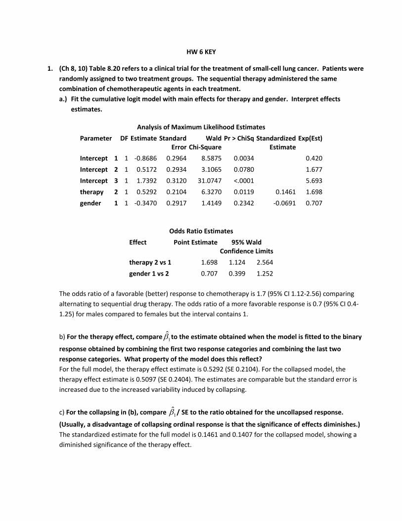
1. (Ch 8, 10) Table 8.20 refers to a clinical trial for the treatment of small-cell lung cancer. Patients were randomly assigned to two treatment groups. The sequential therapy administered the same combination of chemotherapeutic agents in each treatment. a.) Fit the cumulative logit model with main effects for therapy and gender. Interpret effects

estimates.

Analysis of Maximum Likelihood Estimates Parameter DF Estimate Standard

Error Wald

Chi-Square Pr > ChiSq Standardized

Estimate Exp(Est)

Intercept 1 1 -0.8686 0.2964 8.5875 0.0034 0.420 Intercept 2 1 0.5172 0.2934 3.1065 0.0780 1.677 Intercept 3 1 1.7392 0.3120 31.0747 <.0001 5.693 therapy 2 1 0.5292 0.2104 6.3270 0.0119 0.1461 1.698 gender 1 1 -0.3470 0.2917 1.4149 0.2342 -0.0691 0.707

Odds Ratio Estimates Effect Point Estimate 95% Wald

Confidence Limits therapy 2 vs 1 1.698 1.124 2.564 gender 1 vs 2 0.707 0.399 1.252

The odds ratio of a favorable (better) response to chemotherapy is 1.7 (95% CI 1.12-2.56) comparing alternating to sequential drug therapy. The odds ratio of a more favorable response is 0.7 (95% CI 0.4-1.25) for males compared to females but the interval contains 1.

b) For the therapy effect, compare 1̂β to the estimate obtained when the model is fitted to the binary

response obtained by combining the first two response categories and combining the last two response categories. What property of the model does this reflect? For the full model, the therapy effect estimate is 0.5292 (SE 0.2104). For the collapsed model, the therapy effect estimate is 0.5097 (SE 0.2404). The estimates are comparable but the standard error is increased due to the increased variability induced by collapsing.

c) For the collapsing in (b), compare 1̂β / SE to the ratio obtained for the uncollapsed response.

(Usually, a disadvantage of collapsing ordinal response is that the significance of effects diminishes.) The standardized estimate for the full model is 0.1461 and 0.1407 for the collapsed model, showing a diminished significance of the therapy effect.

d) Fit the model to the uncollapsed data that also contains an interaction term. Interpret. Does it fit better? Explain why it is equivalent to using the four gender-therapy combinations as levels of a single factor.

Analysis of Maximum Likelihood Estimates Parameter DF Estimate Standard

Error Wald

Chi-Square Pr > ChiSq Standardized

Estimate Exp(Est)

Intercept 1 1 -1.0112 0.3834 6.9578 0.0083 0.364 Intercept 2 1 0.3771 0.3791 0.9897 0.3198 1.458 Intercept 3 1 1.5990 0.3931 16.5487 <.0001 4.948 therapy 2 1 0.8510 0.5407 2.4775 0.1155 0.2350 2.342 gender 1 1 -0.1783 0.4072 0.1917 0.6615 -0.0355 0.837 therapy*gender 2 1 1 -0.3786 0.5852 0.4186 0.5176 -0.1031 0.685

No, it does not fit better. The interaction term is not significant (p=0.52) and the AIC and BIC are both lower for the model without the interaction term. The model with the interaction term assumes that the therapy effect is different across genders and gender effect is different across therapies. The inclusion of the interaction is equivalent to modeling a single, four-level fixed effect for the gender/therapy combinations and can be shown through the design matrix of the interaction model having four levels.

1 0 0 01 0 1 01 1 0 01 1 1 1

gender therapy gender therapyα β β β β×

data lung; input therapy gender resp1 resp2 cnt; label therapy='1=Seq 2=Alt' gender='1=male 2=female' resp1='1=bad 4=good' resp2='4=bad 1=good'; datalines; 1 1 1 4 28 1 1 2 3 45 1 1 3 2 29 1 1 4 1 26 1 2 1 4 4 1 2 3 2 12 1 2 2 3 5 1 2 1 4 2 2 1 1 4 41 2 1 2 3 44 2 1 3 2 20 2 1 4 1 20 2 2 1 4 12 2 2 3 2 7 2 2 2 3 3 2 2 4 1 1 ; run;

data lung1; set lung; if resp1=1 or resp1=2 then resp3=1; if resp1=3 or resp1=4 then resp3=2; do i=1 to cnt; output; end; run; proc logistic data=lung1; title1 'Full Model'; class therapy (ref='1') gender/param=ref; model resp1= therapy gender/stb expb; oddsratio therapy/diff=all; run; proc logistic data=lung1; title1 'Collapsed Model'; class therapy (ref='1') gender/param=ref; model resp3= therapy gender/stb expb; oddsratio therapy/diff=all; run; proc logistic data=lung1; title1 'Full Model with interaction'; class therapy (ref='1') gender/param=ref; model resp1= therapy gender therapy*gender/stb expb; oddsratio therapy/diff=all; run;

2. (Ch 8, 14) For Table 8.5, fit and interpret effects for a a. cumulative link model with complementary log-log link

1 1 2 2log[ log(1 ( | ))] jP Y j x xα β β− − ≤ = + +x

where Y = happiness (1=very happy, 2=pretty happy, 3=not too happy), 1x =# of traumatic events, and

2x =race (0=white, 1=black). The fitting result from SAS is shown below.

1 1 1 2 2 1 2log[ log(1 ( 1| ))] 0.9714 0.1999 0.9870P Y x x x xα β β− − ≤ = + + = − − −x

2 1 1 2 2 1 2log[ log(1 ( 2 | ))] 1.3674 0.1999 0.9870P Y x x x xα β β− − ≤ = + + = − −x

Interpretation for the standard cloglog link binary regression, specified by $log[-log(1-p)] = \beta_{1}x_{1}$ is already available. There, if estimate of $\beta_1$ is 0.15, then the probability of mortality per unit time, or the hazard, [which is P(Y=1|X)] is increased by 16% [because exp(0.15) = 1.162] for 1 unit increase in $x_{1}$. In this case, just replace your $p$ with $P(Y <= 1|X)$, i.e., ``the probability of remaining in the category 1, or less’’ per unit time.

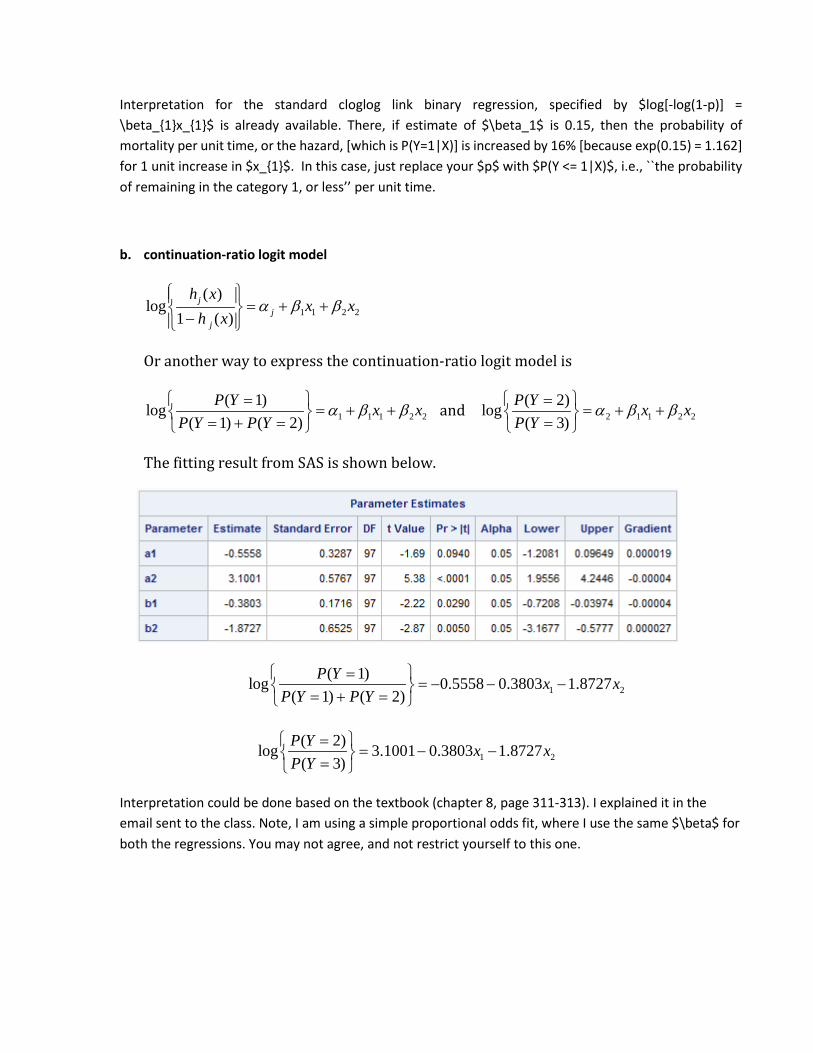
b. continuation-ratio logit model

1 1 2 2

( )log

1 ( )j

jj

h xx x

h xα β β

= + + −

Or another way to express the continuation-ratio logit model is

1 1 1 2 2( 1)log

( 1) ( 2)P Y x x

P Y P Yα β β

== + +

= + = and 2 1 1 2 2

( 2)log( 3)

P Y x xP Y

α β β =

= + + =

The fitting result from SAS is shown below.

1 2( 1)log 0.5558 0.3803 1.8727

( 1) ( 2)P Y x x

P Y P Y =

= − − − = + =

1 2( 2)log 3.1001 0.3803 1.8727( 3)

P Y x xP Y

== − −

=

Interpretation could be done based on the textbook (chapter 8, page 311-313). I explained it in the email sent to the class. Note, I am using a simple proportional odds fit, where I use the same $\beta$ for both the regressions. You may not agree, and not restrict yourself to this one.

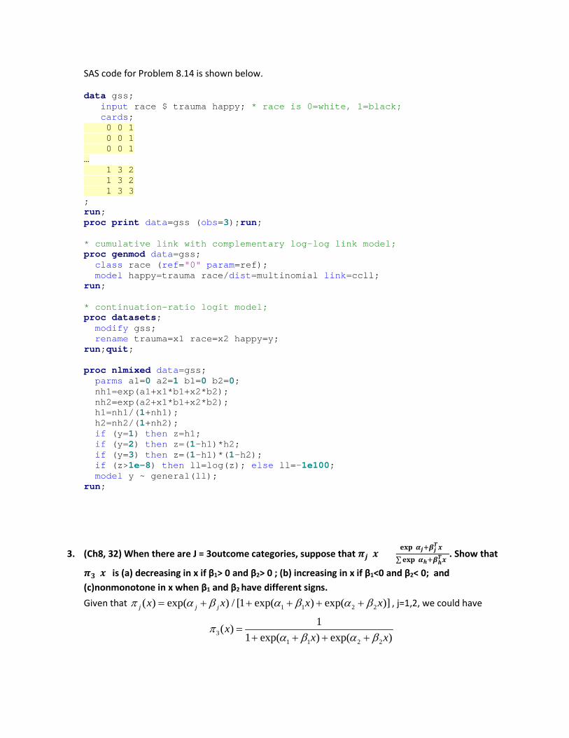
SAS code for Problem 8.14 is shown below.

data gss; input race $ trauma happy; * race is 0=white, 1=black; cards; 0 0 1 0 0 1 0 0 1 … 1 3 2 1 3 2 1 3 3 ; run; proc print data=gss (obs=3);run; * cumulative link with complementary log-log link model; proc genmod data=gss; class race (ref="0" param=ref); model happy=trauma race/dist=multinomial link=ccll; run; * continuation-ratio logit model; proc datasets; modify gss; rename trauma=x1 race=x2 happy=y; run;quit; proc nlmixed data=gss; parms a1=0 a2=1 b1=0 b2=0; nh1=exp(a1+x1*b1+x2*b2); nh2=exp(a2+x1*b1+x2*b2); h1=nh1/(1+nh1); h2=nh2/(1+nh2); if (y=1) then z=h1; if (y=2) then z=(1-h1)*h2; if (y=3) then z=(1-h1)*(1-h2); if (z>1e-8) then ll=log(z); else ll=-1e100; model y ~ general(ll); run;

3. (Ch8, 32) When there are J = 3outcome categories, suppose that 𝝅𝝅𝒋𝒋(𝒙𝒙) =𝐞𝐞𝐞𝐞𝐞𝐞 (𝜶𝜶𝒋𝒋+𝜷𝜷𝒋𝒋

𝑻𝑻𝒙𝒙)∑𝐞𝐞𝐞𝐞𝐞𝐞 (𝜶𝜶𝒉𝒉+𝜷𝜷𝒉𝒉

𝑻𝑻𝒙𝒙). Show that

𝝅𝝅𝟑𝟑(𝒙𝒙) is (a) decreasing in x if β1> 0 and β2> 0 ; (b) increasing in x if β1<0 and β2< 0; and (c)nonmonotone in x when β1 and β2 have different signs. Given that 1 1 2 2( ) exp( ) / [1 exp( ) exp( )]j j jx x x xπ α β α β α β= + + + + + , j=1,2, we could have

31 1 2 2

1( )1 exp( ) exp( )

xx x

πα β α β

=+ + + +

a. If 1β >0 and 2β > 0, 1 1exp( )xα β+ and 2 2exp( )xα β+ are both increasing as annual income (x)

increases which means the denominator of 3( )xπ increases as x increases. Therefore, 3( )xπ will be

decreasing in x if 1β >0 and 2β > 0.

b. If 1β <0 and 2β <0, 1 1exp( )xα β+ and 2 2exp( )xα β+ will be both decreasing as annual income (x)

increases which means that the denominator of 3( )xπ decreases as x increases. Therefore, 3( )xπ

will be increasing in x if 1β <0 and 2β <0.

c. If 1β and 2β have different signs, but we have no information about their magnitude or say absolute

values. So, we don’t know when x increases, how the denominator would change. Therefore, 3( )xπ

is non-monotone. A concrete example could help explain this:

Since 31 1 2 2

1( )1 exp( ) exp( )

xx x

πα β α β

=+ + + +

, its first derivative with respect to x is:

[ ]3 1 1 1 2 2 2

21 1 2 2

( ) [ exp( ) exp( )]1 exp( ) exp( )

x x xx x x

π β α β β α βα β α β

∂ − + + +=

∂ + + + +.

a. When β1> 0 and β2> 0, 𝜋𝜋3(𝑥𝑥) will decrease as x increases because the numerator will be increasingly negative and the denominator will be increasingly positive

b. When β1< 0 and β2< 0, 𝜋𝜋3(𝑥𝑥) will increase as x increases because the numerator will be increasingly positive (because of the negative sign) as will the denominator (because of the squared term)

c. When β1 and β2 have different signs, 𝜋𝜋3(𝑥𝑥) will be nonmonotone since it could increase or decrease as x increases depending on the relationship between β1 and β2 (i.e., 𝜋𝜋3(𝑥𝑥) will behave accordingly to the sign of the βj with the greatest magnitude)

4. (Ch11, 3) Table 11.14 shows data about belief in heaven and belief in hell. a. Compare the marginal proportions using a 95% CI

( ) ( )

11 21 11 121 1

( )

955 9 – 955 162 /1314

0.1164384

n n n nd p pn+ +++

+ − += − =

= + + = −

( ) ( )

212 21 12 21

2

ˆ ( ) [( ) ( ) ] /

= 162 /1314 9 /1314 – 162 /1314 – 9 /1314 1314

0.00942

d p p p p nσ ++= + − −

+ =

The 95% confidence interval is −0.1164 ± 1.96 × 0.0094 = (−0.135, −0.0980), which does not contain 0. It suggests that at 5% significance level, the difference between the marginal proportions are statistically significant.

b. Perform McNemar’s test and interpret results The McNemar chi-squared test statistic is 136.89, which corresponds to a p-value < 0.0001. Therefore,

we can conclude with 95% confidence that the marginal proportions are not equal.

c. Explain how these data suggest that the marginal proportions are strongly dependent rather than

independent. Explain why inferences in a) are more precise If the proportions are dependent,

( ) ( ) ( )1 1 1 1 11 22 12 21Var( ) 1 1 2n d π π π π π π π π+ + + += − + − − −

If the proportions are independent,

( ) ( )1 1 1 1Var( ) 1 1n d π π π π+ + + += − + −

( )11 22 12 21 0.103π π π π− = , so 11 22 12 21π π π π> indicating that the response is positively correlated,

and the variance is smaller relative to two independent samples. Based on the texbook Page 414-

416, these proportions are correlated.

5. (ch11, 7) A case-control study has 8 pairs of subjects. The cases have colon cancer, and the controls are matched with the cases on gender and age. A possible explanatory variable is the extent of red meat in a subject’s diet, measured as “1=high” or “0=low.” The (case, control) observations on this were (1,1) for 3 pairs, (0,0) for 1 pair, (1,0) for 3 pairs and (0,1) for 1 pair. Perform a conditional analysis in proc logistic using the strata and exact commands and interpret the results. The estimate of β is 1.0986. Therefore the odds of people who eat high levels of red meat develop colon cancer is exp(1.0986) ≈ 3 times the odds of developing colon cancer for people who eat low levels of red meat. However, the effect of red meat is not statistically significant, since the 95% C.I. for the odds ratio includes 1.

6. Ch(12, 8) Refer to Table 13.3 in Section 13.3.2 on attitudes toward legalized abortion. For the response Yt(1=support legalization, 0=oppose) for question t (t=1,2 ,3) and gender g (1=female, 0=male), consider the model: logit[P(Yt=1)]=α+γg+βt with β3=0. a. A GEE analysis using unstructured working correlation gives correlation estimates 0.826 for

questions 1 and 2, 0.797 for 1 and 3 and 0.832 for 2 and 3. What does this suggest about a reasonable working correlation structure? Why? Since the correlations are all roughly the same, we could use an exchangeable correlation structure.

b. Table 12.12 shows a GEE analysis with exchangeable working correlation. Interpret effects The odds of supporting the legalization of abortion were exp(0.15) = 1.16 times higher for question one, which was statistically significant when compared to question 3. The odds of supporting the legalization were exp(0.052) = 1.05 times higher with question two, which was marginally significant when compared to question 3. The odds were lowest for question 3. The odds of supporting legalization were exp(0.0034) = 1.003 times higher for women, but that was not significantly higher than men. The correlation between supporting legalization on one question was strongly positively correlated with supporting abortion on the other two questions.

c. Treating the three responses for each subject as independent observations and performing

ordinary logistic regression. β1=0.149 (SE=0.066), β2=0.052 (SE=0.066), γ=0.004 (SE=0.054). Give a heuristic explanation of why within-subject SEs are much larger than with GEE, yet the between-subject SE is smaller.

There is a very high positive correlation between answers to questions for a given subject. This

correlation reduces to the within-subject standard errors when comparing two questions, because

( ) ( ), 0ij ikCov E Y E Y > with positive correlation and

( ) ( )ij ikVar E Y E Y − = ( ) ( )ij ikVar E Y Var E Y + ( ) ( ),ij ikCov E Y E Y − .

Thus, positive correlation reduces the within-subject comparison variance ( ) ( )ij ikVar E Y E Y −

and the corresponding standard errors.

Similarly, this positive correlation increases the between-subject comparison standard errors,

because the answers from each subject are independent and

( ) ( )ij ikVar E Y E Y + = ( ) ( )ij ikVar E Y Var E Y + ( ) ( ),ij ikCov E Y E Y + .

Thus, ( ) ( ) ( ) ( ){ }ij ik lj lkVar E Y E Y E Y E Y + − + will be generally increased.

7. (Ch12, 10) Use GEE methods to analyze the clinical trials data in Table 13.7, treating observations within each center as a correlated cluster.

Exchangeable Working Correlation ρ̂ = 0.2169

Score Statistics For Type 3 GEE Analysis

Score Statistics For Type 3 GEE Analysis:

Chi-

Source DF Square Pr > ChiSq

treat 1 3.43 0.0641

Using GEE methods with an exchangeable correlation matrix to model the success of treatment we found

that averaged over centers the estimated odds of success for a subject given the drug is exp(0.554)=1.7402

times the estimated odds of a subject given the placebo. Since the p-value for the covariate treat is smaller

than 0.05, we conclude with 95% confidence that there is evidence that the drug produces better results

than the control.

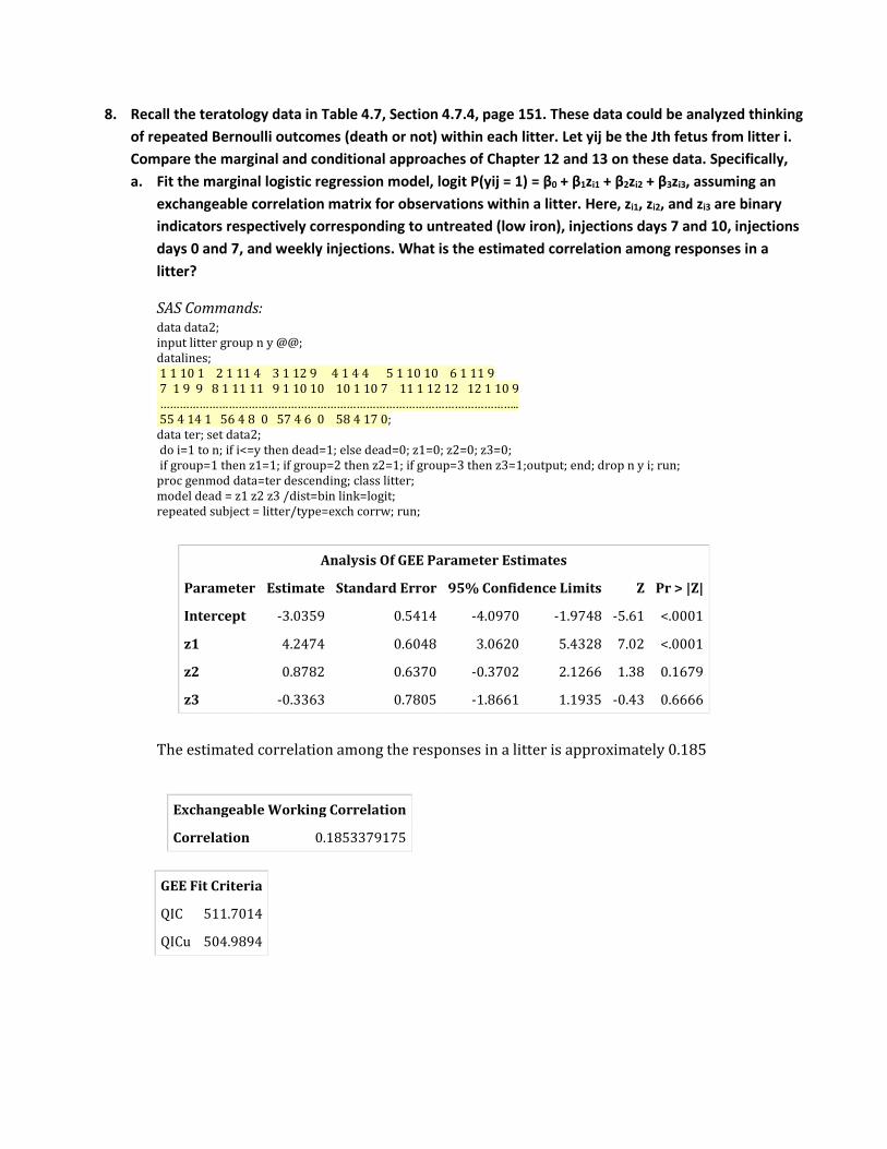
8. Recall the teratology data in Table 4.7, Section 4.7.4, page 151. These data could be analyzed thinking of repeated Bernoulli outcomes (death or not) within each litter. Let yij be the Jth fetus from litter i. Compare the marginal and conditional approaches of Chapter 12 and 13 on these data. Specifically, a. Fit the marginal logistic regression model, logit P(yij = 1) = β0 + β1zi1 + β2zi2 + β3zi3, assuming an

exchangeable correlation matrix for observations within a litter. Here, zi1, zi2, and zi3 are binary indicators respectively corresponding to untreated (low iron), injections days 7 and 10, injections days 0 and 7, and weekly injections. What is the estimated correlation among responses in a litter?

SAS Commands: data data2; input litter group n y @@; datalines; 1 1 10 1 2 1 11 4 3 1 12 9 4 1 4 4 5 1 10 10 6 1 11 9 7 1 9 9 8 1 11 11 9 1 10 10 10 1 10 7 11 1 12 12 12 1 10 9 ……………………………………………………………………………………………….. 55 4 14 1 56 4 8 0 57 4 6 0 58 4 17 0; data ter; set data2; do i=1 to n; if i<=y then dead=1; else dead=0; z1=0; z2=0; z3=0; if group=1 then z1=1; if group=2 then z2=1; if group=3 then z3=1;output; end; drop n y i; run; proc genmod data=ter descending; class litter; model dead = z1 z2 z3 /dist=bin link=logit; repeated subject = litter/type=exch corrw; run;

The estimated correlation among the responses in a litter is approximately 0.185

Analysis Of GEE Parameter Estimates

Parameter Estimate Standard Error 95% Confidence Limits Z Pr > |Z|

Intercept -3.0359 0.5414 -4.0970 -1.9748 -5.61 <.0001

z1 4.2474 0.6048 3.0620 5.4328 7.02 <.0001

z2 0.8782 0.6370 -0.3702 2.1266 1.38 0.1679

z3 -0.3363 0.7805 -1.8661 1.1935 -0.43 0.6666

Exchangeable Working Correlation

Correlation 0.1853379175

GEE Fit Criteria

QIC 511.7014

QICu 504.9894

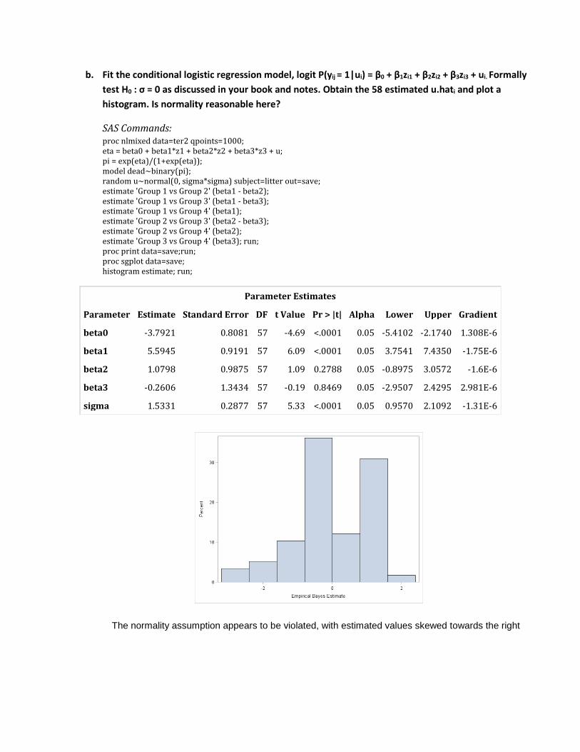
b. Fit the conditional logistic regression model, logit P(yij = 1|ui) = β0 + β1zi1 + β2zi2 + β3zi3 + ui. Formally test H0 : σ = 0 as discussed in your book and notes. Obtain the 58 estimated u.hati and plot a histogram. Is normality reasonable here?

SAS Commands: proc nlmixed data=ter2 qpoints=1000; eta = beta0 + beta1*z1 + beta2*z2 + beta3*z3 + u; pi = exp(eta)/(1+exp(eta)); model dead~binary(pi); random u~normal(0, sigma*sigma) subject=litter out=save; estimate 'Group 1 vs Group 2' (beta1 - beta2); estimate 'Group 1 vs Group 3' (beta1 - beta3); estimate 'Group 1 vs Group 4' (beta1); estimate 'Group 2 vs Group 3' (beta2 - beta3); estimate 'Group 2 vs Group 4' (beta2); estimate 'Group 3 vs Group 4' (beta3); run; proc print data=save;run; proc sgplot data=save; histogram estimate; run;

Parameter Estimates

Parameter Estimate Standard Error DF t Value Pr > |t| Alpha Lower Upper Gradient

beta0 -3.7921 0.8081 57 -4.69 <.0001 0.05 -5.4102 -2.1740 1.308E-6

beta1 5.5945 0.9191 57 6.09 <.0001 0.05 3.7541 7.4350 -1.75E-6

beta2 1.0798 0.9875 57 1.09 0.2788 0.05 -0.8975 3.0572 -1.6E-6

beta3 -0.2606 1.3434 57 -0.19 0.8469 0.05 -2.9507 2.4295 2.981E-6

sigma 1.5331 0.2877 57 5.33 <.0001 0.05 0.9570 2.1092 -1.31E-6

The normality assumption appears to be violated, with estimated values skewed towards the right

c. Compare and interpret the results. In particular, how does the interpretation change from marginal to conditional? Report the 6 pairwise odds ratios and confidence intervals for comparison across the four treatment groups. Which are significant and which are not? Interpret in terms of how odds of death change.

The interpretation of the marginal results are in terms of the odds of the outcome averaged for the group (in this case, the litter) while the conditional results are interpreted in terms of the odds of the outcome for a typical individual regardless of group membership (in this case, the fetus):

Marginal Interpretation: eβ = e4.2474 = 69.92

The odds of death in the litter were 69.92 times higher if the fetuses were injected at 7 and 10 weeks.

Conditional Interpretation: eβ = e5.5954 = 269.19

The odds of death in a typical fetus were 269.19 times higher if the fetus was injected at 7 and 10 weeks.

Non-significant predictors were not significant in both the marginal and conditional models.

Additional Estimates

Label Estimate Standard Error DF t Value Pr > |t| Alpha Lower Upper

Group 1 vs Group 2 4.5147 0.7360 57 6.13 <.0001 0.05 3.0409 5.9885

Group 1 vs Group 3 5.8551 1.1899 57 4.92 <.0001 0.05 3.4724 8.2378

Group 1 vs Group 4 5.5945 0.9191 57 6.09 <.0001 0.05 3.7541 7.4350

Group 2 vs Group 3 1.3404 1.2513 57 1.07 0.2886 0.05 -1.1652 3.8461

Group 2 vs Group 4 1.0798 0.9875 57 1.09 0.2788 0.05 -0.8975 3.0572

Group 3 vs Group 4 -0.2606 1.3434 57 -0.19 0.8469 0.05 -2.9507 2.4295

For Group 1 vs. Group 2: eβ = e4.5147 = 91.35; 95% CI = (e4.5147 +/- 1.96SE) = (21.59, 386.55)

For Group 1 vs. Group 3: eβ = e5.8551= 349.01; 95% CI = (e5.8551+/- 1.96SE) = (33.88, 3595.02)

For Group 1 vs. Group 4: eβ = e5.5945 = 268.94; 95% CI = (e5.5945 +/- 1.96SE) = (44.39, 1629.35)

The following estimates are not significant at the 95% confidence level-- their 95% CIs contain the null value “1”

For Group 2 vs. Group 3: eβ = e1.3404 = 3.82; 95% CI = (e1.3404+/- 1.96SE) = (0.329, 44.39)

For Group 2 vs. Group 4: eβ = e1.0798 = 2.94; 95% CI = (e1.0798 +/- 1.96SE) = (0.425, 20.40)

For Group 2 vs. Group 4: eβ = e-0.2606 = 0.77; 95% CI = (e-0.2606 +/- 1.96SE) = (0.055, 10.72)

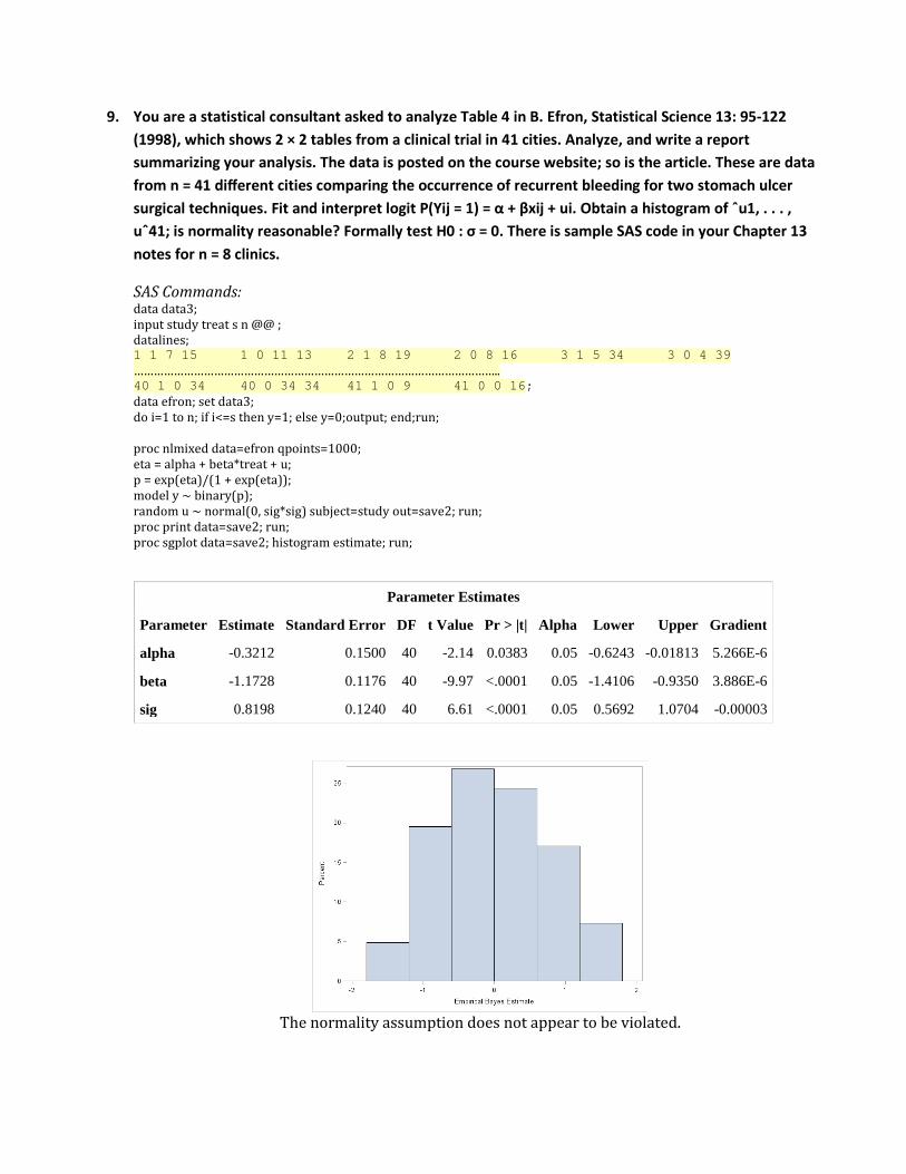
9. You are a statistical consultant asked to analyze Table 4 in B. Efron, Statistical Science 13: 95-122 (1998), which shows 2 × 2 tables from a clinical trial in 41 cities. Analyze, and write a report summarizing your analysis. The data is posted on the course website; so is the article. These are data from n = 41 different cities comparing the occurrence of recurrent bleeding for two stomach ulcer surgical techniques. Fit and interpret logit P(Yij = 1) = α + βxij + ui. Obtain a histogram of ˆu1, . . . , uˆ41; is normality reasonable? Formally test H0 : σ = 0. There is sample SAS code in your Chapter 13 notes for n = 8 clinics.

SAS Commands: data data3; input study treat s n @@ ; datalines; 1 1 7 15 1 0 11 13 2 1 8 19 2 0 8 16 3 1 5 34 3 0 4 39 ……………………………………………………………………………………………….. 40 1 0 34 40 0 34 34 41 1 0 9 41 0 0 16; data efron; set data3; do i=1 to n; if i<=s then y=1; else y=0;output; end;run; proc nlmixed data=efron qpoints=1000; eta = alpha + beta*treat + u; p = exp(eta)/(1 + exp(eta)); model y ~ binary(p); random u ~ normal(0, sig*sig) subject=study out=save2; run; proc print data=save2; run; proc sgplot data=save2; histogram estimate; run;

Parameter Estimates

Parameter Estimate Standard Error DF t Value Pr > |t| Alpha Lower Upper Gradient

alpha -0.3212 0.1500 40 -2.14 0.0383 0.05 -0.6243 -0.01813 5.266E-6

beta -1.1728 0.1176 40 -9.97 <.0001 0.05 -1.4106 -0.9350 3.886E-6

sig 0.8198 0.1240 40 6.61 <.0001 0.05 0.5692 1.0704 -0.00003

The normality assumption does not appear to be violated.