hurst, martin d., mudd, simon m., yoo, kyungsoo, attal

Hurst, Martin D., Mudd, Simon M., Yoo, Kyungsoo, Attal, Mikael and Walcott, Rachel. (2014) Influence of lithology on hillslope morphology and response to tectonic forcing in the Sierra Nevada of California. Journal of Geophysical Research: Earth Surface, Vol.118 NO.2 (2013) pp.832-851 DOI: 10.1002/jgrf.20049 http://repository.nms.ac.uk/1106 Deposited on: 03 November 2014

NMS Repository – Research publications by staff of the National Museums Scotland

http://repository.nms.ac.uk/

Influence of lithology on hillslope morphology and responseto tectonic forcing in the northern Sierra Nevada of California

Martin D. Hurst,1,2 Simon M. Mudd,1,3 Kyungsoo Yoo,4 Mikael Attal,1

and Rachel Walcott1,5

Received 6 February 2012; revised 13 February 2013; accepted 15 February 2013; published 24 May 2013.

[1] Many geomorphic studies assume that bedrock geology is not a first-order control onlandscape form in order to isolate drivers of geomorphic change (e.g., climate or tectonics).Yet underlying geology may influence the efficacy of soil production and sedimenttransport on hillslopes. We performed quantitative analysis of LiDAR digital terrainmodels to examine the topographic form of hillslopes in two distinct lithologies in theFeather River catchment in northern California, a granodiorite pluton and metamorphosedvolcanics. The two sites, separated by <2 km and spanning similar elevations, wereassumed to have similar climatic histories and are experiencing a transience in landscapeevolution characterized by a propagating incision wave in response to accelerated surfaceuplift c. 5 Ma. Responding to increased incision rates, hillslopes in granodiorite tend tohave morphology similar to model predictions for steady state hillslopes, suggesting thatthey adjust rapidly to keep pace with the incision wave. By contrast, hillslopes inmetavolcanics exhibit high gradients but lower hilltop curvature indicative of ongoingtransient adjustment to incision. We used existing erosion rate data and the curvature ofhilltops proximal to the main channels (where hillslopes have most likely adjusted toaccelerated erosion rates) to demonstrate that the sediment transport coefficient is higher ingranodiorite (8.8 m2 ka�1) than in metavolcanics (4.8 m2 ka�1). Hillslopes in bothlithologies get shorter (i.e., drainage density increases) with increasing erosion rates.

Citation: Hurst, M. D., S. M. Mudd, K. Yoo, M. Attal, and R. Walcott (2013), Influence of lithology on hillslopemorphology and response to tectonic forcing in the northern Sierra Nevada of California, J. Geophys. Res. Earth Surf.,

118, 832–851, doi:10.1002/jgrf.20049.

1. Introduction

[2] Climate and tectonics act in concert to control themorphology of the Earth’s surface. The ability to quantifyrelationships between topography and climatic or tectonicdriving processes is dependent on understanding how effi-ciently, and by which processes, sediment is generated andtransported on hillslopes and in valleys [e.g., Ahnert, 1970;Dietrich et al., 2003]. Such knowledge is vital for ongoing

modeling efforts which help link empirical observations totheoretical predictions [e.g., Tucker and Hancock, 2010].Hillslope processes control the flux and caliber of sedimentsupplied to streams [e.g., Whittaker et al., 2010], whichsubsequently influence fluvial incision rates [e.g., Sklar andDietrich, 2004] and the rate at which sediment is deliveredto basins [e.g., Duller et al., 2010; Armitage et al., 2011].[3] Tectonic processes redistribute rock mass within the

lithosphere and control the type and flux of rock materialexhumed to the surface. This material may be weakened atdepth via mechanical fracturing due to tectonic processes[e.g., Molnar et al., 2007] and later disrupted at/near thesurface by physical and chemical weathering processes(e.g., penetration and growth of tree roots [Roering et al.,2010; Gabet and Mudd, 2010], frost wedging [e.g., Smallet al., 1999], and chemical alteration and weakening [e.g.,Burke et al., 2007; Dixon et al., 2009]). These processesgenerate soil/regolith, here used synonymously and definedas material at or near the Earth’s surface that is being phys-ically disturbed (equivalent to the physically disturbed zoneas defined by Yoo and Mudd [2008]) and which can besubsequently transported away. The type and physical prop-erties (composition, rock mass strength, and degree of frac-turing) of bedrock will influence the physical properties ofthe resulting soil (e.g., composition, grain size distribution,

1School of Geosciences, University of Edinburgh, Edinburgh, UK.2British Geological Survey, Nottingham, UK.3Earth Research Institute, University of California, Santa Barbara,

California, USA.4Department of Soil, Water, and Climate, University of Minnesota,

St. Paul, Minnesota, USA.5Department of Natural Sciences, National Museums Scotland,

Edinburgh, UK.

Corresponding author: M. D. Hurst, British Geological Survey, NickerHill, Keyworth, Nottingham NG12 5GG, UK. ([email protected])

©2013 The Authors. Journal of Geophysical Research: Earth Surfacepublished by Wiley on behalf of the American Geophysical Union.This is an open access article under the terms of the Creative CommonsAttribution License, which permits use, distribution and reproduction inany medium, provided the original work is properly cited.2169-9003/13/10.1002/jgrf.20049

832

JOURNAL OF GEOPHYSICAL RESEARCH: EARTH SURFACE, VOL. 118, 832–851, doi:10.1002/jgrf.20049, 2013

http://creativecommons.org/licenses/by/3.0/

http://creativecommons.org/licenses/by/3.0/

degree of weathering, porosity, and cohesion [Yoo et al.,2005]). The physical characteristics of soil are in turnexpected to influence the efficacy at which sediment trans-port occurs on hillslopes [Furbish et al., 2009]. Thus, thereis the potential for bedrock lithology to influence topographyeven in soil-mantled landscapes.[4] Several studies have attempted to quantify relation-

ships between rock strength and topography, or have consid-ered the role that spatially variable rock type may have incontrolling processes which generate and redistribute sedi-ment at the Earth’s surface. Schmidt and Montgomery[1995] demonstrated that hillslope relief is limited by the ma-terial strength of bedrock. Similarly, Burbank et al. [1996]suggested that hillslope gradients were limited at their in-ternal friction angle, despite variation of over an order ofmagnitude in denudation rates in the northwest Himalayas(1–12 mm a�1). Hillslopes were thus interpreted to evolvein response to variable erosion rates by adjusting the fre-quency of landslides rather than by steepening. The distribu-tion of slope angles may serve as a proxy for rock massstrength in landslide-dominated terrain as demonstrated byKorup [2008] and Korup and Schlunegger [2009]. Clarkeand Burbank [2010] however were not able to distinguishrock mass strength from hillslope gradients in distinct lithol-ogies in Southern New Zealand. They attributed the similar-ities between low-grade metamorphics of the Southern Alpsand high-grade and igneous units of the Fiordland to the na-ture of bedrock fracturing. Both sites are susceptible tolandsliding, but different styles of fracturing were interpretedto control the type of mass wasting process operating. InFiordland, fracturing occurs primarily due to near surfaceprocesses and thus drives frequent shallow landslides,whereas pervasive tectonic fracturing in the Southern Alpsfacilitates larger, deeper landsides [Clarke and Burbank,2010; 2011]. Although links between bedrock lithology andtopography have been explored in bedrock landscapes, nostudies have explored the role that lithology may play in con-trolling topography in soil-mantled landscapes.[5] Lithology may play an important role in controlling

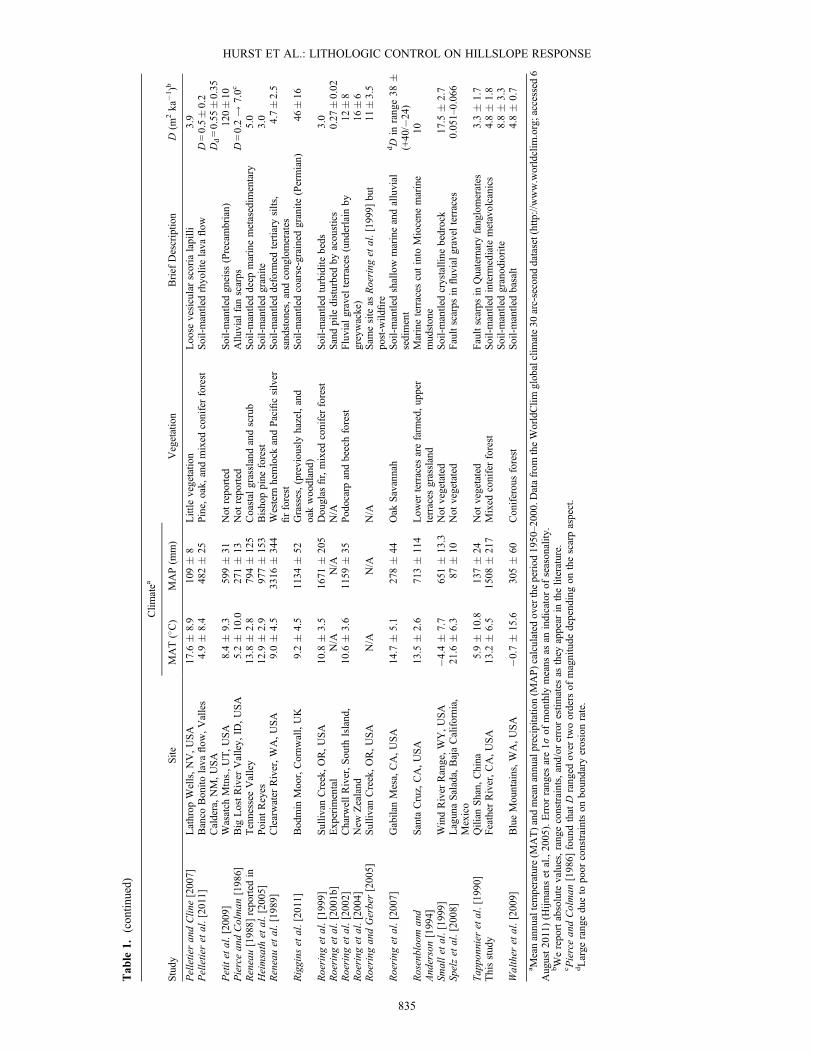
the efficiency of sediment transport on hillslopes. McKeanet al. [1993] showed that the sediment transport coefficientD, which relates hillslope gradient to sediment flux, is anorder of magnitude larger in weak clay-rich soils than instrong, granular soils, presumably due to variation in theefficiency of shrink-swell cycles as a transport process. Thisis at least partially controlled by the parent lithology throughthe nature of jointing and susceptibility to weathering.Furbish et al. [2009] described the sediment transport coef-ficient D as a function of the material properties of soilincluding thickness, grain size distribution, and cohesionwhich may directly influence the efficiency of sedimenttransport. The presence of coarse material in the soil mayresult in a boulder lag which armours underlying soil fromerosion [e.g., Granger et al., 2001]. Owen et al., 2010demonstrated that hillslope erosion rates across a climategradient in Chile were sensitive to precipitation, which influ-ences transport processes, with more rapid erosion rateattributed to wetter climate and biologically driven sedimenttransport. To assess whether there is any existing evidencethat D might be influenced by lithology, we compiled pub-lished values of D to search for global trends with lithology(Figure 1a and Table 1). Simplifying to cohesionless, clastic,

volcanic, and crystalline lithologic groups, we were not ableto observe any trends between lithology and the sedimenttransport coefficient (Figure 1b). However, isolating forvalues derived from cohesionless substrate (i.e., alluvium;n = 24), we observe that D increases with precipitation and

(a)

(b)

(c)

Figure 1. (a) Global distribution of calibrated sediment trans-port coefficients (red) (Table 1). (b) Mean annual precipitationplotted against calibrated sediment transport coefficients forlithologic groups. In unconsolidated substrate, there is a weaktendency for D to increase with wetter climate (R2 = 0.27 forlinear regression). (c) Sediment transport efficiency vs. annualvariability of precipitation (2s about mean monthly precipita-tion). D increases with more variable intra-annual precipitation(R2 = 0.51 for linear regression). There were no trends observedwhen comparing D to mean annual temperature.

HURST ET AL.: LITHOLOGIC CONTROL ON HILLSLOPE RESPONSE

833

Tab

le1.

ReportedValuesof

theSedim

entTransportCoefficientD

andAssociatedCrude

Clim

ateData;

Includes

Brief

Descriptio

nsof

VegetationTypeandSubstrate

Material

Study

Site

Clim

atea

Vegetation

Brief

Descriptio

nD

(m2ka

�1)b

MAT(�C)

MAP(m

m)

Almondet

al.[2008]

Charw

ellBasin,New

Zealand

10.6

�3.6

1159

�35

Grassland/shrubland

Fluvial

gravel

terraces

3.0�

1.0

Podocarp/beechforest

5.0�

2.0

Almondet

al.[2008]

Ahuriri,New

Zealand

11.8

�3.9

662�

22Grassland/shrubland

Thick

loessdeposits(underlain

byaltered

basalt)

3.1�

0.4

Recentpasturegrasses

7.0�

2.0

Arrow

smith

etal.[1998]

Carrizo

Plain,CA,USA

14.5

�6.2

475�

73Grasses

andshrubs

Faultscarps

inalluvial

gravel

8.6�

0.8

Avouacet

al.[1993]

TienShan,

China

9.5�

14.2

138�

13Grasses

andshrubs

Faultscarps

inalluvial

gravel

5.5�

2.0

AvouacandPeltzer

[1993]

Hotan

Region,

Xinjiang,China

1.8�

10.7

33�

6Not

vegetated

Faultscarps

inalluvial

gravel

3.3�

1.4

Begin

[1992]

NorthernNegev,Israel

19.6

�5.0

193�

36Not

vegetated

Fluvial

gravel

terraces

0.4�

0.3

Bow

man

andGerson[1986]

LakeLisan,DeadSea

24.3

�6.5

142�

27Not

vegetated

Laketerraces

0.4

Bow

man

andGross

[1989]

asreported

inHanks

[2000]

NorthernArava,Israel

18.8

�5.5

198�

37Not

vegetated

Faultscarps

inalluvial

gravel

>0.4

Carretieret

al.[2002]

GurvanBugdfaultsystem

,Mongolia

0.3�

12.2

160�

33Not

vegetated

Faultscarps

inalluvial

gravel

3.3�

1.7

Colman

andWatson[1983]

LakeBonneville,UT,USA

9.5�

9.2

456�

19Grasses

andshrubs

Allu

vial

shorelinescarps

0.9

Constantin

eet

al.[2012]

Sim

ulated

Douglas

FirForest

N/A

N/A

Douglas

Fir

N/A

0.1–3.5

Enzel

etal.[1996]

SouthernArava

Valley,

Israel

24.2

�6.3

32�

6Not

vegetated

Faultscarps

inalluvial

gravel

0.2–0.3

Gabet

[2000]

TransverseRanges,CA,USA

15.0

�4.0

498�

83Coastal

Sage

Plio

-Pleistocene

fanglomerates.

Process

specific:

gopher

bioturbatio

n7.4

Gabet

[2003]

TransverseRanges,CA,USA

15.0

�4.0

498�

83Coastal

Sage

Plio

-Pleistocene

fanglomerates.

Process

specific:

dryravel

0.17

Hanks

etal.[1984]


9.5�

9.2

456�

19Grasses

andshrubs

Allu

vial

shorelinescarps

1.1

Hanks

etal.[1984]

Santa

Cruzseacliffs,CA,USA

13.8

�2.8

693�

111

Low

erterraces

arefarm

ed,upper

terraces

grassland

Quaternarywave-cutterraces

cutinto

Plio

cene

mudstone

11

Hanks

etal.[1984]

RaymondFaultScarp,LA,

CA,USA

18.1

�4.2

450�

76Not

reported

Faultscarps

inalluvial

gravel

16

Hanks

etal.[1984]

Drum

Mtns.,UT,USA

10.1

�9.9

192�

10Low

shrubs

(sagebrush

andshadscale)

7–20%

cover

Faultscarps

inalluvial

gravel

1.1

Hanks

andWallace

[1985]

LakeLahonta,NV,USA

10.0

�8.5

202�

9Not

reported

Allu

vial

shorelinescarps

1.1

Hanks

[2000]

LostRiver,ID

,USA

3.3�

9.1

270�

16Not

reported

Faultscarps

inalluvial

gravel

0.9–1.0

Heimsath

etal.[2000]

Nunnock

River,SEAustralia

12.8

�4.4

827�

32Schlerophyllforest

Soil-mantledgranite

4.0

Heimsath

etal.[2005]

Nunnock

River,SEAustralia

12.8

�4.4

827�

32Schlerophyllforest

Soil-mantledgranite

Dd=5.5m

ka�1

Tennessee

Valley,

CA,USA

13.8

�2.8

794�

125

Coastal

grasslandandscrub

Soil-mantleddeep

marinemetasedim

entary

Dd=1.25

mka

�1

Point

Reyes,CA,USA

12.9

�2.9

977�

153

Bishoppine

forest

Soil-mantledgranite

Dd=0.5m

ka�1

Hughesetal.[2009]

Charw

ellBasin,New

Zealand

N/A

N/A

Shrubland/grassland

(latePleistocene)

Fluvial

gravel

terraces

(underlain

bygreywacke)

4.7�

2.0

10.6

�3.6

1159

�35

Podocarpandbeechforest

8.8�

3.0

Hurstet

al.[2012]

Feather

River,CA,USA

13.2

�6.5

1508

�217

Mixed

coniferforest

Soil-mantledgranito

ids

8.0

Jungerset

al.[2009]

Great

Smokey

Mountains,NC,USA

8.4�

7.3

1855

�24.1

Deciduous

forest

Soil-mantledquartzite

6.5–10

Martin

andChurch[1997]

Various

N/A

N/A

Various

From

fieldmeasurementsof

volumetric

creeprates

0.2

Mattson

andBruhn

[2001]


9.5�

9.2

456�

19Grasses

andshrubs

Allu

vial

shorelinescarps

1.2�

0.3

Mattson

andBruhn

[2001]

Wasatch

FaultZone,UT,USA

9.5�

9.3

420�

17Not

reported

Faultscraps

inalluvial

gravel

2.8�

1.1

McK

eanet

al.[1993]

EastBay

RegionalPark,

CA,USA

14.9

�5.4

522�

79Grasses,clay-richsoil

Soil-mantledEocenemarineshale

36�

5Nash[1980a]

Emmet

County,

MI,USA

5.7�

10.1

825�

35Mixed

pine,oak,

beechforest

Wave-cutterraces

inmoraine

12Nash[1980b]

Drum

Mtns.,UT,USA

10.1

�9.9

192�

10Low

shrubs

(sagebrush

andshadscale)

7–20%

cover

Faultscarps

inalluvial

gravel

0.4

Nash[1984]

HebgenLake,MT,USA

1.9�

9.6

615�

22Not

reported

Faultscarps

inalluvial

gravel

andfluvial

gravel

terraces

2.0�0.4

Nivière

andMarquis[2000]

Upper

Rhine

Graben,

Germany

10.2

�6.6

707�

32Forested

Fluvial

gravel

terraces

1.4

Pelletieret

al.[2006]


9.5�

9.2

456�

19Grasses

andshrubs

Allu

vial

shorelinescarps

1.0


834

Tab

le1.

(contin

ued)

Study

Site

Clim

atea

Vegetation

Brief

Descriptio

nD

(m2ka

�1)b

MAT(�C)

MAP(m

m)

PelletierandClin

e[2007]

Lathrop

Wells,NV,U

SA

17.6

�8.9

109�

8Little

vegetatio

nLoose

vesicularscoria

lapilli

3.9

Pelletieret

al.[2011]

Banco

Bonito

lava

flow

,Valles

Caldera,NM,USA

4.9�

8.4

482�

25Pine,oak,

andmixed

coniferforest

Soil-mantledrhyolitelava

flow

D=0.5�0.2

Dd=0.55

�0.35

Petitet

al.[2009]

Wasatch

Mtns.,UT,USA

8.4�

9.3

599�

31Not

reported

Soil-mantledgneiss

(Precambrian)

120�10

PierceandColman

[1986]

Big

LostRiver

Valley,

ID,USA

5.2�

10.0

271�

13Not

reported

Allu

vial

fanscarps

D=0.2!

7.0c

Reneau[1988]

reported

inHeimsath

etal.[2005]

Tennessee

Valley

13.8

�2.8

794�

125

Coastal

grasslandandscrub

Soil-mantleddeep

marinemetasedim

entary

5.0

Point

Reyes

12.9

�2.9

977�

153

Bishoppine

forest

Soil-mantledgranite

3.0

Reneauet

al.[1989]

Clearwater

River,WA,USA

9.0�

4.5

3316

�344

Western

hemlock

andPacificsilver

firforest

Soil-mantleddeform

edtertiary

silts,

sandstones,andconglomerates

4.7�2.5

Riggins

etal.[2011]

Bodmin

Moor,Cornw

all,UK

9.2�

4.5

1134

�52

Grasses,(previouslyhazel,and

oakwoodland)

Soil-mantledcoarse-grained

granite

(Permian)

46�16

Roering

etal.[1999]

Sulliv

anCreek,OR,USA

10.8

�3.5

1671

�205

Douglas

fir,mixed

coniferforest

Soil-mantledturbidite

beds

3.0

Roering

etal.[2001b]

Experim

ental

N/A

N/A

N/A

Sandpile

disturbedby

acoustics

0.27

�0.02

Roering

etal.[2002]

Charw

ellRiver,South

Island,

New

Zealand

10.6

�3.6

1159

�35

Podocarpandbeechforest

Fluvial

gravel

terraces

(underlain

bygreywacke)

12�8

Roering

etal.[2004]

16�6

Roering

andGerber[2005]

Sulliv

anCreek,OR,USA

N/A

N/A

N/A

Sam

esite

asRoering

etal.[1999]

but

post-w

ildfire

11�3.5

Roering

etal.[2007]

GabilanMesa,CA,USA

14.7

�5.1

278�

44Oak

Savannah

Soil-mantledshallow

marineandalluvial

sediment

dD

inrange38

�(+40/�

24)

Rosenbloom

and

Anderson[1994]

Santa

Cruz,CA,USA

13.5

�2.6

713�

114

Low

erterraces

arefarm

ed,upper

terraces

grassland

Marineterraces

cutinto

Miocene

marine

mudstone

10

Smallet

al.[1999]

WindRiver

Range,WY,USA

�4.4

�7.7

651�

13.3

Not

vegetated

Soil-mantledcrystalline

bedrock

17.5

�2.7

Spelzetal.[2008]

LagunaSalada,BajaCalifornia,

Mexico

21.6

�6.3

87�

10Not

vegetated

Faultscarps

influvialgravel

terraces

0.051–0.066

Tapponnieretal.[1990]

Qilian

Shan,

China

5.9�

10.8

137�

24Not

vegetated

Faultscarps

inQuaternaryfanglomerates

3.3�

1.7

Thisstudy

Feather

River,CA,USA

13.2

�6.5

1508

�217

Mixed

coniferforest

Soil-mantledinterm

ediate

metavolcanics

4.8�

1.8

Soil-mantledgranodiorite

8.8�

3.3

Walther

etal.[2009]

BlueMountains,WA,USA

�0.7

�15.6

305�

60Coniferousforest

Soil-mantledbasalt

4.8�

0.7

a Meanannualtemperature(M

AT)andmeanannualprecipitatio

n(M

AP)calculated

overtheperiod

1950–2000.Datafrom

theWorldClim

globalclim

ate30

arc-second

dataset(http://www.worldclim

.org;accessed6

August2011)(H

ijmanset

al.,2005).Error

ranges

are1s

ofmonthly

means

asan

indicatorof

seasonality

.bWereportabsolute

values,rangeconstraints,and/or

errorestim

ates

asthey

appear

intheliterature.

c PierceandColman

[1986]

foundthat

Dranged

over

twoorders

ofmagnitude

dependingon

thescarpaspect.

dLarge

rangedueto

poor

constraintson

boundary

erosionrate.


835

http://www.worldclim.org

seasonality (Figures 1b and 1c; seasonality defined here asthe standard deviation about mean annual precipitation), assuggested by Hanks [2000]. Yet it seems likely that bothsubstrate lithology and climate will control D, since lithol-ogy will influence the production and material propertiesof the soil, and climate will control the style and efficiencyof processes which mobilize the soil. If lithology can signif-icantly influence hillslope sediment transport, we anticipatedifferences in landscape morphology for adjacent areas(with similar climate) overlying distinct bedrock types, evenif the mechanisms of sediment transport are similar.[6] In soil-mantled, forested landscapes, the dominant

mechanism of sediment flux is often via tree throw, andthe growth and decay of tree roots [e.g., Roering et al.,2010; Gabet and Mudd, 2010; Constantine et al.,2012]. The efficiency of sediment transport may thereforebe strongly linked to the amount and type of vegetationacting to disturb sediment. Hughes et al. [2009] inferredthat sediment transport increased at the start of theHolocene due to colonization by forests, replacing previ-ous grassland in the Charwell Basin, New Zealand(Table 1). Light Detection and Ranging (LiDAR) allowsfor quantification of metrics for aboveground biomass,such as vegetation density or mean canopy height [e.g.,Nilsson, 1996; Naesset, 1997; Lefsky et al., 2002;Holmgren et al., 2003; Donoghue and Watt, 2006],which can be compared to topographic attributes toexplore whether D may vary systematically as a functionof vegetation [Pelletier et al., 2011].[7] The morphology of soil-mantled hillslopes reflects

the processes which create and redistribute sedimentdownslope, and the erosion rate in the adjacent channels.Where constraints have been placed on erosion rates withina landscape, one may infer the nature of sediment transportbased on the morphological properties of hillslopes such ashilltop curvature CHT, mean hillslope gradient S, andhillslope length LH [e.g., Roering et al., 2007; Roering,2008; Hurst et al., 2012]. In this contribution, we extractthese properties from high resolution (1 m grid) topogra-phy, derived from airborne LiDAR, to compare thetopographic signature of landscapes in two distinct litholo-gies, the granodiorite of the Cascade pluton and themetavolcanic rocks of the Central Belt in the northernSierra Nevada of California. In this region, we have con-straints on rock uplift rates and associated transient erosionrates [Riebe et al., 2000; Wakabayashi and Sawyer, 2001;Hurst et al., 2012], present day climate, and current vegeta-tion. Hence, there is an opportunity to quantitativelyanalyze the morphological properties of rapidly denuding,soil-mantled hillslopes in two distinct lithologies in orderto investigate the control bedrock type plays in a soil-mantled landscape. We sought to quantify the efficiencyof sediment transport processes on hillslopes in two distinctlithologies and identify whether any differences could beattributed to climate, the type and distribution of vegeta-tion, or underlying lithology. We investigated differencesin the distribution of hillslope gradients between bedrocktypes. Finally, we documented differences in the lengthof hillslopes between the two lithologies, and a tendencyfor hillslope lengths to shorten with increasing erosionrate, suggesting that drainage density may be controlledby erosion rate.

2. Theory on Hillslope Morphology

2.1. Hillslope Mass Balance and Sediment TransportEquations

[8] The spatial and temporal evolution of soil-mantled land-scapes can be examined using principles of mass conservation[Gilbert, 1909; Culling, 1960;Dietrich et al., 2003] where thesurface elevation z [L] changes in time t relative to a movingreference elevation z0 [L] [e.g., Mudd and Furbish, 2005].The surface elevation evolves according to the following:

dzdt

¼ � dz0dt

rqs; (1)

where qs [L2 T�1] is the volumetric sediment flux per unit

contour width. We equate the lowering rate of the referenceelevation z0 to the rate of local bedrock lowering (i.e., valleyincision) at the base of the hillslope (E [L T�1]) such thatdz0 / dt=�(rr /rs)E where rr and rs [M L�3] are the densitiesof bedrock and dry soil, respectively. If the entire hillslopelowers at the same rate as the channel, then equation (1)reduces to

rrrs

E ¼ rqs: (2)

[9] Equations (1) and (2) assume that all mass transport isthe result of physical processes, and mass/volume changedue to aeolian processes is negligible. We do not accountfor volume changes in soils due to chemical denudation.Riebe et al. [2001] demonstrated that chemical denudationscales with total denudation in granitoid portions of ourstudy area and that chemical denudation is small comparedto physical denudation and should have minimal impact onhillslope morphology [e.g., Mudd and Furbish, 2004].[10] Most processes which act to transport sediment down

a hillslope are gravity driven and are therefore dependent onhillslope angle; both grain displacements during disturbance(normal to the surface) and subsequent gravitational settling(vertical) increase with steeper slopes [e.g., Roering et al.,1999; Furbish et al., 2009]. On gentle, soil-mantled hillslopes,sediment flux, qs, is often attributed to slope-dependent creep-like processes [Davis, 1892; Gilbert 1909]. However, in land-scapes with high relief, hillslopes often become planar awayfrom topographic divides, commonly inferred to be drivenby a process transition to landslide-dominated sediment flux[e.g., Howard, 1994; Roering et al., 1999; Binnie et al.,2007] and/or an increase in particle displacement distances[e.g., Tucker and Bradley, 2010; Foufoula-Georgiou et al.,2010]. Roering et al. [1999] formulated a disturbance-driventransport law allowing sediment flux to increase in a non-linear fashion with hillslope gradient to account for thisprocess transition. As local gradient approaches a critical slopeSC, which field studies have shown to vary between 0.8[DiBiase et al., 2010; Hurst et al., 2012] and 1.25 [Roeringet al., 1999], sediment flux asymptotically approaches infinity[Andrews and Bucknam, 1987; Anderson, 1994; Roeringet al., 1999]:

qs ¼ �Drz 1� rzSC

� �2" #�1

; (3)

where D [L2 T�1] is a transport coefficient. Equation (3) hasempirical and experimental support [Gabet, 2000; Roering


836

et al., 2001a; Pelletier and Cline, 2007]. We do not considersimilar depth-dependent models [e.g., Heimsath et al., 2005]since soil depth does not vary systematically with erosionrate in the soil-mantled portions of our field site [Yooet al., 2011], and we restrict our analyses to the soil-mantledareas of the field site.[11] In Equation (3), the combined influences of climate

and lithology on a suite of processes are lumped into a singleparameter, D. These processes include freeze/thaw, wet/dry,and shrink/swell cycles [Gilbert, 1909]; bioturbation due totree throw [e.g., Roering et al., 2010; Gabet and Mudd,2010; Constantine et al., 2012] or burrowing organisms[Gabet, 2000; Yoo et al., 2005]; and rainsplash grain dis-placement [e.g., Dunne et al., 2010]. Hanks [2000] docu-mented that D increases systematically with climate fromD = 0.1–0.7 m2 ka�1 in the arid Middle East [Bowman andGerson, 1986; Bowman and Gross, 1989; Begin 1992]through 0.5–2.0 m2 ka�1 and 3.3–5.5 m2 ka�1 in the semi-arid regions of the western U.S. [Hanks et al., 1984; Hanksand Wallace, 1985; Hanks and Andrews, 1989; Hanks,2000] and western China [Tapponier et al., 1990; Avouacet al., 1993; Avouac and Peltzer, 1993], respectively, to8.5–16 m2 ka�1 in more humid coastal California [Hankset al., 1984; Arrowsmith et al., 1998] and Michigan [Nash,1980a]. Several studies have postulated increased hillslopesediment transport rates at the glacial-interglacial transitionbetween the late Pleistocene and early Holocene in NewZealand, attributed to changes in vegetation density and type[Roering et al. 2004; Almond et al., 2008; Hughes et al.,2009;Walther et al., 2009]. Variation in the type and densityof vegetation may also occur as soil conditions, and theavailability of nutrients changes at lithologic boundaries.

2.2. Hillslope Morphology

[12] When hillslope gradient (rz) is small, the bracketedterm in equation (3) approaches unity. Substituting equation(3) into equation (2), we can therefore solve for erosion ratewhere slope angles are low (i.e., on hilltops):

E ¼ � rsrr

DCHT; (4)

where CHT is the hillslope curvature, i.e.,r2z, at the hilltop,since this is where we expect hillslope gradients to be thegentlest. Equation (4) predicts that the erosion rate on asteadily denuding hillslope should be linearly proportionalto hilltop curvature CHT and the sediment transport coeffi-cient D. We adopt the sign convention that convex up sur-faces (i.e., hilltops) have negative curvature and erosion isa positive quantity (i.e., a positive value of E indicates a low-ering of the land surface). Equation (4) predicts erosion ratesas a function of hillslope topography as long as (rz / SC)

2 inequation (3) is small enough to be negligible. Equation (3)describes hillslope sediment transport; in valleys, fluvialtransport and erosion dominate. Thus, equation (3) appliesto the convex portions of the landscape [e.g., Roeringet al., 2007]. The lowest gradients within the convex por-tions of the landscape, where equation (3) is most likely tooccur, are on hilltops. Critically, however, this relationshiponly applies when the hilltop has attained topographic steadystate; that is to say the rate of denudation should be the sameeverywhere on the hillslope, matching the rate in the channelat the base of the hillslope. During landscape adjustment to

tectonics and/or baselevel change, hilltops are always thelast part of the landscape to respond [e.g., Furbish andFagherazzi, 2001; Mudd and Furbish, 2007].[13] Hillslope relief has also been used to estimate erosion

rates, but once erosion rates exceed ~100–300 mm ka�1,further increases in erosion rates are accommodated by in-creased landsliding frequency on threshold slopes and hill-slope gradients or hillslope relief become poor predictorsof erosion rates [e.g., Burbank et al., 1996; Binnie et al.,2007; Ouimet et al., 2009; DiBiase et al., 2010; Larsenand Montgomery, 2012]. Equation (4) provides an alterna-tive approach to estimating erosion rates from topographyin landscapes with steep, planar hillslopes [Hurst et al.,2012]. Roering et al. [2007] provided a comprehensiveframework for analyzing relationships between denudationand hillslope topography (i.e., relief, topographic slope, cur-vature, and hillslope length) when equation (3) is combinedwith the mass balance equation (equation (2)) in 1D form.Non-dimensionalization of erosion rate and relief allowscomparisons between landscapes with distinct process ratesand morphology. Roering et al. [2007] cast erosion rateand relief in non-dimensional form (E* and R*, respectively)as functions of topographic parameters CHT, LH, and meanhillslope gradient S:

E� ¼ E

ER¼ rr

rs

2ELHDSC

: (5a)

E� ¼ 2CHTLHSC

: (5b)

R� ¼ 1

E�

ffiffiffiffiffiffiffiffiffiffiffiffiffiffiffiffiffiffiffi1þ E�ð Þ2

q� ln

1

21þ

ffiffiffiffiffiffiffiffiffiffiffiffiffiffiffiffiffiffiffi1þ E�ð Þ2

q� �� 1

� �: (6a)

R� ¼ S

SC: (6b)

[14] Equation (6a) predicts a non-linear relationship be-tween E* and R*, which all hillslopes with a morphology thatis adjusted to its boundary conditions should obey (providedthat equation (3) gives a reasonable approximation ofsediment transport processes on the hillslope). Similarly toequation (3), the prediction of equation (6a) only holds whenthe hillslope is denuding in concert with the adjacentchannel. However, equations (5b) and (6b) allow us tocalculate E* and R* from topographic attributes, even wherethe steady state assumption is violated, in order to compareto the model predictions for steady state encapsulated inequation (6a). In such a scenario, hillslope morphology isexpected to vary from the model prediction in a manner thatreflects the style of transience [Hurst et al., 2012]. We there-fore developed techniques to quantify the spatial distributionof CHT, LH, and S within a landscape from LiDAR-derivedtopography in order to explore the spatial distribution of E*

and R* and their relationship to bedrock type.

3. Methods

3.1. Quantifying Hillslope Morphology

[15] In forested landscapes, high resolution LiDAR DEMscommonly exhibit high local variability due to the presenceof pits associated with the upheaval or decay of tree rootclumps [e.g., Roering et al., 2010] or dense vegetation or


837

“brush” which has been misclassified as bare earth[Lashermes et al., 2007]. Thus, standard algorithms comput-ing slope and curvature from 3� 3 pixel moving windowsproduce noisy results. Assuming a diffusion-like model forsediment transport requires slope to be calculated at a largerscale than that at which the disturbance forces operate[Joytsna and Haff, 1997; Furbish et al. 2009]. Lashermeset al. [2007] found that a length scale (where length scaleis twice the search radius) of 12 m was appropriate forLiDAR from the South Fork Eel River, CA, whilst Roeringet al. [2010] demonstrated a length scale of 15 m in the for-ested landscape of the Oregon Coast Range. At our field site,the appropriate scaling was 12 m [Hurst et al., 2012].Here we calculated the slope, curvature, and aspect from a6-term quadratic surface fitted to a 12� 12 m window inthe gridded elevation data, centered on the pixel of interest[see Hurst et al., 2012].[16] A hillslope can be considered to begin at a topo-

graphic divide and extend to a valley bottom, at which atransition from hillslope processes (i.e., diffusive processesand landslides) to valley-forming processes occurs (i.e.,debris flow and/or fluvial erosion). We extracted hilltopsfrom the LiDAR DEM as the intersecting margins of zero-order and upward drainage basins, where slope (rz)< 0.4.The valley network was defined using the Geonet algorithmof Passalacqua et al. [2010]. Hilltop curvature CHT wassampled at all pixels within 2 m of these hilltops. Adjacenthillslopes were sampled using an aspect-driven routing algo-rithm [Lea, 1992] to trace from each hilltop pixel to an adja-cent valley bottom. Along the resulting profile, the meanslope (S), relief (R), and horizontal hillslope length (LH)were recorded. A mean value for each of these metrics wasthen determined for each hilltop segment [see Hurst et al.,2012, for detailed description of methods].

3.2. Quantifying Vegetation Properties

[17] Sediment transport in forested, soil-mantled landscapesis driven, in part, by tree turnover through growth and decay oftree roots and the upheaval of tree root wads [e.g., Schaetzeland Follmer, 1990; Gabet et al., 2003; Gabet and Mudd,2010]. Therefore, it has been suggested that the sedimenttransport coefficient (D in equation (3)) may vary with above-ground biomass (AGB) [Roering et al., 2004; Walther et al.2009]. Airborne-derived LiDAR data collected from forestedlandscapes contain a wealth of information about vegetation,with last/lowest returns being generally classified as theground surface and all aboveground returns being reflectedfrom vegetation surfaces (leaves, branches, etc.). Propertiesof the canopy elevation structure such as the mean andstandard deviation of the height of canopy returns (Vmean

and Vsd, respectively) can be readily extracted from LiDAR[e.g., Nilsson, 1996; Naesset, 1997; Lefsky et al., 2002;Holmgren et al., 2003; Donoghue and Watt, 2006] and mayprovide useful indicators of AGB [e.g.,Hall et al., 2005;Clarket al. 2011; Pelletier et al., 2011; Saatchi et al., 2011]. Clarket al. [2011] found that LiDAR-derived metrics Vmean andVmax provided robust indicators of measured AGB. Pelletieret al. [2011] used a 1 m resolution canopy height map derivedfrom LiDAR to demonstrate a negative relationship betweenmean CHT and Vmean, suggesting that vegetation cover maybe controlling the sediment transport coefficient D.

[18] Here we investigated how vegetation cover varies onhilltops as a function of lithology between the two studyareas to assess whether variation in quantifiable vegetationmetrics derived from LiDAR could account for differencesin the efficacy of sediment transport. The approach is limitedby the assumption that modern vegetation accounts for thecurrent shape of hillslopes, yet others have attributed changein biologically driven sediment transport to change in vege-tation cover at the end of the last glaciation [e.g., Roeringet al., 2004; Walther et al., 2009].[19] We analyzed point cloud density and height above the

ground surface for returns classified as vegetation. Returnclassification was carried out by the National Center forAirborne Laser Mapping. To estimate canopy height, theheights of aboveground point returns were detrended bysubtracting the elevation of the ground surface interpolatedto a 1 m grid. The resulting canopy heights were analyzedto compute values for Vmean and Vsd in each grid cell in 4mresolution grids (coarsened to avoid data gaps where therewere no aboveground LiDAR returns). Although the low-relief portions of the landscape have been heavily logged,there is no evidence of recent logging (i.e., no cut stumpsand numerous trees with diameters exceeding 1 m). Canopyheight data from the LiDAR appear to qualitatively agreewith satellite imagery (i.e., bare patches apparent on satelliteimages correspond to absent or minimal canopies fromLiDAR). We defined a vegetation density ratio Vdens as theratio between the points classified as aboveground and pointsclassified as ground, normalized to the total number of returnswithin a 4m resolution grid. A ratio Vdens = 1 indicates that allpoints returned were aboveground and the canopy is dense,whilst a ratio Vdens ! 0 indicates little/no vegetation cover.We consider this a crude approach since the results are limitedby the average point spacing of LiDAR returns (~4 m�2)and may be influenced by any variation in leaf structure andtree spacing.

4. Study Sites

[20] We explored hillslope morphology in the lowerreaches of the Middle Fork Feather River, in the northernSierra Nevada of California (Figure 2). Our study is focusedon an area where granitoid plutons are intruded into theCentral belt terrain which consists of Upper Triassic-Jurassicophiolitic, volcanic, and sedimentary units of the Fiddle CreekComplex [Day and Bickford, 2004] (Figure 3).[21] The landscape comprises a low-relief, relict surface

characterized by concave up channel profiles and broad“diffusive” hillslopes which is likely adjusted to some previ-ous erosional regime. This landscape is dissected by the can-yons of the Middle Fork Feather River and its tributaries(Figure 2). Canyon incision was initiated by accelerateduplift c. 3.5–5 Ma [Wakabayashi and Sawyer, 2001; Stocket al., 2004], possibly caused by the delamination of aneclogite root beneath the mountain range [Saleeby andFoster, 2004; Jones et al., 2004]. Apatite fission track datesreveal an average erosion rate of 40 mm ka�1 for the relictlandscape, persisting until at least 32 million years ago(Ma) [Cecil et al., 2006]. Long-term exhumation ratesderived from (U-Th)/He ages fail to record a late-Cenozoicacceleration in denudation, implying that less than 3 kmof the crust has been exhumed since the acceleration


838

[Cecil et al., 2006]. Incision rates for the Feather River can-yon have been reconstructed for the last 5 Ma from the pres-ence of late-Cenozoic volcanics capping ridges/divides withthe Feather River having an estimated minimum incisionrate of 170 mm ka�1 over the last 5 Ma [Wakabayashi andSawyer, 2001]. Erosion rates measured within the FeatherRiver basin vary by over an order of magnitude from the rel-ict surface (~20 mm ka�1) to the canyons (~250 mm ka�1)[Riebe et al., 2000; Wakabayashi and Sawyer, 2001; Hurstet al., 2012] (Figure 2b). For several catchments >200 kmsouth of the Feather River, Stock et al. [2004] establishedcanyon erosion rates of ~200 mm ka�1 between 1.5 and2.7 Ma, compared with ~30 mm ka�1 since 1.5 Ma, fromCRN dating of cave sediments now suspended above thevalley floor. They attributed this change to an incision wavepropagating upstream 2–5 Ma ago due to acceleratedtectonic uplift.[22] The modern climate is semi-arid with a strong precipi-

tation gradient from the dry Central Valley of California to thehigh elevations of the Sierra Nevada mountains. At our studysite, mean annual temperature is 12.5 �C and mean annualprecipitation is 1750 mm (data from the PRISM ClimateGroup, Oregon State University, http://prism.oregonstate.edu(accessed 7 July 2011) [Daly et al., 1997]). The Feather Riverbasin remained largely unglaciated during the Pleistocene,

except for its uppermost reaches [Wahrhaftig and Birman,1965; Clark, 1995].[23] Hurst et al. [2012] extended the dataset used by Riebe

et al. [2000] and demonstrated that as basin-averagederosion rates increase, hilltops get sharper (i.e., curvature be-comes more negative) in granitoid portions of the landscape(Figure 2c). A linear relationship provides the best fit(R2 = 0.83), but Hurst et al. [2012] could not rule out thepossibility of an exponential relationship (R2 = 0.72). Meanslope angles vary non-linearly with erosion rate, suggestingthat some hillslopes in the field area approach the criticalgradient (i.e., SC), and thus, their mean gradient may beinsensitive to increases in erosion rate. Hillslope gradientsrarely exceed 0.9, and there is evidence of landsliding inthe steepest parts of the landscape. This is consistent witha sediment transport law in which flux increases to infinityas slopes approach some limiting angle (approximating theeffect of increased landslide frequency), as in equation (3),as previously demonstrated in other landscapes [e.g., Binnieet al., 2007; Ouimet et al., 2009; DiBiase et al., 2010].[24] We focused our analysis on the area near the conflu-

ences of the Little North Fork and Cascade Rivers with theFeather River (Figure 3). In the east of the area shown inFigure 3, the bedrock is the granodiorite of the CascadePluton; in the west, intermediate volcanics of the Fiddle Creek

640000 644000 648000 652000

4388

000

4392

000

4396

000

4400

000

254

133

65

4591

26

24

25

1824

44

4536

39

90

25

99 75

1314126

44

44

Slope

0 - 0.3

0.2 - 0.5

0.5 - 0.6

0.6 +

115°W120°W125°W

45° N

35° N

Elevation4275 m

0 m

(a) (b)

(c)

40° N

Figure 2. (a) Location of study area in Sierra Nevada of northern California. (b) High resolution (LiDAR)shaded slope map of the study area along the Feather River (Middle Fork); low gradients are blue; steepslopes are red. Overlain are CRN sample sites with estimated basin-averaged erosion rates in mm ka�1

(shaded green to red with increasing erosion rate, uncertainties on these estimates are shown in (c)) [Hurstet al., 2012]. Samples were taken for basins exclusively in granitoid bedrock. Erosion rates vary over an orderof magnitude from the canyon to the adjacent relict upland. (c) Plot of mean hilltop curvature compared todenudation rate in each of the basins sampled. Solid line represents a linear relationship between hilltopcurvature and denudation (R2 = 0.83), as predicted by equation (4), allowing the sediment transport coefficientto be constrained at 8.6 m2 ka�1 [see Hurst et al., 2012]. The black box shows the location of Figure 3. Thespatial reference system is UTM Zone 10N with spatial units in meters.


839

http://prism.oregonstate.edu

complex. With the Feather River downcutting rapidly, theLittle North Fork and Cascade rivers are undergoing a tran-sient adjustment to acceleration in baselevel lowering. Westudied hilltops and adjacent hillslopes near the confluenceswhere they were most likely to be adjusting/adjusted tobaselevel lowering, since adjacent valleys are downstream ofmajor knickpoints (location of a sudden increase in slopedownstream; Figure 4). The studied hillslopes, separated byless than 5 km and spanning similar ranges in elevation, canbe assumed to have similar climatic histories, and their prox-imity to the Feather River implies similar denudation history.Based on field observations, a significant driver of sedimenttransport in this forested landscape is growth/decay of treeroots and the upheaval of root wads and associated soil by treethrow. Thick soils are developed on steep slopes in both areas(Figure 5). The two areas lie in the Plumas National Forest,and vegetation consists of the California mixed conifer foresttype, which includes Douglas fir, incense-cedar, and sugarpine [Warbington and Beardsley, 2002].

5. Results

5.1. Morphology of Hillslopes as a Function ofLithology

[25] Figure 6 shows the spatial distribution of hilltopssampled and their hilltop curvature. The highest values ofhilltop curvature (i.e., the most convex or sharpest hilltops)occur on hilltops most proximal to the Feather River, theCascade River, and the Little North Fork River, downstream

of the main knickpoints (Figure 4). High values of hilltopcurvature are spatially more distributed in the northwest ofthe study area since the knickpoint has propagated furtherup the Little North Fork tributary than along Cascade River.In Figure 7, the relationship between hilltop curvature andhillslope gradient is compared for the granodiorite andmetavolcanics. We find a non-linear relationship betweenmean hilltop curvature and mean hillslope gradient. Wherethere is low hilltop curvature, hillslope gradients are alsolow. As hilltop curvature increases, so too does hillslope gra-dient; however, beyond CHT ~�0.03 m�1 (i.e., where CHT ismore negative), hillslope gradients do not continue to increaseas rapidly. This relationship occurs in both lithologies, but thetwo datasets are offset such that in the metavolcanics, forlow values of hilltop curvature (greater than �0.03 m�1),hillslopes tend to be steeper, and hillslopes in themetavolcanics approach their limiting gradient at lower hilltopcurvatures than in the granodiorite. Since hillslope gradientsappear to be limited, they will not reflect the erosion rates driv-ing their evolution; however, following equation (4), hilltopcurvature may better reflect the distribution of erosion ratesif the hillslope has fully responded to the change in boundaryconditions [Hurst et al., 2012].[26] We cast these results in non-dimensional form to com-

pare them to the expected form of model hillslopes governedby equation (3), calculating dimensionless erosion rate as afunction of hilltop curvature and hillslope length, and dimen-sionless relief as a function of mean slope (equations (5b)and (6b)) [Roering et al., 2007]. Despite considerable scatter,

646000 647000 648000 649000 650000 651000 6520004396

000

4397

000

4398

000

4399

000

4400

000

Lithology

granodiorite

metavolcanics

peridotite

LittleNorth Fork Riv

erCascade River

Middle Fork Feather River

Figure 3. Shaded relief image of study site with lithology superimposed [Moosdorf et al., 2010]. Topo-graphic metrics from all hillslopes in granodiorite in the east and metavolcanics to the west were retrieved,with more detailed analysis focused on the two ridge transects highlighted in red and blue, respectively.The principle drainage conduits are highlighted in light blue. The spatial reference system is UTM Zone10N with spatial units in meters.


840

we found that the distribution of binned R* and E* is of a sim-ilar form to that predicted by equation (6a), as depicted by thedashed line in Figure 8. Note from equations (5b) and (6b)that SC is required to quantify both E* and R* based onmeasureable topographic properties, and hence, the value ofSC used can alter the position of the data relative to the dashedsteady state line (see section 5.2). E* was calculated as a func-tion of hilltop curvature and hillslope length (equation (5b)).Despite non-dimensionalization, there is still a tendency for

hillslopes in the metavolcanics to be steeper when E* is low.Frequency distributions of hillslope lengths (Figure 9a) revealthat hillslopes are slightly longer in the metavolcanics (peak at175–200 m, and a larger proportion of long hillslopes) than inthe granodiorite (peak at 150–175 m, with a larger number ofshort hillslopes). We carried out a t-test to test the equality ofthe two sample means and concluded at 99% confidence thatthe samples were drawn from different populations. This isalso shown by plotting CHT (controlled by E) versus LH

Distance Upstream (km)

Figure 4. Longitudinal profiles for Little North Fork (blue) and Cascade (red) rivers relative to the lowerreaches of the Feather River (black) which sets baselevel. Profiles were generated from U.S. GeologicalSurvey National Elevation Dataset 1/3 arc-second (approx. 10 m) DEMs [http://seamless.usgs.gov/;accessed 15/1/2009]. Shaded region indicates area in which the landscape is interpreted to be adjustingor adjusted to the rapid incision rate of the Feather River along both the Little North Fork and CascadeRivers, downstream of major knickpoints marked with filled circles. Note these knickpoints both fallout with the bounding region of Figure 3. The lower reaches of Cascade and Little North Fork rivers crossthe Cascade Pluton (granodiorite) and Central Belt (metavolcanics), respectively.

Figure 5. Example soil pits in (left) granodiorite and (right) metavolcanics. Pit in granodiorite comesfrom hilltop along cascade ridge (red line in Figure 4) with hilltop curvature CHT =�0.062; pit depth is65 cm. Pit in metavolcanics on steep slope (c. 40�) on the western flank of the Little North Fork River;pit depth is 85 cm.


841

http://seamless.usgs.gov/

(Figure 9b), which indicates that hillslope lengths have atendency to shorten in response to increased erosion rates(as signified by increased CHT). The tendency of hillslopesto be steeper in the metavolcanics is therefore not the resultof hillslopes being longer (and consequently having a largerproportion of their length that is steep and planar), sincenon-dimensionalizing normalizes for hillslope length. The ten-dency for hillslopes to be steeper in the metavolcanics may re-late to a difference in the limited slope angle that hillslopes canattain in the two lithologies, or to differences in the transientdevelopment of the hillslopes in response to baselevel fall.Hillslopes with high hillslope gradient but low hilltop curva-ture (or high R* but low E*) are expected to develop whena hillslope is adjusting to an increase in erosion rate, or thepassing of a knickpoint at its toe [Hurst et al., 2012].Hillslopes in metavolcanics tend to be steeper than in granodi-orite for similar values of CHT which might suggest there aremore transient hillslopes in the metavolcanics.

5.2. Constraining SC[27] Critical slope SC is used when calculating both E*

and R* from topographic metrics. We estimated SC by find-ing the maximum likelihood estimator (MLE) between thehillslope data and model predictions for R* as a function ofE* (equation (6a)) with varying SC. It is important to high-light here that the model fitted applies to steady state hill-slope morphology, yet the landscape analyzed spans arange of erosion rates (Figure 2) and there are knickpointsin the channel system (Figure 4). Thus, it is likely that somehillslopes may have transient morphology. Nevertheless, thetendency of the asymptote created by equation (6a)(see dashed line in Figure 8) is controlled by SC, and thehighest values of R* contained in the datasets should reflectSC. The MLE was calculated as follows, reporting error

range at one standard deviation of the normalized probabilitydistribution:

MLE ¼Yni¼1

expR�

meas � R�modð Þ2

2sp

" #; (7)

where n is the number of hillslopes sampled, the subscriptsmeas and mod refer to measured and modeled values, respec-tively, and sp is the variance inmeasuredR* values, which willalter the magnitude of MLE calculated but will not change themost likely value of SC. The MLE for SC was 0.79 �0.07/+0.38 for the granodiorite and 0.85 �0.08/+0.53 for themetavolcanics. This indicates that the maximum attainablegradient on hillslopes in the metavolcanics may be slightlyhigher. We interpret the large range in error values as due toa significant proportion of hillslope data having low E*

(<10) and R* (<0.8) (Figure 8), at which the model predic-tions are insensitive to changes in SC. Having more data pointsat high E* would significantly reduce the error range since it isat high erosion rates that hillslopes become steep and planarand are most likely to reflect SC. The likelihood that SC is0.85 and 0.79 in the granodiorite and metavolcanics (i.e., thatour result is reversed) is over a factor of two less likely. Ashillslopes become steep and planar, mean hillslope gradientS should approach SC. Mean hillslope gradients presented inFigure 7 rarely exceed 0.8, suggesting that the values calcu-lated here are appropriate; however, we also note that we wereunable to demonstrate a statistical difference in S between thetwo lithologies at high CHT, which might otherwise havecorroborated our calibrated values.[28] Slope histograms were computed for hillslope areas

nearest to the tributary junctions with the Feather River, i.e.,the parts of the landscape with the steepest slope. We avoidedsampling where there were obvious remnants of the relictupland, concentrating instead on hillslopes adjacent to

646000 647000 648000 649000 650000 651000 652000 653000

4396

000

4397

000

4398

000

4399

000

4400

000

Valley Network

Hilltop Curvature (1/m)

< -0.12

-0.08 : -0.12

-0.05 : -0.08

-0.03 : -0.05

> -0.03

Figure 6. Map of channel and hilltop networks in the study region. Hilltops are color coded by hilltopcurvature, with the highest values of hilltop curvature occurring mainly in the metavolcanics and adjacentto the main drainage routes. Channel network extracted using the Geonet tool [Passalacqua et al., 2010];hilltops defined as the adjoining edges of drainage basins extracted at all stream orders (see text).


842

canyons. Figure 10 shows slope histograms sampled for bothgranodiorite and metavolcanics portions of the landscapewhich are downstream of convexities in the channel profile.The two lithologies have similar mean (0.84 and 0.85) andmedian (0.83 and 0.86) slope values for granodiorite andmetavolcanics, respectively.

5.3. Estimates of Aboveground Biomass

[29] In the field, we observed mixed A soil horizons offairly uniform depth [Yoo et al., 2011] and no evidence ofoverland flow or ravelling processes, even during the 2009field season when we visited the site after a fire. The entirearea studied is forested, and we observed a number ofuprooted trees and associated surface pits. These field obser-vations suggest that slope-dependent sediment transport onhilltops is dominated by vegetation turnover in the FeatherRiver region, although we cannot rule out rheologic creepas a contributing mechanism [e.g., McKean et al., 1993].[30] Vegetation properties were compared along two

prominent ridges in the granodiorite and the metavolcanicsto determine whether the differing distributions of hilltopcurvature could be explained by vegetation controlling thesediment transport coefficient (Figure 11). These ridgelineswere selected as the only hilltops bound on both sides by

the main tributary channels. On these ridges, hilltops aresharp (more negative CHT values indicate sharper hilltopsand imply more rapid erosion): mean CHT for granodioriteis �0.067 m�1 and �0.12 m�1 for metavolcanics(Figure 12), indicating that these sites have likely respondedto baselevel lowering (though they may still be adjusting).We find that vegetation on the two ridges has remarkablysimilar density ratios Vdens ~ 0.8 yet exhibit differences incanopy height (Figure 11). The mean height values fromprofiles along the length of each ridgeline are similar on bothridges (Vmean = 7.9� 4.9 m and 8.0� 3.5 m for ridges in thegranodiorite and metavolcanics, respectively).

6. Discussion

6.1. Calibrating the Sediment Transport Coefficient

[31] To compare estimates of the sediment transport coef-ficient D between lithologies, we sampled hilltop curvatureon all ridges within 500 m of reaches of the Feather River,Cascade River, or Little North Fork River that are down-stream of knickpoints (Figure 4) where the long-term ero-sion rate is estimated to be c. 250 mm ka�1 [Riebe et al.,2000; Wakabayashi and Sawyer 2001; Hurst et al., 2012].The results were binned to produce histograms of hilltop

> 99% Confidence

t statistic

0

2

4

6

Calculated1.0

0.8

0.6

0.4

0.2

00 -0.02 -0.04 -0.06 -0.08 -0.10 -0.12 -0.14

Mean CHT (m-1)

Mea

n S

lope

(m

/m)

Metavolcanics (Raw & Binned)

Granodiorite (Raw & Binned)

Figure 7. Relationship between mean hilltop curvature (CHT) and mean adjacent slope (S) for hilltops inthe granodiorite (red) and metavolcanics (blue), with Students t-statistic used to compare between the twodatasets. Where the calculated t-statistic (black) falls above the 99% confidence level (red dashed), the twodatasets can be interpreted as originating from different populations (area shaded green). Data are binnedinto regularly spaced bins in CHT. CHT is expected to be a good indicator of relative erosion rate, whilst athigh erosion rates, S becomes insensitive to baselevel fall. Note we plot bin-mean averaged CHT and S. Inboth lithologies, CHT continues to vary despite S becoming limited. For low CHT, hillslopes are steeper inthe metavolcanics (at 99% confidence level). S in both lithologies appears to be limited to ~0.85.


843

curvature by lithology (Figure 12). Hilltops tend to be muchsharper (curvature more negative) in the metavolcanics thanin the granodiorite. Following equation (4), sharper hilltopscan result from increased erosion rate E or reduced sedimenttransport efficiency D. We assume that proximal to theFeather, Cascade, and Little North Fork Rivers, downstreamof knick zones (see Figure 4), the landscape has respondedto accelerated incision such that erosion rates areequilibrated. We use median values and median absolutedeviation to estimate D. Assuming rs / rr = 0.5 (a ratio thathas been demonstrated for some other granitic field sites[e.g., Heimsath et al., 2000; Riggins et al., 2011]) andE= 250 mm ka�1, we solve equation (4) for D. In the grano-diorite, D = 8.8� 3.3 m2 ka�1. In the metavolcanics, hilltopcurvature tends to be higher (more negative) (Figure 12),predicting a lower diffusivity of D = 4.8� 1.8 m2 ka�1.The result from the granodiorite is similar to the value ofD = 8.0 m2 ka�1 reported by Hurst et al. [2012] for granitoidlithologies in this field site based on data in Figure 2.The sediment transport rates reported here are dependenton the assumption that erosion rates are the same in partsof the landscape that are most likely to be adjusted to in-creased incision.

6.2. Applicability of Sediment Transport Models

[32] Much of the topographic analysis above has beencarried out assuming that hillslope sediment transport is wellapproximated as a non-linear function of local slope(equation (3)). This model is assumed to be applicable tothe Feather River since hilltop curvature varies linearlywith erosion rate [Hurst et al., 2012]. Models similar to equa-tion (3) in which sediment flux is also a product of soil depth

(i.e., D=Dd� h, where Dd [L T�1] is the transport coefficientfor depth-dependent transport and h [L] is soil depth) predictthat hilltop curvature will vary non-linearly with erosion rate,becoming extremely sensitive to changes in E when E is high[Roering, 2008]. Field measurements of soil depth wereinvariant on hillslopes above, at, and just below a prominentbreak in slope that separates the relict landscape from the steeptopography in an area of tonalite ~10 km to the south of thestudy area [Yoo et al., 2011]. This implies that soil thicknessis set primarily by the depth of root action in this forested land-scape. However, there are local patches of bare bedrock on up-land surfaces underlain by granitoids. These occur either (i) inbroad patches on the gently eroding relict surface or (ii) imme-diately adjacent to the Feather River, in large single patches ofexposure below the break in slope separating the steepenedlandscape from the relict topography. This may be attributedto particularly resistant patches of granitoid and/or a negativefeedback whereby stripping of soil inhibits further soil produc-tion [e.g., Furbish and Fagherazzi, 2001]. There is also patchybedrock outcrops below knickpoints in the channel system,even in the predominantly soil-mantled areas this study hasfocused on, and a recent study demonstrated that the amountof rock exposure on hillslopes increases with erosion rateacross a wide range of erosion rates (10–1000 mm ka�1)[DiBiase et al., 2012]. The extent to which patchy bedrockemergence limits the application of non-linear (and/or depth-dependent) hillslope sediment transport models remainsunclear. DiBiase et al. [2012] also demonstrated that meanhillslope gradient measured from high resolution topographymay continue to increase with erosion rates beyond those atwhich studies using coarser DEMs have suggested thathillslope gradients become limited [e.g., Binnie et al., 2007;

Metavolcanics (Raw & Binned)

Granodiorite (Raw & Binned)

Model Prediction (Eq. 6)

Figure 8. Non-dimensional erosion rate (E*) and relief (R*) calculated from topographic metrics follow-ing equations (5b) and (6b) for hilltops in the granodiorite (red) and metavolcanics (blue), using maximumlikelihood estimated values for SC of 0.79 and 0.85, respectively. Data are binned into regularly spacedbins in E*. Black dashed line shows theoretical relationship predicted by equation (6a) for steadily erodinghillslopes. Non-dimensional analysis effectively normalizes the data from Figure 7 for variation in hill-slope length. Hillslopes in the metavolcanics tend to be steeper for a given erosion rate despite correctingfor hillslope length, suggesting a greater number of hillslopes undergoing transient adjustment were sam-pled in the metavolcanics (see text for further discussion).


844

Ouimet et al., 2009;DiBiase et al., 2010]. The relationship be-tween CHT and S presented in Figure 7 supports this, althoughwe have limited data at high erosion rates (high CHT). We dohowever stress that E* vs. R* curves in this landscape are sim-ilar to predictions based on the non-linear sediment transportmodel, suggesting this model provides a good description ofhillslope morphology in the Feather River.[33] Previously reported values for critical slope SC in

equation (3) vary between 0.8 and 1.25. Roering et al.[1999] performed forward modeling of a real landscape inthe Oregon Coastal Range to calibrate a best fit value of1.25. DiBiase et al. [2010] found that SC = 0.81 provided a

better fit in the San Gabriel Mountains, California, by fittinghillslope morphology to the theoretical E* vs. R* curve.Mattson and Bruhn [2001] reported SC = 0.95 in cohesion-less sediment cut by fault scarps in the Wasatch Fault Zone,Utah, by comparing numerically modeled scarp profiles tomodern scarp morphology. Through analyzing the non-dimensional form of hillslopes, best fit values for SC in theFeather River region were 0.79 and 0.85 in granodioriteand metavolcanics, respectively, and similar to the medianvalues of hillslope gradient in rapidly denuding regions ofthe landscape (Figure 10). In the context of equation (3),SC represents a slope angle that cannot be attained since sed-iment flux becomes infinite at SC. As such, there is discrep-ancy between our fitted SC and the distribution of slopeangles in the landscape shown in Figure 10. We hypothesizethat our sampling approach may under-sample the steepestparts of the landscape, with hillslope traces terminating indebris flow channel heads, whilst the steepest hillslopegradients occur where there is patchy emergent bedrock onhillslopes proximal to the main stem channels. Equation (3)applies only to soil-covered hillslopes, whereas emergentbedrock will be capable of maintaining steeper slopes, limitedby the mechanical strength of the rock face.

6.3. Transient Landscape Response

[34] In Figure 4, it can be observed that the transient ero-sion rate signal, represented in this case by a distinct convex-ity in the channel profile, has migrated further along theLittle North Fork River than the Cascade River. All else be-ing equal, we would expect knickpoints to propagate fasterinto weaker/less resistant lithologies [Whipple and Tucker,1999], suggesting that the metavolcanics may be less resis-tant to fluvial erosion than the granodiorite. However, theLittle North Fork is a slightly larger basin (120 km2 com-pared to Cascade River 85 km2). The tendency for hillslopesin the metavolcanics to have steep slopes at low hilltop cur-vature results in them plotting above the steady state line inFigure 8, and therefore, they may still be responding to ac-celerated incision [Hurst et al., 2012]. Hillslope morphologyin the granodiorite conforms better to the steady state predic-tions (Figure 8). Hillslopes in the granodiorite may be ableto keep pace with channel incision due to having a highersediment transport coefficient [Roering et al., 2001b]. Addi-tionally, since the knickpoint has not migrated as far intothe granodiorite, it is likely propagating slower than in themetavolcanics. Gallen et al. [2011] demonstrated that thepassing of a knickpoint results in hillslope steepening andan increase in hillslope relief immediately downstream;these results mirrored the theoretical predictions of Muddand Furbish [2007]. However, with increasing distancedownstream from the knickpoint, Gallen et al. [2011] foundthat these metrics begin to reduce again, suggesting thathillslopes are relaxing following the passing of a knickpointand initial hillslope steepening. In the Feather River, wehave been unable to observe such relaxation on hillslopesand are as yet unable to assert whether the increased erosionrates that have carved the Feather River canyon are a persis-tent response to a change in tectonic forcing or alternativelyreflect a baselevel adjustment similar to that observed byGallen et al., [2011]. Such a problem has important bearingon the calibrated values of D, since we have assumed insection 6.1 that erosion rates are the same, and persistently

(a)

(b)

Figure 9. (a) Frequency of hillslope length LH for thegranodiorite (red) and metavolcanics (blue), normalized bythe maximum frequency. Maximum frequency occurs atLH= 150–175 m in the granodiorite and LH= 175–200 m inthe metavolcanics. Additionally, there are more shorthillslopes in the granodiorite and more long hillslopes in themetavolcanics. A t-test reveals at 99% confidence that thesetwo datasets are drawn from different populations. (b) Plotof CHT (indicating relative erosion rate) versus LH in granodi-orite (red) and metavolcanics (blue). Black lines representlinear least-square fits to binned averages with R2 = 0.74 and0.66, respectively. Hillslope lengths tend to shorten withincreasing hilltop curvature (an indicator of erosion rates).


845

high, in order to solve equation (4) to derive D. Analysis ofcosmogenic radionuclides in cave sediments elsewhere inthe Sierra Nevada suggests that the erosion history in the lateCenozoic is characterized by a pulse of incision movingthrough the landscape [Stock et al. 2004]. Incision is inferredto be a response to accelerated uplift in the late Cenozoic[Wakabayashi and Sawyer, 2001]. The likely mechanismof uplift is an isostatic response to delamination of aneclogite root beneath the mountain range [Saleeby andFoster, 2004; Jones et al., 2004]. Therefore, it seems likelythat uplift rates will decrease through time as new isostaticequilibrium is approached.

6.4. Hillslope Lengths and Drainage Density

[35] Hillslope lengths tend to be longer in themetavolcanics than in the granodiorite (Figure 9). A recentstudy by Perron et al. [2008] postulated that drainagedensity and its inverse, hillslope length, should be set bythe relative efficiency of diffusive (hillslope) and advective(valley-forming) processes. Their analysis focused on low-relief settings, where hillslope processes could be assumedto be diffusive and sediment flux linearly related to slope,whilst valley-forming processes were dominated by channel-ization of overland flow. However, the present study wasfocused on a landscape responding to an order of magnitudeincrease in erosion rates, where zero-order basins may be

predominantly eroded by debris flows and hillslopesapproach a threshold gradient as a process transition tolandslide-dominated sediment transport occurs. Perronet al. [2009] demonstrated that such a relationship breaksdown in rapidly denuding landscapes with steep planarhillslopes such as the Oregon Coastal Range.[36] Hillslope length LH in part controls slope steepness

through setting the proportion of a hillslope that is planarand experiencing non-linearity in sediment transport[Roering et al., 2001b] (i.e., the longer the hillslope, the lon-ger the proportion of its length that will be steep and planar).In the Feather River region, hillslope length decreases witherosion rate (assuming CHT is a surrogate) (Figure 9). Muddand Furbish [2005] demonstrated that hilltops may migratewhen subject to differential erosion rate on either flank suchthat when erosion rate is raised on one side, the hillslope onthat side increases its length. However, in their model, theextent of the drainage network was fixed, and an increasein hillslope length by divide migration was accommodatedby shortening of the adjacent, low erosion rate hillslope.Contrary to the results presented here, drainage density(inverse of LH) has been demonstrated to vary negativelywith relief in steep, mountainous landscapes [Montgomeryand Dietrich, 1988; Oguchi, 1997]. Such a result has beensupported by analytical and numerical modeling studieswhich predict that where hillslope sediment transport is

0.0 0.5 1.0 1.5 2.0

Slope Gradient (m/m)

Nor

mal

ised

Fre

quen

cy

0.0

0.0

0.5

0.5

1.0

1.0

0.75

0.75

0.25

0.25

(a) Granodiorite

(b) Metavolcanics

Figure 10. Distribution of hillslope gradients and area sampled for hillslopes in (a) Cascade Pluton and(b) Little North Fork metavolcanics. Slope calculated over 12 m window following Hurst et al. [2012].For Cascade, mean slope is 0.84 and median slope is 0.83. For the Little North Fork, mean slope is0.85 and median slope is 0.86.


846

dominated by landsliding, there should be an inverse rela-tionship between drainage density and topographic relief[Howard, 1997; Tucker and Bras, 1998]. These studies havefocused on landscapes (real or otherwise) that are assumedto be adjusted to their boundary conditions. The FeatherRiver is still responding to a transient erosion signal, andas such, the patterns observed here may only be associatedwith processes of landscape response. In landscapesexperiencing rapid erosion, where coupled landslide anddebris-flow processes are likely to be the dominant erosionprocesses on hillslopes and in valleys respectively, drainagedensity is likely to be influenced by factors governing thefrequency and magnitude of landslide events and the poten-tial for these events to erode valleys as they translate into de-bris flows and scour the substrate [e.g., Stock and Dietrich,2006]. In such settings, it may therefore be difficult to isolatethe relative efficiencies of hillslope- and valley-formingprocesses. We find that hillslopes tend to get shorter withincreased erosion rate in the Feather River and speculate thatthis may be due to an increase in debris flow frequency,allowing the valley-forming process to be more efficient athigh erosion rates, so that valley heads migrate further intothe landscape.

6.5. Mechanisms for Lithologic Control on HillslopeSediment Transport

[37] Several workers have suggested that lithology may beimportant in setting D [e.g., McKean et al., 1993; Yoo et al.,2005], but as yet, we have limited quantitative understand-ing of such a relationship [c.f. Furbish et al., 2009]. Thisis in part due to an inability to isolate lithologic control from

(a)

(b)

Figure 11. Comparison of vegetation properties for (a) Little North Fork ridge and (b) Cascade Ridge.Vegetation density (Vdens) is plotted in red, and mean canopy height (Vmean) is the difference in elevationbetween the ground surface (black) and mean vegetation elevation (green). Both vegetation parameters aresimilar between the two sites, but canopy height is more variable on cascade ridge due to the presence ofseveral large trees. Background image is shaded slope map similar to Figure 2. The spatial reference sys-tem is UTM Zone 10N with spatial units in meters.

Figure 12. Histogram of hilltop curvatures extracted fromhilltops adjacent to the Feather River, Cascade River, andLittle North Fork River. Distributions are negativelyskewed, and median values (median absolute deviationreported as error range) are �0.105� 0.034 m�1 and�0.057� 0.019 m�1 for hilltops in the metavolcanics (blue)and granodiorite (red), respectively.


847

that of climate, vegetation, and bioturbation. Here we havedemonstrated that D varies by a factor of two between twolandscapes underpinned by different lithologies, despite sim-ilarity in vegetation, and presumably climate, given theirspatial proximity and similar range in altitude. The sedimenttransport coefficient is not directly controlled by lithology,rather by the characteristics of the soil produced and the pro-cesses that act to transport sediment, which are in turninfluenced by lithology. We have demonstrated that LiDARmetrics for AGB are similar between the two lithologies onhilltops; therefore, energy expended in root growth/decayand tree throw should be similar, yet the amount of soilmoved per transport event must differ. Future researchshould attempt to quantify mechanical properties of bedrockand chemical weathering in settings where D can be deter-mined, and a number of possible mechanisms by which li-thology may influence sediment transport can be anticipated.[38] The chemical and physical properties of soils are set

by lithology, which influence the efficacy of sediment trans-port. Disparity in the degree of chemical and physicalweathering in soil and saprolite may result in different vol-umes of material mobilized by tree throw and root growth.Furbish et al. [2009] derived a diffusion-like equationthrough describing the disturbing and settling motions ofindividual particles within a soil. They parameterized D ascontrolled by active soil depth, characteristic particle size,porosity (partially set by particle size), and a rate of particleactivation (frequency of disturbance per unit time). Thegrain size distribution in a soil may then exert control onsediment transport efficiency by adjusting the mean free pathlength a grain can travel when disturbed or settling. Coarsergrain size distributions have larger pore spaces and thereforefacilitate longer travel distances per disturbance event. Rapiderosion rates lead to shorter residence times of soil material,and therefore, less time is available for the production offine-grained weathering products such as clays and pedo-genic crystalline iron [Mudd and Yoo, 2010; Yoo et al.,2011], and accelerated erosion rates are expected to resultin a greater proportion of rock fragments in soils [Marshalland Sklar, 2011]. Furthermore, variation in grain size distri-butions may influence the hydrology [e.g., Poesen andLavee, 1994], potentially impacting upon cyclical wetting/drying expansion/contraction within the soil. Because grainsize distributions in soils are likely to be positively corre-lated with erosion rates, we also expect that D may increasewith erosion rates. Therefore, the common assumption thatD is independent of E (which we apply in equation (4))may not hold for disturbance-driven sediment transport; iftrue, this would introduce significant complexity to effortsto utilize hillslope topography to predict erosion rates.

7. Conclusions

[39] Despite similar vegetation, the hillslope morphology intwo distinct lithologies in the Feather River region ofCalifornia varies significantly, with hillslopes in metamor-phosed volcanic rocks tending to be steeper and longer thanthose in a granodiorite pluton. Variation of the sediment trans-port coefficient is inferred from hilltop curvature in rapidlyeroding portions of the landscape, with the sediment transportcoefficient being lower in metavolcanics (4.8� 1.8 m2 ka�1)than in the granodiorite (8.8� 3.3 m2 ka�1). The study area

is undergoing a transient adjustment to accelerated baselevelfall and therefore exhibits a large range in hilltop curvature(considered an indicator of erosion rate at steady state). Hill-slope gradient increases monotonically with hilltop curvatureuntil approaching a critical hillslope gradient SC. The rangeof erosion rates facilitates estimation of SC at 0.79 and 0.85in the granodiorite and metavolcanics, respectively. Hillslopeson metavolcanics tend to have a steeper mean gradient at lowhilltop curvature, indicating that they are in a transient stage ofadjustment to increased erosion rate. Hillslope lengths getshorter as hilltop curvature increases, suggesting that drainagedensity is coupled to the rate of erosion during adjustment.We conclude that lithologic variability in a landscape caninfluence rates of sediment transport, influencing thetopographic form of hillslopes and that lithology influencesthe degree of landscape dissection.

[40] Acknowledgments. This work was supported by a NationalEnvironmental Research Council (NERC) Doctoral Training Grant NE/G524128/1 awarded toM.D.Hurst and NERCNE/H001174/1 to S.M.Mudd.Funding for this work was also provided by the National Science FoundationEAR0819064 (Empirical and Theoretical Integration of Geochemical andMorphologic Evolution of Soil-Covered Hillslopes: Responses to ChannelIncision) to K. Yoo and S. M. Mudd for which LiDAR topographic data wereacquired by the National Center for Airborne Laser Mapping. We are gratefulto Edward Mitchard for guidance on estimating AGB from discrete returnLiDAR data and Lyndsey Mackay for GIS guidance. We also thank the asso-ciate editor Simon Brocklehurst, Josh Roering, and two anonymous reviewerswhose comments and insights helped refine and improve this contribution.Weare particularly grateful to editor Alex Densmore for his insights and diligence.

ReferencesAhnert, F. (1970), Functional relationships between denudation, relief, anduplift in large mid-latitude drainage basins, Am. J. Sci., 268(3), 243–263,doi:10.2475/ajs.268.3.243.

Almond, P. C., J. J. Roering, M. W. Hughes, F. S. Lutter, and C. Lebouteiller(2008), Climatic and anthropogenic effects on soil transport rates and hillslopeevolution, Sediment Dynamics in Changing Environments, Christchurch, NewZealand: IAHS Publication, 325, 417–424.

Anderson, R.S. (1994), Evolution of the Santa Cruz Mountains, California,through tectonic growth and geomorphic decay, J. Geophys. Res., 99(B10),20161–20179, doi:10.1029/94JB00713.

Andrews, D. J., and R. C. Bucknam (1987), Fitting degradation of shorelinescarps by a nonlinear diffusion-model, J. Geophys. Res., 92(B12),12857–12867, doi:10.1029/JB092iB12p12857.

Armitage J. J., R. A. Duller, A. C. Whittaker, and P. A. Allen (2011), Trans-formation of tectonic and climatic signals from source to sediment ar-chive, Nature Geosci., 4, 231–235.

Arrowsmith, J. R., D. D. Rhodes, and D. D. Pollard (1998), Morphologicdating of scarps formed by repeated slip events along the San AndreasFault, Carrizo Plain, California, J. Geophys. Res. 103(B5), 10131–10160,doi:10.1029/98JB00505.

Avouac, J. P., and G. Peltzer (1993), Active tectonics in southern Xingiang,China: Analysis of terrace rise and normal fault scarp degradation alongthe Hotan-Qira fault system, J. Geophys. Res., 98, 21773–21807, doi:10.1029/93JB02172.

Avouac, J. P., P. Tapponnier, M. Bai, H. You, and G. Wang (1993), Activethrusting and folding along the northern Tien-Shan and late Cenozoicrotation of the Tarim relative to Dzungaria and Kazakhstan, J. Geophys.Res. 98(B4), 6755–6804, doi:10.1029/92JB01963.

Begin, Z. B. (1992), Application of quantitative morphologic dating topaleo-seismicity of the northwestern Negev, Israel, Isr. J. Earth Sci., 41,95–103.

Binnie, S. A., W. M. Phillips, M. A. Summerfield, and L. K. Fifield (2007),Tectonic uplift, threshold hillslopes, and denudation rates in a developingmountain range, Geology, 35(8), 743–746, doi:10.1130/G23641A.1v.

Bowman, D., and R. Gerson (1986), Morphology of the latest Quaternarysurface-faulting in the Gulf of Elat region, eastern Sinai, Tectonophysics,128, 97–119, doi:10.1016/0040-1951(86)90310-0.

Bowman, D. and T. Gross (1989), Neotectonics in the northern Arava:Research report to the Israel Department of Energy (in Hebrew).

Burbank, D. W., J. Leland, E. Fielding, R. S. Anderson, N. Brozovic, M. R.Reid, and C. Duncan (1996), Bedrock incision, rock uplift and threshold


848

hillslopes in the northwestern Himalayas, Nature, 379(6565), 505–510,doi:10.1038/379505a0.

Burke, B. C., A. M. Heimsath, and A. F. White (2007), Coupling chemicalweathering with soil production across soil-mantled landscapes, EarthSurf. Proc. Land., 32, 853–873.

Carretier, S., J.-F. Ritz, J. Jackson, and A. Bayasgalan (2002), Morpholog-ical dating of cumulative reverse fault scarps: Examples from the GurvanBogd fault system, Mongolia, Geophys. J. Int., 148, 256–277,doi:10.1046/j.1365-246X.2002.01599.X.

Cecil, M. R., M. N. Ducea, P. W. Reiners, and C. G. Chase (2006), Cenozoicexhumation of the northern Sierra Nevada, California, from (U-Th)/Hethermochronology, Geol. Soc. Am. Bull., 118(11–12), 1481–1488, doi:10.1130/B25876.1.

Clark, D. H. (1995), Extent, timing, and climatic significance of latestPleistocene and Holocene glaciation in the Sierra Nevada, California,193 pp, University of Washington, Seattle, WA.

Clark, M. L., D. A. Roberts, J. J. Ewel, and D. B. Clark (2011), Estimationof tropical rain forest aboveground biomass with small-footprint lidar andhyperspectral sensors, Remote Sens. Environ., 115, 2931–2942, doi:10.1016/j.rse.2010.08.029.

Clarke, B. A., and D. W. Burbank (2010), Bedrock fracturing, thresholdhillslopes, and limits to the magnitude of bedrock landslides, EarthPlanet. Sci. Lett., 297(3–4), 577–586.

Clarke, B. A., and D. W. Burbank (2011), Quantifying bedrock fracture pat-terns within the shallow subsurface: Implications for rock mass strength,bedrock landslides, and erodibility, J. Geophys. Res., 116, F04009, doi:10.1029/2011JF001987.

Colman, S.M., and K. Watson (1983), Ages estimated from a diffusionequation model for scarp degradation, Science, 221, 263–265, 10.1126/science.221.4607.263.

Constantine, J. A., M. J. Schelhaas, E. Gabet, and S. M. Mudd (2012),Limits of windthrow-driven hillslope sediment flux due to varying stormfrequency and intensity, Geomorph., 175–176, 66–73, doi:10.1016/j.geomorph.2012.06.022.

Culling,W. E. H. (1960), Analytical theory of erosion, J. Geol., 68(3), 336–344.Daly, C., G. Taylor, and W. Gibson, (1997), The PRISM approach to map-ping precipitation and temperature, 10th Conf. on Applied Climatology,Reno, NV, Amer. Meteor. Soc., 10–12.

Davis, W. M. (1892), The convex profile of badland divides, Science, 20, 245.Day, H. W., and M. E. Bickford (2004), Tectonic setting of the JurassicSmartville and Slate Creek complexes, northern Sierra Nevada, California,Geol. Soc. Am. Bull. 116(11/12), 1515–1528, doi:10.1130/B25416.1.

DiBiase, R. A., K. X.Whipple, A. M. Heimsath, andW. B. Ouimet (2010), Land-scape form andmillennial erosion rates in the SanGabrielMountains, CA,EarthPlanet. Sci. Lett., 289(1–2), 134–144, doi:10.1016/j.epsl.2009.10.036.

DiBiase, R. A., A. M. Heimsath, and K. X. Whipple (2012), Hillsloperesponse to tectonic forcing in threshold landscapes, Earth Surf. Proc.Land., 37(8), 855–865, doi:10.1002/esp.3205.

Dietrich,W. E., D. G. Bellugi, L. S. Sklar, and J. D. Stock (2003), Geomorphictransport laws for predicting landscape form and dynamics, in Prediction inGeomorphology, Geophys. Monogr. Ser., vol. 135, edited by P. R.Wilcock,and R. M. Iverson, pp. 103–132, AGU, Washington, D.C.

Dixon, J. L., A. M. Heimsath, and R. Amundson (2009), The critical role ofclimate and saprolite weathering in landscape evolution, Earth Surf. Proc.Land., 34, 1507–1521, doi:10.1002/esp.1836.

Donoghue D. N. M., and P. J. Watt (2006), Using LiDAR to compare forestheight estimates from IKONOS and Landsat ETM+ data in Sitka spruceplantation forests, Int. J. Remote Sens., 27(11), 2161–2175, doi:10.1080/01431160500396493.

Duller, R. A., A. C. Whittaker, J. J. Fedele, A. L. Whitchurch, J. Springett,R. Smithells, S. Fordyce, and P. A. Allen (2010), From grain size totectonics, J. Geophys. Res., 115, F03022, doi:10.1029/2009JF001495.

Dunne, T., D. V. Malmon, and S. M. Mudd (2010), A rain splash transportequation assimilating field and laboratory measurements, J. Geophys.Res., 115, F01001, doi:10.1029/2009JF001302.

Enzel, Y., R. Amit, N. Porat, E. Zilberman, and B. J. Harrison (1996), Esti-mating the ages of fault scarps in the Arava, Israel, Tectonophysics, 253,305–317, doi:10.1016/0040-1951(95)00072-0.

Foufoula-Georgiou, E., V. Ganti, and W. E. Dietrich (2010), A nonlocaltheory of sediment transport on hillslopes, J. Geophys. Res., 115, F00A16,doi: 10.1029/2009JF001280.

Furbish, D. J. and S. Fagherazzi (2001), Stability of creeping soil and impli-cations for hillslope evolution, Water Resour. Res., 37(10), 2607–2618,doi:10.1029/2001WR000239.

Furbish, D. J., P. K. Haff, W. E. Dietrich, and A. M. Heimsath (2009),Statistical description of slope-dependent soil transport and the diffusion-like coefficient, J. Geophys. Res., 114, F00A05, doi:10.1029/2009JF001267.

Gabet, E. J. (2000), Gopher bioturbation: Field evidence for non-linear hill-slope diffusion, Earth Surf. Proc. Land., 25, 1419–1428, doi:10.1002/1096-9837(200012)25:13<1419::AID-ESP148>3.0.CO;2–1.

Gabet, E. J. (2003), Sediment transport by dry ravel, J. Geophys. Res.,108(B1), 2049, doi:10.1029/2001JB001686.

Gabet, E. J., O. J. Reichman, and E. W. Seabloom (2003), The effects of biotur-bation on soil processes and sediment transport,Annu. Rev. Earth Planet. Sci.,31, 249–273, doi:10.1146/annurev.earth.31.100901.141314.

Gabet, E. J., and S. M. Mudd (2010), Bedrock erosion by root fracture andtree throw: A coupled biogeomorphic model to explore the humped soilproduction function and the persistence of hillslope soils, J. Geophys.Res., 115, F04005, doi:10.1029/2009JF001526.

Gallen, S. F., K. W. Wegmann, K. L. Frankel, S. Hughes, R. Q. Lewis, N.Lyons, P. Paris, K. Ross, J. B. Bauer, and A. C. Witt (2011), Hillsloperesponse to knickpoint migration in the Southern Appalachians: Implica-tions for the evolution of post-orogenic landscapes, Earth Surf. Proc.Land., 36, 1254–1267, doi:10.1002/esp.2150.

Gilbert, G. K. (1909), The convexity of hilltops, J. Geol., 17(4), 344–350.Granger, D. E., C. S. Riebe, J. W. Kirchner, and R. C. Finkel (2001),Modulation of erosion on steep granitic slopes by boulder armoring, asrevealed by cosmogenic 26Al and 10Be, Earth Planet. Sci. Lett., 186,269–281, doi:10.1016/S0012-821X(01)00236-9.

Hall, S. A., I. C. Burke, D. O. Box, M. R. Kaufmann, and J. M. Stoker(2005), Estimating stand structure using discrete-return lidar: An examplefrom low density, fire prone ponderosa pine forests, Forest Ecol. Manag.,208, 189–209, doi:10.1016/j.foreco.2004.12.001.

Hanks, T. C., R. C. Bucknam, K. R. Lajoie, and R. E. Wallace (1984),Modification of wave-cut and faulting-controlled landforms, J. Geophys.Res., 89(NB7), 5771–5790, doi:10.1029/JB089iB07p05771.

Hanks, T.C., and R. E. Wallace (1985), Morphological analysis of the LakeLahontan and beachfront fault scarps, Pershing County, Nevada. Bull.Seismol. Soc. Am., 75, 835–846.

Hanks, T.C., and D. J. Andrews (1989), Effect of far-field slope on morpho-logic dating of scarp-like landforms. J. Geophys. Res., 94, 565–573, doi:10.1029/JB094iB01p00565.

Hanks, T. C. (2000), The age of scarplike landforms from diffusion-equationanalysis, in Quaternary Geochronology: Methods and Applications, editedby J. Stratton Noller, J. M. Sowers, and W. R. Lettis, pp. 313–338, AGU,Washington, D. C.

Heimsath, A.M., J. Chappell,W. E. Dietrich, K. Nishiizumi, and R. Finkel (2000),Soil production on a retreating escarpment in southeasternAustralia,Geology, 28(9), 787–790, doi:10.1130/0091-7613(2000)28<787:SPOARE>2.0.CO;2.

Heimsath, A. M., D. J. Furbish, W. E. Dietrich (2005), The illusion of dif-fusion: Field evidence for depth-dependent sediment transport, Geology,33(12), 949–952, doi:10.1130/G21868.1.

Hijmans, R. J., S. E. Cameron, J. L. Parra, P. G. Jones, and A. Jarvis (2005),Very high resolution interpolated climate surfaces for global land areas,Int. J. Climatol., 25, 1965–1978, doi:10.1002/joc.1276.

Holmgren, J., M. Nilsson, and H. Olsson (2003) Estimation of tree heightand stem volume on plots using airborne laser scanning, Forest Sci.,49(3), 419–428.

Howard, A. D. (1994), A detachment-limited model of drainage-basin evo-lution, Water Resour. Res., 30(7), 2261–2285, doi:10.1029/94WR00757.

Howard, A. D. (1997), Badland morphology and evolution: Interpretationusing a simulation model, Earth. Surf. Proc. Land., 22, 211–227, doi:10.1002/(SICI)1096-9837(199703)22:3<211::AID-ESP749>3.0.CO;2-E.

Hughes, M. W., P. C. Almond, and J. J. Roering (2009), Increased sedimenttransport via bioturbation at the last glacial-interglacial transition, Geology37(10), 919–922. doi:10.1130/G30159A.1

Hurst, M. D., S. M. Mudd, R. Walcott, M. Attal, and K. Yoo (2012), Usinghilltop curvature to derive the spatial distribution of erosion rates,J. Geophys. Res., 117, F02017, doi:10.1029/2011JF002057.

Jones, C. H., G. L. Farmer, and J. Unruh (2004), Tectonics of Plioceneremoval of lithosphere of the Sierra Nevada, California, Geol. Soc. Am.Bull., 116(11/12), 1408–1422, doi:10.1130/B25397.1.

Joytsna, R., and P. K. Haff (1997), Microtopography as an indicator ofmodern hillslope diffusivity in arid terrain, Geology, 25, 695–698, doi:10.1130/0091-7613(1997)025< 0695.

Jungers, M. C., P. R. Bierman, A. Matmon, K. Nichols, J. Larsen, andR. Finkel (2009), Tracing hillslope sediment production and transportwith in situ and meteoric 10Be, J. Geophys. Res., 114, F04020, doi:10.1029/2008JF001086.

Korup, O. (2008), Rock type leaves topographic signature in landslide-dominated mountain ranges, Geophys. Res. Lett., 35, L11402, doi:10.1029/2008GL034157.

Korup, O., and F. Schlunegger (2009), Rock-type control on erosion-induced uplift, eastern Swiss Alps, Earth Planet. Sci. Lett., 278, 278–285,doi:10.1016/j.epsl.2008.12.012.

Larsen, I. J., and D. R. Montgomery (2012), Landslide erosion coupled totectonics and river incision, Nat. Geossci., doi: 10.1038/ngeo1479.

Lashermes, B., E. Foufoula-Georgiou, and W. E. Dietrich (2007), Channelnetwork extraction from high resolution topography using wavelets,Geophys. Res. Lett., 34, L23S04, doi:10.1029/2007GL031140.


849

Lea, N. J. (1992), An aspect-driven kinematic routing algorithm, in OverlandFlow: Hydraulics and Erosion Mechanics, edited by A. J. Parsons andA. D. Abrahams, pp. 393–407, UCL Press, London.

Lefsky, U.K., M. A., W. B. Cohen, D. J. Harding, G. G. Parker, S. A.Acker, and S. T. Gower (2002), Lidar remote sensing of above-groundbiomass in three biomes, Glob. Ecol. Biogeog., 11, 393–399, doi:10.1046/j.1466-822x.2002.00303.X.

Marshall, J. A., and L. S. Sklar (2011), Mining soil databases for landscape-scale patterns in the abundance and size distribution of hillslope rock frag-ments, Earth Surf. Proc. Land., doi:10.1002/esp.2241.

Martin, Y., and M. Church (1997), Diffusion in landscape developmentmodels: On the nature of basic transport relations, Earth. Surf. Proc.Land., 22, 273–279, doi: 10.1002/(SICI)1096-9837(199703)22:3<273::AID-ESP755>3.0.CO;2-D.

Mattson, A., and R. L. Bruhn (2001), Fault slip rates and initiation agebased on diffusion equation modelling: Wasatch Fault Zone and easternGreat Basin, J. Geophys. Res., 106(B7), 13739–13750, doi:10.1029/2001JB900003.

McKean, J. A., W. E. Dietrich, R. C. Finkel, J. R. Southon, and M. W.Caffee (1993), Quantification of soil production and downslope creeprates from cosmogenic 10Be accumulations on a hillslope profile, Geology,21(4), 343–346.

Molnar, P., R. S. Anderson, and S. P. Anderson (2007), Tectonics, fracturingof rock, and erosion, J. Geophys. Res., 112, F03014, doi:10.1029/2005JF000433.

Montgomery, D. R., and W. E. Dietrich (1988), Where do channels begin?,Nature, 336(6196), 232–234, doi:10.1038/336232a0.

Moosdorf, N., J. Hartmann, and H. H. Dürr (2010), Lithological composi-tion of the North American continent and implications of lithologicalmap resolution for dissolved silica flux modelling, Geochem. Geophys.Geosyst., 11, Q11003, doi:10.1029/2010GC003259.

Mudd, S.M., and Furbish, D.J., (2004), Influence of chemical denudation onhillslope morphology, J. Geophys. Res.: Earth Surf., 109, F02001, doi:10.1029/2003JF000087.

Mudd, S. M., and D. J. Furbish (2005), Lateral migration of hillcrests inresponse to channel incision in soil-mantled landscapes, J. Geophys.Res., 110, F04026, doi:10.1029/2005JF000313.

Mudd, S. M., and D. J. Furbish (2007), Responses of soil-mantled hillslopesto transient channel incision rates, J. Geophys. Res. 112, F03S18, doi:10.1029/2006JF000516.

Mudd, S. M., and K. Yoo (2010), Reservoir theory for studying thegeochemical evolution of soils, J. Geophys. Res., 115, F03030, doi:10.1029/2009JF001591.

Naesset, E. (1997), Determination of mean tree height of forest stands usingairborne laser scanner data, ISPRS J. Photogramm., 52, 49–56.

Nash, D. (1980a), Forms of bluffs degraded for different lengths of time inEmmet County, Michigan, U.S.A., Earth Surf. Proc., 5, 331–345, doi:10.1002/esp.3760050405.

Nash, D. B. (1980b), Morphologic dating of degraded normal-fault scarps,J. Geol., 88(3), 353–360.

Nash, D. B. (1984), Morphologic dating of fluvial terrace scarps andfault scarps near West Yellowstone, Montana, Geol. Soc. Am. Bull., 95,1413–1424, doi:10.1130/0016-7606(1984)95<1413:MDOFTS>2.0.CO;2.

Nilsson, M. (1996), Estimation of tree heights and stand volume using anairborne lidar system, Remote Sens. Environ., 56, 1–7.

Niviere, B. and G. Marquis (2000), Evolution of terrace risers along theupper Rhine graben inferred from morphologic dating methods: Evidenceof climatic and tectonic forcing, Geophys. J. Int., 141, 577–594, doi:10.1046/j.1365-246x.2000.00123.X.

Oguchi, T. (1997), Drainage density and relative relief in humid steep mountainswith frequent slope failure, Earth Surf. Process. Land., 22, 107–120, doi:10.1002/(SICI)1096-9837(199702)22:2<107::AID-ESP680>3.0.CO;2-U.

Ouimet, W. B., K. X. Whipple, and D. E. Granger (2009), Beyond thresholdhillslopes: Channel adjustment to base-level fall in tectonically activemountain ranges, Geology, 37(7), 579–582, doi:10.1130/G30013A.1.

Owen, J. J., R. Amundson, W. E. Dietrich, K. Nishiizumi, B. Sutter, andG. Chong (2010), The sensitivity of hillslope bedrock erosion to precipi-tation, Earth Surf. Proc. Land., 36(1), 117–135, doi:10.1002/esp.2083.

Passalacqua, P., T. Do Trung, E. Foufoula-Georgiou, G. Sapiro, and W. E.Dietrich (2010), A geometric framework for channel network extractionfrom lidar: Nonlinear diffusion and geodesic paths, J. Geophys. Res.,115, F01002, doi:10.1029/2009JF001254.

Pelletier, J. D., S. B. DeLong, A. H. Al-Suwaidi, M. Cline, Y. Lewis, J. L.Psillas, B. Yanites (2006), Evolution of the Bonneville shoreline scarp inwest-central Utah: Comparison of scarp-analysis methods and implica-tions for the diffusion model of hillslope evolution, Geomorphology,74, 257–270, doi:10.1016/j.geomorph.2005.08.008.

Pelletier, J. D., and M. L. Cline (2007), Nonlinear slope-dependent sedimenttransport in cinder cone evolution, Geology, 35(12), 1067–1070, doi:10.1130/G23992A.1.

Pelletier, J. D., et al. (2011) Calibration and testing of upland hillslopeevolution models in a dated landscape: Banco Bonito, New Mexico,J. Geophys. Res., 116, F04004, doi:10.1029/2011JF001976.

Perron, J. T., W. E. Dietrich, and J. W. Kirchner (2008), Controls on thespacing of first-order valleys, J. Geophys. Res. 113, F04016, doi:10.1029/2007JF000977.

Perron, J. T., J. W. Kirchner, and W. E. Dietrich (2009), Formation ofevenly spaced ridges and valleys, Nature, 460, 502–505, doi:10.1038/nature08174.

Petit, C., Y. Gunnell, N. Gonga-Saholiariliva, B. Meyer, and J. Se’guinot(2009), Faceted spurs at normal fault scarps: Insights from numericalmodeling, J. Geophys. Res., 114, B05403, doi:10.1029/2008JB005955.

Pierce, K. L., and S. M. Colman (1986), Effect of height and orientation(microclimate) on geomorphic degradation rates and processes, late-glacial terrace scarps in central Idaho, Geol. Soc. Am. Bull, 97, 869–885.

Poesen, J., and H. Lavee (1994), Rock fragments in top soils: Significanceand processes, Catena, 23, 1–28, doi:10.1016/0341-8162(94)90050-7.

Reneau, S. L. (1988), Depositional and erosional history of hollows: Appli-cation to landslide location and frequency, long-term erosion rates, andthe effects of climatic change [Ph.D. thesis]: Berkeley, University ofCalifornia, 328 p.

Reneau, S. L., W. E. Dietrich, M. Rubin, D. J. Donahue, and A. J. T. Jull(1989), Analysis of hillslope erosion rates using dated colluvial deposits,J. Geol., 97, 45–63.

Riebe, C. S., J. W. Kirchner, D. E. Granger, and R. C. Finkel (2000),Erosional equilibrium and disequilibrium in the Sierra Nevada, inferredfrom cosmogenic Al-26 and Be-10 in alluvial sediment, Geology, 28(9),803–806, doi:10.1130/0091-7613(2000)28<803:EEADIT>2.0.CO;2.

Riebe, C. S., J.W.Kirchner, D. E. Granger, andR. C. Finkel (2001), Strong tectonicandweak climatic control of long-term chemicalweathering rates,Geology, 29(6),511–514, doi:10.1130/0091-7613(2001)029<0511:STAWCC>2.0.CO;2.

Riggins, S. G., R. S. Anderson, S. P. Anderson, and A. M. Tye (2011),Solving a conundrum of a steady-state hilltop with variable soil depthsand production rates, Bodmin Moor, UK, Geomorphology, doi:10.1016/j.geomorph.2010.12.023.

Roering, J. J., J. W. Kirchner, and W. E. Dietrich (1999), Evidence fornonlinear, diffusive sediment transport on hillslopes and implicationsfor landscape morphology, Water Resour. Res., 35(3), 853–870, doi:10.1029/1998WR900090.

Roering, J. J., J. W. Kirchner, L. S. Sklar, W. E. Dietrich (2001a), Hillslopeevolution by nonlinear creep and landsliding: An experimental study,Geology, 29(2), 143–146, doi:10.1130/0091-7613(2001)029<0143:HEBNCA>2.0.CO;2.

Roering, J. J., J. W. Kirchner, and W. E. Dietrich (2001b), Hillslope evolu-tion by nonlinear, slope-dependent transport: Steady state morphologyand equilibrium adjustment timescales, J. Geophys. Res., 106(B8),16499–16513, doi:10.1029/2001JB000323.

Roering, J. J., P. Almond, P. Tonkin, and J. McKean (2002) Soiltransport driven by biological processes over millennial time scales,Geology, 30(12), 1115–1118. doi:10.1130/0091-7613(2002)030<1115:STDBBP>2.0.CO;2.

Roering, J. J., P. Almond, P. Tonkin, and J. McKean (2004), Constrainingclimatic controls on hillslope dynamics using a coupled model for thetransport of soil and tracers: Application to loess-mantled hillslopes,South Island, New Zealand, J. Geophys. Res., 109, F01010, doi:10.1029/2003JF000034.

Roering, J. J., and M. Gerber (2005), Fire and the evolution of steep, soil-mantled landscapes, Geology, 33(5), 349–352.

Roering, J. J., J. T. Perron, and J. W. Kirchner (2007), Functional relation-ships between denudation and hillslope form and relief, Earth Planet. Sci.Lett., 264(1–2), 245–258. doi:10.1016/j.bbr.2011.03.031.

Roering, J. J. (2008) How well can hillslope evolution models “explain”topography? Simulating soil transport and production with high-resolution topographic data, Geol. Soc. Am. Bull., 120(9/10), 1248–1262.doi:10.1130/B26283.1

Roering, J. J., J. Marshall, A. M. Booth, M. Mort, and Q. S. Jin (2010),Evidence for biotic controls on topography and soil production, EarthPlanet. Sci. Lett., 298(1–2), 183–190.

Rosenbloom, N. A., and R. S. Anderson (1994), Hillslope and channel evo-lution in a marine terraced landscape, Santa Cruz, California, J. Geophys.Res., 99(B7), 14013–14029, doi:10.1029/94JB00048.

Saatchi, S. S., et al. (2011), Benchmark map of forest carbon stocks intropical regions across three continents, PNAS, 108(24), 9899–9904,doi:10.1073/pnas.1019576108.

Saleeby, J., and Z. Foster (2004), Topographic response to mantle litho-sphere removal in the southern Sierra Nevada region, California, Geology,32(3), 245–248, doi: 10.1130/G19958.1.

Schaetzel, R. J., and L. R. Follmer (1990), Longevity of treethrowmicrotopography: Implications for mass wasting, Geomorph., 3(2),113–123, doi:10.1016/0169-555X(90)90040-W.


850

Schmidt, K. M., and D. R. Montgomery (1995), Limits to relief, Science,270(5236), 617–620.

Sklar, L. S., and W. E. Dietrich (2004), A mechanistic model for river inci-sion into bedrock by saltating bed load,Water Resour. Res., 40, W06301,doi:10.1029/2003WR002496.

Small, E. E., R. S. Anderson, and G. S. Hancock (1999) Estimates of therate of regolith production using 10Be and 26Al from an alpine hillslope,Geomorph., 27, 131–150.

Spelz, R. M., J. M. Fletcher, L. A. Owen, and M. W. Caffee (2008), Quater-nary alluvial-fan development, climate and morphological dating of faultscarps in Laguna Salada, Baja California, Mexico, Geomorphology, 102,578–594, doi:10.1016/j.geomorph.2008.06.001.

Stock, J. D., and W. E. Dietrich (2006), Erosion of steepland valleys by debrisflows,Geol. Soc. Am. Bull., 118(9–10), 1125–1148, doi:10.1130/B25902.1.

Stock, G. M., R. S. Anderson, and R. C. Finkel (2004), Pace of landscape evo-lution in the Sierra Nevada, California, revealed by cosmogenic dating ofcave sediments, Geology, 32(3), 193–196, doi:10.1130/G20197.1.

Tapponnier, P., et al. (1990), Active thrusting and folding in the Qilian-Shan, and decoupling between upper crust and mantle in northeasternTibet, Earth Planet. Sci. Lett., 97(3–4), 382–403, doi:10.1016/0012-821X(90)90053-Z.

Tucker, G. E., and R. L. Bras (1998), Hillslope processes, drainage densityand landscape morphology, Water Resour. Res., 34(10), 2751–2764, doi:10.1029/98WR01474.

Tucker, G. E., and D. N. Bradley (2010) Trouble with diffusion: Reassessinghillslope erosion laws with a particle-based model, J. Geophys. Res., 115,F00A10, doi:10.1029/2009JF001264.

Tucker, G. E., and G. R. Hancock (2010), Modelling landscape evolution,Earth Surf. Proc. Land., 35, 28–50.

Wahrhaftig, C., and J. H. Birman (1965), TheQuaternary of the Pacificmountainsystem, in The Quaternary of the United States, edited by H. E. J. Wright, andD. G. Frey, pp. 299–340, Princeton University Press, New Jersey.

Wakabayashi, J., and T. L. Sawyer (2001), Stream incision, tectonics, uplift,and evolution of topography of the Sierra Nevada, California, J. Geol.,109(5), 539–562.

Walther, S. C., J. J. Roering, P. C. Almond, M. W. Hughes (2009), Long-term biogenic soil mixing and transport in a hilly, loess-mantled landscape:Blue Mountains of southeastern Washington, Catena, 79, 170–178,doi:10.1016/j.catena.2009.08.003.

Warbington, R. and D. Beardsley (2002), Estimates of old growth forests on the18 National Forests of the Pacific Southwest Region, USDA Forest Service.

Whipple, K. X., and G. E. Tucker (1999), Dynamics of the stream-powerriver incision model: Implications for height limits of mountain ranges,landscape response timescales, and research needs, J. Geophys. Res.,104(B8), 17661–17674, doi:10.1029/1999JB900120.

Whittaker, A. C., M. Attal, P. A. Allen (2010), Characterising the origin,nature and fate of sediment exported from catchments perturbed by activetectonics, Basin Res., 22, 809–828.

Yoo, K., R. Amundson, A. M. Heimsath, and W. E. Dietrich (2005),Process based model linking pocket gopher (Thomomys bottae) activityto sediment transport and soil thickness, Geology, 33(11), 917–920.

Yoo, K., and S. M. Mudd (2008), Toward process-based modeling ofgeochemical soil formation across diverse landforms: A new mathematicalframework, Geoderma, 146(1–2), 248–260.

Yoo, K., B. Weinman, S. M. Mudd, M. Hurst, M. Attal, and K. Maher(2011), Evolution of hillslope soils: The geomorphic theater and thegeochemical play, Appl. Geochem., 26, S149–S153, doi:10.1016/j.apgeochem.2011.03.054.


851

hurst, martin d., mudd, simon m., yoo, kyungsoo, attal

Documents