hurricane harvey: precipitation and flood analysis in … · hurricane harvey: precipitation and...
TRANSCRIPT
Indu Venu Sabaraya
CE394K – GIS in Water Resources
Fall 2017
HURRICANE HARVEY: PRECIPITATION AND FLOOD
ANALYSIS IN THE LAKE HOUSTON AREA
1
TABLE OF CONTENTS Abstract ......................................................................................................................................................... 3
Introduction and Background ....................................................................................................................... 3
Data Sources ................................................................................................................................................. 5
Objectives ..................................................................................................................................................... 6
Methodology, Results and Discussion .......................................................................................................... 6
Area of interest: Selection Criteria ........................................................................................................... 6
Mapping rainfall in the lake houston Basin with Spline and thiessen interpolations ............................ 11
Water Quality mapping ........................................................................................................................... 13
Flood analysis .......................................................................................................................................... 17
Summary and Conclusions .......................................................................................................................... 18
Limitations............................................................................................................................................... 18
Further study ideas ................................................................................................................................. 18
References .................................................................................................................................................. 19

2
TABLE OF FIGURES Figure 1. National Hurricane Center's best track data for Hurricane Harvey in (a) Google Earth and (b)
ArcGIS Pro ..................................................................................................................................................... 3
Figure 2. Notable issues in the city of Houston due to the hurricane and related flooding ........................ 4
Figure 3. River levels along the path of Hurricane Harvey and their Flood Stages ...................................... 6
Figure 4. Watershed for the USGS gage located downstream of Lake Houston and the associated gage
height data during the hurricane event. Blue dots represent the USGS Stream Gage sites within the basin.
...................................................................................................................................................................... 7
Figure 5. Watershed delineation, NHDPlusV2 flowlines and the Digital Elevation Model extracted for the
basin. ............................................................................................................................................................. 8
Figure 6. Hillshade and Contour maps for the basin area extracted from ArcGIS Pro. South-eastern parts
of the basin are flat lands and may be prone to flooding events. ................................................................ 9
Figure 7. Land cover data for the basin, obtained from the NLCD dataset and reclassified in ArcGIS Pro.10
Figure 8. Impervious surfaces around the basin, obtain from a Living Atlas Layer in ArcGIS Online. These
impervious surfaces closely align with the developed regions in Figure 7. ................................................ 10
Figure 9. Precipitation stations within and around the basin area, with graduated symbols representing
cumulative rainfall totals during the hurricane event. ............................................................................... 11
Figure 10. Precipitation data interpolation and visualization methods (a) Thiessen Polygon method and (b)
Spline Interpolation method. ...................................................................................................................... 12
Figure 11. Total phosphorous concentration at the upstream (of Lake Houston) site: East Fork San Jacinto
River near New Caney TX for the Jul-Sep quarter of 2017. ........................................................................ 14
Figure 12. Total nitrite and nitrate concentration at the upstream (of Lake Houston) site: East Fork San
Jacinto River Near New Caney TX for the Jul-Sep quarter of 2017. ............................................................ 14
Figure 13. Computed daily total organic carbon concentration at the upstream (of Lake Houston) site: East
Fork San Jacinto River Near New Caney TX for the Jul-Sep quarter of 2017. ............................................. 15
Figure 14. Water quality indicators for sites upstream and downstream of Lake Houston. ...................... 16
Figure 15. USGS HWM data represented as graduated symbols for the area under study. ...................... 17
LIST OF TABLES Table 1. Basin characteristics and other information. .................................................................................. 8
Table 2. Land use categories, calculated as percent of total basin area. ................................................... 11
Table 3. Summary table of results for the Thiessen polygon interpolation for a spatially averaged
precipitation amount for HUC 10 watersheds within the basin. ................................................................ 13

3
ABSTRACT When Hurricane Harvey made landfall near Rockport, TX on August 25, 2017, it became the nation's first
major (Category 3 or stronger) hurricane since Hurricane Wilma.1 Catastrophic flooding was caused by the
slow moving system with a gauge near Cedar Bayou, Texas, measuring 51.88 inches of rainfall, a record
amount in the continental United States.2 On August 28, Houston Mayor Sylvester Turner announced that
water influx to Lake Houston caused the submersion of a water treatment plant north-east of the city.3 It
was reported that 65 separate releases from waste water treatment plants in Harris county released over
20 million gallons of untreated sewage into the area.4 Flooding in the area around Lake Houston, which
hosts a variety of economic activity and ranches, may cause a high loading of nitrogen, phosphorous and
organic matter to flow into Lake Houston.
The objective of this term paper will be to assess flood levels and the impact of Hurricane Harvey on water
quality parameters like total phosphorous and total nitrogen in the Lake Houston area. These parameters
are influenced by point- as well as non-point sources and was greatly affected by releases around the Lake
Houston area as well as from the inflow from the Spring Creek and West Fork of the San Jacinto River. This
study will utilize learning materials from class and research papers to attempt a preliminary analysis of
the impact of Hurricane Harvey.
INTRODUCTION AND BACKGROUND Hurricane Harvey, one of the most damaging natural disasters in the U.S., dropped around 27 trillion
gallons of water on Texas and Louisiana.1,2 Since 1980, 218 billion dollar climate events have incurred total
damages exceeding $1.2 trillion, without incorporating the damages by Harvey, Irma and Maria, which
are currently being assessed.3 Some estimates put the costs for Hurricane Harvey between $90 – 120
billion.
Figure 1. National Hurricane Center's best track data for Hurricane Harvey in (a) Google Earth and (b) ArcGIS Pro

4
Many factors contributed to the
extent of the flooding due to the
storm event. Firstly, the jet stream
failed to redirect the storm path due
to its position in more northern
latitudes in August.4,5 Secondly, the
storm absorbed a large amount of
water from the warm oceans, which
was released after making landfall,
while passing over many rivers and
bayous and impervious urban
surfaces.5 The vulnerability of the
region to severe flooding and
damages further exacerbated by the
socio-economic conditions6, zoning
laws and transportation
infrastructure.
The flood waters left over by
Hurricane Harvey were reported to
contain high quantities of fecal
matter and coliform counts. New
York Times reported that the
neighborhood of Briarhills Parkway
was exposed to floodwaters with
more than four times the Escherichia
coli (E. coli) than considered safe.7
Some sources of these contaminants
could be breached water treatment
facilities, agricultural/ranch areas
upstream of rivers. While the hurricane has directly or indirectly taken the lives of at least 88 Texans,
Department of State Health Services, the state health agency found 26 deaths caused by medical
conditions, electrocution, traffic accidents, flood water-related infections, fires and burns.8
The current study aims to visualize the impact of Hurricane Harvey in the Lake Houston area. Precipitation,
effects on water quality and level of inundation is assessed by utilizing the geoprocessing capabilities of
ArcGIS Pro and data sourced from various government agency databases.
Figure 2. Notable issues in the city of Houston due to the hurricane and related flooding

5
DATA SOURCES
DATASET SOURCE DESCRIPTION
Gage Height USGS - NWIS
The U.S. Geological Survey's (USGS) National Water Information System (NWIS) supplies geographically seamless water data for the nation. With water data collected at over 1.5 million sites around the country, time-series data is provided that help to describe stream levels, streamflow (discharge), reservoir and lake levels, surface-water quality, and rainfall.
Hurricane Track NOAA - NHC
NHC GIS Archive provides historical storm track data for tropical storms which can be downloaded in the form of shapefiles that contain the location of the center of the storm, path of storm, and wind swath, respectively.
Watershed Boundary USGS
The Watershed Boundary Dataset (WBD) defines the extent of surface water drainage area to a point, accounting for all land and surface areas. By defining Hydrologic Units (HU) for the Watershed Boundary Dataset, it is possible to establish a base-line drainage boundary framework. Hydrologic units are given a Hydrologic Unit Code (HUC), which describes where the unit is in the country and the level of the unit.
County Line US Census Bureau The cartographic boundary shapefiles from the US Census Bureau are simplified representations of selected geographic areas from the MAF/TIGER geographic database.
Hydrography Data EPA/USGS
National Hydrography Dataset Plus (NHDPlusV2) is a national geospatial surface water framework. The U.S. EPA developed and maintains NHDPlus in partnership with the U.S. Geological Survey. With incorporated features from the WBD, NHD and NED, NHDPlusV2 is useful in estimating stream flow volume, velocity and value added attributes like stream order and associated catchments.
Landcover (NLCD 2011) And
Impervious Surfaces (NLCD 2011)
Multi-Resolution Land
Characteristics (MRLC)
Consortium
With a 16-class land cover classification scheme at a spatial resolution of 30 m, NLCD 2011 describes the land cover condition and the change occurring between 2006 and 2011. Data for the NLCD 2011 products are derived from the Landsat 5 Thematic Mapper (TM) imagery, providing spectral change analysis, land cover classification, and imperviousness modeling.
Elevation USGS
The National Elevation Dataset (NED) is a seamless raster product, providing elevation data coverage of the continental United States, Alaska, Hawaii, and the island territories. The horizontal datum for NED is the North American Datum of 1983 (NAD 83), and the vertical datum is the North American Vertical Datum of 1988 (NAVD 88).
Daily Precipitation (GHCN-Daily)
NWS-NOAA
The Global Historical Climatological Network (GHCN) database provides daily climate summaries from land surface stations across the globe. Currently, the GHCN-Daily contains the most complete collection of U.S. daily climate summaries.
High Water Mark USGS
Manually recorded high water mark data by USGS hydrologists uploaded to the flood event viewer application on the USGS webpage provides information that can be used to estimate how much land alongside a stream will be inundated at various stream levels.

6
OBJECTIVES 1. Delineate a basin with interesting characteristics to study and describe its features
2. Map the rainfall occurred during the hurricane event
3. Assess water quality changes in the area
4. Attempt to map the flood inundation in the basin using Height Above Nearest Drainage (HAND)
METHODOLOGY, RESULTS AND DISCUSSION
AREA OF INTEREST: SELECTION CRITERIA The impact of Hurricane Harvey was spread over a vast area. The first objective was to locate a region
with interesting characteristics to study. Lake Houston region appeared to be an interesting region for this
study for several reasons.
Firstly, the stage height reported by USGS
for the period during the hurricane was
very high for a stream gage downstream
of the lake, Stream Gage Site 08072050
San Jacinto Rv near Sheldon TX. Figure 3
from a New York Times report showed
the high flow in the San Jacinto River
which lies upstream of Lake Houston.
Figure 4 shows the USGS gages around
the Lake Houston region, with the
associated gage height over time data for
Site 08072050. The peak gage height
attained on August 30th was more than 15
ft over the NWS Flood Stage level and
crossed operational limit for the gage site
as well. Secondly, the watershed area for
Lake Houston has varied land use
patterns, with agricultural and developed
areas providing an interesting case study.
Lastly, the presence of two lakes in this
watershed may possibly help to balance
out the effects of the flood by providing
an equalization basin, mitigating effects
of bad water quality or high flows.
Figure 3. River levels along the path of Hurricane Harvey and their Flood Stages

7
Figure 4. Watershed for the USGS gage located downstream of Lake Houston and the associated gage height data during the hurricane event. Blue dots represent the USGS Stream Gage sites within the basin.
With this in mind, the first step was to identify the watershed draining to this stream gage reporting a
high flow. Using ArcGIS Pro and the class exercises, a watershed was delineated and the DEM for this
region was extracted by utilizing the 30 m NED. The NHDPlusV2 flowlines within the basin were also
extracted using ArcGIS Pro. A composite figure with the elevation, streamflow, USGS Gage site and basin
buffer are presented in Figure 5. Other basin characteristics derived from ArcGIS Pro maps are presented
below in Table 1.

8
Figure 5. Watershed delineation, NHDPlusV2 flowlines and the Digital Elevation Model extracted for the basin.
While the north-western regions of the basin have higher elevations, the downstream region is flat, which
can also be clearly visualized from Figure 6 (a) and (b) where the hillshade and contour maps of the region
are presented.
Table 1. Basin characteristics and other information.
PARAMETER VALUE
Basin Area (km2) 7911.52
Counties within basin 7
HUC 10 Watersheds 12

9
Figure 6. Hillshade and Contour maps for the basin area extracted from ArcGIS Pro. South-eastern parts of the basin are flat lands and may be prone to flooding events.
To obtain a more detailed understanding of how a flooding event can impact the water quality, the land
use patterns within the basin was studied, to obtain the percentage of land use per category. The NLCD
was obtained for Texas Gulf Region 12 and extracted by mask to the basin area. This was further
reclassified to clean up the figure and provide a broad look into the main land use categories. Figure 7
displays the land use pattern within the basin. Table 2 reports the percentage of each land use category
within the basin, calculated by multiplying the associated cell counts to the area of each cell. The regions
represented in yellow represent agricultural land and pastures, accounting for almost 26% of the land use
in the basin area. These are generally located at the upstream regions of the watershed, with higher
elevations. During a high precipitation event, it would thus be likely that runoff from these agricultural
regions would flow into the streams. Additionally, the downstream end of the basin lies north of the city
of Houston, where developed regions – with more impervious surfaces - are likely to be found (Figure 8).
If contaminants are transported from upstream regions and accumulate in the low-lying downstream end,
it may pose a serious health hazard.

10
Figure 7. Land cover data for the basin, obtained from the NLCD dataset and reclassified in ArcGIS Pro.
Figure 8. Impervious surfaces around the basin, obtain from a Living Atlas Layer in ArcGIS Online. These impervious surfaces closely align with the developed regions in Figure 7.

11
Table 2. Land use categories, calculated as percent of total basin area.
LAND COVER TYPE AREA (SQ. KM) % AREA Water and Wetlands 1011.151 12.781
Developed 1548.009 19.567
Forest 2688.685 33.986
Agriculture 2038.227 25.764
Shrub and Barren 625.152 7.902
TOTAL AREA 7911.224
MAPPING RAINFALL IN THE LAKE HOUSTON BASIN WITH SPLINE AND THIESSEN INTERPOLATIONS Precipitation during Hurricane Harvey reached record levels. 24-hour Precipitation Summary data from
August 24 to September 1 was obtained from the Global Historical Climatological Network (GHCN)
database for the 7 counties which are within or along the basin boundary. The dates were chosen so as
to account for sites that may have at least logged 3-5 days of data The 7-county precipitation data table
was imported to ArcGIS Pro and processed so as to obtain a key field for each record. The data was further
processed by summarizing the table by station ID and then obtaining a cumulative precipitation value in
inches. A map was created to visualize the precipitation gages and their respective cumulative
precipitation amounts using graduated symbols, presented in Figure 9.
Figure 9. Precipitation stations within and around the basin area, with graduated symbols representing cumulative rainfall totals during the hurricane event.

12
Upon obtaining a simplified table with up to 9-day precipitation data for different precipitation stations
in and around the basin, two methods were used to visualize and quantify the precipitation data.
Simplistic interpolation using the Thiessen Polygon method was used to obtain a spatially averaged
precipitation value for each HUC 10 watershed in the basin using the precipitation station data. Figure 10
(a) depicts HUC10 watersheds and the Thiessen Polygons for the associated precipitation stations. The
data was clipped to the basin. Area weighted precipitation based on Thiessen polygons was calculated as
per instructions in the class exercises, using the following equation:
𝑃𝑖 = ∑ 𝐴𝑖𝑘 ∗ 𝑃𝑘𝑘
∑ 𝐴𝑖𝑘𝑘
The summary table for HUC 10 watersheds are provided in Table 3. The highest amount of rainfall fell in
the Buffalo Bayou-San Jacinto River watershed, with a total of 40.23 inches over 9 days. Buffalo Bayou,
downstream of Lake Houston was thus prone to flooding from high precipitation amounts as well as high
flows coming in from regions further upstream as well.
Figure 10. Precipitation data interpolation and visualization methods (a) Thiessen Polygon method and (b) Spline Interpolation method.
Spline interpolation was also utilized to create a visual representation of regions that received high
precipitation during the storm event. Due to sparse precipitation data at the north west and north east
corners of the basin and few stations reporting only 3 days of data, some regions represented lower
rainfall as compared to maps presented by news and other media outlets. However, the south western
region does show high rainfall amounts (also captured in the Buffalo Bayou HUC 10 rainfall totals) possibly
due to the returning path of Hurricane Harvey causing sustained precipitation in the region.

13
Table 3. Summary table of results for the Thiessen polygon interpolation for a spatially averaged precipitation amount for HUC 10 watersheds within the basin.
HUC 10 NAME 10-DAY AREA WEIGHTED PRECIPITATION (IN)
West Fork San Jacinto River 25.30
West Fork San Jacinto River-Conroe Lake 19.33
Caney Creek-Lake Creek 18.58
Crystal Creek-West Fork San Jacinto River 22.83
Frontal Lake Houston 30.55
Little Cypress Creek-Cypress Creek 28.42
Walnut Creek-Spring Creek 24.84
Peach Creek-Caney Creek 22.06
Tarkington Bayou-Luce Bayou 31.96
Winters Bayou-East Fork San Jacinto River 24.37
East Fork San Jacinto River-Frontal Lake Houston 27.23
Buffalo Bayou-San Jacinto River 40.23
WATER QUALITY MAPPING During the flooding from Hurricane Harvey, concerns regarding water quality in the streams and
inundated locations were raised. Water quality data for the basin area, however, is not readily available
for many of the USGS Stream Sites. A select few parameters, for which data is available from USGS-NWIS
and USGS-Texas Real-Time Water Quality Information, were selected to obtain an overview of the changes
that occurred during and days following the storm event.
Total phosphorous (TP) refers to the total amount of phosphorous compounds (e.g., phosphorous,
orthophosphate) that are present in natural waters. This is an essential and limiting nutrient that can be
readily utilized by the aquatic biota. This nutrient may be transported by discharge of waste water or via
agricultural runoff. Since both of these sources could have possibly increased runoff during the storm
event, this study hypothesized an increase in the TP amounts during and after the event. Figure 11 depicts
the changes in computed TP for the third quarter of 2017 (Jul-Sep) for a stream gage located to the north
east of Lake Houston. An interesting insight is that TP quantities have consistently remained above the
water quality criteria mark, even before the storm event. A discrete, manually measured TP value during
the storm returned a lower TP concentration. This may be explained by the dilution by the higher
streamflow value (displayed in blue in Figure 11). However, overall, the storm did not seem to bring a
significant increase in the TP trends. This hypothesis may need to be revised to account for dilution or
other factors.
14
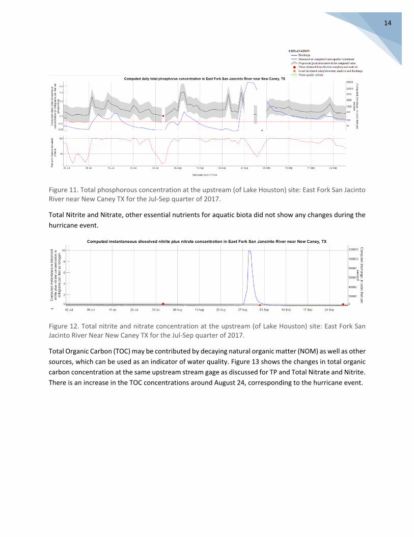
Figure 11. Total phosphorous concentration at the upstream (of Lake Houston) site: East Fork San Jacinto River near New Caney TX for the Jul-Sep quarter of 2017.
Total Nitrite and Nitrate, other essential nutrients for aquatic biota did not show any changes during the
hurricane event.
Figure 12. Total nitrite and nitrate concentration at the upstream (of Lake Houston) site: East Fork San Jacinto River Near New Caney TX for the Jul-Sep quarter of 2017.
Total Organic Carbon (TOC) may be contributed by decaying natural organic matter (NOM) as well as other
sources, which can be used as an indicator of water quality. Figure 13 shows the changes in total organic
carbon concentration at the same upstream stream gage as discussed for TP and Total Nitrate and Nitrite.
There is an increase in the TOC concentrations around August 24, corresponding to the hurricane event.

15
Figure 13. Computed daily total organic carbon concentration at the upstream (of Lake Houston) site: East Fork San Jacinto River Near New Caney TX for the Jul-Sep quarter of 2017.
Other parameters that were studied were dissolved oxygen (DO) and turbidity, obtained from the USGS-
Texas Real-Time Water Quality Information portal. DO is essential for aquatic life, with low DO values
commonly found during eutrophication, indicating poor health of the water body.9 Turbidity is an optical
indicator of suspended particulate matter in water. Turbidity may be caused by silt, fine organic or
inorganic matter matter, algae, silt or other microscopic organisms. During a storm event, particulate
matter can be transported with runoff into rivers and streams, causing higher turbidity values. High stream
velocities and discharge rates can also increase mixing and suspend sediments from the river bed. High
turbidity values can adversely affect light penetration and water quality, and may cause lakes to fill in
faster.10 Suspended sediment may also facilitate transport for other pollutants, notably metals and
bacteria, via adsorption on surface sites. Thus, turbidity values may serve as a good indicator of potential
pollution in a water body. Figure 14 shows water quality indicators at sites upstream, at the lake and
downstream of Lake Houston with associated DO and turbidity values over the period of the storm event.
While there is no clear trend for DO, the turbidity rapidly increases due to the hurricane event. As
expected, the upstream and lake site showed turbidity changes earlier (around August 27) and the
downstream site show turbidity surge around August 31, indicating the transport of the sediment and
runoff.

16
Figure 1
4. W
ater qu
ality ind
icators fo
r sites up
stream an
d d
ow
nstream
of Lake H
ou
ston
.

17
FLOOD ANALYSIS Height above nearest drainage analysis was attempted by first obtaining 1/3 arc second NED data. These
tiles were combined using Mosaic to New Raster and combined into one DEM tile. This tile was clipped to
the Basin and saved as a tiff file. Procedure from Exercise 5 was utilized to obtain the height above nearest
drainage for the basin. Processing in TauDEM took above 1.5 hours, likely due to the file size. TauDEM
only returned 3 files and did not return the ad8o file after multiple attempts. Instead, to complete the
flood analysis dataset, high water mark (HWM) data was obtained from USGS field data collection and
mapped using ArcGIS Pro. First, the Very Poor and Poor Quality data was excluded using the Definition
Query feature in the Properties tab. Next, any data that was logically inconsistent (e.g., 69 ft above
ground) was also excluded. This dataset then provides a visual representation of where inundation due to
flooding was severe. Figure 15 shows the USGS HWM data with graduated symbols for height above
ground where the HWM was found. Some regions indicated 13 ft of inundation due to the storm event.
Most of the HWMs were assessed at the south eastern regions of the basin. Buffalo Bayou and Kingwood
areas around Lake Houston were heavily flooded during the storm, which is represented well by the HWM
map showing heavy flooding in these residential and developed areas.
Figure 15. USGS HWM data represented as graduated symbols for the area under study.

18
SUMMARY AND CONCLUSIONS This study was primarily an effort to visualize the impact of a storm event like Harvey using the ArcGIS Pro
tools. First, the area of study was chosen based on high flow events and interesting surface features.
Precipitation analysis agreed with reported data for south eastern regions of the basin, showing high
precipitation totals for areas like the Buffalo Bayou-San Jacinto watershed. Spline interpolation and
Thiessen polygon method provided a qualitative and quantitative measure of the precipitation totals.
Thirdly, the water quality impacts for nutrient based contaminants did not seem to pose a higher than
usual risk to the water bodies. Turbidity increased sharply during the storm and a transport pattern can
be identified. However, this analysis was limited by available data as this was based on very few gages
around Lake Houston. Lastly, the HWM mapping provided an insight into regions that were inundated in
and around the basin. The study was able to successfully utilize geoprocessing capabilities of ArcGIS to
map several aspects of a storm event, albeit at a preliminary scale.
LIMITATIONS Availability of water quality data was a severe limitation for the term project. Height above nearest
drainage could have provided a better picture about effects at the upstream regions and how the
presence of lakes could modulate the effects of flooding by providing an equalization effect, however the
analysis remained unsuccessful at the time of submission.
FURTHER STUDY IDEAS Utilizing soil data, precipitation and some knowledge of hydrology, the study may be expanded to identify
origins of runoff to be able to identify potentially important sources of pollution during a storm event.
Time series mapping of pollutant transport can also be attempted to obtain insights on longer term effects
of a storm event.

19
REFERENCES
(1) Dottle, R.; King, R.; Koeze, E. Hurricane Harvey’s Impact - And How It Compares To Other Storms https://fivethirtyeight.com/features/hurricane-harveys-impact-and-how-it-compares-to-other-storms/ (accessed Dec 4, 2017).
(2) Griggs, B. Hurricane Harvey’s devastating impact by the numbers http://www.cnn.com/2017/08/27/us/harvey-impact-by-the-numbers-trnd/index.html (accessed Dec 4, 2017).
(3) NOAA. U.S. Billion-Dollar Weather and Climate Disasters https://www.ncdc.noaa.gov/billions/.
(4) CarnegieInstitution. Jet Streams Are Shifting And May Alter Paths Of Storms And Hurricanes https://www.sciencedaily.com/releases/2008/04/080416153558.htm (accessed Dec 5, 2017).
(5) Somashekhar, S. How Harvey went from a little-noticed storm to a behemoth https://www.washingtonpost.com/national/how-harvey-went-from-a-little-noticed-storm-to-a-behemoth/2017/08/27/2810c15a-8b5f-11e7-8df5-c2e5cf46c1e2_story.html?utm_term=.c9dd9414f188 (accessed Dec 4, 2017).
(6) Hotez, P. J.; Murray, K. O.; Buekens, P. The Gulf Coast: A New American Underbelly of Tropical Diseases and Poverty. PLoS Negl. Trop. Dis. 2014, 8 (5), 4–6.
(7) Kaplan, S.; Healy, J. Houston’s Floodwaters Are Tainted, Testing Shows https://www.nytimes.com/2017/09/11/health/houston-flood-contamination.html (accessed Dec 5, 2017).
(8) Afiune, G. Harvey’s death toll reaches 88, according to Texas health agency https://www.texastribune.org/2017/10/13/harveys-death-toll-reaches-93-people/ (accessed Dec 4, 2017).
(9) USGS. Dissolved oxygen https://water.usgs.gov/edu/dissolvedoxygen.html (accessed Dec 8, 2017).
(10) USGS. Turbidity - Water Properties https://water.usgs.gov/edu/turbidity.html (accessed Dec 8, 2017).