HURDLES FOR TURTLES: MODELING THE NESTING SUITABILITY OF LOGGERHEAD SEA TURTLES (CARETTA CARETTA) IN NORTH

CAROLINA (2005-2014)

Alyssa L. Randall Department of Geography and GeologyUniversity of North Carolina Wilmington

Advisor: Dr. Joanne Halls

Nesting ProcessFirst Emergence Body Pit Dig Egg Chamber

Oviposition Camouflage Return Crawl

ww

w.c

cctu

rtle.

org

ww

w.S

eych

elle

s-tu

rtles

.blo

gspo

t.com

ww

w.n

mlc

.org

Introduction

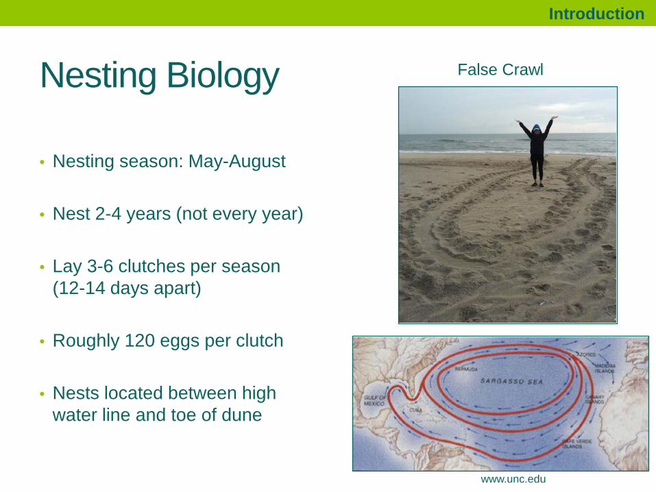
Nesting Biology

• Nesting season: May-August

• Nest 2-4 years (not every year)

• Lay 3-6 clutches per season (12-14 days apart)

• Roughly 120 eggs per clutch

• Nests located between high water line and toe of dune

Introduction

False Crawl

www.unc.edu

Critical Terrestrial Loggerhead Habitats in N.C.• NW Atlantic

Distinct Population Segment

• Northern Recovery Unit

• Designated Threatened

• 154.6 Km (96.1 miles) of critical habitat

• No management plans have been implemented at this time

Introduction

Project Significance• Very little work has been done to

merge the study of sea turtle conservation with Geographic Information Systems (GIS)

• Very few studies have used a combination of multiple variables over a large geographic area

• Results may have important implications for the designations of critical habitats and the future management of loggerhead rookeries

Introduction

(Lopez et al., 2015)

Research Questions1. Which transects within the study area are the

most prevalent for nesting?

2. What independent variables have the most statistically significant relationship with nesting locations?

3. Which statistical technique is the most useful at explaining nesting distribution?

4. Can an accurate nesting suitability predictive model be generated from independent variables?

Introduction

Independent Variables

Environmental• Elevation• Slope• Aspect• Distance to inlets• Beach width• Proximity to the Gulf

Stream (SST)

Human• Distance to hardened

structures• Beach nourishment• Housing density• Population density

Introduction

Environmental InfluencesPreference for:

• Wider (> 8.5m) beaches (Garmestani et al., 2000)

• Steeper slopes (Provancha & Erhart, 1987)

• Higher elevations (Wood & Bjorndal, 2000)

• Average sea-surface temperatures between 26°C -29°C (Coles & Musick, 2000)

Introduction

ww

w.m

arin

as.c

om

Human InfluencesPreference for:

• Low levels of artificial light (Mazor et al., 2015)

• Presence of tall buildings or dunes (Salmon et al., 1995)

• Lack of coastal armoring (Witherington et al., 2011)

• Un-nourished beaches (Long et al., 2011)

Introduction

Study Area• 515 Km (320 miles) of

potential nesting habitat

• 25 beaches

• Monitored by state and local organizations

• No monitoring at Brown’s Island (Onslow County)

Introduction

Field WorkMethodology

Data Collection, Preparation and Processing1. Created 81 beach transect polygons

• Shorelines (2004, 2009, 2012)• Digitize dune line • Digitize transect boundaries

2. Digitize oceanfront houses3. Hard structures – NCDCM4. Calculate beach width5. Import nest and false crawls

(2005-2014)

Methodology

Light Detection and Ranging (LiDAR)Methodology

• Full coverage: 2005, 2010, 2013

• Used to derive average elevation, slope, and aspect

• Ability to quickly highlight small elevational differences across the coastal landscape (Yamamota et al., 2012)

Night-time SST and Proximity to the Gulf Stream

• Query to extract the areas of water within 26°C - 29°C (May, June, July, August)

• Create polygons for these boundaries

• Calculate distance from each beach polygon to the preferred temperature polygons

Methodology

Distance to Structures and InletsCategories Inlets

1 5,000 m from inlet

2 10,000 m from inlet

3 > 10,000 m from inlet

Categories Structures

1 0

2 1-2

3 3-5

4 6-8

5 > 9

Methodology

Housing and Population DensitiesMethodology

Inverse Distance Weighted Interpolation Seasonal Housing (2010)

Beach Nourishment

• Shoreline protection and emergency beach nourishment events

• 2003-2014 to account for the gradual return of the berm to its natural state

• Comparison of the number of nests and false crawls to the occurrence of events and post-events

Methodology

http://beachnourishment.wcu.edu/

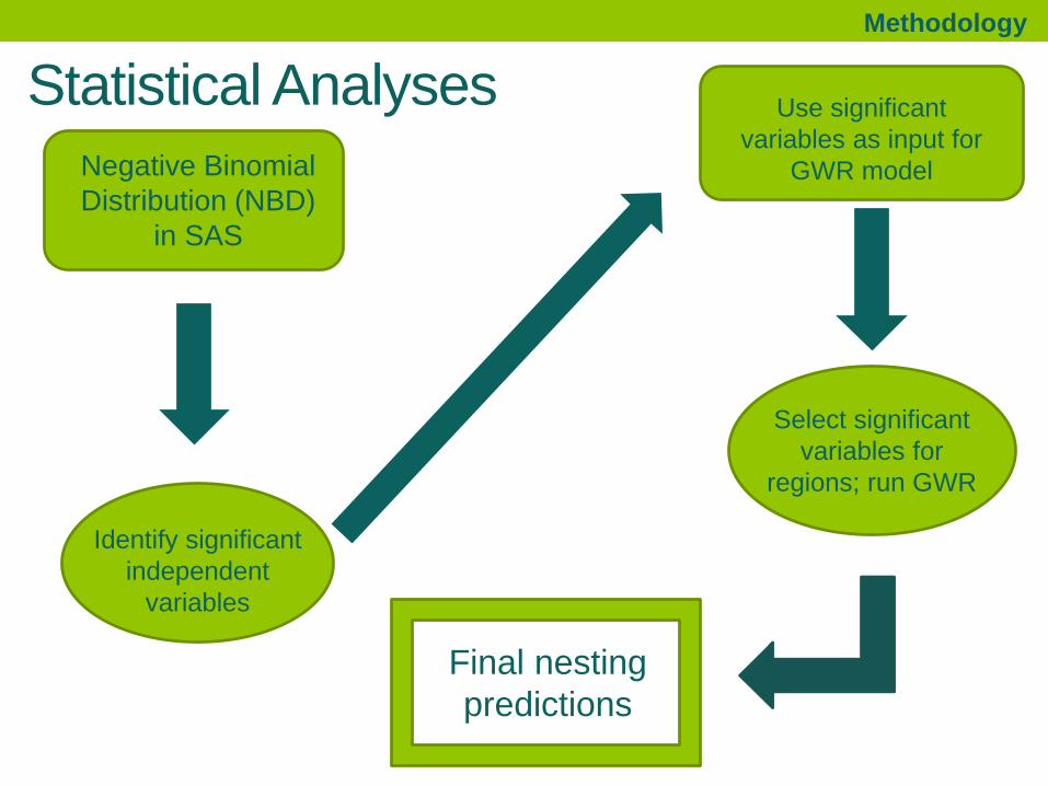
Statistical AnalysesMethodology

Negative Binomial Distribution (NBD)

in SAS

Identify significant independent

variables

Use significant variables as input for

GWR model

Select significant variables for

regions; run GWR

Final nesting predictions

Nesting/False Crawl Densities (2005-2014)

7,009 Nests 5,997 False Crawls

Results

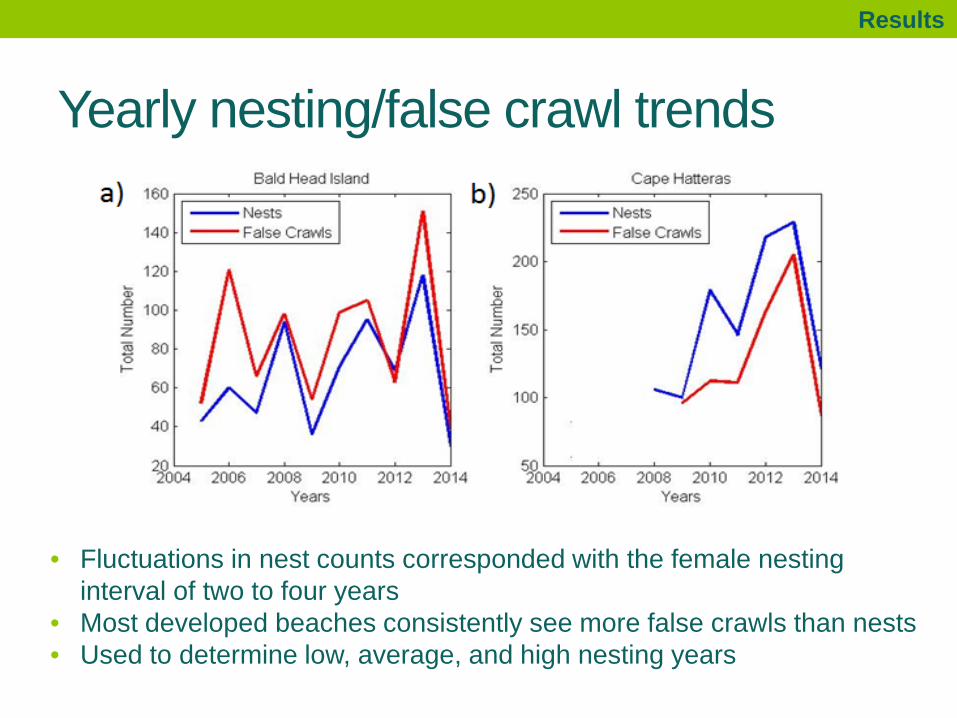
Yearly nesting/false crawl trends

Results

• Fluctuations in nest counts corresponded with the female nesting interval of two to four years

• Most developed beaches consistently see more false crawls than nests• Used to determine low, average, and high nesting years

Real-time Kinematic Elevation DataField work

SiteBeach Average Difference

(m)1 NTS 0.752 SFC 0.63 TSB N/A4 NWB -0.165 SWB 0.516 MBI 0.037 EBHI -1.978 SBHI N/A

Results

• Compared 2014 RTK elevations with 2013 LiDAR elevations

• RTK data reflected elevation patterns found in the LiDAR data

• RTK beneficial for capturing the nearshore environment when LiDAR data is unavailable

Negative Binomial Distribution Model

Positive RelationshipIndividual Variables Coupled Variables

Elevation Structure Category & Geographic RegionHouse Density & Slope

Structure Category & Inlet CategoryInverse RelationshipIndividual Variables Coupled Variables

Hard Structures House Density & ElevationNourishment Elevation & Geographic Region

Width & Geographic Region

log(𝑛𝑛𝑛𝑛𝑛𝑛𝑛𝑛 𝑐𝑐𝑐𝑐𝑐𝑐𝑛𝑛𝑛𝑛) = −1.82201 − 0.97328 ∗ 𝑆𝑆 + 0.295318 ∗ 𝑆𝑆 ∗ 𝐺𝐺 + 0.061339 ∗ 𝑆𝑆 ∗

𝐼𝐼 + 0.075497 ∗ 𝐺𝐺 ∗ 𝑌𝑌 + 0.4714 ∗ 𝐸𝐸 − 0.01704 ∗ 𝐻𝐻 ∗ 𝐸𝐸 − 0.12336 ∗ 𝐺𝐺 ∗ 𝐸𝐸 + 0.006527 ∗ 𝐻𝐻 ∗

𝑃𝑃 + 0.024062 ∗ 𝑆𝑆 ∗ 𝐼𝐼 − 0.00324 ∗ 𝐺𝐺 ∗ 𝑊𝑊 − 0.23065 ∗ 𝑁𝑁

Where: E = Elevation S = Structure Category P = Slope G = Geographic Category Y = Year Category (1 = low nesting, 2 = medium nesting, 3 = high nesting)

I = Inlet Category N = Nourishment

H = House Density W = Width

Results

Results

Environmental Variables

Results

Human Variables

Geographically Weighted Regression Model

Geographic Regions

Variables 1 2 3 4 5Structure Category 0.04159 0.52711 0.37088 0.65236 0.68728Elevation 0.85881 0.24426 0.42989 0.55894 0.86017House Density & Elevation 0.20506 0.30431 0.44286 0.58119 0.097House Density & Slope 0.53558 0.08025 0.02098 0.65224 0.76533Structure Category & Inlet Category 0.37746 0.70042 0.66109 0.6392 0.56445Slope & Inlet Category 0.72128 0.39419 0.41802 0.14075 0.59414Width 0.16035 0.05575 0.00172 0.63766 0.80199

Region Most Significant Combination of Variables R2 1 Elevation & House Density & Slope & Inlet Category 0.750012 Structure Category & Inlet Category 0.700423 Structure Category & Inlet Category 0.661094 House Density & Slope & Structure Category 0.805385 Elevation & Width 0.83459

Results

Results

Overall, the GWR model performed best for all years

(2005-2014)

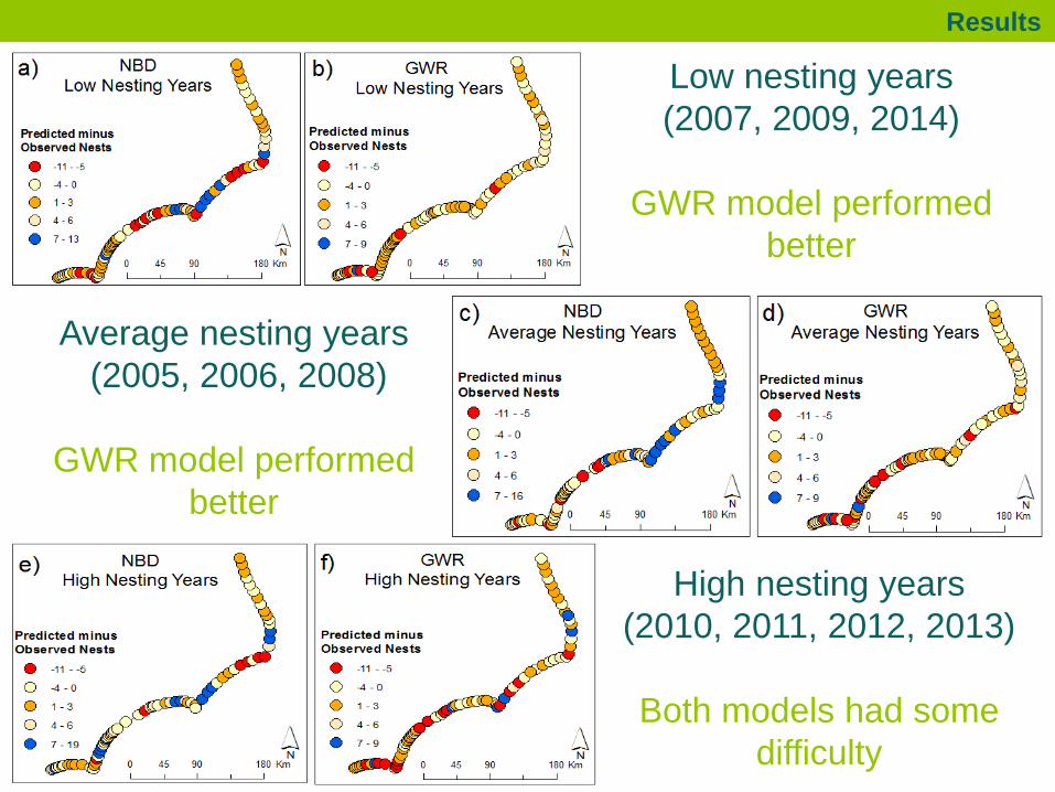
Low nesting years (2007, 2009, 2014)

GWR model performed better

Average nesting years(2005, 2006, 2008)

GWR model performed better

High nesting years (2010, 2011, 2012, 2013)

Both models had some difficulty

Results

Final Prediction of Nesting DensitiesResults

Elevation, House Density, Slope, Inlets

Structures, Inlets

Structures, Inlets

House Density, Slope,

StructuresElevation,

Width

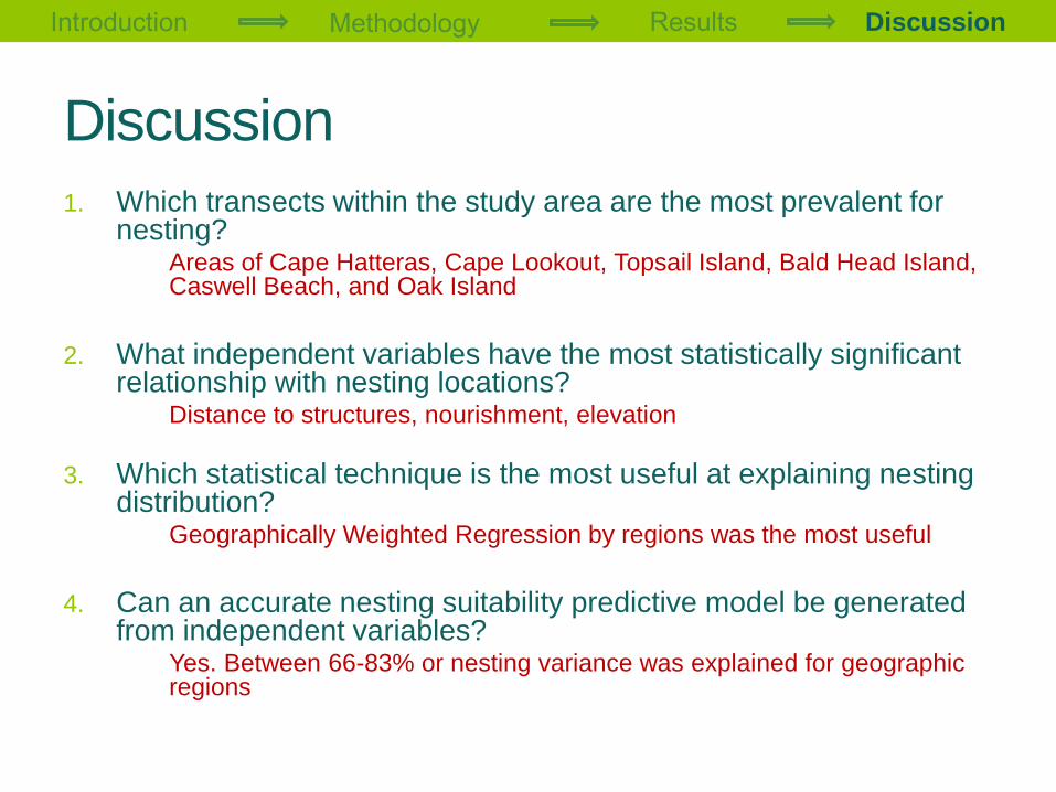
Discussion1. Which transects within the study area are the most prevalent for

nesting?Areas of Cape Hatteras, Cape Lookout, Topsail Island, Bald Head Island, Caswell Beach, and Oak Island

2. What independent variables have the most statistically significant relationship with nesting locations?

Distance to structures, nourishment, elevation

3. Which statistical technique is the most useful at explaining nesting distribution?

Geographically Weighted Regression by regions was the most useful

4. Can an accurate nesting suitability predictive model be generated from independent variables?

Yes. Between 66-83% or nesting variance was explained for geographic regions

Discussion

Contributions• Possible to develop predictive geographic model that covers a

large area

• Similar findings: higher elevations favorable (Wood & Bjorndal, 2000), width is significant (Garmestani et al., 2000), hard structures can affect nesting (Witherington et al., 2011), nourishment can deter nesting (Brock et al., 2009)

• Use of LiDAR highly recommended for future studies

• Different factors found significant in the distinct regions

• Using the NBD and GWR model in conjunction, by geographic region, is the most successful method for modeling nesting trends (2005-2014)

Discussion

Recommendations • Accurate and consistent nesting data

• Improved GPS technology for recording nest/false crawl sites

• Access to dredging/nourishment final reports

Discussion

ww

w.w

itn.c

om

Future Work• Revisit transects that did not fit the model well

• Predictive equations for each beach

• Policy implementations: hard structures,nourishment, artificial light ordinances

Discussion