Human Embryonic Stem Cell Detection by Spatial Informationand Mixture of Gaussians

Benjamin Xueqi Guan, Bir Bhanu, Ninad ThakoorElectrical Engineering

University of California, RiversideRiverside, USA

Email: {xguan001, bhanu, nthakoor}@ee.ucr.edu

Prudence Talbot, Sabrina LinCell Biology and Neuroscience

University of California, RiversideRiverside, USA

Email: {prudence.talbot, sabrina.lin}@ucr.edu

Abstract—Human Embryonic Stem Cells (HESCs) possessthe potential to provide treatments for cancer, Parkinson’sdisease, Huntington’s disease, Type 1 diabetes mellitus etc. Con-sequently, HESCs are often used in the biological assay to studythe effects of chemical agents in the human body. However,detection of HESC is often a challenge in phase contrast images.To improve the accuracy of HESC colony detection, we combinespatial information and the outcome of a mixture of Gaussiansmodel. While a mixture of Gaussians generates reasonablelabels for various regions of HESC images, it lacks spatialdetails and connectivity. Sets of spatially consistent candidatelabeling are generated by median filtering the image at differentscales followed by thresholding. An optimal combination offilter scale and threshold which maximizes the correlationcoefficient between the spatial information and the mixture ofGaussians output is obtained. The paper validates the methodfor various HESC videos.

Keywords- Apoptosis, Cell Detection, Human EmbryonicStem Cell, Expectation-Maximization Algorithm, Mixture ofGaussians, Spatial Information.

I. INTRODUCTION

Biologists often use noninvasive microscopy imagingtechnique such as phase contrast imaging to study livingbiological specimens and to learn about their behavior [1].This paper focuses on Human Embryonic Stem Cell (HESC)phase contrast images taken from the BioStation IM [2].The HESC has the capacity to differentiate into diversehuman cell types. With the aforementioned characteristic,it is well known that HESCs have the potential to be usedin cell replacement therapies for the treatment of humandiseases [3]. Subsequently, biologists need to study theHESCs more closely under different chemical conditionsin large data sets. However, the study of large volume ofdata is strenuous and laborious for a human. Therefore,biologists need a good tracking technique to understand thebehavior of the stem cells over time. Towards developing anautomated stem cell tracking system, cell detection plays animportant role. However, there are a number of challengesthat make the cell detection challenging: (1) the low signal-to-noise ratio of the phase contrast microscopy images; (2)the topological complexity of cell shapes; and (3) the low

(a) (b)

(c) (d)

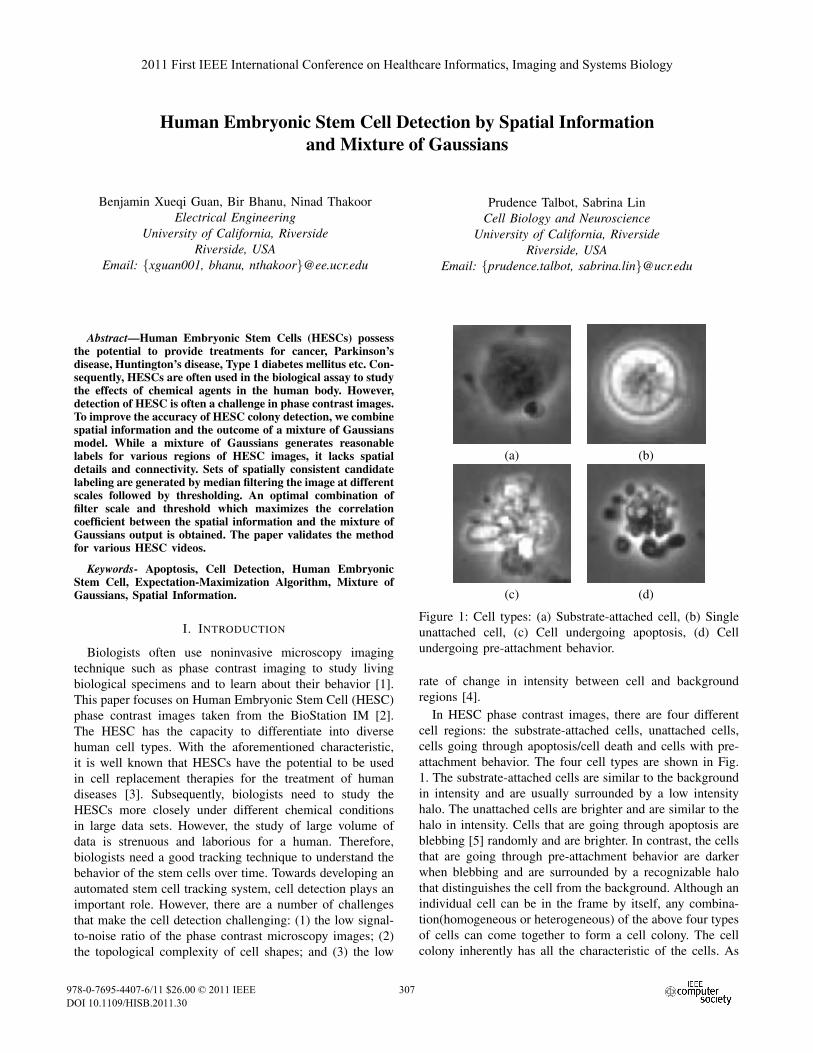
Figure 1: Cell types: (a) Substrate-attached cell, (b) Singleunattached cell, (c) Cell undergoing apoptosis, (d) Cellundergoing pre-attachment behavior.

rate of change in intensity between cell and backgroundregions [4].

In HESC phase contrast images, there are four differentcell regions: the substrate-attached cells, unattached cells,cells going through apoptosis/cell death and cells with pre-attachment behavior. The four cell types are shown in Fig.1. The substrate-attached cells are similar to the backgroundin intensity and are usually surrounded by a low intensityhalo. The unattached cells are brighter and are similar to thehalo in intensity. Cells that are going through apoptosis areblebbing [5] randomly and are brighter. In contrast, the cellsthat are going through pre-attachment behavior are darkerwhen blebbing and are surrounded by a recognizable halothat distinguishes the cell from the background. Although anindividual cell can be in the frame by itself, any combina-tion(homogeneous or heterogeneous) of the above four typesof cells can come together to form a cell colony. The cellcolony inherently has all the characteristic of the cells. As

2011 First IEEE International Conference on Healthcare Informatics, Imaging and Systems Biology

978-0-7695-4407-6/11 $26.00 © 2011 IEEE

DOI 10.1109/HISB.2011.30

111

2011 First IEEE International Conference on Healthcare Informatics, Imaging and Systems Biology

978-0-7695-4407-6/11 $26.00 © 2011 IEEE

DOI 10.1109/HISB.2011.30

307

2011 First IEEE International Conference on Healthcare Informatics, Imaging and Systems Biology

978-0-7695-4407-6/11 $26.00 © 2011 IEEE

DOI 10.1109/HISB.2011.30

307

seen in Fig. 1(a), the detection for substrate-attached cellsand cell colonies that consist of substrate-attached cells isharder than the detection for other type of cells and cellcolonies. As a result, a method for accurate detection ofsubstrate-attached cells or colony that consist of substrate-attached cells is needed. In this paper, a combination of spa-tial information and a mixture of Gaussians, which improvesdetection accuracy of the cell regions, is introduced.

II. RELATED WORK AND CONTRIBUTIONS

Previous works have shown approaches for cell regiondetection in phase contrast images [4], [6]. Ambriz-Colinet al. [6] discuss two methods for cell region detection:detection by pixels intensity variance (PIV) and by graylevel morphological gradient (GLMG). The PIV methodperforms pixel classification on the normalized image. Itrecognizes the probable cell regions and labels the rest as thebackground in the normalized image. The GLMG methoddetects the cell regions by using morphological gradient thatis calculated from the dilation and erosion operations, and bya threshold that separates the pixels belonging to a cell andto the background. Li et al. [4] also mention a combineduse of morphological rolling-ball filtering and a BayesianClassifier that is based on the estimated cell and backgroundgray scale histograms to classify the image pixels into eitherthe cell regions or the background.

We suggest using spatial information and the result fromthe mixture of Gaussians model to estimate the cell regions.The mixture of Gaussians provides an estimate for variouscell regions. However, it lacks spatial consistency as the cellregion intensities lie on both lower and higher side of thebackground intensities. We generate spatial information forthe image first. The result from the mixture of Gaussians isthen used to estimate the optimal threshold to segment thespatial information into cell regions and background.

III. TECHNICAL APPROACH

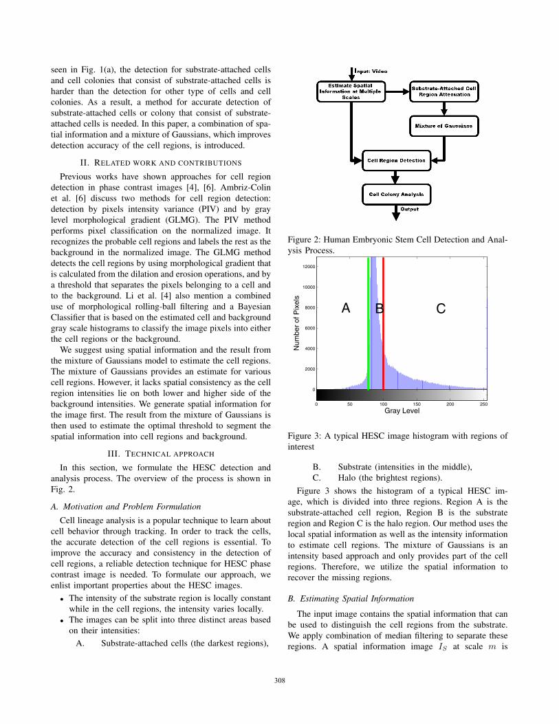
In this section, we formulate the HESC detection andanalysis process. The overview of the process is shown inFig. 2.

A. Motivation and Problem Formulation

Cell lineage analysis is a popular technique to learn aboutcell behavior through tracking. In order to track the cells,the accurate detection of the cell regions is essential. Toimprove the accuracy and consistency in the detection ofcell regions, a reliable detection technique for HESC phasecontrast image is needed. To formulate our approach, weenlist important properties about the HESC images.

∙ The intensity of the substrate region is locally constantwhile in the cell regions, the intensity varies locally.

∙ The images can be split into three distinct areas basedon their intensities:

A. Substrate-attached cells (the darkest regions),

Figure 2: Human Embryonic Stem Cell Detection and Anal-ysis Process.

0

2000

4000

6000

8000

10000

12000

Num

ber

of P

ixel

s

Gray Levels

Gray Level0 50 100 150 200 250

B CA

Figure 3: A typical HESC image histogram with regions ofinterest

B. Substrate (intensities in the middle),C. Halo (the brightest regions).

Figure 3 shows the histogram of a typical HESC im-age, which is divided into three regions. Region A is thesubstrate-attached cell region, Region B is the substrateregion and Region C is the halo region. Our method uses thelocal spatial information as well as the intensity informationto estimate cell regions. The mixture of Gaussians is anintensity based approach and only provides part of the cellregions. Therefore, we utilize the spatial information torecover the missing regions.

B. Estimating Spatial Information

The input image contains the spatial information that canbe used to distinguish the cell regions from the substrate.We apply combination of median filtering to separate theseregions. A spatial information image 𝐼𝑆 at scale 𝑚 is

112308308

estimated as,

𝐼𝑆(𝑚) = 𝑚𝑒𝑑(𝑎𝑏𝑠(𝐼 −𝑚𝑒𝑑(𝐼,𝑚)),𝑚+ 2) (1)

where 𝑚𝑒𝑑(⋅, 𝑠) denotes the median filtering operation withwindow size 𝑠 and 𝐼 is the original image. The operation𝑎𝑏𝑠(𝐼 − 𝑚𝑒𝑑(𝐼,𝑚)) yields low values in the area withconstant local intensity (i.e., substrate) and high values inareas with varying intensities (i.e. cell regions). The largermedian filter smooths interior cell regions while preserv-ing the edges. Unlike the original image which has threeintensity modes, the spatial information image is bimodal.Thus, a single threshold can be used to separate the substrateand cell regions. However, one still has to select appropriatethreshold 𝑇 and scale 𝑚.

With the estimated spatial information, 𝐼𝑆 from equa-tion (1), we can choose the spatial information with aspecific window size to selectively attenuate the input imagefor the mixture of Gaussians which follows. We normalizethe spatial information at location (𝑟, 𝑐) as,

𝐼𝑀𝑆(𝑟, 𝑐) = 1− 𝐼𝑆(𝑟, 𝑐)

max(𝐼𝑆)(2)

𝐼𝑀𝑆 is then used to attenuate the original image:

𝐼𝐺(𝑟, 𝑐) = 𝐼(𝑟, 𝑐)× 𝐼𝑀𝑆(𝑟, 𝑐) (3)

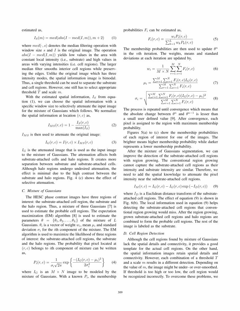
𝐼𝐺 is the attenuated image that is used as the input imageto the mixture of Gaussians. The attenuation affects bothsubstrate-attached cells and halo regions. It creates moreseparation between substrate and substrate-attached cells.Although halo regions undergo undesired attenuation, theeffect is minimal due to the high contrast between thesubstrate and halo regions. Fig. 4 (c) shows the effect ofselective attenuation.

C. Mixture of Gaussians

The HESC phase contrast images have three regions ofinterest: the substrate-attached cell region, the substrate andthe halo region. Thus, a mixture of three Gaussians [7] isused to estimate the probable cell regions. The expectationmaximization (EM) algorithm [8] is used to estimate theparameters 𝜃 = {𝜃1, 𝜃2, . . . , 𝜃𝐿} of the mixture of 𝐿Gaussians. 𝜃𝑖 is a vector of weight 𝑤𝑖, mean 𝜇𝑖 and standarddeviation 𝜎𝑖 for the 𝑖th component of the mixture. The EMalgorithm is used to maximize the likelihood of three regionsof interest: the substrate-attached cell regions, the substrateand the halo regions. The probability that pixel located at(𝑟, 𝑐) belongs to 𝑖th component of mixture can be writtenas,

𝑃𝑖(𝑟, 𝑐) =1

𝜎𝑖

√2𝜋

exp

{−(𝐼𝐺(𝑟, 𝑐)− 𝜇𝑖)2

2𝜎2𝑖

}(4)

where 𝐼𝐺 is an 𝑀 × 𝑁 image to be modeled by themixture of Gaussians. With a known 𝑃𝑖, the membership

probabilities 𝐹𝑖 can be estimated as,

𝐹𝑖(𝑟, 𝑐) =𝑤𝑖𝑃𝑖(𝑟, 𝑐)∑𝐿

𝑘=1 𝑤𝑘𝑃𝑘(𝑟, 𝑐)(5)

The membership probabilities are then used to update 𝜃𝑛

in the 𝑛th iteration. The weights, means and standarddeviations at each iteration are updated by,

𝑤𝑖 =1

𝑀 ×𝑁

𝑀∑𝑟=1

𝑁∑𝑐=1

𝐹𝑖(𝑟, 𝑐) (6)

𝜇𝑖 =

∑𝑀𝑟=1

∑𝑁𝑐=1 𝐹𝑖(𝑟, 𝑐)𝐼𝐺(𝑟, 𝑐)∑𝑀

𝑟=1

∑𝑁𝑐=1 𝐹𝑖(𝑟, 𝑐)

(7)

𝜎𝑖 =

√√√⎷∑𝑀𝑟=1

∑𝑁𝑐=1 𝐹𝑖(𝑟, 𝑐)(𝐼𝐺(𝑟, 𝑐)− 𝜇𝑖)2∑𝑀𝑟=1

∑𝑁𝑐=1 𝐹𝑖(𝑟, 𝑐)

(8)

The process is repeated until convergence which means thatthe absolute change between 𝜃𝑛 and 𝜃𝑛−1 is lesser thana small user defined value [9]. After convergence, eachpixel is assigned to the region with maximum membershipprobability.

Figures 5(a) to (c) show the membership probabilitiesof each region of interest for one of the images. Thebrighter means higher membership probability while darkerrepresents a lower membership probability.

After the mixture of Gaussians segmentation, we canimprove the detection of the substrate-attached cell regionswith region growing. The conventional region growingcannot capture the substrate-attached cell regions as theirintensity and substrate intensity are similar. Therefore, weneed to add the spatial knowledge to attenuate the pixelintensity near the substrate-attached cell regions.

𝐼𝑀 (𝑟, 𝑐) = 𝐼𝐺(𝑟, 𝑐)− 𝐼𝐺(𝑟, 𝑐) exp (−𝐼𝐷(𝑟, 𝑐)) (9)

where 𝐼𝐷 is a Euclidean distance transform of the substrate-attached cell regions. The effect of equation (9) is shown inFig. 6(b). The local information used in equation (9) helpsdetecting the substrate-attached cell regions that conven-tional region growing would miss. After the region growing,grown substrate-attached cell regions and halo regions arecombined to form the probable cell regions. The rest of theimage is labeled as the substrate.

D. Cell Region Detection

Although the cell regions found by mixture of Gaussianslack the spatial details and connectivity, it provides a goodtemplate for the actual cell regions. On the other hand,the spatial information images retain spatial details andconnectivity. However, each combination of a threshold 𝑇and a scale 𝑚 results in a different detection. Depending onthe value of 𝑚, the image might be under- or over-smoothed.If threshold is too high or too low, the cell region wouldbe recognized incorrectly. To overcome these problems, we

113309309

(a) (b) (c)

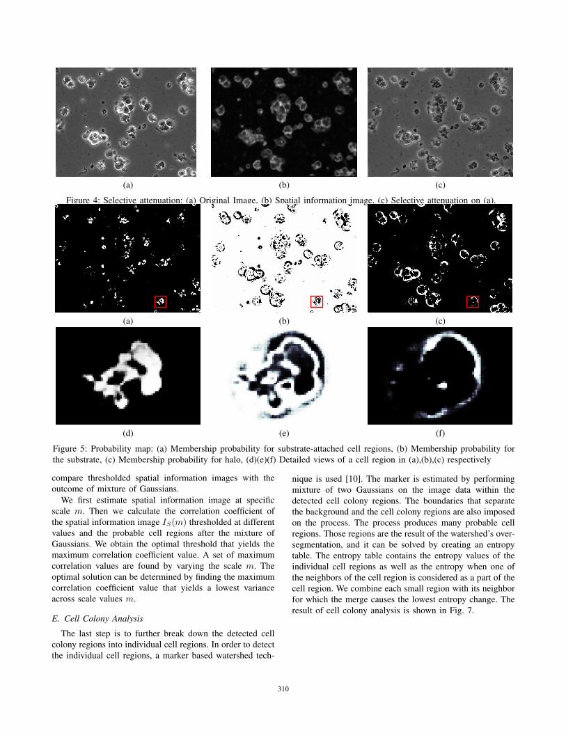
Figure 4: Selective attenuation: (a) Original Image, (b) Spatial information image, (c) Selective attenuation on (a).

(a) (b) (c)

(d) (e) (f)

Figure 5: Probability map: (a) Membership probability for substrate-attached cell regions, (b) Membership probability forthe substrate, (c) Membership probability for halo, (d)(e)(f) Detailed views of a cell region in (a),(b),(c) respectively

compare thresholded spatial information images with theoutcome of mixture of Gaussians.

We first estimate spatial information image at specificscale 𝑚. Then we calculate the correlation coefficient ofthe spatial information image 𝐼𝑆(𝑚) thresholded at differentvalues and the probable cell regions after the mixture ofGaussians. We obtain the optimal threshold that yields themaximum correlation coefficient value. A set of maximumcorrelation values are found by varying the scale 𝑚. Theoptimal solution can be determined by finding the maximumcorrelation coefficient value that yields a lowest varianceacross scale values 𝑚.

E. Cell Colony Analysis

The last step is to further break down the detected cellcolony regions into individual cell regions. In order to detectthe individual cell regions, a marker based watershed tech-

nique is used [10]. The marker is estimated by performingmixture of two Gaussians on the image data within thedetected cell colony regions. The boundaries that separatethe background and the cell colony regions are also imposedon the process. The process produces many probable cellregions. Those regions are the result of the watershed’s over-segmentation, and it can be solved by creating an entropytable. The entropy table contains the entropy values of theindividual cell regions as well as the entropy when one ofthe neighbors of the cell region is considered as a part of thecell region. We combine each small region with its neighborfor which the merge causes the lowest entropy change. Theresult of cell colony analysis is shown in Fig. 7.

114310310

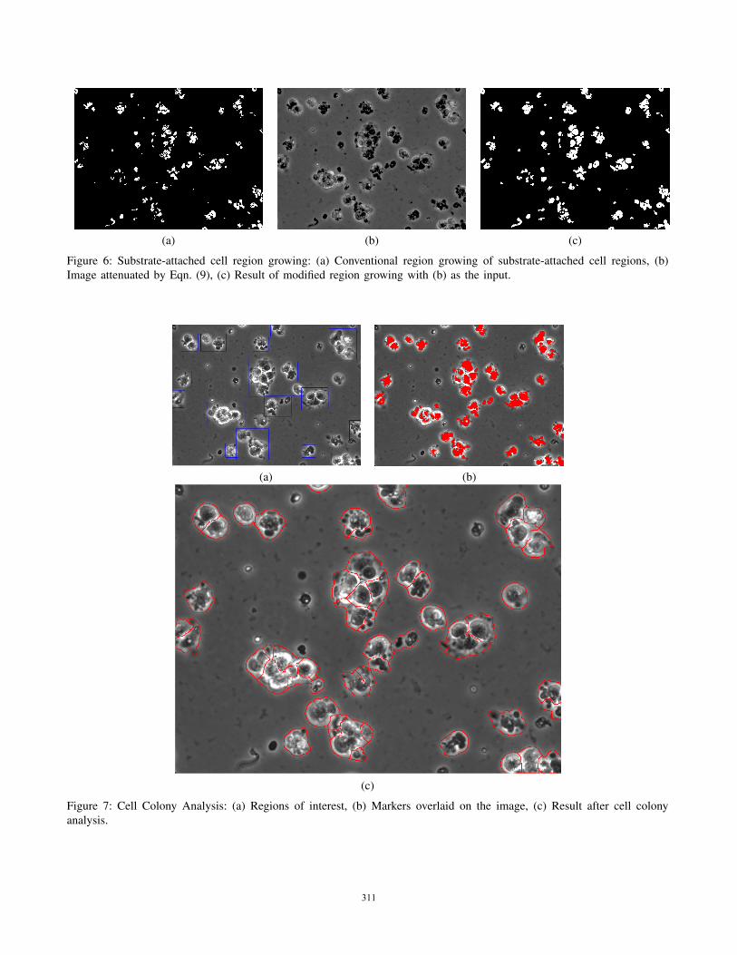
(a) (b) (c)

Figure 6: Substrate-attached cell region growing: (a) Conventional region growing of substrate-attached cell regions, (b)Image attenuated by Eqn. (9), (c) Result of modified region growing with (b) as the input.

(a) (b)

(c)

Figure 7: Cell Colony Analysis: (a) Regions of interest, (b) Markers overlaid on the image, (c) Result after cell colonyanalysis.

115311311

IV. EXPERIMENTAL RESULTS

A. Data

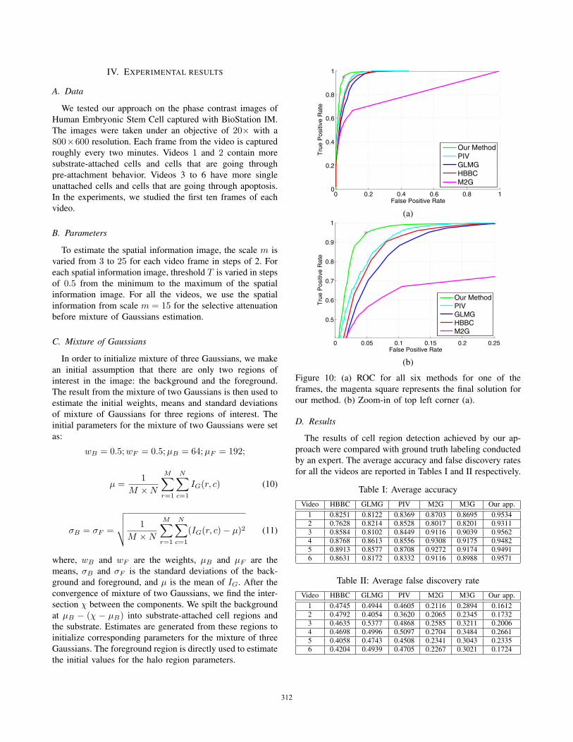
We tested our approach on the phase contrast images ofHuman Embryonic Stem Cell captured with BioStation IM.The images were taken under an objective of 20× with a800×600 resolution. Each frame from the video is capturedroughly every two minutes. Videos 1 and 2 contain moresubstrate-attached cells and cells that are going throughpre-attachment behavior. Videos 3 to 6 have more singleunattached cells and cells that are going through apoptosis.In the experiments, we studied the first ten frames of eachvideo.

B. Parameters

To estimate the spatial information image, the scale 𝑚 isvaried from 3 to 25 for each video frame in steps of 2. Foreach spatial information image, threshold 𝑇 is varied in stepsof 0.5 from the minimum to the maximum of the spatialinformation image. For all the videos, we use the spatialinformation from scale 𝑚 = 15 for the selective attenuationbefore mixture of Gaussians estimation.

C. Mixture of Gaussians

In order to initialize mixture of three Gaussians, we makean initial assumption that there are only two regions ofinterest in the image: the background and the foreground.The result from the mixture of two Gaussians is then used toestimate the initial weights, means and standard deviationsof mixture of Gaussians for three regions of interest. Theinitial parameters for the mixture of two Gaussians were setas:

𝑤𝐵 = 0.5;𝑤𝐹 = 0.5;𝜇𝐵 = 64;𝜇𝐹 = 192;

𝜇 =1

𝑀 ×𝑁

𝑀∑𝑟=1

𝑁∑𝑐=1

𝐼𝐺(𝑟, 𝑐) (10)

𝜎𝐵 = 𝜎𝐹 =

√√√⎷ 1

𝑀 ×𝑁

𝑀∑𝑟=1

𝑁∑𝑐=1

(𝐼𝐺(𝑟, 𝑐)− 𝜇)2 (11)

where, 𝑤𝐵 and 𝑤𝐹 are the weights, 𝜇𝐵 and 𝜇𝐹 are themeans, 𝜎𝐵 and 𝜎𝐹 is the standard deviations of the back-ground and foreground, and 𝜇 is the mean of 𝐼𝐺. After theconvergence of mixture of two Gaussians, we find the inter-section 𝜒 between the components. We spilt the backgroundat 𝜇𝐵 − (𝜒 − 𝜇𝐵) into substrate-attached cell regions andthe substrate. Estimates are generated from these regions toinitialize corresponding parameters for the mixture of threeGaussians. The foreground region is directly used to estimatethe initial values for the halo region parameters.

0 0.2 0.4 0.6 0.8 10

0.2

0.4

0.6

0.8

1

False Positive Rate

Tru

e P

ositi

ve R

ate

Our MethodPIVGLMGHBBCM2G

(a)

0 0.05 0.1 0.15 0.2 0.25

0.5

0.6

0.7

0.8

0.9

1

False Positive Rate

Tru

e P

ositi

ve R

ate

Our MethodPIVGLMGHBBCM2G

(b)

Figure 10: (a) ROC for all six methods for one of theframes, the magenta square represents the final solution forour method. (b) Zoom-in of top left corner (a).

D. Results

The results of cell region detection achieved by our ap-proach were compared with ground truth labeling conductedby an expert. The average accuracy and false discovery ratesfor all the videos are reported in Tables I and II respectively.

Table I: Average accuracy

Video HBBC GLMG PIV M2G M3G Our app.

1 0.8251 0.8122 0.8369 0.8703 0.8695 0.95342 0.7628 0.8214 0.8528 0.8017 0.8201 0.93113 0.8584 0.8102 0.8449 0.9116 0.9039 0.95624 0.8768 0.8613 0.8556 0.9308 0.9175 0.94825 0.8913 0.8577 0.8708 0.9272 0.9174 0.94916 0.8631 0.8172 0.8332 0.9116 0.8988 0.9571

Table II: Average false discovery rate

Video HBBC GLMG PIV M2G M3G Our app.

1 0.4745 0.4944 0.4605 0.2116 0.2894 0.16122 0.4792 0.4054 0.3620 0.2065 0.2345 0.17323 0.4635 0.5377 0.4868 0.2585 0.3211 0.20064 0.4698 0.4996 0.5097 0.2704 0.3484 0.26615 0.4058 0.4743 0.4508 0.2341 0.3043 0.23356 0.4204 0.4939 0.4705 0.2267 0.3021 0.1724

116312312

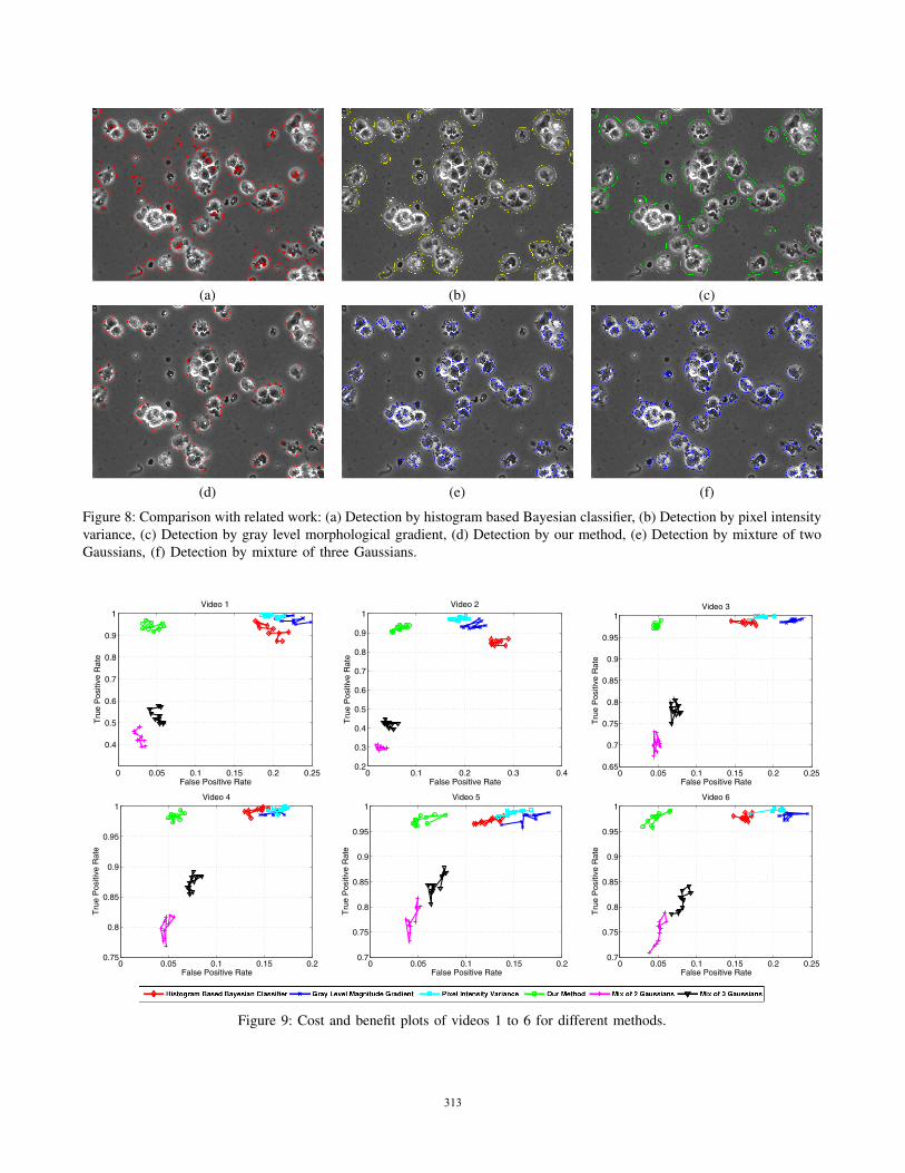
(a) (b) (c)

(d) (e) (f)

Figure 8: Comparison with related work: (a) Detection by histogram based Bayesian classifier, (b) Detection by pixel intensityvariance, (c) Detection by gray level morphological gradient, (d) Detection by our method, (e) Detection by mixture of twoGaussians, (f) Detection by mixture of three Gaussians.

0 0.05 0.1 0.15 0.2 0.25

0.4

0.5

0.6

0.7

0.8

0.9

1

False Positive Rate

Tru

e P

ositi

ve R

ate

Video 1

0 0.1 0.2 0.3 0.40.2

0.3

0.4

0.5

0.6

0.7

0.8

0.9

1

False Positive Rate

Tru

e P

ositi

ve R

ate

Video 2

0 0.05 0.1 0.15 0.2 0.250.65

0.7

0.75

0.8

0.85

0.9

0.95

1

False Positive Rate

Tru

e P

ositi

ve R

ate

Video 3

0 0.05 0.1 0.15 0.20.75

0.8

0.85

0.9

0.95

1

False Positive Rate

Tru

e P

ositi

ve R

ate

Video 4

0 0.05 0.1 0.15 0.20.7

0.75

0.8

0.85

0.9

0.95

1

False Positive Rate

Tru

e P

ositi

ve R

ate

Video 5

0 0.05 0.1 0.15 0.2 0.250.7

0.75

0.8

0.85

0.9

0.95

1

False Positive Rate

Tru

e P

ositi

ve R

ate

Video 6

Figure 9: Cost and benefit plots of videos 1 to 6 for different methods.

117313313

1 2 3 4 5 6 7 8 9 100

10

20

30

40

50

60

70

Frame #

Num

ber

of C

ells

Ground TruthEstimated Cell Count

Figure 11: Comparison of estimated cell counts with theactual cell counts for video 1.

For comparison, we implemented PIV, GLMG and his-togram based Bayesian classifier (HBBC) detection meth-ods. The result of our method and these methods are shownin Figs. 8(a) to (d). We can see that the overestimation ofcell regions is a major problem for the PIV, GLMG andHBBC methods. Moreover, detection by PIV and GLMGrequire a user defined threshold to determine whether a pixelbelongs to the cell region or to the substrate. The HBBCmethod is more tedious compared to other methods since itrequires ground truth for the cell regions for training of theclassifier. Our method needs only an initial scale to estimatethe spatial information image for selective attenuation anda largest allowable scale that is to be used for optimization.In addition, we compare our approach with the outcomefrom the mixture of two and three Gaussians as shown inFigs. 8(e) and (f) respectively. The performance of all thesix methods is summarized in Tables I and II. Table II showsthat our method has a consistent low false discovery rate.The low false discovery rate for mixture of Gaussians isdue to the underestimation of cell regions by the method.Table I shows that our approach yields higher accuracy incell region detections compared to other methods. The cost(False positives) and benefit (True positives) statistics for allsix videos is shown in Fig. 9. As one can see, our methodhas a high true positive rate while maintaining a low falsepositive rate for all six videos. Figures 10(a) and (b) showthe ROC plots for all the methods discussed in this paper andour method outperforms all other methods. Figure 11 showsthe cell count results compared to the cell count groundtruth. Although the cell counts are satisfactory, the currentmethod overestimates the count.

V. CONCLUSIONS

In this paper, we proposed a cell region detection methodby using spatial information and mixture of Gaussiansmodel. This method gives tight boundaries for cell regions.The method can be used for individual cell detection with

the local markers found by the mixture of Gaussians. Ex-periments were carried out to test the method for cell regiondetection and the results show that it provides a betterdetection accuracy than the other methods in literature. Inthe future, our work will focus on further improving thecell colony analysis by developing a new marker detectionmethod. We will also look into developing a tracking systemfor the HESCs.

ACKNOWLEDGMENT

This work is supported by the NSF Integrated GraduateEducation Research and Training (IGERT): Video Bioinfor-matics Grant DGE 0903667.

REFERENCES

[1] R. Yu, M. Wu, S. Lin, and P. Talbot, “Cigarette SmokeToxicants Alter Growth and Survival of Cultured MammalianCells,” Toxicological Sciences, vol. 93, no. 1, pp. 82–95, 2006.

[2] Biostation-IM. [Online]. Available:http://www.nikoninstruments.com/Vyrobky/Cell-Incubator-Observation/BioStation-IM

[3] M. Stojkovic, M. Lako, T. Strachan, and A. Murdoch,“Derivation, growth and applications of human embryonicstem cells,” Reproduction, vol. 128, no. 3, pp. 259–267, 2004.

[4] K. Li, M. Chen, and T. Kanade, “Cell population trackingand lineage construction with spatiotemporal context,” inProceedings of the 10th International Conference on Med-ical Image Computing and Computer-Assisted Intervention(MICCAI), 2007, pp. 295 – 302.

[5] O. Fackler and R. Grosse, “Cell motility through plasmamembrane blebbing,” J Cell Biol., vol. 181, no. 6, p. 879884,2008.

[6] F. Ambriz-Colin, M. Torres-Cisneros, J. Avina-Cervantes,J. Saavedra-Martinez, O. Debeir, and J. Sanchez-Mondragon,“Detection of biological cells in phase-contrast microscopyimages,” in Artificial Intelligence, 2006. MICAI ’06. FifthMexican International Conference on, 2006, pp. 68 –77.

[7] D. A. Forsyth and J. Ponce, Computer Vision: A ModernApproach. Prentice Hall Professional Technical Reference,2002.

[8] A. P. Dempster, N. M. Laird, and D. B. Rubin, “Maximumlikelihood from incomplete data via the EM algorithm,” Jour-nal of the Royal Statistical Society. Series B (Methodological),vol. 39, no. 1, pp. pp. 1–38, 1977.

[9] S. Gopinath, Q. Wen, N. Thakoor, K. Luby-Phelps, and J. X.Gao, “A statistical approach for intensity loss compensationof confocal microscopy images,” Journal of Microscopy, vol.230, no. 1, pp. 143–159, 2008.

[10] F. Cloppet and A. Boucher, “Segmentation of complex nu-cleus configurations in biological images,” Pattern Recogn.Lett., vol. 31, pp. 755–761, June 2010.

118314314