20g%20-%20lake%20meredith%20study

APPENDIX G

HISTORICAL TRENDS IN KEY COMPONENTS

OF THE HYDROLOGIC CYCLE FOR THE

LAKE MERIDETH WATERSHED

TO: File – PPC07480 FROM: Spencer Schnier and Andres Salazar SUBJECT: Historical Trends in Key Components of the Hydrologic Cycle for the Lake

Meredith Watershed DATE: July 27, 2010

1.0. INTRODUCTION Lake Meredith is located in the Texas Panhandle (Figure 1) and is a significant water

supply for the Panhandle Water Planning Area (PWPA). Sanford Dam was constructed in 1965 impounding the Canadian River to form Lake Meredith. The reservoir had an intended capacity of nearly 864,400 ac-ft (as modeled in Run 3 of the Canadian WAM), but has only reached maximum of 60% full during a period in the 1970s (Figure 2). Precipitous declines in content have been observed since 2000. The streamflows that fill Lake Meredith have trended substantially downwards over the past 70 years, with flows from the last decade being especially low (Figure 3).

Currently, the lake is at a historic low content of 27,000 ac-ft (less than 4% of the original capacity). The reliable supply from Lake Meredith has decreased from over 70,000 acre-feet per year to about 30,000 acre-feet per year in 2008. The impact of the reduced supplies to the PWPA is great. Without renewable surface water, the region must rely on groundwater.

This study was conducted to better understand the current decline in Lake Meredith water supplies and assess whether this supply reduction is transient or a long-term trend. Other regional surface water sources, Lake Palo Duro and Lake Greenbelt, are also in drought conditions. The Lake Meredith study could have important implications for these reservoirs as well. The study evaluated several potential causes of reduced inflows, including hydrologic loss, groundwater-surface water interactions and changes in land use.

FINAL REPORT

Historical Trends in Key Components of the Hydrologic Cycle for the Lake Meredith Watershed 7/27/2010 Page 2 of 72

Figure 1. Map of the Lake Meredith Watershed


Figure 2. Historical Storage Levels in Lake Meredith


Figure 3. Historical Streamflows at the Amarillo Gage (07227500) near Lake Meredith

The Lake Meredith study is organized into six sections. The first section introduces the

issue and provides background information describing the problem. Section 2 documents the

calculation of hydrologic loss by decade and evaluates trends in the rainfall to runoff ratio.

Section 3 analyzes trends in temperature and precipitation. Section 4 examines interactions

between groundwater and surface water as a possible cause for declining lake levels. Section 5

investigates whether changing land use practices are reducing the watershed’s ability to generate

runoff. Finally, section 6 presents a summary of the findings and the conclusions of the research.

2.0. Hydrologic Loss

In this study, the net hydrologic loss is defined as the amount of precipitation that does

not contribute to increased runoff at the outlet of the watershed. Historical changes to hydrologic

loss were evaluated for the Canadian River watershed between Logan and Amarillo. Hydrologic

loss can occur due to evaporation, transpiration, and/or infiltration. It is indicative of the

watershed’s ability to generate runoff from precipitation events.

10

100

1,000

10,000

1939

1942

1945

1948

1951

1954

1957

1960

1963

1966

1969

1972

1975

1978

1981

1984

1987

1990

1993

1996

1999

2002

2005

2008

Ann

ual F

low

at A

mar

illo

Gag

e (t

hous

ands

of a

c-ft

)


Hydrologic loss may change because of a variety of factors. Some of these factors could

include addition of water impoundments (which increase evaporation and prevent water from

reaching the river), additional infiltration (due to changes in agricultural practices or ground

cover), climatic variability, increased diversions of water or decreased return flows. The

objective of this task is to analyze the change of the hydrologic loss over time.

The study area for this task is the watershed between the Canadian River at Logan

(USGS gage 07227000) and the Canadian River near Amarillo (07227500). Delineating the

watershed in this way eliminates activities above Ute as a possible explanation for changes in

hydrologic loss. The watershed has a drainage area of 7,868 sq. miles, of which 2,900 sq. miles

(36%) are non-contributing. The study area composes 90% of the incremental watershed of Lake

Meredith below Ute Reservoir. Figure 1 shows the location of watershed.

2.1. Net Hydrologic Loss Using Mass Balance

Hydrologic loss can be calculated with a mass balance on the surface of the watershed.

The mass balance relates inflows, outflows, and the water stored in a control volume and is

mathematically expressed with the following equation:

tSOI∆∆

=− (1)

where

I = water inputs to the watershed

O= water outputs from the watershed

ΔS= change in volume stored in the watershed

Δt = length of time to which the mass balance is applied


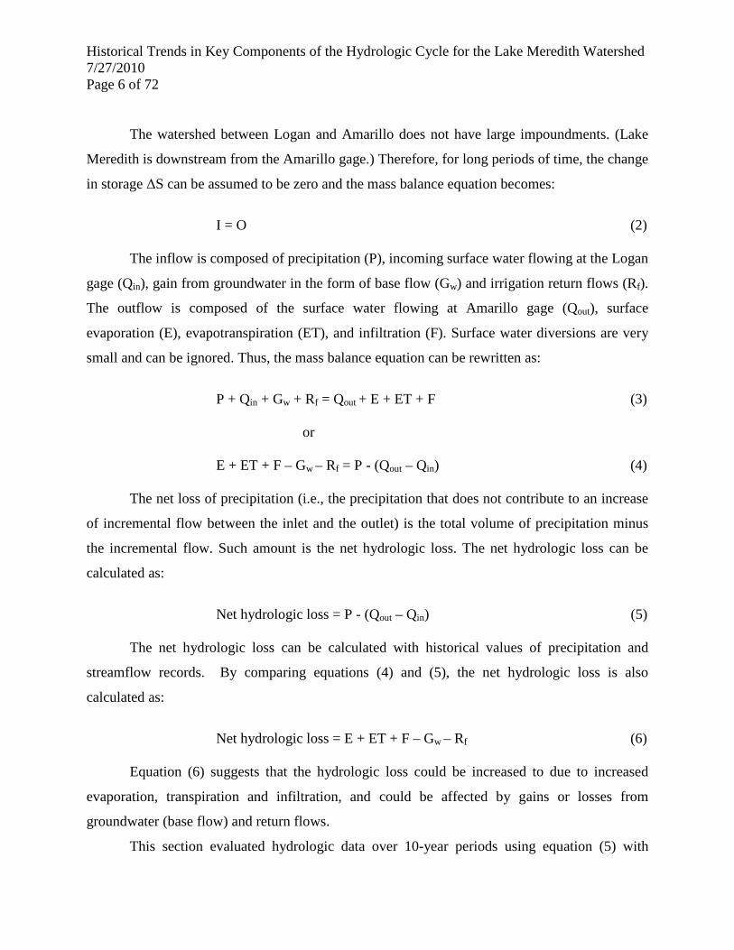
The watershed between Logan and Amarillo does not have large impoundments. (Lake

Meredith is downstream from the Amarillo gage.) Therefore, for long periods of time, the change

in storage ΔS can be assumed to be zero and the mass balance equation becomes:

I = O (2)

The inflow is composed of precipitation (P), incoming surface water flowing at the Logan

gage (Qin), gain from groundwater in the form of base flow (Gw) and irrigation return flows (Rf).

The outflow is composed of the surface water flowing at Amarillo gage (Qout), surface

evaporation (E), evapotranspiration (ET), and infiltration (F). Surface water diversions are very

small and can be ignored. Thus, the mass balance equation can be rewritten as:

P + Qin + Gw + Rf = Qout + E + ET + F (3)

or

E + ET + F – Gw – Rf = P - (Qout – Qin) (4)

The net loss of precipitation (i.e., the precipitation that does not contribute to an increase

of incremental flow between the inlet and the outlet) is the total volume of precipitation minus

the incremental flow. Such amount is the net hydrologic loss. The net hydrologic loss can be

calculated as:

Net hydrologic loss = P - (Qout – Qin) (5)

The net hydrologic loss can be calculated with historical values of precipitation and

streamflow records. By comparing equations (4) and (5), the net hydrologic loss is also

calculated as:

Net hydrologic loss = E + ET + F – Gw – Rf (6)

Equation (6) suggests that the hydrologic loss could be increased to due to increased

evaporation, transpiration and infiltration, and could be affected by gains or losses from

groundwater (base flow) and return flows.

This section evaluated hydrologic data over 10-year periods using equation (5) with


historical precipitation and streamflow records from 1950 to 2006. The hydrologic loss is

expressed as a percentage of the total precipitation. From equation (6), any historical increase in

net hydrologic loss over time could possibly be explained by one or more of the following

activities:

• Increase in evaporation due to additional surface water impoundment (examples

include SCS structures and livestock ponds)

• Increase evapotranspiration due to additional crops or the presence of more

vegetation that consumes water (for example, salt cedar)

• Reduction in groundwater inflow due to lower groundwater levels

• Reduction of return flows

• Increase of infiltration due to land leveling or other factors

• Increased surface water diversions

• Climatic variation which may include changes in precipitation, rainfall intensities,

and temperature

2.2. Methodology

To obtain values of the hydrologic loss within the watershed, available data from various

precipitation and streamflow gages were collected for the period of record 1940-20061

For each of the 6 decades studied, chosen gages were loaded in the ArcMap application.

.

Precipitation gages within the watershed area include 46 gages in Texas, 59 in New Mexico, 14

in Oklahoma, and 1 in Kansas. Not all of the gages have continuous records. Gages to be used in

the analysis for a given decade were selected based on the availability of data; in most cases,

gages with less than 60 days of missing precipitation records in a decade were selected. For

instance, between 1997 and 2006, 6 gages were used in Texas, 7 in New Mexico, 1 in Oklahoma,

and 1 in Kansas. For periods of missing data, nearby gages were analyzed to be sure a large

storm did not occur in the area, which could affect precipitation totals. If a large storm did

occur, precipitation data of nearby gages were averaged to fill in missing records.

1 Precipitation gage data were obtained from the NOAA Cooperative Extension Network (COOP). Streamflow gage data was obtained from USGS.


The average annual precipitation for the entire watershed was estimated with the Inverse

Distance Weighted (IDW) interpolation method. The IDW interpolation method calculates the

precipitation at any point of the watershed as a weighted average of the precipitation gages

around the point, where the weight of each gage is inversely proportional to the distance to the

point. In this case, as the distance from a particular precipitation gage increases, it is reasonable

to assume the precipitation estimate is less influenced by the gage and more weight is given to

closer gages. The process produces a precipitation raster with resolution of 500 meters. (That is a

grid with cells of size 500 m x 500 m where precipitation estimates are calculated for each cell).

The average annual precipitation for the watershed is calculated as the average of all its raster

cells. As an example, Figure 4 displays the average annual precipitation map for the 1950-1959

period. Maps of average annual precipitation for each decade from 1940 to 2006 are included in

Attachment A.


Figure 4. Average Annual Precipitation from 1950 to 1959

4


The mass balance method described in Section 2 was then used to calculate percent

hydrologic loss. This calculation depends on the average annual precipitation calculations for

each decade, and average annual flow into and out of the watershed based on data from the

Logan and Amarillo Canadian River stream flow gages. The total volume of precipitation

volume (P) for the decade is calculated as the annual average precipitation times the total

drainage area. The hydrologic loss as a percentage of the precipitation volume is:

% hydrologic loss =P

QQP inout )( −−

(7)

In Equation 7, precipitation is the volume over the total drainage area. Precipitation over non-

contributing area flows to a closed basin and is accounted as a loss. The hydrologic loss could be

calculated using only contributing area. This number based on contributing areas is smaller

because the loss from closed basin is removed. However, as long as the calculation area is

consistent throughout the decades, either method should reflect the same historical trend of loss.

2.3. Results

Figure 5 provides the basic trend in hydrologic loss for the Lake Meredith watershed for

the 6 decades selected for this study.


Figure 5. Hydrologic Loss per Decade

Between 1940 and 2006, hydrologic loss increased over time from 94.7% to 99.0%,

resulting in less runoff (as a percent of precipitation) reaching Lake Meredith. These results can

also be expressed as a percent rainfall/runoff. In the 1940-1949 decade, 5.3% of the precipitation

reached the Amarillo gage. In the last decade, the ratio was reduced to 1%. For reference

purposes, Lake Meredith and Ute Reservoir began impounding the Canadian River in 1965 and

1962, respectively.

Attachment A contains the maps of average annual precipitation for the six decades in

this study. Annual average precipitation and percent hydrologic loss are labeled. While there is

no trend in annual average precipitation over time, hydrologic loss has clearly increased.

Between decades 1960-1969 and 1970-1979, hydrological loss increases by 9.42%, compared to

a 0.18% increase between 1970-1979 and 1980-1989.

2.4. Conclusions

Hydrologic losses across the Lake Meredith watershed have increased over time.

Preliminary trends of precipitation data show no corresponding decrease in annual precipitation

amounts over the period of record. Losses have increase from 94.7% to 99% in 60 years. In other

94.7%

96.9%97.5%

98.3% 98.3% 98.4%99.0%

92%

93%

94%

95%

96%

97%

98%

99%

100%

1940

-194

9

1950

-195

9

1960

-196

9

1970

-197

9

1980

-198

9

1990

-199

9

1997

-200

6

Period of Record

Hyd

rolo

gic

Loss


words, the portion of the precipitation on the watershed reaching the Amarillo gage has

decreased from 5.3% to 1%. These findings imply that the watershed is losing its ability to

generate runoff. Further analyses of changes in climatic variations, groundwater levels and land

use over time may provide more information about the watersheds changing hydrology.

3.0. CLIMATIC VARIATION

Climate change is affecting temperatures and precipitation patterns worldwide. Climatic

variation could be responsible for decreased flows in the Lake Meredith watershed. Evaporation

is an important avenue of hydrologic loss. Air temperature is as an indicator of potential

evapotranspiration (Hamon, 1961). Actual evaporative losses also consider surface area of

impounded or retained water and wind. Increases in stored water in the basin are discussed under

land use, Section 5. This section focuses on the potential for climatic factors to impact

hydrologic loss. Annual and seasonal trends in maximum and minimum temperatures are

investigated in Section 3.1. Precipitation trends are presented in Section 3.2.

3.1. Temperature Trends

Temperature records from 1949 to 1999 were examined for the Lake Meredith watershed.

The objective of this analysis is to identify trends in average annual and seasonal temperature

values and determine if correlations exist between historical trends in the ratio of rainfall to

runoff and temperature. Trends in historical temperature variability were evaluated using

modeled land surface temperatures from a study by Maurer et al. (2002). The temperature dataset

was modeled at a 3-hr time step and subsequently aggregated to a monthly time step with a

spatial resolution of 1/8 degree (approximately 12 sq. km). Temperatures for each time step were

interpolated using an asymmetric spline through the daily maxima and minima. For more

information on how the dataset was developed, please refer to the study by Maurer et al.

3.1.1. Trends in Annual Maxima and Minima

This study uses the dataset developed by Maurer et al (2002) described above to extract

the 194 control points within or near (within 5 miles of) the Lake Meredith watershed. The

annual average maximum and minimum temperatures were calculated for each gridded point in


the Lake Meredith watershed. At each data point, trendlines were fit to the annual averages using

linear least-squares regression (Stafford et al, 2000). The slopes of these 194 regression lines are

mapped using the Inverse Distance Weighted (IDW) method of interpolation to assign weight to

each station. Figures 6 and 7 show the change in maxima and minima temperatures in degrees

Celsius over the 51 year period. A positive value indicates that temperatures have been

increasing, while a negative value indicates that temperatures have been decreasing.

Figure 6 shows the annual maximum temperature has decreased throughout the entire

watershed with the most rapid decreases occurring in the central-western portion. Figure 7 shows

the annual minimum temperature has decreased in some parts of the watershed and increased in

others. The increases in average annual minima are concentrated in the northwestern and

southwestern portions of the watershed, while the deceases occur in the central and eastern

portions of the watershed.

Figure 6. Change in Average Annual Maxima Temperature from 1949 to 1999 (in Celsius)

using regression lines unique to each point


Figure 7. Change in Average Annual Minima Temperature from 1949 to 1999 (in Celsius)

using regression lines unique to each point

Figure 8 is a plot of the average annual maxima and minima temperatures for the Lake

Meredith watershed with linear least squares regression lines. The trends are generally linear

over time with deviations due primarily to interannual variability. Very little change is observed

in the minima, while the temperature decrease of the maxima is more pronounced. The lack of

change in the average annual minima is likely the result of averaging, as temperature in some

parts of the watershed increased while it decreased in other areas. The regression lines indicate

that the temperature range between minima and maxima has decreased since 1949. The

coefficient of determination (R2) for these trends is relatively low. The statistical significance of

the trend still needs to be evaluated.


Figure 8. Average Annual Maxima and Minima Temperature for Lake Meredith

Watershed

3.1.2. Seasonal Trends

The procedures outlined in Section 3.1.1. were applied to analyze trends in the seasonal

minima and maxima temperatures. Seasonal temperature values are the averages of monthly

values. Seasons were defined as closely to their naturally occurring dates as possible while

preserving complete months (i.e. winter = Jan-Mar, spring = Apr-Jun, etc). This definition of

seasons has the added benefit of having all seasons occur within the same year.

Time series graphs were plotted for each of the 194 centroids for the 51 year period-of-

record. A linear least-squares regression line was then fitted to each time series. The change in

temperatures from 1949 to 1999 was calculated from the end points of the regression line. The

coefficient of determination (R2) for these trends is relatively low. The statistical significance of

the trend still needs to be evaluated.

y = -0.0196x + 21.959

y = 0.0004x + 4.867

0

2

4

6

8

10

12

14

16

18

20

22

24

26

1949

1951

1953

1955

1957

1959

1961

1963

1965

1967

1969

1971

1973

1975

1977

1979

1981

1983

1985

1987

1989

1991

1993

1995

1997

1999

Tem

pera

ture

(deg

rees

Cel

sius)

Average Annual Maxima Average Annual Minima

Values shown are averages (for the entire watershed)of annual averages for individual control points


Figure 9. Average Seasonal Maxima Temperature for Lake Meredith Watershed

Figure 10. Average Seasonal Minima Temperature for Lake Meredith Watershed

y = -0.0068x + 13.16

y = -0.0206x + 26.754

y = -0.0194x + 31.106

y = -0.0316x + 16.817

0

5

10

15

20

25

30

35

1949 1954 1959 1964 1969 1974 1979 1984 1989 1994 1999

Seas

onal

Tem

pera

ture

Max

ima

(deg

rees

C

elsi

us)

Winter Spring Summer Fall

y = 0.0187x - 4.4453

y = -0.0069x + 9.3673

y = -0.0032x + 14.982

y = -0.0069x - 0.4357

-10

-5

0

5

10

15

20

1949 1954 1959 1964 1969 1974 1979 1984 1989 1994 1999

Seas

onal

Tem

pera

ture

Min

ima

(deg

rees

C

elsiu

s)

Winter Spring Summer Fall


Maps similar to Figures 6 and 7 were generated for average seasonal maxima and minima

temperatures. These maps are included in Attachment B.

3.1.3. Range

Mean temperature ranges for each of the 51 years and 194 centroids were obtained by

subtracting monthly minima from monthly maxima and averaging them annually and seasonally.

Time series graphs were plotted for each of the centroids for the 51 year period-of-record. A

linear least-squares regression line was then fitted to each time series of temperature ranges. The

change in temperature ranges from 1949 to 1999 was calculated from the end points of the

regression line. Basin-wide averages of annual and seasonal changes in temperature range are

presented in Table 1.

Table 1. Change in Temperature Range from 1949 to 1999 Annual and Seasonal means for the Lake Meredith watershed

Annual Winter Spring Summer Fall

Range -1.0 -1.3 -0.7 -0.8 -1.2

As can be seen in Figures 6 through 8, both the maxima and the minima annual

temperatures are decreasing over significant portions of the Lake Meredith watershed but the

maximum temperature is decreasing more rapidly than the minimum. As a result, the annual

mean temperature range is decreasing with time. While all seasons show decreases in

temperature ranges, winter and fall show the most pronounced decreases.

3.1.4. Three and Five Year Moving Averages

Figure 11 shows the 3 and 5 year moving averages for annual maxima temperature.


Figure 11. Three and Five Year Moving Averages for Maxima Annual Temperature

3.1.5. Temperature Trend Conclusions

The annual maxima temperature has decreased throughout the entire watershed with the

most rapid decreases occurring in the central-western portion. The annual minima temperature

has decreased in the northwestern and southwestern portions of the watershed and increased in

the center and eastern portions of the watershed. On average, the average annual maxima have

decreased around 1 degree Celsius in the Lake Meredith watershed while the average minima

have changed very little.

18

19

20

21

22

23

24

1949 1954 1959 1964 1969 1974 1979 1984 1989 1994 1999

Max

ima

Tem

pera

ture

(deg

rees

Cel

sius)

1 yr avg 3 yr avg 5 yr avg

Annual Average

3 yr Moving Average

5 yr Moving Average

y = -0.0196x + 21.959R² = 0.1453

y = -0.023x + 22.06R² = 0.3724

y = -0.0237x + 22.1R² = 0.4897


Air temperature affects the rate of evaporation. Hamon (1961) derived an equation for

calculating potential evapotranspiration that depends only on air temperature and hours of

daylight. The Hamon Equation is expressed as

𝐸𝑇 = 0.55𝐷2 �4.95𝑒(0.062𝑇𝑎)

100� (8)

where ET is potential evapotranspiration (inch/day), D is the hours of daylight for a given day (in

units of 12 hrs) and Ta is the daily mean air temperature (°C) (Xu and Singh, 2001). Daylight is a

function of latitude and day of the year (Forsythe et al, 1995). The ratio on the right hand side is

the saturated water vapor density term which is defined as a function daily mean air temperature

(°C). As can be seen in the Hamon equation, with lower average temperatures we would expect

lower rates of evaporation.

3.2. Precipitation Trends

This section presents a statistical analysis of the historical annual precipitation in the

watershed of the Canadian River between Logan and Amarillo. The analysis was divided in three

groups:

• Basic statistics

• Trend analysis

• Persistence analysis

Historical precipitation records were obtained from the Cooperative Extension Network

operated by the National Oceanography and Atmospheric Administration (NOAA) for 191 gages

around the study area. These gages are shown in Figure 12.


Figure 12. Location of 191 Stream Gages around the Study Area

Most of the gages have short period of record or have multiple missing periods. Only a

few gages have multiple decades of continuous records. Two gages have records as early as

1904. For purposes of the development of the statistical analysis of precipitation, 21 gages with a

period of record of 50 years or more were selected. Although the records are mostly complete,

the selected 21 gages have a few missing days or months. Data for nearby gages were used to fill

in missing values for the selected 21 gages.


3.2.1. General Description of Historical Precipitation

The methodology and results for the calculation of historical precipitation are discussed

in the following sections.

3.2.1.1. Methodology

The area of study is the Canadian River watershed between Logan and Amarillo and the

period of record is 1904-2006. Daily precipitation records were obtained for 122 gages from the

National Oceanographic and Atmospheric Administration (NOAA). All of these gages are

located within or near the watershed. Records for two gages go back to 1904.

The average annual precipitation was calculated for the geographic region located

between latitude N34.75 and N37.00 and longitude W104.50 and W101.25. This region

encompasses the entire watershed of interest. A grid was drawn over this region, with lines every

1/8 of a degree. Daily precipitation for the period 1904-2006 was estimated for the corners of the

grid using the inverse distance weighted (IDW) average method. The method calculates a

weighted average of precipitation using data from nearby gages, where closer gages have more

weight than gages far away. After the daily precipitation records were calculated for each corner

of the grid, the daily average for the region was calculated as the average of all the points.

The accuracy of the precipitation for each point depends on the number of gages. The

number of gages with available records changes from 2 in 1904 to 84 in 1950. After the 1960

decade the number of gages decreases. In 2006, 40 gages were used.

3.2.1.2. Results

Historical annual precipitation in gages in the vicinity of the study area has ranged

between 5.5 inches and 44.8 inches. The average annual precipitation in the watershed between

Logan and Amarillo is 16.8 inches. This average is calculated based on estimated precipitation

across the watershed using the inverse distance weight interpolation method. The average

precipitation in the study area increases from west to east. The average precipitation in Conchas

Dam, the most western gage, is 14.5 inches while the average precipitation in Spearman, the

most eastern gage, is 20.9 inches. Two wet years occurred in 1923 and 1941. Precipitation was

remarkably high in 1923 in the southeast corner of the study area when the Claude and


Panhandle gages had a precipitation of 45 and 43 inches respectively (or more than twice the

normal rainfall). Precipitation in the western portion was not as high, but was still well above

average. In 1941, rainfall had less spatial variability as the precipitation in the area was between

31 and 40 inches. Other wet periods are 1948-1950, 1957-1961, and 1984-1988.

The most severe droughts (in terms of precipitation) occurred during the periods 1933 –

1937 and 1951 – 1956. These periods have three or more consecutive years below normal

rainfall. Other less severe droughts occurred between 1962 and 1964, 1973 and 1978, and 2000

and 2003.

Generally, hydrology in the region tends to switch between a period of drought followed

by wet years. As is discussed below, a persistence test suggests that a fluctuation between

drought and wet years occurs every 3 to 5 years.

3.2.2. Trends in Precipitation

Five gages with more 59 consecutive years of records were selected for a trend analysis.

These gages are: Canyon, TX (1924-2006), Conchas Dam, NM (1948-2006), Elkhart, KS (1912-

2006), Spearman, TX (1921-2002) and Tucumcari, NM (1905-2006). The existence (or non-

existence) of a trend was verified with the following parameters:

• Moving average every 3, 5, 10 and 50 years.

• Correlation analysis with past values

Trends in time series can be identified using a lag-one differential. The lag-one

differential obtains a new time series from the difference between two consecutive values. If the

mean of this new series is different from zero, then it is likely that the original time series has a

trend.

Y(t) = X(t+1) – X(t)

Detailed trend analyses, including the moving averages and correlation with past values, are

shown in Attachment C. Analysis of moving average and correlation with past values do not

identify any significant trend of precipitation over time for the gages at Canyon, Elkhart,


Spearman, and Tucumcari. The annual precipitation at Conchas Dam exhibits an increasing trend

of precipitation over time of 0.09 inches per year.

3.2.3. Persistence Analysis

Persistence of annual precipitation is the correlation of the precipitation at any given year

with its immediate past values. If a precipitation series has persistence, the annual precipitation

in the current year is somewhat dependent on the precipitation during one or more preceding

years. For example, if a region is experiencing a drought, the probability that the next year will

be dry is higher than the probability of having a wet year. In contrast, during a wet spell, the

probability of a wet year is higher than the probability of a dry year. It is very common for

hydrologic series to have persistence.

Hydrologic variables such as annual precipitation may have persistence, also known as

autocorrelation. Persistence reflects the degree of dependency on previous values. For example,

if a year is dry, a dry year has more probability to follow than a wet year, and a several

consecutive years may follow until a wet year occurs. When a wet year occurs, there is some

probability of a starting a series of consecutive wet years. As a result, the series may have a

tendency to fluctuate between wet and dry periods.

Persistence is usually measured by autocorrelation. Autocorrelation is a standard

correlation coefficient of the series with its own past values. A lag-time needs to be defined to

calculate the autocorrelation. For example, a lag-one autocorrelation is the correlation of today

with yesterday. A lag-two autocorrelation is the correlation of today with the values 2 days ago,

and so on. One can plot the autocorrelation values of lag-n versus n. This graph is called the

autocorrelogram. The autocorrelogram can be useful for determining cycles in time series. For

example, in monthly data that reflect yearly seasonality, the lag-12 is higher, which indicates a

cycle occurs every 12 months. In this example, this result is somewhat obvious. But if the length

of the cycle is unknown, the length of the cycle in the autocorrelogram may provide a hint. The

autocorrelogram was calculated for the annual average precipitation in the study area.

In this study, persistence was evaluated with two parameters:

• Correlation coefficients with past values (plotted in a graph called correlogram)

• Conditional frequency duration curves


The analyses were performed for the same 5 gages used in the trend analysis and are

presented in Attachment C. This analysis did not identify any large persistence in the hydrologic

series.

3.2.4. Trends in Rainfall Intensity

While rainfall totals have remained relatively constant, rainfall events in recent years may

lack the intensity and duration needed to generate significant run-off. The purpose of this section

is to verify whether such a trend can be observed in daily precipitation data from the region.

The analysis of rainfall intensities uses four of the gages used in the previous trend

analyses: Tucumcari, NM (1905-2006), Canyon, TX (1924-2006), Spearman, TX (1921-2002)

and Elkhart, KS (1912-2006). The analysis is performed by applying trend detection techniques

to the average number of rainy days (precipitation > 0 in.) per year and the average rainfall

intensity (in/day) per rain day. The techniques involve plotting a trendline using linear least-

squares regression to determine the rate of change and average deviations from the trendline. The

linear correlation coefficient (r) is used to detect correlations between rainfall intensity or

number of days and the year. Statistical significance is determined using the nonparametric

Mann-Kendall test.

The results of the analyses are shown in Tables 2 and 3. In Table 2, the rate of change

(i.e. the slope of the trendline) for the number of rainy days per year is positive for all gages. The

slope is less for the Elkhart gage. This implies an increasing trend. The average deviation from

the trendline is consistently around 10 days, with the exception of the Elkhart gage (8.7 days).

The Linear Correlation Coefficient shows positive correlations between the years and the number

of days with rain, which means that as years advance, the number of days of rain per year

increases. This increasing trend in the number of rainy days has a greater than 99% confidence

level for Tucumcari, Spearman, and Elkhart.

In Table 3, the rate of change for rainfall intensity is negative for all gages. The slope is

less for the Elkhart gage. This implies a decreasing trend in rainfall intensity. The average

deviation from the trendline is consistently around 0.06 in/day. The Linear Correlation

Coefficient shows negative correlations between the years and rainfall intensity, which means


that as years advance, rainfall intensity decreases. This decreasing trend in rainfall intensity has a

greater than 95% confidence level for Tucumcari, Canyon, and Spearman. No clear trend exists

for the Elkhart gage.

Table 2. Trends in the Average Number of Rainy Days per Year

Rate of Change

(days/yr)

Average Deviation from Trendline (+/-)

Linear Correlation

Coefficient (r)

Significance Level

Tucumcari 0.1853 9.7969 0.4104 99.998Canyon 0.1213 10.1951 0.2217 94.800

Spearman 0.1684 9.8902 0.2964 99.609Elkhart 0.0968 8.7000 0.2242 99.682

Table 3. Trends in the Average Annual Precipitation Intensity

Rate of Change

(in/day/yr)

Average Deviation from Trendline (+/-)

Linear Correlation

Coefficient (r)

Significance Level

Tucumcari -0.0011 0.0639 -0.3435 97.323Canyon -0.0011 0.0626 -0.3021 98.212

Spearman -0.0012 0.0609 -0.3563 99.680Elkhart -0.0003 0.0593 -0.1133 47.330

The return interval for high intensity rain events (>2 in/day) was also considered.

Preliminary results are based on an analysis of four gages: Amarillo WSO Airport, TX (1948-

2006), Pasamonte, NM (1948-2006), Bravo, TX (1948-2006), and San Jon, NM (1948-2006).

The analysis looked at the number of days between high intensity rain events. Amarillo,

Pasamonte and Bravo gages show increasing trends in the number of days between heavy rain

events. This pattern does not hold true for the San Jon gage. The statistical significance of these

trends still needs to be evaluated.

3.2.5. Precipitation Trend Conclusions

Precipitation data was collected from five gaging stations near the Panhandle, with a

maximum period-of-analysis from 1905-2006. During this period, the average number of rain


days has shown a more significant positive trend than total precipitation. Consequently, rainfall

intensity has a negative trend. There also appears to be an increasing interval between

significant rain events (large storms).

4.0. GROUNDWATER – SURFACE WATER INTERACTIONS

The objective of this section is to analyze trends in groundwater levels and determine if

correlations exist between historical trends in the rainfall to runoff ratio and groundwater. If

changes in groundwater levels are affecting spring flows, they could be contributing to the

decline in inflow to Lake Meredith. Trends in historical groundwater levels in the Northern

Ogallala aquifer were evaluated using modeled potentiometric head surfaces developed by

Dutton (2004). Changes in groundwater levels for the Dockum aquifer were estimated using well

data and water levels reported to the TWDB.

4.1. Change in Groundwater levels in the Ogallala

The analysis of groundwater levels in the Northern Ogallala uses the dataset developed

by Dutton (2004) to determine the extent to which groundwater levels have changed since 1950.

For more information on how the dataset was developed, please refer to the study. The change in

groundwater levels from 1950 to 1998 is presented in Figure 12. The map was generated by

subtracting the potentiometric head surfaces in 1950 from the head surfaces in 1998. Where the

value is positive, groundwater levels have risen since 1950. Where the value is negative,

groundwater level have dropped by the amounts indicated in the legend. Moore County

experienced the greatest decreases since 1950 (decreases of up to 200 ft). Sherman, Dallam,

Carson, Hartley, Hutchinson, and Hansford Counties experienced draw-downs of up to 120 ft.

The other counties of the PWPA experienced less significant drawdowns.

There are three named springs within the Lake Meredith watershed that overlie the

Northern Ogallala aquifer: Bravo Springs, XIT Springs, and Alibates Springs. The flow in these

and surrounding springs could be affected by decreases in groundwater levels in the Northern

Ogallala.

The Bravo Springs are located in the northwest corner of Oldham County where draw-

downs over the past 50 years have not exceeded 20 ft. For this reason, significant reductions in


spring flow at this site due to decreased groundwater levels are unlikely. The flow in Bravo

Springs was 1.1 liters per second (lps) on June 22, 1971 and 1.4 lps on May 4, 1977 (Brune,

1981). The XIT Springs are located in Hartley County, approximately 9 miles to the southwest of

Hartley, Texas. While water levels have changed only slightly since 1950 underneath the spring

itself, draw-downs of up to 120 feet have occurred around Hartley. The flow in this spring could

be affected by pumping groundwater. Flow in the XIT Springs was probably larger and

continuous in the 19th century. By 1981, however, flow in the springs ceased for three or four

months out of the year due to irrigation pumping (Brune, 1981). Alibates Springs are located in

the northwest corner of Potter County and may be affected by areas of increased draw-down

within 10 miles to the southwest.

4.2. Changes in Groundwater Levels in the Dockum

Changes in historical water levels in the Dockum Aquifer could be contributing to

declining lake levels in Lake Meredith. The Dockum aquifer lies beneath much of the Meredith

watershed and is the only aquifer present beneath the Canadian River. The break in the Ogallala

corresponds with a Dockum outcrop.

The following information was used to build a dataset of water levels in wells drawing

from the Dockum Aquifer:

1) Text file containing well information from TWDB website

2) Text file containing historical water levels from TWDB website


Figure 12. Change in Groundwater Levels in the Ogallala Aquifer from 1950 to 1998.


The text file containing well information includes data on latitude, longitude, and land

surface elevations at each well. Historical water levels are reported as depth from land surface.

Water levels were determined by subtracting the depth to water surface from the land surface

elevation. Next, decadal averages were calculated for the water level in each well. The average

water levels were appended to the well records and the wells were added to ArcMap using the

XY coordinates.

The wells chosen for this study comply with the following criteria:

Identified by the TWDB as being drilled in one of the formations listed in Table 4.

… or ….

Located within the Ogallala break

… and …

Located within the Lake Meredith watershed or within 35 miles of its boundary.

Table 4. Dockum and Dockum Related Formations

CODE FORMATION 100CPDG CENOZOIC PECOS ALLUVIUM AND DOCKUM FORMATION

100CPDR CENOZOIC PECOS ALLUVIUM, AND DOCKUM AND RUSTLER FORMATIONS

110AVDK ALLUVIUM AND DOCKUM FORMATION 121OGDK OGALLALA FORMATION AND DOCKUM FORMATION 218ASDG ANTLERS SAND AND DOCKUM FORMATION

218EDAD EDWARDS AND ASSOCIATED LIMESTONES, ANTLERS SAND, AND DOCKUM FORMATION

231DCKM DOCKUM FORMATION 231DCKP DOCKUM FORMATION AND PERMIAN ROCKS


Seven hundred twenty-one (721) wells with a total of 4,633 records meeting the criteria above

were identified. These records span a period of time from pre-1950s to 2009. Table 5 shows the

distribution of wells and well records by decade.

Table 5. Number of Wells and Well Records meeting the Criteria Above

Potentiometric head surfaces were developed on a decade by decade basis using the

Ordinary Kriging interpolation method with a spherical semivariogram model. Kriging is an

advanced geostatistical technique that is used in hydrogeology to interpolate groundwater levels

at any point of the area of analysis based on the available well data (Sun et al, 2009). For

example, the head surface map for the 1960s was estimated using the kriging interpolation

method based on the 483 well records between 1960 and 1969. For more information, please

consult the extensive body of work on kriging as a method of interpolation in GIS (Heine, 1986;

Oliver, 1990; McBratney and Webster, 1986).

In order to determine the change in head surfaces between decades, the head surface from

the earlier decade is simply subtracted from the head surface of the later decade. Data from the

1950s was not used in this analysis because greater modeling uncertainties are introduced by the

limited well data. The estimated change in head surfaces from 1960 to 2009 in the Dockum

aquifer is shown in Figure 13. It can be seen in Figure 13 that the area of greatest drawdown

occurs below Lake Meredith and the 30 miles of the Canadian River leading up to the reservoir.

According to this analysis, groundwater levels have dropped by more than 250 ft in some areas

of the watershed since the 1960s.

DecadeNumber of

Wells

Number of Well

Records1950-1959 37 551960-1969 231 4831970-1979 299 8061980-1989 327 10791990-1999 145 8622000-2009 186 1345


Figure 13. Estimated change in potentiometric head surfaces from the 1960s to the 2000s.

Differences in Dockum groundwater levels between successive decades were also

considered. The metrics used to assess the change in groundwater levels are the Mean Absolute

Relative Error/Difference (MARE), the Mean Relative Error (MRE), and the percent of the

Canadian River (considering the 125 miles between the Texas border and Sanford Dam) that the

previous decade water levels were higher than the later decade.


The mean absolute relative error (MARE) is calculated using Eq. 9 (Dawson et al., 2007).

∑=

−=

n

ioi

si

oi

Q

QQ

nMARE

1

100 (9)

Where n is the number of data points, Qi is the groundwater level at point i along the Canadian

River, Qo is the groundwater level in the earlier decade, and Qs is the groundwater level in the

later decade. MARE is a non-negative metric with no upper bound. In this study, the MARE is

used to describe the change in groundwater levels between decades. A value of zero for MARE

would mean there is no change in groundwater levels between decades. Because the metric uses

the absolute difference between simulated and observed values, it is not as sensitive to large

errors as the difference squared. The mean absolute error (MAE) may also be used for this type

of assessment.

The MRE is formulated in a way similar to Eq. 9 except that the signed value of the

difference between decades is taken instead of the absolute value. When MRE is positive, the

earlier decade is greater than the later decade. When MRE is negative, the opposite is true. It is

used in conjunction with the MARE because negative and positive errors will cancel each other

out, so it is possible to approach zero even when successive decades are not similar.

Table 6 shows that the two successive decades with the greatest differences in

groundwater levels are the 1960s and the 1970s. Differences between the 1990s and 2000s are

also large in comparison to other decades. This suggests that the rate of drawdown has increased

in recent years. A plot of historical storage contents in Lake Meredith is shown in Figure 2.

Historical streamflow at the Amarillo gage is shown in Figure 3. It is possible to see in Figures 2

and 3 that while streamflows and storage levels may have been declining for the past few

decades, it was not until around 2000 that a precipitous decline is observed. This could be related

to the increasing draw down in Dockum water levels during the same period of time.


Table 6. Differences in Dockum Groundwater Levels between Successive Decades

4.3. Base Flow Analysis

A preliminary analysis of base flows was also conducted. Base flows enter stream

channels from groundwater. It is the portion of stream flow attributable to groundwater and not

runoff. Base flow separation techniques use gaged stream flows to derive a base flow signature.

Two commonly-used techniques are the recursive method and the local minima method.

The Local Minima Method compares the slope of the hydrograph and connects the points

located at local minima (Lim et al., 2005). The recursive method separates base flow based on

the assumption that the outflow from an aquifer is proportional to its storage (Eckhardt, 2005).

The results of applying these methods to stream flows at the Amarillo gage are presented

in Figures 14 and 15. Implementation of these methods was facilitated using the Web-based

Hydrograph Analysis Tool (WHAT) developed at Purdue University.

At least two observations can be made from Figures 14 and 15: 1) base flows contribute a

considerable amount of water to stream flows in the Canadian River, and 2) base flows exhibit a

decreasing trend (as total stream flows also do as shown on Figure 3).

Time Period MARE MRE

% of river with earlier decade

higher than later decade

1960s - 1970s 3.217 2.601 851970s - 1980s 2.202 -1.629 381980s - 1990s 1.782 -0.916 411990s - 2000s 2.074 1.684 64


Figure 14. Base Flows as determined using the Recursive Method

Figure 15. Base Flows as determined using the Local Minima Method

The tremendous variability in base flows seen in Figures 14 and 15 is likely an artifact of

the separation techniques, which are based entirely on gaged flows. Other base flow separation

methods should be investigated. Adjustments can be made to account for releases from Ute

Reservoir, which may be mistakenly identified as base flow.

4.4. Groundwater Conclusions

y = 40163e-0.014x

R² = 0.1183

1

10

100

1000

1939

1943

1947

1951

1955

1959

1963

1967

1971

1975

1979

1983

1987

1991

1995

1999

2003

2007

Base

Flo

w (t

hous

ands

of a

c-ft

)

Recursive method

y = 37938e-0.013x

R² = 0.081

1

10

100

1000

1939

1943

1947

1951

1955

1959

1963

1967

1971

1975

1979

1983

1987

1991

1995

1999

2003

2007

Base

Flo

w (t

hous

ands

of a

c-ft

)

Local minima method


There have been declining groundwater levels in the aquifers within the Lake Meredith

watershed. Base flows are shown to be declining from approximately 40,000 acre-feet per year to

less than 20,000 acre-feet per year. Spring flows likely have been affected by changes in

groundwater levels, but in areas with known springs the groundwater draw downs have not been

significant. Also, the areas with the largest draw downs in the Ogallala aquifer tend to coincide

with the non-contributing portions of the watershed. Changes in historical water levels in the

Dockum aquifer appear to be the greatest along the Canadian River near Lake Meredith.

Groundwater levels have dropped by more than 250 ft in some areas of the watershed since the

1960s. The decline in inflows to Lake Meredith could be related to draw downs in Dockum

water levels during same period of time. However, the reductions in groundwater base flow

contributions are only a fraction of the observed decline in stream flows.

5.0. LAND USE

Changes in land use and land cover can have important implications for watershed

hydrology. Additional crops or the expansion of brush lands can increase hydrologic losses due

to transpiration and interception. Land cover can also affect the rate of infiltration. Increased

surface water impoundments, changes in diversions and return flows, and consideration of non-

contributing areas are also relevant.

5.1. Changes in Land Use through Time

Land use records from 1967 to 2001 were examined for the Lake Meredith watershed.

The objective of this study is to analyze changes in land use to determine if correlations exist

between historical trends in the rainfall to runoff ratio and land cover. Changes in historical land

use were evaluated using land cover datasets developed for the following years: 1967

(Marschner and Anderson, 1967), 1970 to 1985 (Price et al., 2006), 1992 (Vogelmann et al.,

2001), and 2001 (Homer et al., 2007). For more information on how each dataset was developed,

please refer to the individual studies.

An important caveat of this analysis is that the datasets were developed at different scales

and use distinct classification schemes which discourage comparisons. That said, generalized

trends can be extracted from the data if each dataset is reclassified into more general land use


categories (e.g. combining Commercial, Industrial and Residential uses into one Urban land use

category). The 1967 dataset was developed at the smallest scale (i.e. 1:7,500,000) and uses the

most general land use categories. Consequently, the 1967 dataset largely governs the scale and

classification scheme of the analysis.

Land use maps for the four years are presented in Attachment D. Since 1967, four land

use classes have occupied 99% of the land in the Lake Meredith watershed: Urban, Agriculture,

Grassland, and Shrubland. On average, these land use classes occupy 1%, 13%, 69%, and 16%

of the watershed, respectively. Graphs of how the percentage of total watershed area occupied by

each class has changed through time are presented in Figures 16 through 19.

Several trends are apparent from Figures 16 through 19. The percent of total watershed

area occupied by urban areas has increased roughly 1%. The area occupied by agricultural land

has decreased by around 9%. Grasslands have decreased by around 17% and shrublands have

increased roughly 24%. In Figure 16, the drop in Urban land class in 1992 (or conversely, the

increase in 2001) is because the mapping technique used for the 2001 dataset resulted in the

identification of more roads than could be identified in 1992 dataset.

Figure 16. Percentage of watershed area designated as Urban

Figure 17. Percentage of watershed area designated as Agricultural

0.0

0.5

1.0

1.5

1967 1985 1992 2001

% o

f Tot

al W

ater

shed

Urban

0

5

10

15

20

1967 1985 1992 2001

% o

f Tot

al W

ater

shed

Agriculture


Figure 18. Percentage of watershed area designated as Grassland

Figure 19. Percentage of watershed area designated as Shrubland

Figures 17 and 18 show that the percent of watershed area occupied by agricultural lands

and grasslands has decreased since 1967. Figures 16 and 19 show that the area occupied by

urban areas and shrublands has increased since 1967.

According to the reclassification used in this analysis, agricultural land was being lost to

grasslands at a rate of 20 square miles per year up to 1992. Around 85% of the grasslands being

lost are converted to shrublands. Much of this shrubland is associated with invasive species such

as salt cedar. Roughly 90% of the new shrubland is replacing grasslands and mixed forest.

Expanding urban areas are replacing grasslands and agricultural lands.

In short, agricultural lands have decreased by 9% and are generally being replaced by

grasslands. Grasslands have decreased by 17% and are generally being replaced by shrublands.

Shrublands have increased by around 24% and are generally replacing grasslands. Urban areas

have increased by about 1% and are generally replacing both agricultural lands and grasslands.

These trends appear to be consistent with natural succession.

The increase in shrublands (salt cedar) is occurring primarily in the southwestern portion

of the watershed and along the Canadian River. This part of the watershed typically experiences

less rainfall (between 14 and 17 inches per year) compared to other areas (see Section 3.2.).

Brush management strategies are typically more effective in areas with greater rainfall (Hibbert,

0

20

40

60

80

100

1967 1985 1992 2001

% o

f Tot

al W

ater

shed

Grassland

0

10

20

30

40

1967 1985 1992 2001% o

f Tot

al W

ater

shed

Shrubland


1983). Significant expansion of shrubland has also occurred along the Canadian River and the

watershed area draining directly to Lake Meredith as shown on Figure 20.

a.

Figure 20. Comparison of the Extent of Shrubland between 1992 (a) and 2001 (b).

The analysis presented in Figure 18 for shrubland was rerun considering only

contributing areas of the watershed. Figure 21 show that the results have changed. Since 1967,

shrubland in the contributing areas of the watershed has increased from less than 5% to nearly

35%. If the same exercise were repeated for agricultural areas, the percentages displayed in

Figure 17 would be considerably less.

b.


Figure 21. Percentage of Contributing Watershed Area designated as Shrubland

5.2. Surface Water Impoundments

This study also considered an increase in surface water impoundments as a possible

explanation for declining lake levels. The national inventory of dams was used to generate

Figures 22 and 23. Figure 22 shows the location of small dams within the watershed. Figure 23

shows the cumulative capacity of each dam and the year it was built. For example, if the first

dam was built in 1940 and had a capacity of 100 ac-ft, the cumulative capacity in 1940 would be

100 ac-ft. If the second dam was built in 1941 and had a capacity of 150 ac-ft, the cumulative

capacity in 1941 would be 250 ac-ft.

The total amount of water impounded by small dams since 1940 is around 10,000 ac-ft,

which by itself is not sufficient to explain the losses in stream flow. Impoundment of surface

water by small dams is likely playing a limited (but not negligible) role in declining stream

flows.

This analysis considers impoundment by small dams listed in the national inventory.

There were no historical and geographical data on development of small impoundments that are

not listed in the national inventory (livestock ponds, some SCS structures and others). One

indicator of the potential for development of livestock ponds is the historical livestock water

demands available through the TWDB. These demands are developed based on the number of

0

5

10

15

20

25

30

35

40

1967 1985 1992 2001

% o

f Con

trib

utin

g W

ater

shed

Shrubland


livestock and the need for water. Some of the water is met through groundwater sources and

some through the development of small impoundments. The data show that there has been an

increase in livestock demands in Hartley County from approximately 2,200 acre-feet per year

demand in 1974 to a maximum demand of over 6,000 acre-feet per year in 1997. The other

counties within the Lake Meredith watershed show only slight increases in demand. While small

impoundments are likely increasing in the watershed, these changes probably are not causing the

significant decreases in runoff observed today.

Figure 22. Location of Small Dams in Lake Meredith Watershed


Figure 23. Cumulative Capacity of Small Dams in Lake Meredith Watershed

5.3. Changes in Diversions and Return Flows

Changes in water use, including diversions and return flows, were considered in this

study. A review of the Canadian River WAM Run 8 (current conditions) reveals that water rights

for diversions made at locations besides Lake Meredith total less than 2,000 ac-ft per year.

Return flows made at locations other than Lake Meredith are less than 300 ac-ft per year.

Because the magnitude of these water use patterns is so small, it was determined that no further

investigation was required because any historical changes to the pattern would be unlikely to

affect Lake Meredith.

5.4. Land-Use Conclusions

The major land use change in the Lake Meredith watershed appears to be an increase in

shrubland (salt cedar), especially within the contributing areas of the watershed. Changes in

agricultural lands and irrigation practices likely have minimal impacts to surface water runoff

because most of these lands are located in the non-contributing areas of the watershed. Total

impoundments have increased over time and will impact runoff. However, the storage volumes

in these impoundments stabilized in the 1970s and are likely not a major contributing factor to

the precipitous declines in runoff observed in the last decade.

12000

14000

16000

18000

20000

22000

24000

26000

28000

30000

1930 1940 1950 1960 1970 1980 1990

Cum

ulat

ive

Capa

city

of S

mal

l Dam

s (a

f)

CumCapDams Year meredith was built


6.0. SUMMARY AND CONCLUSIONS

The study confirmed that the Lake Meredith watershed is losing its ability to generate

runoff and stream flow to the Canadian River. The greatest increase in hydrologic loss occurred

in the 1950s with another major increase in the last decade (1997–2006). There appears to be no

one factor or event causing the decline of inflows to Lake Meredith. Analyses of climatic factors

show little to no change in annual precipitation and decreasing temperatures. Rainfall intensities

are declining over time and significant rainfall events (>2 in/day) appear to be occurring less

frequently. Groundwater levels are declining in both the Ogallala and Dockum aquifers. Base

flows in the Canadian River also show declining trends. The decline in base flow is less than one

tenth of the decrease in stream flow at the Amarillo gage since 1939. The largest declines in the

Ogallala aquifer coincide with the non-contributing portions of the watershed, while the declines

in the Dockum are beneath Lake Meredith and 30 miles upstream along the Canadian River.

Changes in land use include reductions in agricultural and pasture lands, increases in

shrubland and increases in small impoundments. Of these changes, the increase in shrubland and

decline in pasture land has the greatest potential to impact surface water runoff. The changes in

agricultural lands (along with any changes to irrigation practices) are assumed to have minimal

impacts to runoff because most of the agricultural lands are located in the non-contributing

portions of the watershed. The increases in shrubland will increase evapotranspiration and

intercept potential runoff due to increased vegetation.

In summary, annual precipitation, potential evaporation, and changes in irrigation

practices do not appear to be contributing factors to the apparent hydrologic loss in the Lake

Meredith watershed. Changing trends in the potential contributing factors occur over decades

with no significant increase in this last decade. It is likely that the combination of factors,

including reduced rainfall intensities, increasing shrubland and declining groundwater levels,

have resulted in tipping the hydrologic balance of the watershed to the point that inflows to Lake

Meredith (generated below Ute Reservoir) is now about 20 percent of inflows observed in the

1940s. While the activities in the watershed above the Logan gage cannot be ignored with

respect to the total amount of inflow to Lake Meredith, this study confirms that changes in the

watershed below Ute Reservoir have contributed to reduced stream flows.


REFERENCES Brune, G. Springs of Texas, Volume I. Published and distributed in 1981 by Gunnar Brune, 2014 Royal Club Court, Arlington, TX. ISBN: 0-9604766-0-1. Dawson, C. W., R. J. Abrahart, L. M. See. 2007. “HydroTest: A web-based toolbox of evaluation metrics for the standardized assessment of hydrological forecasts.” Environmental Modelling & Software. 22, 1034-1052. Dutton, A. 2004. “Adjustments of parameters to improve calibration of the Og-n model of the Ogallala aquifer.” Panhandle Water Planning Area: The University of Texas at Austin, Bureau of Economic Geology, report prepared for Freese and Nichols, Inc., and Panhandle Water Planning Group, Austin, TX. Eckhardt, K. 2005. “How to Construct Recursive Digital Filters for Baseflow Separation.” Hydrological Processes. 19(2), 507-515. Forsythe, W. C., E. J. Rykiel, R. S. Stahl, H. Wu, R. M. Schoolfield. 1995. “A model comparison for day length as a function of latitude and day of year.” Ecological Modelling. 80, 87-95. Hamon, R. W. 1961. “Estimating potential evapotranspiration.” J. Hydraulics Div., American Society of Civil Engineers, 87, 107-120. Heine, G.W. 1986. “A Controlled Study of Some Two-Dimensional Interpolation Methods.” COGS Computer Contributions. 3(2), 60-72. Hibbert, A. R. 1983. “Water yield improvement potential by vegetation management on western rangelands.” Water Resources Bulletin. 19(3), 375-381. Homer, C., J. Dewitz, J. Fry, M. Coan, N. Hossain, C. Larson, N. Herold, A. McKerrow, J.N. VanDriel and J. Wickham. 2007. “Completion of the 2001 National Land Cover Database for the Coterminous United States.” Photogrammetic Engineering and Remote Sensing. 73(4), 337-341. http://www.mrlc.gov/nlcd.php Lim, K. J., B. A. Engel, Z. Tang, J. Choi, K. Kim, S. Muthukrishnan, and D. Tripathy. 2005. “Automated web GIS-based hydrograph analysis tool, WHAT.” Journal of the American Water Resources Association. pg.1407-1416, December. Marschner, F. J., and J. R. Anderson. 1970. “Major Land Uses in the United States.” The National Altas of the United States of America. U.S. Geological Survey. Washington, DC. http://water.usgs.gov/GIS/metadata/usgswrd/XML/na70_landuse.xml

http://www.mrlc.gov/nlcd.php�




http://water.usgs.gov/GIS/metadata/usgswrd/XML/na70_landuse.xml�




Maurer, E. P., A. W. Wood, J. C. Adam, D. P. Lettenmaier, and B. Nijssen. 2002. “A long-term hydrologically based dataset of land surface fluxes and states for the coterminous United States.” Journal of Climate. 15, 3237-3251. McBratney, A.B., and R. Webster. 1986. “Choosing Functions for Semi-variograms of Soil Properties and Fitting Them to Sampling Estimates.” Journal of Soil Science 37, 617-639. Oliver, M.A. 1990. “Kriging: A Method of Interpolation for Geographical Information Systems.” International Journal of Geographic Information Systems. 4, 313-332. Price, C.V., N. Nakagaki, K.J. Hitt, and R.C. Clawges. 2006. “Enhanced Historical Land-Use and Land-Cover Data Sets of the U.S. Geological Survey.” U.S. Geological Survey Digital Data Series 240. http://water.usgs.gov/GIS/metadata/usgswrd/XML/ds240_landuse_poly.xml Stafford, J. M., G. Wendler, and J. Curtis. 2000. “Temperature and precipitation of Alaska: 50 year trend analysis.” Theoretical and Applied Climatology. 67, 33-44. Sun, Y, S. Kang, F. Li, and L. Zhang. 2009. “Comparison of interpolation methods for depth to groundwater and its temporal and spatial variations in the Minquin oasis of northwest China.” Environmental Modelling & Software. 24 (10), 1163-1170. Vogelmann, J.E., S.M. Howard, L. Yang, C.R. Larson, B.K. Wylie, N. Van Driel, 2001. “Completion of the 1990s National Land Cover Data Set for the Conterminous United States from Landsat Thematic Mapper Data and Ancillary Data Sources.” Photogrammetric Engineering and Remote Sensing. 67, 650-652. Web-based Hydrograph Analysis Tool (WHAT) Website, Purdue University. http://cobweb.ecn.purdue.edu/~what/ Xu, C. Y., and Singh, V. P. 2001. “Evaluation and generalization of temperature-based methods for calculating evaporation.” Hydrological Processes. 15, 305-319.

http://water.usgs.gov/GIS/metadata/usgswrd/XML/ds240_landuse_poly.xml�



http://cobweb.ecn.purdue.edu/~what/�

http://cobweb.ecn.purdue.edu/~what/�


ATTACHMENT A

AVERAGE ANNUAL PRECIPITATION MAPS


ATTACHMENT B

SEASONAL TEMPERATURE MAPS


Figure B-1. Change in Average Winter Maxima (a) and Minima (b) Temperature from 1949 to 1999 (in Celsius) using regression lines unique to each point.


Figure B-2. Change in Average Spring Maxima (a) and Minima (b) Temperature from

1949 to 1999 (in Celsius) using regression lines unique to each point.


Figure B-3. Change in Average Summer Maxima (a) and Minima (b) Temperature from

1949 to 1999 (in Celsius) using regression lines unique to each point.


Figure B-4. Change in Average Fall Maxima (a) and Minima (b) Temperature from 1949 to

1999 (in Celsius) using regression lines unique to each point.


ATTACHMENT C

PRECIPITATION TREND ANALYSIS


Figure C-1. 3 Year Moving Average


0

5

10

15

20

25

30

35

40

1904

1909

1914

1919

1924

1929

1934

1939

1944

1949

1954

1959

1964

1969

1974

1979

1984

1989

1994

1999

2004

Aver

age

Prec

ipita

tion

(inch

es)

Annual Average3-Year MAAnnual Average

0

5

10

15

20

25

30

35

40

1904

1909

1914

1919

1924

1929

1934

1939

1944

1949

1954

1959

1964

1969

1974

1979

1984

1989

1994

1999

2004

Aver

age P

reci

pita

tion

(inch

es)





0

5

10

15

20

25

30

35

40

1904

1909

1914

1919

1924

1929

1934

1939

1944

1949

1954

1959

1964

1969

1974

1979

1984

1989

1994

1999

2004

Aver

age

Prec

ipita

tion

(inch

es)


0

5

10

15

20

25

30

35

40

1904

1909

1914

1919

1924

1929

1934

1939

1944

1949

1954

1959

1964

1969

1974

1979

1984

1989

1994

1999

2004

Aver

age

Prec

ipita

tion

(inch

es)



Figure C-5. Correlation of Average Precipitation with Past Values for the Watershed

-0.25

-0.20

-0.15

-0.10

-0.05

0.00

0.05

0.10

0.15

0.20

0.25

1 2 3 4 5 6 7 8 9 10

Cor

rela

tion

Coe

ffici

ent

Lag (Years)


Figure C-6. Conditional Probability of Exceedance for Canyon, TX

Figure C-7. Correlation with Past Values for Canyon, TX

0.0

5.0

10.0

15.0

20.0

25.0

30.0

35.0

40.0

45.0

50.0

0.00 0.20 0.40 0.60 0.80 1.00

Ann

ual P

reci

pita

tion

(Inch

es)

Probability Annual Precipitation will be Equaled or Exceeded

Conditional Probability of Exceedence

Theoretical After Below MedianYears following Below Median RainfallTheoretical After Above MedianYears following Above Median Precipitation

CANYON, TX

-0.30

-0.20

-0.10

0.00

0.10

0.20

0.30

1 2 3 4 5 6 7 8 9 10 11 12 13 14 15 16 17 18 19 20 21 22

Cor

rela

tion

Coe

ffici

ent

Lag (Years)

Correlation with Past Values

Significantly different from zero

CANYON, TX


Figure C-8. Conditional Probability of Exceedance for Conchas, NM

Figure C-9. Correlation with Past Values for Conchas, NM

0.0

5.0

10.0

15.0

20.0

25.0

30.0

35.0

40.0

0.00 0.20 0.40 0.60 0.80 1.00

Annu

al P

reci

pita

tion

(Inch

es)




CONCHAS DAM, NM

-0.30

-0.20

-0.10

0.00

0.10

0.20

0.30

0.40

1 2 3 4 5 6 7 8 9 10 11 12 13 14 15 16 17 18 19 20 21 22

Cor

rela

tion

Coe

ffici

ent

Lag (Years)



CONCHAS DAM, NM


Figure C-10. Conditional Probability of Exceedance for Elkhart, KS

Figure C-11. Correlation with Past Values for Elkhart, KS

0.0

5.0

10.0

15.0

20.0

25.0

30.0

35.0

40.0

45.0

0.00 0.20 0.40 0.60 0.80 1.00

Ann

ual P

reci

pita

tion

(Inch

es)




ELKHART, KS

-0.40

-0.30

-0.20

-0.10

0.00

0.10

0.20

0.30

1 2 3 4 5 6 7 8 9 10 11 12 13 14 15 16 17 18 19 20 21 22

Cor

rela

tion

Coe

ffici

ent

Lag (Years)



ELKHART, KS


Figure C-12. Conditional Probability of Exceedance for Spearman, TX

Figure C-13. Correlation with Past Values for Spearman, TX

0.0

5.0

10.0

15.0

20.0

25.0

30.0

35.0

40.0

45.0

50.0

0.00 0.20 0.40 0.60 0.80 1.00

Annu

al P

reci

pita

tion

(Inch

es)




SPEARMAN, TX

-0.30

-0.20

-0.10

0.00

0.10

0.20

0.30

1 2 3 4 5 6 7 8 9 10 11 12 13 14 15 16 17 18 19 20 21 22

Cor

rela

tion

Coe

ffici

ent

Lag (Years)



SPEARMAN, TX


Figure C-14. Conditional Probability of Exceedance for Tucumcari, NM

Figure C-15. Correlation with Past Values for Tucumcari, NM

0.0

5.0

10.0

15.0

20.0

25.0

30.0

35.0

40.0

45.0

0.00 0.20 0.40 0.60 0.80 1.00

Ann

ual P

reci

pita

tion

(Inch

es)




TUCUMCARI, NM

-0.25

-0.20

-0.15

-0.10

-0.05

0.00

0.05

0.10

0.15

0.20

0.25

0.30

1 2 3 4 5 6 7 8 9 10 11 12 13 14 15 16 17 18 19 20 21 22

Cor

rela

tion

Coe

ffici

ent

Lag (Years)



TUCUMCARI, NM


ATTACHMENT D

RECLASSIFIED LAND USE MAPS


ReclassificationValue Description LUC Description LUCODE Description No. Description No. Description

1 Urban 16 Urban areas 10s (11-17) Urban or built-up land 20s (21-23) Developed 20s (21-24) Developed2 Agriculture 1 Mostly cropland 21 Cropland and Pasture 81 Pasture/Hay 81 Pasture/Hay

2 Cropland with grazing land 22 Orchards 82 Row Crops 82 Cultivated Crops

3Cropland with pasture, woodland, and forest

23Confined Animal Feeding Operations

83 Small Grains

4 Irrigated land 24 Other Agricultural Land 84 Fallow

3 Grasslands 8Subhumid grassland and semiarid grazing land

31 Herbaceous rangeland 71 grasslands/herbaceous 71 grasslands/herbaceous

4 Shrubland 9Open woodland grazed (pinon, juniper, haparral and brush)

32Shrub and brush rangeland

51 Shrubland 51 Dwarf Scrub

10 Desert shrubland grazed 52 Shrub/Scrub

11Desert shrubland mostly ungrazed

5 Forest 5Woodland and forest with some cropland and pasture

41 deciduous forest land 41 Deciduous forest 41 Deciduous forest

6Forest and woodland mostly grazed

42 Evergreen forest land 42 Evergreen Forest 42 Evergreen Forest

7Forest and woodland mostly ungrazed

43 Mixed Forest 43 Mixed Forest 43 Mixed Forest

6 Wetlands 13 Swamp 61 Forested wetland 91 Woody wetlands 90-94woody, forested, and scrub/shrub wetlands

14 Marsh 62 Nonforested wetland 92emergent herbaceous wetlands

95-99emergent wetlands and aquatic bed

7 Open water 17 Open water 50s (51-54) Water 11 Open water 11 open water8 Barren land 12 Barren land 70s (71-77) Barren land 30s (31-33) Barren land 30s (31-32) Barren Land

1967 1970-1985 20011992


Figure D-1. Reclassified Land Use Map for 1967


Figure D-2. Reclassified Land Use Map for 1970-1985

20g%20-%20lake%20meredith%20study

Documents

lake meredith study

introduction lake meredith

lake meredith water

lake meredith watershed

lake greenbelt

lake merideth watershed

declining lake levels

hydrologic cycle