hp journal 1969 - correlation

HEWLETT-PACKARD JOURNAL

NOVEMBER 1969 © Copr. 1949-1998 Hewlett-Packard Co.

Correlation, Signal Averaging, and Probability Analysis

Cor re la t i on i s a measu re o f t he s im i l a r i t y be tween two wave fo rms . I t i s use fu l i n nea r l y every k ind o f research and eng ineer ing â€” e lec t r i ca l , mechan ica l , acous t i ca l ,

med i ca l , nuc lea r , and o the rs . Two o the r s ta t i s t i ca l me thods o f wave fo rm ana l ys i s -s igna l averag ing and probab i l i t y ana lys is â€” are a lso w ide ly usefu l .

By Richard L. Rex and Gordon T. Roberts

S O M E T H I N G S , L I K E T W O P E A S I N A P O D , A R E S I M I L A R ;

others, like chalk and cheese, are not. Throughout sci ence, however, we find instances where the situation is not as clear as this, and where it is desirable to establish a measure of the similarity between two quantities. Cor relation is such a measure.

As it applies to waveforms, correlation is a method of time-domain analysis that is particularly useful for de tecting periodic signals buried in noise, for establishing coherence between random signals, and for establishing the sources of signals and their transmission times. Its applications range from engineering to radar and radio astronomy to medical, nuclear, and acoustical research, and include such practical things as detecting leaks in pipelines and measuring the speed of a hot sheet of steel in a rolling mill.

Mathematically, correlation is well covered in the existing literature,1 and the use of correlation for research purposes has been established for more than a decade. Until recently, however, correlation in practice has been a complex and time-consuming operation involving, in most cases, two separate processes â€” data recording and computer analysis. For this reason, correlation tech niques could hardly be considered for routine use. Today, correlation in real time is entirely practicable, and there seems little doubt that the techniques will soon take their place in all fields of engineering and scientific research.

In this article we present the basic principles of corre lation theory. Also included are brief discussions of the concepts of signal averaging and probability density func tions. The article on page 9 describes a new HP instru ment which applies these ideas in real time, and the article on page 17 deals with applications of this instrument.

AA/V\/\A A,. v â€¢

A./!* A,. A * T

F ig . 1 . Co r re la t i on i s a measure o f t h e s i m i l a r i t y b e t w e e n t w o w a v e f o r m s . I t i s c o m p u t e d b y m u l t i p l y i n g t h e w a v e f o r m s o r d i - na te by o rd ina te and f i nd ing the a v e r a g e p r o d u c t . H e r e w a v e fo rms a ( t ) and b ( t ) a re iden t i ca l , so the co r re la t i on be tween them is la rge . Waveforms c ( t ) and d( t ) a re iden t i ca l i n shape , bu t the re i s a t ime sh i f t be tween them, so t he co r re l a t i on be tween t hem i s s m a l l e r t h a n t h a t b e t w e e n a ( t ) and b ( t ) . Hence co r re l a t i on i s a f u n c t i o n o f t h e t i m e s h i f t b e tween two wave fo rms .

PRINTED IN U .S .A . © Copr. 1949-1998 Hewlett-Packard Co.

The Basic Proposit ions

How can we correlate â€” that is, test for similarity â€” two waveforms such as a(t) and b(t) of Fig. 1? Of the easily mechanizable processes, the most effective is mul tiplication of the waveforms, ordinate by ordinate, and addition of the products over the duration of the wave forms. To assess the similarity between a(t) and b(t) we multiply ordinate a, by ordinate b1} aL. by b2, a3 by b3, and so on, finally adding these products to obtain a sin gle number which is a measure of the similarity. In this example a(t) and b(t) are identical, with the result that every ordinate â€” positive or negative â€” yields a positive product. The final sum is therefore large. If, however, the waveforms were dissimilar, some products would be positive and some would be negative. There would be a tendency for the products to cancel, so the final sum would be smaller.

Now consider waveform c(t) of Fig. 1 and the same waveform shifted in time, d(t). If the time shift (usually denoted by the symbol -) were zero then we would have the same conditions as before, that is, the waveforms would be in phase and the final sum of the products would be large. If the time shift T is made large, the wave forms appear dissimilar (for example, ordinales r and s have no apparent connection) and the final sum is small.

Going one step farther, we can find the average prod

uct for each time shift by dividing each final sum by the number of products contributing to it. If now we plot the average product as a function of time shift, the resulting curve will show a positive maximum at T = 0, and will diminish to zero as T increases. The peak at T = 0 is equal to the mean square value of the waveform. This curve is called the autocorrelation function of the wave form. The autocorrelation function R(r) of a waveform

C o v e r : M o d e l 3 7 2 1 A C o r r e l a t o r d i s p l a y s t h e c r o s s c o r r e l a t i o n b e t w e e n w i d e b a n d n o i s e c o m i n g f r o m a l o u d s p e a k e r a n d t h e o u t p u t o f a m i c r o p h o n e s e v e r a l f e e t f r o m t h e s p e a k e r , b o t h i n t h e s t u d i o o f F M s t a t i o n K T A O , L o s G a f o s , C a l i f o r n i a . E a c h p e a k c o r r e s p o n d s t o a d i f f e r e n t s p e a k e r - t o - m i c r o p h o n e s o u n d p a t h , t h e f i r s t p e a k t o t h e d i r e c t p a t h a n d t h e o t h e r s t o v a r i o u s b o u n c e p a t h s . A c o u s t i c a b s o r p t i o n c o e f f i c i e n t s o f t h e s t u d i o w a l l s a n d f u r n i s h i n g s c o u l d b e f o u n d b y a n a l y z i n g t h e p e a k h e i g h t s . In this Issue: C o r r e l a t i o n , S i g n a l A v e r a g i n g , a n d P r o b a b i l i t y A n a l y s i s p a g e 2 A C a l i b r a t e d R e a l - T i m e C o r r e l a t o r / A v e r a g e r / P r o b a b i l i t y A n a l y z e r p a g e 9 C o r r e l a t i o n i n A c t i o n p a g e 1 7

Pseudo-Random Binary Sequence x(t)

MAT

F i g . 2 . T h e a u t o c o r r e l a t i o n f u n c t i o n i s a m e a s u r e o f t h e s i m i l a r i t y b e t w e e n a w a v e f o r m a n d a s h i f t e d v e r s i o n o f i t s e l f . H e r e i s a p s e u d o - r a n d o m b i n a r y s e q u e n c e a n d i t s au tocor re la t ion func t ion . The au tocor re la t ion f unc t ion o f a pe r i od i c wave fo rm has t he same pe r i od as t he wave fo rm .

is a graph of the similarity between the waveform and a time-shifted version of itself, as a function of the time shift. An autocorrelation function has: â€¢ symmetry about T = 0, i.e., R(r) = R( â€” T) â€¢ a positive maximum at T = 0 equal to the mean square

value (x2) of the signal from which it is derived, i.e., R(0) = x5, and R(0) >R(r) for all r.

Also note the special case of the periodic waveform â€” the autocorrelation function of any periodic waveform is periodic, and has the same period as the waveform itself. An example of this is the pseudo-random binary se quence, Fig. 2, the autocorrelation function of which is a series of triangular functions.2-3

The random noise-like signal shown in Fig. 3 is quite different from the periodic waveform. When compared with a time shifted version of itself, only a small time shift is required to destroy the similarity, and the similar ity never recurs. The autocorrelation function is therefore a sharp impulse which decays from the central maximum to low values at large time shifts. Intuitively, the width of the 'impulse' can be seen to depend on the mean zero- crossing rate of the noise waveform, that is, on the band width of the noise. The higher the zero-crossing rate, the smaller the time shift required to destroy similarity.

Two samples of noise of the same bandwidth might have quite different waveforms, but their autocorrelation functions could be identical. The autocorrelation function of any signal, random or periodic, depends not on the actual waveform, but on its frequency content.

© Copr. 1949-1998 Hewlett-Packard Co.

â€” a2 = Mean Square Va lue o f x ( t )

F i g . 3 . T h e a u t o c o r r e l a t i o n f u n c t i o n o f a w i d e b a n d n o n - p e r i o d i c w a v e f o r m i s n o n - p e r i o d i c a n d n a r r o w l y p e a k e d . T h e w i d e r t h e b a n d w i d t h , t h e n a r r o w e r t h e p e a k .

The Mathemat ics of Autocorre lat ion

The autocorrelation function of a waveform x(t) is de fined as:

R a ( r ) = 1 m 4 T J U X ( t ) x ( t - r ) d t ( 1 )

that is, the waveform x(t) is multiplied by a delayed ver sion of itself, x(t â€” T), and the product is averaged over T seconds. Another way we can write this is RXX(T) = x(t) x(t â€” T). The continuous averaging process implied by this expression for RXX(T) can be accomplished by analog methods, but in a digital system, it is more con venient to approximate this average by sampling the sig nal every At seconds, and then summing a finite number, N, of the sample products.

N

(2) k = l

This would be computed for several values of T. The range of r over which Rxx(0 is of interest depends on the bandwidth of the signal x(t). For example, the autocor relation function of a 1 MHz signal could be computed for values of - ranging from zero to, say, 10 /is with 100 ns resolution in T. Likewise, a 100 Hz signal would per haps be analyzed with r going from zero to 100 ms with 1 ms resolution.

It might be implied from equation 2 that for a good

approximation the interval between pairs of samples, At, should be of the same order as the chosen resolution or increment in 7. This is not true. The sampling interval At can be very large in relation to the resolution in T. The point to note here is that we are computing signal statis

tics. In other words, we are looking for a measure of aver age behavior â€” we don't need to reconstruct the actual waveshape. Hence, the requirements of Shannon's sam pling theorem (sampling rate greater than twice the high est signal frequency) need not necessarily be met. Provided the signal statistics do not change with time (i.e. provided the signal statistics are stationary), it does not matter how infrequently the pairs of samples are taken. They need not even be taken at regular intervals â€” sampling at ran dom intervals is quite acceptable (the HP Model 3406A Random Sampling Voltmeter works on this principle). The important factor is the absolute number, N, of samples taken, and not the rate at which they are taken. The statistical error decreases as N increases.

Relat ionship of Autocorrelat ion Function and Power Density Spectrum

We saw in Fig. 3 that wideband signals are associated with narrow autocorrelation functions, and vice versa. There is in fact a specific relationship between a signal's power density spectrum and its autocorrelation function. They are a Fourier transform pair.

= Ã c o s ^

Rr,(r) cos

(3 )

(4)

where Gxx(f) is the measurable power density spectrum existing for positive frequencies only, that is, Gxx(f) is what we could measure with a wave analyzer having a true square-law meter.

Crosscorrelat ion

If autocorrelation is concerned with the similarity be tween a waveform and a time shifted version of itself, then it is reasonable to suppose that the same technique could be used to measure the similarity between two non-

identical waveforms, x(t) and y(t). The crosscorrelation function is defined as

R x v ( r ) = X ( t - r ) y ( t ) .

Like the autocorrelation function, the crosscorrelation function can be approximated by the sampling method:

, = = - Â £ x ( k \ t - r ) y ( k \ t )

N k = 1


Again the choice of At is not critical. At can be large compared with the chosen resolution in T, and need not necessarily be constant throughout the process. Fig. 4 illustrates the process of crosscorrelation. Relationships similar to equations 3 and 4 exist for crosscorrelation functions and functions called cross power spectral densi ties.1

Uses of Correlation

Before discussing any more theory, we will pause now and talk about some of the things correlation is good for. We will be fairly general here; more specific applications will be covered in the article beginning on page 17.

Detect ion of S ignals Hidden in Noise

The first practical example we consider represents the basic problem of all communications and echo ranging systems. A signal of known waveform is transmitted into a medium and is received again, unchanged in form but buried in noise. What is the best way of detecting the signal? The receiver output consists of two parts: the de sired signal, and the unwanted noise. If we crosscorrelate the transmitted signal with the receiver output then the result will also have two components; one part is the autocorrelation function of the desired signal (which is

R (- ) = Crosscorrelat ion Function of Waveforms x(t) and y(t)

F i g . 4 . C r o s s c o r r e l a t i o n f u n c t i o n s h o w s t h e s i m i l a r i t y b e t w e e n t w o n o n - i d e n t i c a l w a v e f o r m s a s a f u n c t i o n o f t h e t ime sh i f t be tween t hem. He re t he peak i n t he c rossco r re la t ion func t ion o f x ( t ) and y ( t ) shows tha t a t a t ime sh i f t T , t h e r e i s a m a r k e d s i m i l a r i t y b e t w e e n t h e w a v e f o r m s . T h e s i m i l a r i t y i s c l e a r l y v i s i b l e i n t h i s e x a m p l e , b u t c r o s s c o r re la t ion i s a very sens i t i ve means o f s igna l ana lys is wh ich c a n r e v e a l s i m i l a r i t i e s u n d e t e c t a b l e b y o t h e r m e t h o d s .

common to both of the waveforms being crosscorrelated), and the other part results from the crosscorrelation of the desired signal with unwanted noise. Now in general there is no correlation between signal and noise, so the second part will tend to zero, leaving only the signal â€” in the form of its autocorrelation function. Crosscorrelation has thus rejected the noise in the received signal, with the result that the signal-to-noise ratio is dramatically in creased. A simulation of typical transmitted and received signals is recorded in Fig. 5. Fig. 5(a) shows a swept- frequency 'transmitted' signal. To simulate the received signal this swept signal was delayed, then added to wide band noise as shown in Fig. 5(b). The signal-to-noise ratio was about â€”10 dB. The result of crosscorrelating the transmitted and received signals is shown at 5(c). The signal appears clearly â€” in the form of its autocorrela tion function â€” while the noise has been completely re jected. Note that the autocorrelation function is displaced from the time-shift origin at the left side of the correlo- gram; this is because of the delay between transmission and reception.

The crosscorrelation method of signal detection is not confined to swept-frequency waveforms. For example, the method (under the name of phase-sensitive, or co herent detection) has been used for many years in com munications systems to recover sinusoidal signals from noise.

Crosscorrelation requires a reference signal which in most cases will be similar to the signal to be recovered. Hence the method is clearly unusable for the detection of unknown signals. However, for detecting unknown peri

odic signals, autocorrelation is uniquely successful. Auto correlation reveals periodic components in a noisy signal without the need for a reference signal. Why don't we always use autocorrelation? Simply for the reason that an autocorrelation function contains no phase, or relative timing, information. Autocorrelation could not show, for example, the delay between the transmitted and received signals in Fig. 5. What it can show, however, is unsus pected periodicities. A striking application of autocorre lation is the detection of periodic signals from outer space â€” for example, emissions from pulsars.

Signal Averaging or Signal Recovery

Before leaving the subject of periodic signal detection, we shall consider a way in which crosscorrelation can recover actual waveshape. This can be done by crosscor relating the noisy signal not with a replica of the hidden periodic waveform, but with a constant-amplitude pulse synchronized with the repetitions of the waveform. In a


digital system this would be accomplished by taking a series of samples of the noisy signal, then multiplying each sample by the pulse amplitude. Corresponding products (that is, samples) from each series are then averaged. The periodic waveform is reinforced at each repetition, but any noise present in the signal â€” since it contributes random positive and negative amounts to the samples â€” averages to zero. This technique of wave shape recovery â€” known as signal averaging or signal

recovery â€” finds wide application in spectroscopy, bio logical sciences and vibration analysis.4

Finding Relat ionships between Random Signals

Suppose we have two random signals, neither of which in itself contains meaningful information, yet we know

(a)

F ig . 5 . S imu la t i on o f t he ab i l i t y o f c rossco r r e l a t i on t o de t e c t a k n o w n s i g n a l b u r i e d i n n o i s e .

( a ) ' T r a n s m i t t e d ' s i g n a l , a s w e p t - t r e q u e n c y s i n e w a v e . ( b ) ' R e c e i v e d ' s i g n a l , t h e s w e p t s i n e w a v e p l u s n o i s e .

S / N = - 1 0 d B . ( c ) R e s u l t o f c r o s s c o r r e l a t i n g t h e t r a n s m i t t e d a n d r e

c e i v e d s i g n a l s . D i s t a n c e f r o m l e f t e d g e t o p e a k r e p r e s e n t s t r a n s m i s s i o n d e l a y .

that the two signals are related and that there is informa tion contained in the relationship. Examples would be a transmitted signal and a received signal, or the apparently random waveforms appearing at the input and output of an element in a complex system. Crosscorrelation pro vides a method of extracting information about the rela tionships between such signals.

The simplest relationship is pure delay, which would be revealed as a displacement of the correlation function's peak from the time-shift origin (see Fig. 5). In real situa tions, however, more things happen than just delays. Distortion, smoothing, and other frequency-dependent changes also occur. The shape of the Crosscorrelation function can reveal the nature of these changes. An im portant example is the use of Crosscorrelation in system identification.

System Identif ication without Disturbing the System

By the system identification problem, we mean that any system, from a power station to a simple RLC net work, is treated as an unknown black box, and we wish to identify the black box, that is, to find sufficient infor mation about it to predict its response to any input. Note that we do not wish to know the precise nature of each individual component of the system. Normally we are not interested in such detail. If we can tell in advance the system's output in, say, megawatts in response to an arbitrary input, perhaps kilograms of uranium, then we are satisfied.

A complete description of a system may be given in either the frequency or the time domain. The frequency- domain type of description will already be familiar to many readers. If we are given the amplitude-vs-frequency and phase-vs-frequency characteristics of the system, then we can obtain a complete description of the system's output by multiplying the input amplitude spectrum by the system's amplitude characteristic and adding the in put phase spectrum to the system's phase characteristic.

The equivalent description in the time domain is the impulse response: a unit impulse applied to a system pro duces an output signal called the impulse response of the system. If we know a linear system's impulse response, we can calculate its response to any input by convolu tion: the impulse response convolved with the input gives the output.5

How can we determine the impulse response of the system? The obvious method is to inject an impulse and observe the result; this method, however, has the disad vantage that the response can be very difficult to detect (perhaps buried in background noise) unless a large-

6


amplitude pulse is applied â€” with, of course, a disturb ing effect on the system's normal functioning. We are looking for a general method, workable with all systems from passive networks right through to process control installations which can never be taken off-line for evalua tion purposes.

How Crosscorrelat ion Helps An approximation to the impulse response of a linear

system can be determined by applying a suitable noise

signal to the system input, then crosscorrelating the noise signal with the system output signal. The equipment setup is illustrated on page 17 and the mathematical theory is given in the appendix, page 8.

The noise test signal can be applied at a very low level,

resulting in almost no system disturbance and very small perturbations at the output. Crosscorrelation, which is essentially a process of accumulation, builds up the result over a long period of time. Hence, although the perturba tions may be very small, a measurable result can be ob tained provided that the averaging time is sufficiently long. Background noise in the system will be uncorrelated with the random test signal, and will therefore be effec tively reduced by the correlation process.

A suitable noise signal for this technique is one whose bandwidth is very much greater than the bandwidth of the system, so the system impulse response is a relatively slowly changing function of its argument compared to the autocorrelation function of the noise. In other words, to the system the autocorrelation function of the noise should look like an impulse, or something very close to one. 'White' noise is one possibility. Another is binary pseudo-random noise, which has an autocorrelation func tion that is very close to an impulse. Pseudo-random noise has the advantage that the averaging time T for the correlation system only needs to be as long as one period of the pseudo-random waveform, i.e., as long as one com plete pseudo-random sequence. Unlike random noise, pseudo-random noise introduces no statistical variance into the results, as long as the averaging time T is exactly one sequence length, or an integral number of sequence lengths.3

Probabil i ty Density Functions We have discussed two ways of describing a signal â€”

the autocorrelation function and its equivalent in the frequency domain, the power spectrum. Neither of these, however, gives any indication of the waveshape or amplitude-vs-time behavior of the signal (except in the case of a repetitive signal for which a synchronized pulse train is available).

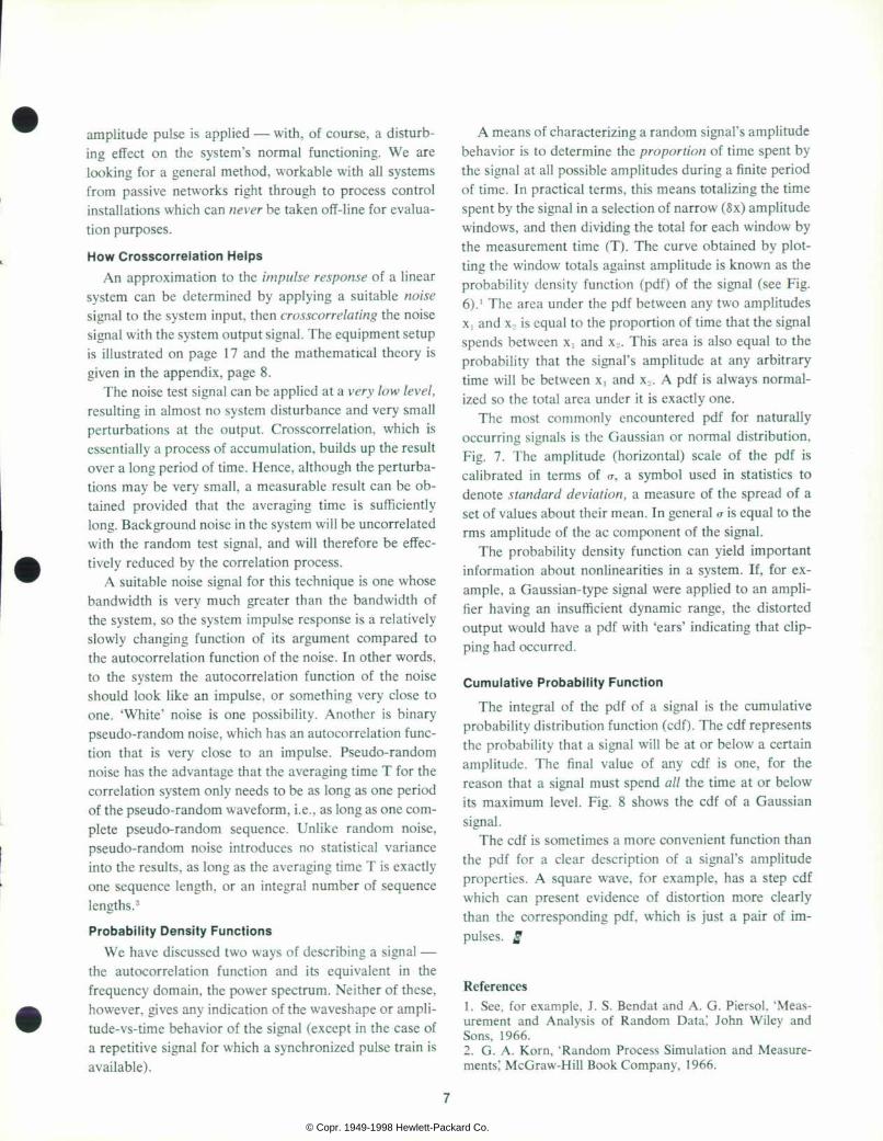
A means of characterizing a random signal's amplitude behavior is to determine the proportion of time spent by the signal at all possible amplitudes during a finite period of time. In practical terms, this means totalizing the time spent by the signal in a selection of narrow (Sx) amplitude windows, and then dividing the total for each window by the measurement time (T). The curve obtained by plot ting the window totals against amplitude is known as the probability density function (pdf) of the signal (see Fig. 6).1 The area under the pdf between any two amplitudes \i and x, is equal to the proportion of time that the signal spends between x1 and x2. This area is also equal to the probability that the signal's amplitude at any arbitrary time will be between x, and x2. A pdf is always normal ized so the total area under it is exactly one.

The most commonly encountered pdf for naturally occurring signals is the Gaussian or normal distribution, Fig. 7. The amplitude (horizontal) scale of the pdf is calibrated in terms of a, a symbol used in statistics to denote standard deviation, a measure of the spread of a set of values about their mean. In general a is equal to the rms amplitude of the ac component of the signal.

The probability density function can yield important information about nonlinearities in a system. If, for ex ample, a Gaussian-type signal were applied to an ampli fier having an insufficient dynamic range, the distorted output would have a pdf with 'ears' indicating that clip ping had occurred.

Cumulative Probabil i ty Function

The integral of the pdf of a signal is the cumulative probability distribution function (cdf). The cdf represents the probability that a signal will be at or below a certain amplitude. The final value of any cdf is one, for the reason that a signal must spend all the time at or below its maximum level. Fig. 8 shows the cdf of a Gaussian signal.

The cdf is sometimes a more convenient function than the pdf for a clear description of a signal's amplitude properties. A square wave, for example, has a step cdf which can present evidence of distortion more clearly than the corresponding pdf, which is just a pair of im pulses. S

References

1. See, for example, J. S. Bendat and A. G. Piersol, 'Meas urement and Analysis of Random Data; John Wiley and Sons, 1966. 2. G. A. Korn, 'Random Process Simulation and Measure ments! McGraw-Hill Book Company, 1966.


3. G. C. Anderson, B. W. Finnic, and G. T. Roberts, 'Pseudo- Random and Random Test Signals; Hewlett-Packard Jour nal, September 1967. 4. C. R. Trimble, 'What Is Signal Averaging?; Hewlett- Packard Journal, April 1968. 5. See, for example, M. Schwartz, 'Information Transmis sion, Modulation, and Noise; McGraw-Hill Book Company, 1 959. Or see any textbook on linear system theory.

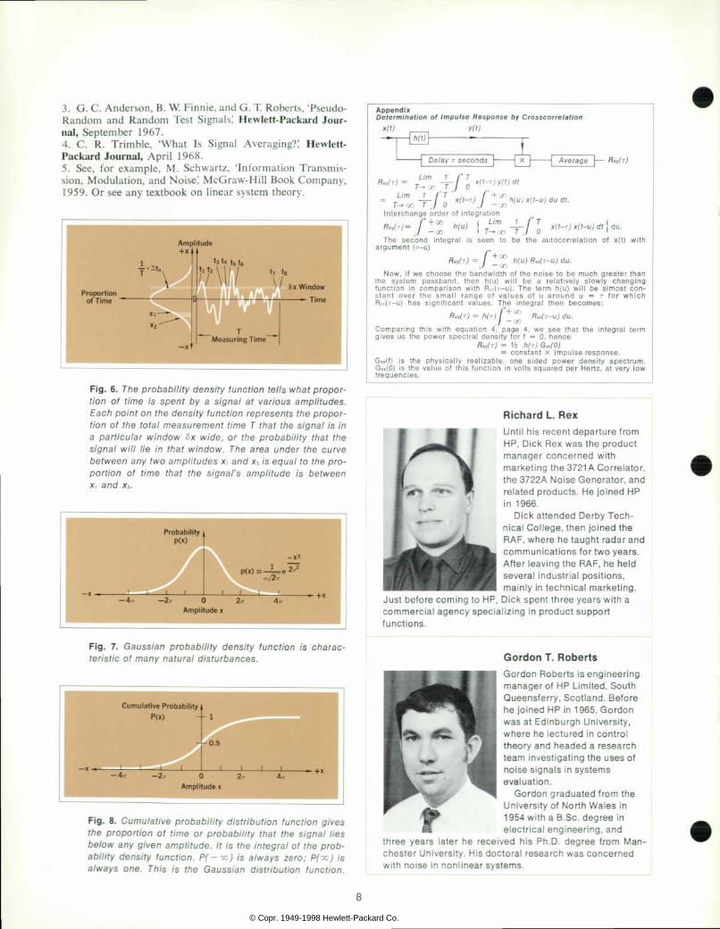
F i g . 6 . T h e p r o b a b i l i t y d e n s i t y f u n c t i o n t e l l s w h a t p r o p o r t i o n o f t i m e i s s p e n t b y a s i g n a l a t v a r i o u s a m p l i t u d e s . E a c h p o i n t o n t h e d e n s i t y f u n c t i o n r e p r e s e n t s t h e p r o p o r t i o n o f t h e t o t a l m e a s u r e m e n t t i m e T t h a t t h e s i g n a l i s i n a p a r t i c u l a r w i n d o w & x w i d e , o r t h e p r o b a b i l i t y t h a t t h e s i g n a l w i l l l i e i n t h a t w i n d o w . T h e a r e a u n d e r t h e c u r v e be tween any two amp l i t udes x , and x2 ; ' s equa l t o the p ro p o r t i o n o f t i m e t h a t t h e s i g n a l ' s a m p l i t u d e i s b e t w e e n x , and XL

F i g . 7 . G a u s s i a n p r o b a b i l i t y d e n s i t y f u n c t i o n i s c h a r a c t e r i s t i c o f many na tu ra l d i s t u rbances .

F i g . 8 . C u m u l a t i v e p r o b a b i l i t y d i s t r i b u t i o n f u n c t i o n g i v e s t h e p r o p o r t i o n o f t i m e o r p r o b a b i l i t y t h a t t h e s i g n a l l i e s b e l o w a n y g i v e n a m p l i t u d e . I t i s t h e i n t e g r a l o f t h e p r o b a b i l i t y d e n s i t y f u n c t i o n . P ( - x j i s a / w a y s z e r o ; P ( x ) i s a l w a y s o n e . T h i s i s t h e G a u s s i a n d i s t r i b u t i o n f u n c t i o n .

Appendix Determination oÃ Impulse Response by Crosscorrelation

x w y ( ' )

Delay T seconds Average â€” f in i r )

L i m 1 f T T - o o T J O

- T - l . x ( t - r ) y ( t ) d t

+ 0 0

- c o Interchange order of integrat ion

niu) x(t-u) du dt.

T h e s e c o n d i n t e g r a l i s s e e n t o b e t h e a u t o c o r r e l a t i o n o f x ( t ) w i t h argument (T-U)

f l - v W = / _ h ( u ) R , , ( T - U ) d u . Now, than we choose the bandwidth of the noise to be much greater than

t h e s y s t e m p a s s b a n d , t h e n h ( u ) w i l l b e a r e l a t i v e l y s l o w l y c h a n g i n g func t ion in compar i son w i th R , , (T -U) . The te rm h (u ) w i l l be a lmos t con s t a n t o v e r t h e s m a l l r a n g e o f v a l u e s o f u a r o u n d u = T f o r w h i c h RÂ«I(T-U) has s igni f icant va lues. The integra l then becomes:

R , V ( T ) = h ( r ) / J ' R ^ I T - U ) d u .

Compar ing th i s w i th equa t i on 4 , page 4 , we see tha t t he i n teg ra l t e rm g ives us the power spect ra l dens i ty fo r f = 0 , hence

RW(T) = ' /2 h(r ) G, , (0) = cons tan t x impu lse response.

G , i ( f ) i s t he phys i ca l l y r ea l i zab le , one s i ded power dens i t y spec t rum. GÂ«(0) is the value of this funct ion in vol ts squared per Hertz, at very low frequencies.

Richard L. Rex Unt i l h i s recen t depar tu re f rom HP , D i ck Rex was t he p roduc t m a n a g e r c o n c e r n e d w i t h market ing the 3721 A Cor re la tor , t he 3722A No ise Genera to r , and re la ted p roduc ts . He jo ined HP in 1966.

D i c k a t t e n d e d D e r b y T e c h n ica l Co l lege , then jo ined the RAF, where he taugh t radar and commun ica t i ons fo r two yea rs . A f te r leav ing the RAF, he he ld severa l indus t r ia l pos i t ions , ma in ly in techn ica l marke t ing .

Jus t be fo re coming to HP, D ick spen t th ree years w i th a commerc i a l agency spec ia l i z i ng i n p roduc t suppo r t func t ions .

Gordon T. Roberts Gordon Rober t s i s eng inee r ing manager o f HP L im i ted , Sou th Queens fe r ry , Sco t land . Be fo re he jo ined HP in 1 965, Gordon was a t Ed inburgh Un ive rs i t y , where he lec tu red in con t ro l t heo ry and headed a research team inves t iga t ing the uses o f no ise s igna ls in sys tems eva luat ion.

Go rdon g radua ted f r om the Un ivers i t y o f Nor th Wales in 1954 wi th a B.Sc. degree in e lec t r i ca l eng ineer ing , and

t h r e e y e a r s l a t e r h e r e c e i v e d h i s P h . D . d e g r e e f r o m M a n ches te r Un ive rs i t y . H i s doc to ra l resea rch was conce rned w i th no ise in non l inear sys tems.


A Calibrated Real-Time Correlator/Averager/Probabil i ty Analyzer This autocorrelation signal analyzer computes and displays 100-point autocorrelation functions,

c rossco r re la t i on func t i ons , waveshapes o f s igna ls bu r ied i n no i se , p r o b a b i l i t y d e n s i t y f u n c t i o n s , a n d p r o b a b i l i t y d i s t r i b u t i o n s .

By George C. Anderson and Michael A. Perry

EVER SINCE THE THEORY OF CORRELATION WAS DE VELOPED and the potential advantages of the technique brought to light, people have been looking for practical ways to apply it. Because correlation requires prodigious computation, a common way of getting correlation func tions has been to record data and process them later, off line, in a digital computer. The problem with this method is that it takes too much time. If the data are inadequate or if procedures or programs need modification, it takes a long time to find out. In the meantime, a lot of equip ment may be tied up.

On-line correlation has the advantage of providing answers where they are needed, that is, where the meas urements are being made. But while it isn't unknown, on-line correlation isn't very common, either, the reason being that instruments that can correlate in real time haven't been very accurate, versatile, or easy to use.

The HP Model 3 721 A Correlator, Fig. 1, is designed to be a truly practical way of getting correlation functions in real time. This new instrument processes analog signals â€” on line and in real time - â€” and presents the results on

a calibrated CRT display. It is more than just a corre lator; it has two analog inputs and it can compute â€¢ the autocorrelation function of one input signal â€¢ the crosscorrelation between two signals â€¢ the probability density function of an input signal, or

its integral, the probability distribution â€¢ the waveshape of a repetitive signal buried in noise

(by signal recovery or signal averaging).

â€¢ The averaging 'averaging' has two meanings in th is art ic le. Signal averaging is a tech n i q u e o f ( s e e a n a l y s i s ; i t i s u s e f u l f o r r e c o v e r i n g r e p e t i t i v e s i g n a l s f r o m n o i s e ( s e e r e f e r e n c e 1 ) . A v e r a g i n g i s a m a t h e m a t i c a l p r o c e s s ; i t i s u s e d i n a l l o f t h e m o d e s o f opera t ion o f the new co r re la to r : au toco r re la t i on , c rosscor re la t i on , p robab i l i t y d i sp lay , a n d s i g n a l a v e r a g i n g . T o a v o i d c o n f u s i o n w e w i l l o f t e n r e f e r t o s i g n a l a v e r a g i n g a s ' s igna l recovery . '

In general, using the new correlator is similar to using an oscilloscope, and in some ways, it is easier to use than an oscilloscope. It has a wide selection of measurement parameters â€” sampling rates, averaging times, and so on â€” and the vertical scale factor of the display, which is

affected by several of these selectable parameters, is auto matically computed and displayed on the front panel. Like an oscilloscope, and unlike off-line computers, the correlator can follow slowly varying signals, can give a 'quick-look' analysis to show the need for and the results of adjustments, and can easily be carried from place to place (it weighs 45 pounds).

Digital Techniques Used

Model 3721 A is primarily a digital instrument, al though it does use some analog techniques. Long-term stable averaging, which is necessary for the very-low- frequency capability, can only be done digitally; capac- itive averaging, which is used in some correlators, simply can't provide long enough time constants with capacitors of reasonable size. A simple, accurate, and stable digital multiplier which is fast enough to allow sampling rates up to 1 MHz is another benefit of digital operation.

Model 3721A displays the computed function on its CRT using 100 points. Typical correlation displays are shown in Fig. 2.

100 points are sufficient for many measurements; how ever, if more resolution is required, there is an option (for the correlation mode) which provides additional delay in batches of 100 points, up to a maximum of 900 points. Using this pre-computational delay, the time scale can be compressed and the correlation function examined one section at a time.


Â«ÃTHÂ»

] R E S E T K â € ž

Fig. easy oscil loscope. its versati l i ty, Model 3721 A Correlator is as easy to use as an oscil loscope. A n i l l u m i n a t e d p a n e l s h o w s t h e d i s p l a y s e n s i t i v i t y i n V ' / c m f o r c o r r e l a t i o n a n d i n V / c m f o r s i g n a l a v e r a g i n g ( s i g n a l r e c o v e r y ) . T h e c o r r e l a t o r h a s a w i d e s e l e c t i o n o f m e a s u r e m e n t p a r a m e t e r s a n d m o d e s o f o p e r a t i o n , i n c l u d i n g a ' q u i c k - l o o k ' m o d e w h i c h m i n i m i z e s d e l a y s

i n s e t t i n g u p e x p e r i m e n t s .

(a)

F i g . a n d t i m e o f 1 0 0 - p o i n t c o r r e l a t i o n f u n c t i o n s c o m p u t e d a n d d i s p l a y e d i n r e a l t i m e b y Mode l 3721 A Cor re la to r . (See a lso page 20 fo r au tocor re la t ion func t ions o f speech sounds . ) ( a ) A u t o c o r r e l a t i o n f u n c t i o n o f 1 5 - b i t p s e u d o - r a n d o m b i n a r y s e q u e n c e , c l o c k p e r i o d 5 m s .

T i m e s c a l e 1 m s / m m . ( b ) C r o s s c o r r e l a t i o n b e t w e e n n o i s e i n a m a c h i n e s h o p a n d n o i s e f r o m a n e a r b y v e n t i l a t i n g

f a n . D o u b l e h u m p i n c e n t e r s h o w s t h e r e a r e t w o p r i n c i p a l t r a n s m i s s i o n p a t h s f r o m f a n to mach ine shop , d i f f e r i ng i n p ropaga t ion de lay by 4 ms .

10


The horizontal axis of the display is scaled ten points to each centimeter and is calibrated in time per milli meter. The time per millimeter is also the period between successive samples of the analog input. The 'sweep rate' can be switched from 1 /^s/mm to 10 s/mm. It is con trolled by a crystal clock and is accurate within 0.1%. Lower sweep rates may be provided by inputs from an external source.

The vertical axis is accurately calibrated, and an illuminated display beside the CRT avoids the 'numbers trouble' which can easily occur in an instrument which uses both analog and digital techniques. The vertical scale factor of the display depends upon the product of four numbers. These are the settings of the two analog input amplifiers, a gain control for the averaging algorithm, and a control which expands the trace in the vertical axis. The first two variables follow a 1, 2, 4, 10 sequence, the third follows a 1, 10, 100 sequence, and the fourth fol lows a binary progression. The scale factor is also affected by the function the instrument is performing. Autocorre lation requires the square of one analog channel gain set ting, whereas crosscorrelation requires the product of two. Signal recovery and probability display have entirely different requirements. All of this might leave the user with some awkward mental arithmetic, were it not for the illuminated display, which shows the scale factor.

* T h e s i n c e o f a s t a t i s t i c a l a n a l y z e r i s d i f f i c u l t t o d e f i n e , s i n c e t h e a c c u r a c y o f the d isp layed resu l t depends upon the s ta t is t ics and bandwidth o f the input s igna ls and on the cor re la to r t ime cons tan t used . Sys temat ic e r ro rs in the new cor re la to r â€” such th ings as d i sp lay non l i nea r i t y and va r ia t i ons i n quan t i ze r ga in ( see append ix ) â€ ” a re t yp i ca l l y l e ss t han 1 o r 2 pe r cen t a t l ow f r equenc ies .

Being a digital instrument, the correlator is easily in terfaced with a computer; there is a plug-in option for this purpose. There are also rear-panel outputs for an X-Y recorder.

How It Correlates

The equation for the crosscorrelation function of two waveforms a(t) and b(t) which are both functions of time is Rha(T) = a(t)b(t-r) where the bar denotes taking an average. There are three important operations: delaying b(t) by an amount T, mul tiplying the delayed b(t) by the current value of a(t), and taking the average value of these products over some time interval. The correlation function is a plot of Rba(r) versus the delay, T. The new correlator computes 100 values of the correlation function for 100 equally spaced values of T and does them simultaneously, as follows.

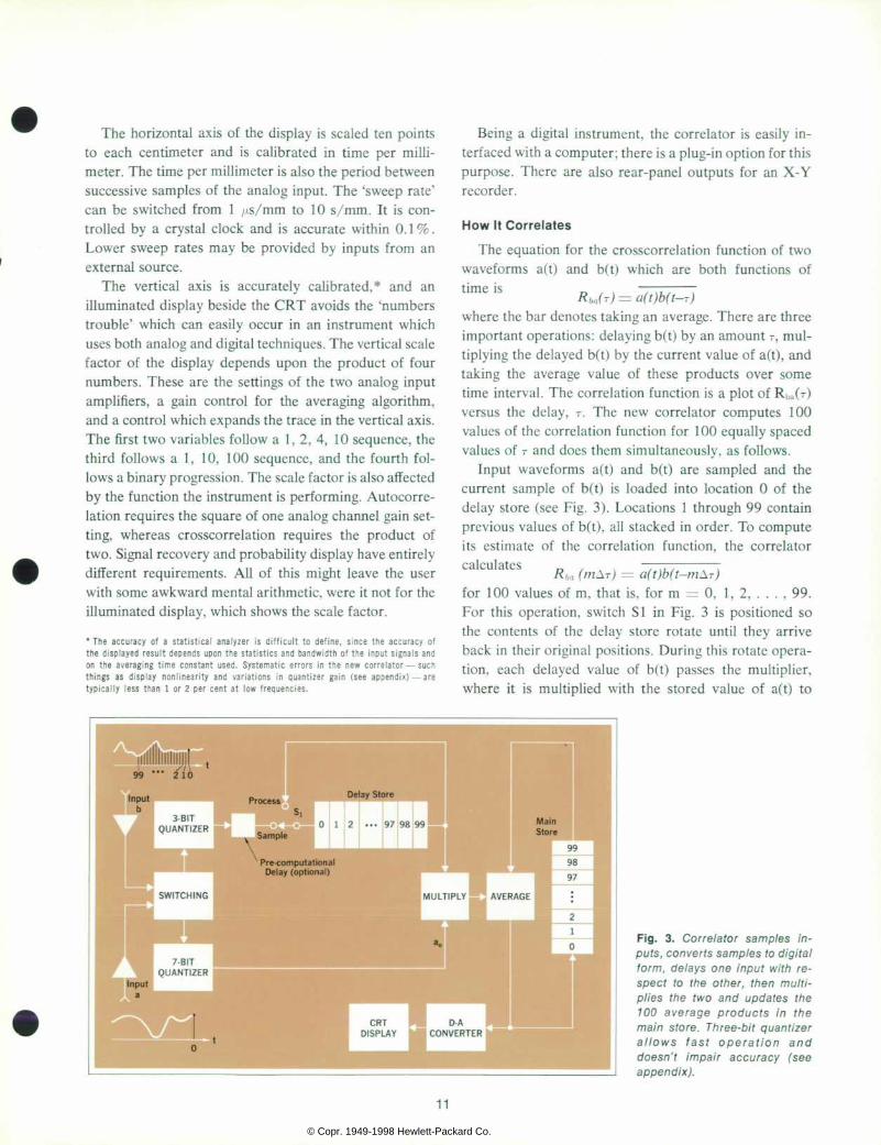
Input waveforms a(t) and b(t) are sampled and the current sample of b(t) is loaded into location 0 of the delay store (see Fig. 3). Locations 1 through 99 contain previous values of b(t), all stacked in order. To compute its estimate of the correlation function, the correlator calculates

for 100 values of m, that is, for m = 0, 1,2,. . . , 99. For this operation, switch SI in Fig. 3 is positioned so the contents of the delay store rotate until they arrive back in their original positions. During this rotate opera tion, each delayed value of b(t) passes the multiplier, where it is multiplied with the stored value of a(t) to

F i g . 3 . C o r r e l a t o r s a m p l e s i n pu ts , conver ts samples to d ig i ta l f o r m , d e l a y s o n e i n p u t w i t h r e s p e c t t o t h e o t h e r , t h e n m u l t i p l i e s t h e t w o a n d u p d a t e s t h e 1 0 0 a v e r a g e p r o d u c t s i n t h e m a i n s t o r e . T h r e e - b i t q u a n t i z e r a l l o w s f a s t o p e r a t i o n a n d d o e s n ' t i m p a i r a c c u r a c y ( s e e append ix ) .

11


produce a series of 1 00 products a(t)b(t-mAT). The prod ucts are fed into an averager where they interact with the contents of the serial main store, which are also under going a rotate operation. The contents of the main store are the 100 previously calculated values of Rta(mAT). In the averager, the new product a(t)b(t) updates Rhil(0), the product a(t)b(tâ€” AT) updates Rba(AT), and so on up to Rba(99AT). The main store, therefore, always contains the most recent estimate of the correlation function. A complete sequence of rotation, multiplication, and av eraging is known as a process cycle. When it is complete, the instrument reverts to a data acquisition cycle and new samples of a(t) and b(t) are taken. The new value of b(t) is put into location 0 of the delay store, and all others are shifted down one place. b(tâ€” 99Ar) 'rolls off the end' and is discarded, since it is of no further value. When pre- computational delay is needed, it is added by increasing the length of the delay store.

The time taken up by a process cycle is 135.6 /.is, the cycle time of the main store. How then, you may ask, can the instrument operate with a sampling rate as high as 1 MHz, yet enter a process cycle after each sample has been taken? The answer lies in the assumption that the input signals are stationary; this is a way of saying that the statistics of the signals are constant for all time. When this is true, we can wait as long as we wish between suc cessive data samples without affecting the accuracy of the measurement, as long as we take enough samples even tually.

At high data sampling rates (AT < 333 /Â¿s) the cor relator operates in an ensemble sampling mode, or batch mode (see Fig. 4). In the batch mode, instead of entering one new sample of b(t) into the delay store at the instant a(t) is sampled, the sampling of a(t) is preceded by taking 99 fresh samples of b(t) and entering those into the delay store first. * We now have stored information showing the relationship between a(t) and 1 00 consecutive samples of b(t) as before, but now the speed with which data can be acquired is independent of the time taken for a process cycle. There is a tradeoff involved in batch sampling. For statistical accuracy, a large number of samples of a(t) must be taken, and this makes the measurement less effi cient than the normal mode which was described first. However, batch sampling is only used at high sampling rates where the extra real time involved is too small to be significant in many cases.

* F o r b y = 1 , 3 . 3 3 , o r 1 0 / i s , 9 9 s a m p l e s o f b ( t ) a r e t a k e n , f o l l o w e d b y s i m u l t a n e o u s samp l ing o f a ( t ) and b ( t ) . Fo r \T = 33 .3 o r 100 /Â ¡s , on ly 9 samp les o f b ( t ) p recede the s i m u l t a n e o u s s a m p l i n g o f a ( t ) a n d b ( t ) . F o r \ T > 3 3 3 ^ s , a ( t ) a n d W t ) a r e a l w a y s samp led s imu l taneous ly , i . e . , the ins t rument opera tes in the norma l mode .

Signal Recovery

It is the batch mode of operation which allows the Model 3721 A Correlator to perform signal averaging or signal recovery. In this case, there is no signal a(t). A constant value is inserted into the a(t) storage register and, on receipt of a sync pulse, 100 sampled values of b(t), the signal being averaged, are entered into the delay store. A process cycle rotates the delay store and updates the information in the main store. Since the delay store has a much faster access time than the main store, this method of operation allows fast sampling at rates inde pendent of the main-store cycle time.

Two Averaging Modes

Two kinds of averaging are available for correlation, probability measurements, or signal recovery. A front- panel switch selects one or the other.

One averaging mode is straightforward summation. The function computed after N samples of the inputs have been taken at intervals of AT, starting at t = 0, is

j N + m-1

N k = m

where m = 0, 1, 2, . . ., 99. For signal averaging, or sig nal recovery, a(kAr) is held constant, while for correla tion it varies with the input a(t).

The second averaging mode is a running average which forgets very old information. If AN_a is the current value of the running average and a new input IN- arrives, the new average would be

A l f = A y - 1 + ' N

where N is the number of samples that has been taken. Because it is difficult to divide by an arbitrary integer N at a reasonable cost in a high-speed system, the new cor relator divides by the nearest power of 2, so it can divide simply by shifting. The algorithm becomes

AN = AN.Â¡ IN â€”

2Â»

No error is introduced into the averages by dividing by 2n instead of by N ; the averages just take a little longer to approach within a given percentage of their final values (assuming these final values aren't changing).2

The running-average algorithm acts like an RC aver aging circuit; the output responds exponentially to a step input with a time constant approximately equal to 2nAT seconds. A powerful feature of this exponential averaging algorithm is the effect of the varying value of n during the measurement. Initially, n is zero. Then, as the meas-

12


urement proceeds, N, the number of samples, becomes equal to the next higher value of 2", and n is incremented. This has the effect of averaging with a variable capacitor C whose value is initially small, and becomes larger as the measurement proceeds. High-frequency noise is aver aged out immediately, leaving the lower frequencies for later and giving a rapid preliminary estimate of the cor relation function or average. Once n has reach the ter minal value determined by the front-panel time-constant switch, the system continues to operate with that time constant. A wide range of control over the value of n provides the user with a useful and flexible averaging capability.

Details of Operation

Figs. 3 and 5 together show the correlator's block diagram. Analog signals are scaled by two preamplifiers and fed into a changeover switching network, which routes signals into the reference or delay channels ac cording to the function chosen by a front-panel switch. Next, the signals are digitized or quantized. The reference signal is converted into a seven-bit, two's complement code by a ramp-and-counter-type analog-to-digital con verter whose conversion time has a maximum value of 42 /is. The signal which is to be delayed with respect to the reference signal is fed into a fast ( < 1 /is) three-bit converter which has a special encoding characteristic (see Fig. 6). Rigorous computer analysis showed that the coarseness of the three-bit encoding law would not impair the accuracy of the correlator. The choice of a three-bit * See the appendix, page 15.

F i g . 4 . F o r d e l a y i n c r e m e n t s \ T ( t i m e / m m ) o f 3 3 3 u s o r m o r e , t h e c o r r e l a t o r o p e r a t e s i n t h e n o r m a l m o d e , g o i n g t h rough a p rocess cyc le â€ ” upda t i ng t he WO s to red ave r age p roduc ts â€” a f te r each sample o f the inpu ts i s taken . F o r s h o r t e r d e l a y i n c r e m e n t s , t h e c o r r e l a t o r u s e s t h e b a t c h m o d e , t a k i n g 1 0 0 s a m p l e s o f i n p u t b t o r e a c h s a m p l e o f i n p u t a . A l t h o u g h m u c h s l o w e r , t h e b a t c h m o d e i s u s e d o n l y a t v e r y s h o r t d e l a y i n c r e m e n t s a n d i s n ' t a p rac t i ca l l im i t a t i on .

F i g . 5 . T h e a r i t h m e t i c u n i t c o m p u t e s a v e r a g e s d i g i t a l l y , s o i t d o e s n ' t h a v e t h e s t a b i l i t y p r o b l e m s o f c a p a c i t i v e a v e r a g i n g . Mu l t i p l i ca t ions and d iv i s ions , a l l b y p o w e r s o f t w o , r e q u i r e o n l y t ime sh i f ts .

13


code for the delay channel made it possible to provide a fast encoder at relatively low cost, and to keep the ca pacity of the delay store to a minimal 300 bits.

In the three-bit encoder the signal is coarsely quan tized into values of 0, Â±1, Â±2, or Â±4. The virtue of this simple law is that to multiply the quantized output by another binary word involves only shift operations; this saves hardware in the multiplier.

The current estimate of the correlation function (or average) is stored serially in 100 24-bit words in the main store, which is a glass ultrasonic delay line having a ca pacity of 102 24-bit words. The two extra words are used for bookkeeping and control. Information in the main store recirculates at a bit rate of approximately 18 MHz, one complete cycle taking about 135.6 /is. Operation of the glass delay line is similar to shouting down a long tunnel, catching the sound at the other end, and feeding it back to the beginning.

All arithmetic processing is carried out on the output of the main store using two's complement arithmetic. Subtraction is done by a 'two's complement and add' algorithm. Multiplications and divisions are all by powers of two, so they are implemented as time delays and time advances, respectively.

Display

Output from the memory to the display is via the shift register called the 'main store window! For each of the 100 computed points, eight bits from this register are transferred to a buffer register, converted to analog form, and used to position the CRT beam vertically. The hori zontal position of each dot is determined by a counter. Which eight of the 24 possible bits are displayed depends on the display gain setting, which has three values.

Probabil ity Distributions

The measurement of probability density and probabil ity distribution functions depends for its operation upon the constant cycle time of the main store. When the first word in the chain emerges from the main store, the input signal is sampled at the input to the seven-bit ramp-and- counter A-D converter. This time we are not concerned with converting the sampled voltage into binary code, but into a time delay. The sampling instant initiates a ramp which runs down linearly from the value of the sampled input signal to a reference voltage. When co incidence occurs, information is gated into adder Al to increment the word which is currently in the arithmetic unit. In the probability density mode, no further words are incremented; but in the probability distribution mode, which is the integral of the density, all succeeding words are also incremented. The averaging algorithms operate as before. An example of a probability display is shown in Fig. 7.

F i g . 7 . P r o b a b i l i t y d e n s i t y f u n c t i o n o f s i n e w a v e p l u s G a u s s i a n n o i s e . M o d e l 3 7 2 1 A C o r r e l a t o r c a n a l s o c o m p u t e t h e c u m u l a t i v e d i s t r i b u t i o n f u n c t i o n , w h i c h i s t h e i n t e g r a l o f t h e p r o b a b i l i t y d e n s i t y f u n c t i o n .

Acknowledgments

The feasibility studies for the Model 3721 A Corre lator were initiated by Brian Finnie. Associated with us in the electronic design were Glyn Harris, Alister Mc- Parland, David Morrison, Rajni Patel, and John Picker ing. Peter Doodson did the industrial design. Product design was by Duncan Reid and David Heath. Jerry Whitman assisted with the feasibility studies, g

F i g . 6 . T h e t h r e e - b i t q u a n t i z e r ' s o u t p u t s a r e p o w e r s o f t w o . M u l t i p l i c a t i o n b y t h e m i s s i m p l y a g a t i n g f u n c t i o n .


References

1. C. R. Trimble, 'What Is Signal Averaging?; Hewlett- Packard Journal, April 1968. 2. J . E. Deardorff and C. R. Trimble, 'Calibrated Real- Time Signal Averaging! Hewlett-Packard Journal, April, 1968.

Appendix: Equivalent Gain of a Quantizer

A q u a n t i z e r o r a n a l o g - t o - d i g i t a l c o n v e r t e r i s a n o n l i n e a r d e v i c e w h i c h h a s a s t a i r c a s e c h a r a c t e r i s t i c l i k e t h e o n e s h o w n i n F i g . 6 , p a g e 1 4 . Q u a n t i z a t i o n h a s t h e e f f e c t o f a d d i n g d i s t o r t i o n i n t h e f o r m o f ' c o r n e r s ' t o a n i n p u t s i g n a l x ( t ) . Th i s d i s to r t i on , ca l l ed quan t i za t i on no ise , can be shown t o b e i s w i t h t h e i n p u t s i g n a l . I f t h e q u a n t i z e r i s assumed to be su f f i c i en t l y w ideband no t t o d i s to r t t he s igna l i n o the r ways , i t s ou tpu t w i l l have a componen t p ropo r t i ona l t o t h e i n p u t s i g n a l , K x ( t ) , p l u s u n c o r r e l a t e d q u a n t i z a t i o n n o i s e , n ( t ) . T h e c o n s t a n t K i s c a l l e d t h e e q u i v a l e n t g a i n o f t he quan t i ze r .

I t has been known fo r some t ime tha t accu ra te co r re l a t i on m e a s u r e m e n t s c a n b e m a d e u s i n g v e r y c o a r s e q u a n t i z a t i o n o f da ta , i . e . , ve ry few b i t s . Cor re la t ion invo lves an averag ing p r o c e s s , s o a c o r r e l a t o r i s o n l y a f f e c t e d b y t h e a v e r a g e d r e s p o n s e o f t h e q u a n t i z e r t o a n i n p u t s i g n a l . T h i s a v e r a g e d r e s p o n s e i s t h e e q u i v a l e n t g a i n K . F o r a c c u r a t e c o r r e l a t i o n m e a s u r e m e n t s , K s h o u l d b e c o n s t a n t o v e r t h e s p e c i f i e d r a n g e o f s i g n a l a m p l i t u d e s . T h e c u r v e b e l o w i s t h e e q u i v a len t ga in o f the th ree-b i t quant izer used in the Mode l 3721 A C o r r e l a t o r , f o r a G a u s s i a n i n p u t s i g n a l . T h e s h a r p d r o p i n g a i n a t l o w s i g n a l l e v e l s o c c u r s b e c a u s e t h e s i g n a l b a r e l y c l imbs ove r t he f i r s t s tep o f t he quan t i ze r ' s s ta i r case cha rac t e r i s t i c . T h i s d e f e c t i s o v e r c o m e b y a d d i n g u n c o r r e l a t e d G a u s s i a n n o i s e t o t h e i n p u t s i g n a l , t h e r e b y k e e p i n g t h e e q u i v a l e n t g a i n n e a r l y c o n s t a n t d o w n t o z e r o i n p u t . T h e f a l l o f f i n g a i n a t h i g h s i g n a l l e v e l s c a n b e a t t r i b u t e d t o saturat ion.

T h e f a c t t h a t a c c u r a t e c o r r e l a t i o n m e a s u r e m e n t s c a n b e m a d e u s i n g o n l y a t h r e e - b i t q u a n t i z e r i s s i g n i f i c a n t . I n t h e c a s e o f t h e M o d e l 3 7 2 1 A C o r r e l a t o r , i t m e a n s r e d u c e d c o m p lex i t y and cos t , and h ighe r speed .

* D . G . Wa t t s , 'A S tudy o f Amp l i t ude Quan t i sa t i on w i t h App l i ca t i on t o Co r re la t i on Determinat ion,1 Ph.D. Thesis, Univers i ty of London, January 1962.

Norma l i zed rms Inpu t S igna l (Vo l t s )

Michael A. Perry

Mike Per ry s tud ied e lec t ron i c eng ineer ing a t the Un ivers i t y Co l lege o f Nor th Wa les , ob ta in ing the B .Sc . (Honours ) degree in 1963 and the Ph.D. degree in 1966. H is doc tora l research was i n e lec t rome te r measuremen t techn iques , and

k , a p a p e r h e c o - a u t h o r e d I o n t h i s r e s e a r c h w o n a n I E E

^ E l e c t r o n i c s D i v i s i o n p r e m i u m fo r 1965. A f te r jo in ing HP

t i n 1 9 6 6 , M i k e w o r k e d o n t h e 3722A No ise Genera to r and the 3721A Cor re la to r . He i s now invo lved in new p roduc t i nves t iga t ions .

George C. Anderson G e o r g e A n d e r s o n w a s p r o j e c t leader on the 3722A No ise Genera to r and on the 3721A Cor re la to r . He has been wi th HP s ince 1966.

Geo rge g radua ted f r om Her io t -Wat t Un ive rs i t y , Ed inburgh , in 1954 . A f te r comp le t i ng a two -yea r g radua te course in e lec t r i ca l eng ineer ing , he d id va r ied indus t r ia l work fo r a number o f years . Dur ing the th ree years p r io r to h is jo in ing HP,

he was w i th the Roya l Observa to ry , Ed inburgh , where he deve loped da ta record ing sys tems fo r the se ismo logy un i t .

15


S P E C I F I C A T I O N S HP Model 3721A

Correlator I N P U T C H A R A C T E R I S T I C S Two separate input channels , A and B, w i th ident ica l ampl i f ie rs .

B A N D W I D T H : T h e B i n p u t s i g n a l i s s a m p l e d a t a m a x i m u m r a t e o f 1 MHz . Acco rd ing t o t he samp l i ng t heo rem, t h i s means t ha t i npu t s i g n a l s m u s t b e b a n d - l i m i t e d t o 5 0 0 k H z o r l e s s . A u s e f u l r u l e o f thumb cycle random signals is to al low at least four samples per cycle o f t he upper 3 -dB cu to f f f r equency ; t hus the max imum 3 -dB cu to f f f r e q u e n c y w o u l d b e 2 5 0 k H z . P u r e s i n e - w a v e i n p u t s w o u l d p r o b ab ly requ i re more samples per cyc le to g ive a recogn izab le p ic tu re o n t h e C R T ; h o w e v e r , f o r c o m p u t e r p r o c e s s i n g o f t h e d a t a f o u r samples per cyc le would be ent i re ly adequate. Model 3721A's lower cu to f f f requency i s se lec tab le , dc o r 1 Hz .

INPUT RANGE: 6 ranges, 0.1 V rms to 4 V rms, in 1, 2, 4, 10 sequence. ANALOG-TO-DIGITAL CONVERSION: F ine quan t i ze r ; 7 b i t s . Coarse

quantizer ( feeds delayed channel): 3 bi ts. Coarse quantizer l inearized by internal ly-generated wideband noise (d i ther) .

OVERLOAD: Maximum permiss ib le vo l tage a t input : dc coupled 120 V peak , ac coup led 400 V = dc + peak ac .

INPUT IMPEDANCE: Nominal ly 30 pF to ground, shunted by 1 MS!. CORRELATION MODE

Simul taneous computat ion and d isp lay of 100 va lues of auto or cross- c o r r e l a t i o n f u n c t i o n . D i s p l a y s e n s i t i v i t y i n d i c a t e d d i r e c t l y i n W c m o n i l l um ina ted pane l . Non-des t ruc t i ve readou t ; compu ted func t i on can be d isp layed for an un l imi ted per iod wi thout deter iora t ion. (Non-permanent s torage; data c leared on swi tchof f . )

T IME SCALE: (T ime/mm = de lay incrementA^) 1 / i s to 1 second ( to ta l de lay span 100 iÂ¿s to 100 seconds) in 1 , 3 .33 , 10 sequence w i th in ternal c lock. Other de lay increments wi th external c lock; min imum increment 1 #s (1 MHz), no upper l imi t .

DELAY OFFSET: Opt ion ser ies 01 prov ides de lay o f fse t (p recomputa- t ion represents faci l i ty. Without offset, f irst point on display represents zero delay; wi th of fset , delay represented by f i rs t point is selectable f rom 100 AT to900 AT i n mu l t i p l es o f 100 AT .

DISPLAY SENSITIVITY: 5 x 10-<>W/cm to 5 Wcm. Cal ibrat ion automat ica l ly d isp layed by i l luminated panel .

VERT ICAL RESOLUTION: Depends on d i sp l ay sens i t i v i t y . M in imum resolut ion Â¡s 25 levels/cm. Interpolat ion fac i l i ty connects points on display.

AVERAGING: Two modes a re p rov ided : Summat ion ( t rue ave rag ing ) and Exponent ial . 1 . S U M M A T I O N M O D E

Computa t ion au tomat ica l l y s topped a f te r N p rocess cyc les , a t which t ime each point on the d isp lay represents the average of N products . N is se lec tab le f rom 128 to 128 x 1024 (2 ' to 2" in b inary s teps) . D isp lay ca l ib ra t ion automat ica l ly normal ized for a l l va lues of N. Summat ion t ime indicated by i l luminated panel .

2 . E X P O N E N T I A L M O D E Dig i ta l equ iva len t o f RC averag ing , w i th t ime cons tan t se lec t able from 36 ms to over 10' seconds. Approximate t ime constant ind ica ted by I l lumina ted pane l . D isp lay cor rec t l y ca l ib ra ted a t a l l t imes dur ing the averag ing process.

SIGNAL RECOVERY MODE (Channel B only) Detects coherence Â¡n repeated events, when each event is marked by a

synchron iz ing pu lse . A f te r each sync pu lse , a ser ies o f 100 samples o f channe l B inpu t i s taken , and cor respond ing samp les f rom each ser ies are averaged. The 100 averaged samples are d isp layed s imul taneous ly . D isp lay sens i t iv i ty is ind icated d i rec t ly in V/cm on i l luminated panel .

S Y N C H R O N I Z A T I O N : A n a v e r a g i n g s w e e p Â ¡ s i n i t i a t e d e i t h e r b y a t r igger pulse from an external source (EXT) or, in internal ly t r iggered mode ( INT) , by a pu lse de r i ved f rom the in te rna l c lock . In the INT mode, the s tar t o f each sweep Â¡s marked by an output pu lse (s t im ulus) used to synchronize some external event .

TRIGGER INPUT: Averaging sweep in i t iated by negat ive-going step. STIMULUS OUTPUT: Negat ive-going pulse at start of averaging sweep. TIME SCALE: (T ime/mm = in terval between samples) 1 / /s to 1 second

( to ta l d isp lay width 100 AS to 100 seconds) in 1 , 3 .33, 10 sequence wi th in ternal c lock. Other in tervals (hence other d isplay widths) wi th external c lock; minimum interval 1 MS (1 MHz), no upper l imi t .

DISPLAY SENSITIVITY: 50 i iV/cm to 1 V/cm. Cal ibrat ion automat ica l ly d isplayed by i l luminated panel .

VERTICAL RESOLUTION: Depends on d i sp lay sens i t i v i t y . M in imum resolut ion Â¡s 25 levels/cm. Interpolat ion fac i l i ty connects points on display.

SIGNAL ENHANCEMENT: Improvement in s ignal - to-no ise ra t io equals square root of number of averaging sweeps.

NUMBER OF SWEEPS = N Â¡n summat ion mode; N x gain factor of 1 , 10 or 100 in exponent ial mode.

PROBABILITY MODE (Channel A only) D isp lays e i ther (1 ) ampl i tude probab i l i t y dens i ty func t ion (pd f ) o r (2 ) integral of the pdf of channel A input . Signal ampl i tude represented by hor izonta l d isp lacement on d isp lay , w i th zero vo l ts a t center ; ver t ica l d isplacement represents ampl i tude probabi l i ty . DISPLAY SENSITIVITY: Hor izontal sensi t iv i ty 0.05 V/cm to 2 V/cm Â¡n

5, 10, 20 sequence. HORIZONTAL RESOLUTION: 100 discrete levels Â¡n 10 cm wide display

= 10 leve ls /cm. VERTICAL RESOLUTION: 256 d isc re te leve ls in 8 cm h igh d isp lay =

32 levels/cm. VERTICAL SCALING: Depends on averaging method used (summat ion

or exponent ial) . SAMPLING RATE: 1 Hz to 3 kHz Â¡n 1 , 3 , 10 sequence w i th in te rna l

c lock. Other sampl ing rates wi th external c lock; maximum frequency 3 kHz, no lower f requency l imi t .

I N T E R F A C I N G X-Y RECORDER: Separate analog outputs corresponding to hor izontal

and vert ical coordinates of the CRT display. OSCILLOSCOPE: Separa te ana log ou tpu ts cor respond ing to the hor i

zontal and vert ical coordinates of the CRT display. NOISE GENERATOR MODEL 3722A: Control of the Correlator f rom the

Mode l 3722A Noise Genera tor . The gate s igna l f rom the 3722A Â¡s used to set the Correlator into RUN state; on terminat ion of the gate signal, Correlator wi l l go into HOLD state.

DIGITAL COMPUTER: Opt ion 020 prov ides in ter face hardware (buf fer card) for reading out d isplayed data to d ig i ta l computer .

C L O C K INTERNAL CLOCK: A l l t im ing s igna ls der ived f rom crys ta l -cont ro l led

o s c i l l a t o r : s t a b i l i t y 4 0 p p m o v e r s p e c i f i e d a m b i e n t t e m p e r a t u r e range.

EXTERNAL CLOCK: Maximum frequency 1 MHz. PROCESS CLOCK: 135 ILS wide negative-going pulse. Normally +12 V,

fa l ls to 0 V at s tar t o f each process cyc le and returns to +12 V af ter 135 MS.

REMOTE CONTROL & INDICATION CONTROL: Remote control inputs for RUN, HOLD and RESET funct ions

are connected to DATA INTERFACE socket on rear panel . INDICATION: Remote ind ica t ion o f co r re la to r RUN, HOLD or RESET

states is avai lable at the DATA INTERFACE socket on rear panel . GENERAL

AMBIENT TEMPERATURE RANGE: 0Â° to + 50Â°C. POWER: 115 or 230V Â±10%, 50 to 1000 Hz, 150 W. DIMENSIONS: 16% in. wide, 10% in. h igh, 18% in. deep overal l (426 x

273 x 476 mm). WEIGHT: 45 Ib. (20.5 kg) net.

OPTIONS DELAY OFFSET OPTION SERIES 01

Option 011 Correlator with 100 At offset faci l i ty. Option 013 Correlator with 300 At offset faci l i ty. Option 015 Correlator with 500 At offset faci l i ty. Option 017 Correlator with 700 At offset faci l i ty.

The above opt ions are extendable ( factory convers ion only) to 900 At offset, in mult iples of 200 At. Option 019 Correlator with 900 At offset faci l i ty.

DATA INTERFACE: Option series 02 Opt ion 020 Corre lator wi th in ter face for data output to computer .

PRICE: Model 3721A, $8350.00

MANUFACTURING DIVISION: HEWLETT-PACKARD LTD. South Queensferry West Loth ian, Scot land

16


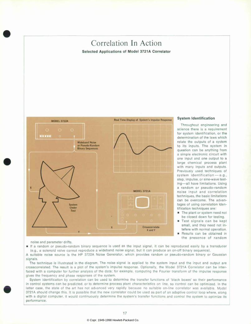
Correlation In Action Selected Appl icat ions of Model 3721A Corre la tor

System Identif ication T h r o u g h o u t e n g i n e e r i n g a n d

s c i e n c e t h e r e i s a r e q u i r e m e n t f o r s y s t e m i d e n t i f i c a t i o n , o r t h e de te rm ina t i on o f t he l aws wh i ch r e l a t e t h e o u t p u t s o f a s y s t e m t o i t s i n p u t s . T h e s y s t e m i n q u e s t i o n c a n b e a n y t h i n g f r o m a s i m p l e e l e c t r o n i c c i r c u i t w i t h o n e i n p u t a n d o n e o u t p u t t o a l a r g e c h e m i c a l p r o c e s s p l a n t w i t h m a n y i n p u t s a n d o u t p u t s . P r e v i o u s l y u s e d t e c h n i q u e s o f s y s t e m i d e n t i f i c a t i o n â € ” e . g . , s tep , impu lse , o r s ine -wave tes t ing â€” al l have l imi tat ions. Using a r a n d o m o r p s e u d o - r a n d o m n o i s e i n p u t a n d c o r r e l a t i o n techn iques , the bas ic l im i ta t ions c a n b e o v e r c o m e . T h e a d v a n t a g e s o f u s i n g c o r r e l a t i o n i d e n t i f i ca t i on t echn iques a re : â€¢ The plant or system need not

b e c l o s e d d o w n f o r t e s t i n g . â € ¢ T e s t s i g n a l s c a n b e k e p t

s m a l l , a n d t h e y n e e d n o t i n - t e fe re w i th no rma l ope ra t i on .

â € ¢ R e s u l t s c a n b e o b t a i n e d i n t h e p r e s e n c e o f r a n d o m

no ise and parameter d r i f t s . â € ¢ I f a i n p u t o r p s e u d o - r a n d o m b i n a r y s e q u e n c e i s u s e d a s t h e i n p u t s i g n a l , i t c a n b e r e p r o d u c e d e a s i l y b y a t r a n s d u c e r

( e . g . , a n s o l e n o i d v a l v e c a n n o t r e p r o d u c e a w i d e b a n d n o i s e s i g n a l , b u t i t c a n p r o d u c e a n o n - o f f b i n a r y s e q u e n c e ) . A s u i t a b l e G a u s s i a n s o u r c e i s t h e H P 3 7 2 2 A N o i s e G e n e r a t o r , w h i c h p r o v i d e s r a n d o m o r p s e u d o - r a n d o m b i n a r y o r G a u s s i a n s ignals.

T h e t e c h n i q u e i s i l l u s t r a t e d i n t h e d i a g r a m . T h e n o i s e s i g n a l i s a p p l i e d t o t h e s y s t e m i n p u t a n d t h e i n p u t a n d o u t p u t a r e c r o s s c o r r e l a t e d . T h e r e s u l t i s a p l o t o f t h e s y s t e m ' s i m p u l s e r e s p o n s e . O p t i o n a l l y , t h e M o d e l 3 7 2 1 A C o r r e l a t o r c a n b e i n t e r faced comput ing a response fo r fu r the r ana lys is o f the da ta ; fo r examp le , comput ing the Four ie r t rans fo rm o f the impu lse response g i v e s t h e f r e q u e n c y a n d p h a s e r e s p o n s e s o f t h e s y s t e m .

S y s t e m f u n c t i o n s b y c o r r e l a t i o n c a n b e u s e d t o d e t e r m i n e t h e t r a n s f e r f u n c t i o n s o f ' b l a c k b o x e s ' s o t h e i r p e r f o r m a n c e i n con t ro l op t im i zed . can be p red i c t ed , o r t o de te rm ine p rocess p l an t cha rac te r i s t i c s on l i ne , so con t ro l can be op t im i zed . I n t he l a t t e r c a s e , t h e s t a t e o f t h e a r t h a s n o t a d v a n c e d v e r y r a p i d l y b e c a u s e n o s u i t a b l e o n - l i n e c o r r e l a t o r w a s a v a i l a b l e . M o d e l 3 7 2 1 A b e c h a n g e t h i s . I t i s p o s s i b l e t h a t t h e n e w c o r r e l a t o r c o u l d b e u s e d a s p a r t o f a n a d a p t i v e c o n t r o l l o o p w h e r e , a l o n g wi th sys tem's d ig i ta l computer , i t wou ld cont inuous ly determine the sys tem's t ransfer func t ions and cont ro l the sys tem to opt imize i ts pe r fo rmance .


\ \ b X N o i s e \ c \

V e l o c i t y ( y ) \ \ 1 Crossco r re log ram

o f S igna l s I and 2

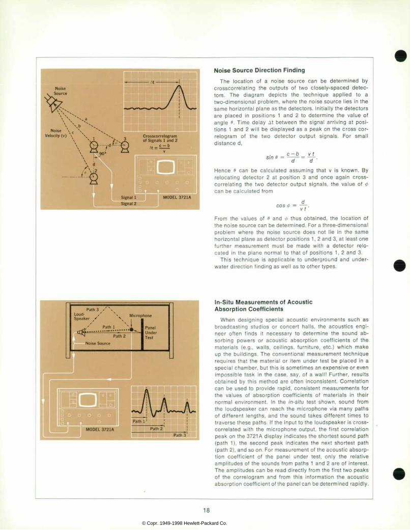
Noise Source Direct ion Finding T h e l o c a t i o n o f a n o i s e s o u r c e c a n b e d e t e r m i n e d b y

c r o s s c o r r e l a t i n g t h e o u t p u t s o f t w o c l o s e l y - s p a c e d d e t e c t o r s . T h e d i a g r a m d e p i c t s t h e t e c h n i q u e a p p l i e d t o a two -d imens iona l p rob lem, whe re t he no i se sou rce l i e s i n t he same hor izon ta l p lane as the de tec to rs . In i t i a l l y the de tec to rs a r e p l a c e d i n p o s i t i o n s 1 a n d 2 t o d e t e r m i n e t h e v a l u e o f a n g l e 9 . T i m e d e l a y A t b e t w e e n t h e s i g n a l a r r i v i n g a t p o s i t i o n s 1 a n d 2 w i l l b e d i s p l a y e d a s a p e a k o n t h e c r o s s c o r - r e l o g r a m o f t h e t w o d e t e c t o r o u t p u t s i g n a l s . F o r s m a l l d i s tance d ,

sin e = c - b v t d

H e n c e e c a n b e c a l c u l a t e d a s s u m i n g t h a t v i s k n o w n . B y r e l o c a t i n g d e t e c t o r 2 a t p o s i t i o n 3 a n d o n c e a g a i n c r o s s - c o r r e l a t i n g t h e t w o d e t e c t o r o u t p u t s i g n a l s , t h e v a l u e o f < / > can be ca l cu la ted f r om

cos <t> = d v t

F r o m t h e v a l u e s o f o a n d < P t h u s o b t a i n e d , t h e l o c a t i o n o f t he no ise source can be de te rm ined . Fo r a th ree -d imens iona l p r o b l e m w h e r e t h e n o i s e s o u r c e d o e s n o t l i e i n t h e s a m e hor izonta l p lane as de tec tor pos i t ions 1 , 2 and 3 , a t leas t one f u r t h e r m e a s u r e m e n t m u s t b e m a d e w i t h a d e t e c t o r r e l o c a t e d i n t h e p l a n e n o r m a l t o t h a t o f p o s i t i o n s 1 , 2 a n d 3 .

T h i s t e c h n i q u e i s a p p l i c a b l e t o u n d e r g r o u n d a n d u n d e r wa te r d i rec t ion f i nd ing as we l l as to o the r t ypes .

In-Situ Measurements of Acoustic Absorption Coeff icients

W h e n d e s i g n i n g s p e c i a l a c o u s t i c e n v i r o n m e n t s s u c h a s b r o a d c a s t i n g s t u d i o s o r c o n c e r t h a l l s , t h e a c o u s t i c s e n g i n e e r o f t e n f i n d s i t n e c e s s a r y t o d e t e r m i n e t h e s o u n d a b s o r b i n g p o w e r s o r a c o u s t i c a b s o r p t i o n c o e f f i c i e n t s o f t h e m a t e r i a l s ( e . g . , w a l l s , c e i l i n g s , f u r n i t u r e , e t c . ) w h i c h m a k e u p t h e b u i l d i n g s . T h e c o n v e n t i o n a l m e a s u r e m e n t t e c h n i q u e r e q u i r e s t h a t t h e m a t e r i a l o r i t e m u n d e r t e s t b e p l a c e d i n a spec ia l chamber , bu t t h i s i s somet imes an expens ive o r even i m p o s s i b l e t a s k i n t h e c a s e , s a y , o f a w a l l ! F u r t h e r , r e s u l t s o b t a i n e d b y t h i s m e t h o d a r e o f t e n i n c o n s i s t e n t . C o r r e l a t i o n c a n b e u s e d t o p r o v i d e r a p i d , c o n s i s t e n t m e a s u r e m e n t s f o r t h e v a l u e s o f a b s o r p t i o n c o e f f i c i e n t s o f m a t e r i a l s i n t h e i r n o r m a l e n v i r o n m e n t . I n t h e i n - s i t u t e s t s h o w n , s o u n d f r o m t h e l o u d s p e a k e r c a n r e a c h t h e m i c r o p h o n e v i a m a n y p a t h s o f d i f f e r e n t l e n g t h s , a n d t h e s o u n d t a k e s d i f f e r e n t t i m e s t o t raverse these pa ths . I f the inpu t to the loudspeaker i s c ross - c o r r e l a t e d w i t h t h e m i c r o p h o n e o u t p u t , t h e f i r s t c o r r e l a t i o n peak on the 3721A d i sp lay i nd i ca tes the sho r tes t sound pa th ( p a t h 1 ) , t h e s e c o n d p e a k i n d i c a t e s t h e n e x t s h o r t e s t p a t h (pa th 2 ) , and so on . Fo r measuremen t o f t he acous t i c abso rp t i o n c o e f f i c i e n t o f t h e p a n e l u n d e r t e s t , o n l y t h e r e l a t i v e amp l i t udes o f t he sounds f r om pa ths 1 and 2 a re o f i n t e res t . The amp l i t udes can be read d i r ec t l y f r om the f i r s t two peaks o f t h e c o r r e l o g r a m a n d f r o m t h i s i n f o r m a t i o n t h e a c o u s t i c absorp t ion coe f f i c ien t o f the pane l can be de te rmined rap id ly .


C r o s s c o r r e l a t i o n o f E l e c t r o m y o g r a m s

T h e e l e c t r o m y o g r a m ( E M G ) Â ¡ s a r e c o r d o f m u s c u l a r e l e c t r i c a l a c t i v i t y , w h i c h c a n a s s i s t i n t h e d i a g n o s i s o f n e r v o u s a n d m u s c u l a r d i s e a s e s . W h e n d e t e c t e d b y a n e e d l e e l e c t r o d e , t h e E M G c o n s i s t s o f a s e r i e s o f p u l s e s r e p r e s e n t i n g the e lec t r i ca l ac t i v i t y o f the musc le ce l l s i n the v i c in i t y o f the e l e c t r o d e . A u s e f u l m e a s u r e o f f a t i g u e o r d i s e a s e i n a m u s c l e i s t h e e x t e n t t o w h i c h t h e c e l l s f i r e i n d e p e n d e n t l y o f e a c h o t h e r . T h e c r o s s c o r r e l o g r a m o f t h e t w o E M G ' s f r o m a m u s c l e w i l l s h o w w h e t h e r t h e c e l l s a r e t e n d i n g t o f i r e t o g e t h e r o r r a n d o m l y . T h e d i a g r a m c o n t r a s t s t h e c r o s s c o r r e l o g r a m o b t a i n e d f r o m a h e a l t h y s u b j e c t w i t h t h a t a c q u i r e d f r o m a p a t i e n t s u f f e r i n g f r o m t h e a f t e r e f f e c t s o f po l i omye l i t i s . W i th the hea l thy sub jec t , t he c rossco r re log ram o f s i g n a l s 1 a n d 2 s h o w s i n d e p e n d e n t f i r i n g o f t h e c e l l s w h e n t h e m u s c l e i s r e l a x e d , w i t h c o r r e l a t i o n i n c r e a s i n g a s t he musc le con t rac t s on l oad . Whe re t he pa t i en t i s su f f e r i ng f r o m i s a f t e r e f f e c t s o f p o l i o m y e l i t i s , t h i s c o r r e l a t i o n i s p r o m i n e n t e v e n i n t h e r e l a x e d s t a t e o f t h e m u s c l e , a n d i t i n c r e a s e s r a p i d l y o n l o a d a s t h e m u s c l e b e c o m e s t i r e d . T h e c r o s s c o r r e l o g r a m d i s p l a y e d b y t h e M o d e l 3 7 2 1 A i s , t h e r e fo re , a use fu l gu ide to musc le cond i t ion .

Measurement of Torsion in Rotat ing Shafts

C o r r e l a t i o n t e c h n i q u e s c a n b e u s e d t o m e a s u r e t o r s i o n i n a p o w e r t r a n s m i s s i o n s h a f t u n d e r o p e r a t i n g c o n d i t i o n s , b y a c c u r a t e l y d e t e c t i n g a c h a n g e i n p h a s e a n g l e b e t w e e n t he ou tpu t s i gna l s o f t r ansduce rs p l aced a t e i t he r end o f t he s h a f t . I n t h e e x a m p l e i l l u s t r a t e d , t h e t w i s t i n a l o n g t r a n s m i s s i o n s h a f t i s b e i n g m e a s u r e d . M a g n e t i c p i c k u p s a r e p l a c e d a d j a c e n t t o t h e u n i v e r s a l j o i n t s a t t h e e n d s o f t h e sha f t so t ha t when t he sha f t r o t a tes each p i ckup p roduces a t r a i n o f r e g u l a r p u l s e s w i t h p e r i o d p r o p o r t i o n a l t o t h e s h a f t s p e e d . C r o s s c o r r e l a t i o n o f t h e p i c k u p o u t p u t s i g n a l s y i e l d s a c o r r e l o g r a m w h o s e p e a k s a r e s p a c e d T ( s e c o n d s ) a p a r t , T be ing the pu lse repe t i t i on pe r iod . I f a l oad ( to rque) change o c c u r s , t h e p h a s e a n g l e b e t w e e n t h e o u t p u t s i g n a l s o f t h e p i c k u p s w i l l c h a n g e r e s u l t i n g i n a n o v e r a l l m o v e m e n t r o f t h e d i s p l a y e d p e a k s . T h i s c h a n g e T w i l l g i v e a m e a s u r e o f t h e s h a f t t w i s t a n d h e n c e o f t h e t o r q u e i t i s t r a n s m i t t i n g . Th is techn ique can be app l i ed to any s i t ua t i on i n wh ich l a rge powers a re be ing t r ansm i t t ed a long ro ta t i ng sha f t s .

Contact less Veloci ty Measurement Measu remen t o f t he ve l oc i t y o f s t ee l s t r i p o r shee t f r om a

r o l l i n g m i l l i s a d i f f i c u l t p r o b l e m w h e n t h e m e t a l i s c o l d , b u t w h e n t h e m e t a l i s w h i t e h o t , t h e d i f f i c u l t y i s i n c r e a s e d g rea t l y . Con tac t less measurement o f the ve loc i t y i s poss ib le , howeve r , us i ng a C rossco r re l a t i on t echn ique . The t echn ique i s i l l us t ra ted in the d iagram. When meta l i s ro l led , i t s sur face i s n o t t h e s m o o t h a n d a n y i r r e g u l a r i t i e s w i l l a f f e c t t h e o u t p u t o f a p h o t o c e l l w h i c h i s f o c u s e d o n t h e s u r f a c e . A f t e r a f i n i t e t ime , each i r regu la r i t y w i l l pass the focus ing po in t o f a s e c o n d s i m i l a r p h o t o c e l l p l a c e d d o w n s t r e a m f r o m t h e f i r s t o n e . C r o s s c o r r e l a t i o n o f t h e t w o p h o t o c e l l o u t p u t s i g n a l s u s i n g t h e 3 7 2 1 A C o r r e l a t o r w i l l i n d i c a t e t h e t i m e d e l a y T d d i r e c t l y . I f t h e p h o t o c e l l s e p a r a t i o n d i s k n o w n , t h e v e l o c i t y v o f t h e s t r i p o r s h e e t l e a v i n g t h e r o l l e r s c a n b e d e t e r m i n e d s i m p l y f r o m :

d v = T -


(e)

(o)

Speech Research A m o n g m a n y t o p i c s o f c u r r e n t i n t e r e s t i n t h e a u d i o f i e l d

w h i c h d e m a n d m o r e p r e c i s e b a s i c k n o w l e d g e o f h u m a n s p e e c h a r e t h e r e d u c t i o n o f s p e e c h b a n d w i d t h f o r t e l e c o m m u n i c a t i o n p u r p o s e s , t h e e d u c a t i o n o f t h e d e a f , a n d t h e p r o v i s i o n o f m a n - c o m p u t e r i n t e r f a c e s w h i c h s p e a k h u m a n l a n g u a g e s r a t h e r t h a n m a c h i n e l a n g u a g e s . A l t h o u g h s p e c t r a l a n a l y s i s i s a w e l l - e s t a b l i s h e d t o o l f o r c h a r a c t e r i z i n g a u d i o s i g n a l s , c o r r e l a t i o n t e c h n i q u e s , w h i c h p r e s e n t t h e s a m e i n f o r m a t i o n i n t h e t i m e d o m a i n , a r e o f t e n m o r e u s e f u l w h e r e s p e e c h i s c o n c e r n e d . U s i n g t h e 3 7 2 1 A C o r r e l a t o r , t he au toco r re l a t i on o f speech s i gna l s can be pe r f o rmed ve ry s i m p l y . T h e t w o p h o t o g r a p h s s h o w t h e a u t o c o r r e l a t i o n f u n c t i o n s o f t w o c o m m o n s p e e c h s o u n d s : ' e ' a s i n ' t r e e , ' a n d ' o ' a s i n ' m o l e . ' T h e s e f u n c t i o n s w e r e o b t a i n e d w i t h i n s e c o n d s f r o m d i r e c t s p e e c h i n t o a m i c r o p h o n e c o n n e c t e d t o t h e Mode l 3721A.

Radio Astronomy The de tec t i on o f ve ry weak and ve ry d i s tan t r ad io sou rces

i n space i s ca r r i ed ou t by h i gh -ga in r ad io t e l escopes . These t e l e s c o p e s a r e e x t r e m e l y s e n s i t i v e t o i n t e r f e r e n c e f r o m r a n d o m e l e c t r i c a l d i s t u r b a n c e s , w h i c h t e n d t o m a s k t h e s m a l l s i gna ls o f i n te res t . However , i n some cases â€ ” e .g . , pu l sa rs â € ” t h e s i g n a l s o f i n t e r e s t a r e p e r i o d i c , a n d b y u s i n g t h e M o d e l 3 7 2 1 A a n d a u t o c o r r e l a t i o n t e c h n i q u e s , t h e p e r i o d i c c o m p o n e n t o f t h e r e c e i v e d s i g n a l c a n b e e x t r a c t e d f r o m t h e n o i s e . T h e m e t h o d i s b a s e d o n t h e p r i n c i p l e t h a t , a f t e r a n a p p r e c i a b l e d e l a y , t h e a u t o c o r r e l a t i o n f u n c t i o n o f t h e n o i s e c o m p o n e n t w i l l h a v e d i e d a w a y t o z e r o , b u t t h e p e r i o d i c c o m p o n e n t w i l l h a v e a p e r i o d i c a u t o c o r r e l a t i o n f u n c t i o n wh i ch w i l l pe r s i s t a t a l l de l ays . A s imp le de tec t i on sys tem i s i l l u s t r a t e d i n t h e d i a g r a m . T h e r e a r e n o t h e o r e t i c a l l i m i t s t o t h e a u t o c o r r e l a t i o n m e t h o d . A n y p e r i o d i c s i g n a l c a n b e d e t e c t e d i n t h e p r e s e n c e o f n o i s e . B e s i d e s r a d i o a s t r o n o m y , t h i s t e c h n i q u e c a n b e u s e d i n m a n y o t h e r b r a n c h e s o f r e search â€” medica l , acoust ica l , v ib ra t ion and communicat ions.

Determination of Noise Transmission Paths U n w a n t e d n o i s e a n d v i b r a t i o n s o f t e n t r a v e l t o t h e e a r o f

t h e h e a r e r v i a s e v e r a l d i f f e r e n t p a t h s . I f t h e s e p a t h s c a n b e d e t e r m i n e d , s t e p s c a n b e t a k e n t o m i n i m i z e o r e l i m i n a t e the i r e f fec ts . Cor re la t ion techn iques can be used to de termine n o i s e t r a n s m i s s i o n p a t h s . F o r e x a m p l e , i n t h e a u t o m o b i l e i n d u s t r y i t m a y b e d e s i r a b l e t o d e t e r m i n e t h e n o i s e t r a n s m i ss i on pa ths f r om the f r on t ax l e o f a ca r t o t he d r i ve r . Th i s c a n b e d o n e b y p l a c i n g a t r a n s d u c e r o n t h e a x l e a n d a m i c r o p h o n e i n s i d e t h e c a r i n t h e v i c i n i t y o f t h e d r i v e r ' s h e a d , a n d c r o s s c o r r e l a t i n g t h e o u t p u t s o f t h e t r a n s d u c e r a n d t h e m i c r o p h o n e . I n t h e e x a m p l e i l l u s t r a t e d , t h e n o i s e f r om the f r on t ax l e i s t r ansm i t t ed p r ima r i l y t h rough t he s tee r i ng co l umn (pa th 1 ) and v i a t he f l oo r and d r i ve r ' s sea t ( pa th 2 ) . T h e c o r r e l o g r a m d i s p l a y s t w o p e a k s w i t h t i m e d e l a y s r e p r e s e n t a t i v e o f t h e i n d i v i d u a l t r a n s m i s s i o n p a t h d e l a y s . E x a m i n a t i o n o f t h e a m p l i t u d e o f t h e p e a k s w i l l g i v e a m e a s ure o f the re la t i ve amounts o f no ise t ransmi t ted by each path .

HEWLETT-PACKARD JOURNAL <z>" NOVEMBER 1969 volume 21 -Numbers T E C H N I C A L C A L I F O R N I A F R O M T H E L A B O R A T O R I E S O F T H E H E W L E T T - P A C K A R D C O M P A N Y P U B L I S H E D A T 1 5 0 1 P A G E M I L L R O A D , P A L O A L T O , C A L I F O R N I A 9 4 3 0 4

Editor: Assistant: H Jordan Editorial Board: R. P. Dolan. L. D. Shergalis Art Director: Arvid A. Danielson Assistant: Maride! Jordan


hp journal 1969 - correlation

Documents