how well do energy efﬁciency measures actually perform? · the standard assessment procedure...

How well do energy efficiencymeasures actually perform?Daire McCoy (LSE, ESRI), Raphaela Kotsch (LSE)Grantham Research Institute, LSE

Policies to Finance Energy Efficiency, LSE. 1st June 2018

Introduction

Introduction and motivation

Expections vs

�There is no realistic, or a�ordable, energy development strategy that

is not led by energy e�ciency. For the IEA, it is the �rst fuel" - FatihBirol, 2016

Reality?

2 / 30

Introduction


Fowlie at al. (2015), Allcott and Greenstone (2017)

• Actual energy savings 40-60 percent of predicted

Gerarden at al. (2015) energy e�ciency gap

• Market failures, behavioural failures, model/measurement error

• Unobserved costs, overstated savings from adoption, consumerheterogeneity, inappropriate discount rates and uncertainty contributeto low adoption rate not being as �paradoxical as it �rst appears.�

Kotchen (2017) long-run e�ects of building regulations

• E�ects of code change on electricity consumption diminish over time

• E�ects on gas consumption increase over time

3 / 30

Introduction


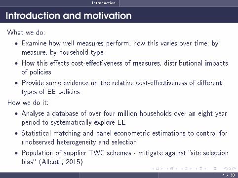
What we do:

• Examine how well measures perform, how this varies over time, bymeasure, by household type

• How this e�ects cost-e�ectiveness of measures, distributional impactsof policies

• Provide some evidence on the relative cost-e�ectiveness of di�erenttypes of EE policies

How we do it:

• Analyse a database of over four million households over an eight yearperiod to systematically explore EE

• Statistical matching and panel econometric estimations to control forunobserved heterogeneity and selection

• Population of supplier TWC schemes - mitigate against �site selectionbias" (Allcott, 2015)

4 / 30

Introduction

Presentation overview

• Background

• Data

• Methods

• Results

5 / 30

Background

Background

• UK Supplier Obligations (Tradeable White Certi�cates)• Principal policy instrument in UK• Also widely used in Europe (Italy, France)• Hybrid subsidy-tax instrument (Giraudet, 2012)

• Three main features (Bertoldi and Rezessy, 2008):1 An obligation is placed on energy companies to achieve a quanti�ed

target of energy savings2 Savings are based on standardised ex-ante calculations3 The obligations can be traded with other obligated parties

• Market-based �exibility aims to encourage cost-e�ectiveness

• Suppliers bear the cost and then pass through to their customers

• Widely considered to have been a cost e�ective measure

6 / 30

Background

Background

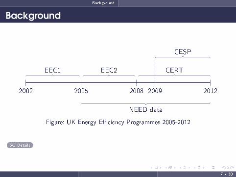
2002 2005 2008 2009 2012

EEC1 EEC2 CERT

CESP

NEED data

Figure: UK Energy E�ciency Programmes 2005-2012

SO Details

7 / 30

Background

Background

Table: Energy savings by scheme and measure

EEC1 EEC2 CERT2002-2005 2005-2008 2008-2012

Insulation 56% 75% 66.20%Heating 9% 8% 8.20%Lighting 24% 12% 17.30%Appliances 11% 5% 5.90%Other - - 2.40%Source: Lees (2005, 2008), Ofgem (2013)

8 / 30

Data

NEED database

National Energy E�ciency Data-Framework (NEED)

Table: Data sources combined in NEED

Type of variable SourceEnergy e�ciency measures HEED/Ofgem/DECCEnergy consumption Energy SuppliersProperty attributes VOAHousehold characteristics ExperianSource: DECC/BEIS

IMD

9 / 30

Data

Measures installed

Measures installed

01

00

00

02

00

00

03

00

00

04

00

00

05

00

00

0N

um

be

r o

f u

pg

rad

es

2005 2006 2007 2008 2009 2010 2011 2012year

Cavity wall insulation Loft insulationReplacement boiler All

Figure: Energy e�ciency measuresinstalled, 2005-2012

Energy consumption

05

00

01

00

00

15

00

02

00

00

Ave

rag

e c

on

su

mp

tio

n (

kW

h)

2005 2006 2007 2008 2009 2010 2011 2012Year

Gas Electricity

Figure: Average domestic energyconsumption (kWh) UK, 2005-2012

10 / 30

Analysis

Non-random assignment

• Households are not randomly assigned measures. They chose to availof supplier o�ers

• Selection into scheme is likely correlated with energy consumption,income, location and other factors...

• Not taking this into account would bias results

• Pre-process data using coarsened-exact matching to reduce imbalancein observed variables (Iacus, King, and Porro, 2008; Alberini andTowe, 2015)

• Match on variables most likely to (i)predict selection into scheme, (ii)energy consumption (iii) level and trend of prior year's energyconsumption

11 / 30

Analysis

Identification: Matching

Figure: Assignment to treatment and control

12 / 30

Analysis

Matching results: energy consumption

0.0

001

.000

2kd

ensi

ty E

cons

2005

0 5000 10000 15000 20000 25000Electricity consumption 2005 (kWh)

Control Upgrade

Before matching

0.0

001

.000

2

0 5000 10000 15000 20000 25000Electricity consumption 2005 (kWh)

Control Upgrade

After matching0

.000

02.0

0004

.000

06kd

ensi

ty G

cons

2005

0 10000 20000 30000 40000Gas consumption 2005 (kWh)

Control Upgrade

0.0

0002

.000

04.0

0006

0 10000 20000 30000 40000Gas consumption 2005 (kWh)

Control Upgrade

Figure: Energy consumption before and after matching

Balance tables13 / 30

Analysis

Matching results: parallel paths

Upg

rade

per

iod

1200

014

000

1600

018

000

2004 2006 2008 2010 2012year

Upgrade Control

1200

014

000

1600

018

000

2004 2006 2008 2010 2012year

Upgrade Control

1200

014

000

1600

018

000

2000

0

2004 2006 2008 2010 2012year

Upgrade Control

1200

014

000

1600

018

000

2000

0

2004 2006 2008 2010 2012year

Upgrade Control

1200

014

000

1600

018

000

2004 2006 2008 2010 2012year

Upgrade Control

1200

014

000

1600

018

000

2000

0

2004 2006 2008 2010 2012year

Upgrade Control

Figure: Consumption trend: Treatment and control group

Balance tables14 / 30

Analysis

Econometric approach

First-di�erenced �xed-e�ects panel estimation:

ln(yit) = αi + γt + ρrt + δ

J∑j=1

Dijt + εit (1)

Where:

• yit - energy consumption by household i in year t

• αi - household �xed e�ect

• γt - year dummy

• ρrt - year*region interaction

• Dit - treatment dummy

• δ - ATT

• εit - error term

15 / 30

Results

Results overview

• R1: Main results

• R2: Heterogeneity in returns

• R3: Comparison with ex-ante predictions

• R4: Cost e�ectiveness

16 / 30

Results

R1: Main results

Table: The e�ect of energy e�ciency upgrades on energy consumption

(1) (2) (3) (4) (5) (6) (7)Full sample 2006 upgrades 2007 upgrades 2008 upgrades 2009 upgrades 2010 upgrades 2011 upgrades

Cavity wall insulation -0.094*** -0.097*** -0.111*** -0.099*** -0.098*** -0.097*** -0.101***(0.001) (0.002) (0.003) (0.002) (0.002) (0.002) (0.002)

Loft insulation -0.030*** -0.026*** -0.031*** -0.028*** -0.027*** -0.039*** -0.035***(0.001) (0.003) (0.003) (0.002) (0.002) (0.002) (0.002)

Replacement boiler -0.092*** -0.080*** -0.093*** -0.087*** -0.102*** -0.109*** -0.099***(0.001) (0.002) (0.002) (0.002) (0.002) (0.002) (0.002)

Control variables Y Y Y Y Y Y YHousehold �xed e�ects Y Y Y Y Y Y YYear �xed e�ects Y Y Y Y Y Y YYear*region �xed e�ects Y Y Y Y Y Y Y

Observations 5502936 617022 545627 564756 730447 746573 871379Number of households 687925 77128 68203 70595 91306 93322 108922R squared 0.349 0.327 0.353 0.370 0.369 0.386 0.367

Notes: This table reports coe�cient estimates and standard errors from eight separate regressions. The dependentvariable in all regressions is the logarithm of annual gas consumption in kilowatt hours. Column(1) "All" denotese�ciency upgrades occurring at any time during the sample period. Columns (2-8) relate to upgrades occurring onlyin the relevant year. Each individual year denotes upgrades occurring solely in that year. For each upgrade group amatched control group is created using coarsened-exact matching. The sample includes billing records from 2005 to2012. Standard errors are clustered at the household level. Triple asterisks denote statistical signi�cance at the 1%level; double asterisks at the 1% level; single asterisks at the 10% level.

17 / 30

Results

R2: Heterogeneity in returns

−.1

1−

.1−

.09

−.0

8−

.07

−.0

6A

TT

1 2 3 4 5IMD group

Cavity wall insulation

−.0

45−

.04−

.035

−.0

3−.0

25−

.02

1 2 3 4 5IMD group

Loft insulation−

.1−

.09

−.0

8−

.07

−.0

6A

TT

1 2 3 4 5IMD group

Replacement heating system

Figure: ATT by IMD group, all periods18 / 30

Results


Upg

rade

per

iod

−.1

2−

.1−

.08−

.06−

.04−

.02

0A

TT

2005 2006 2007 2008 2009 2010 2011 2012year

Loft insulation over time

−.1

2−.1

−.0

8−.0

6−.0

4−.0

20

2005 2006 2007 2008 2009 2010 2011 2012year

Cavity wall insulation over time−

.12

−.1

−.0

8−.0

6−.0

4−.0

20

AT

T

2005 2006 2007 2008 2009 2010 2011 2012year

Boiler upgrades over time

Figure: ATT over time for measure installed in 200619 / 30

Results


Upg

rade

per

iod

−.1

2−

.1−

.08

−.0

6−

.04

−.0

20

AT

T

20052006200720082009201020112012year

All groups

−.1

2−

.1−

.08

−.0

6−

.04

−.0

20

2005 2006 2007 2008 2009 2010 2011 2012year

IMD1

−.1

2−

.1−

.08

−.0

6−

.04

−.0

20

2005 2006 2007 2008 2009 2010 2011 2012year

IMD2−

.12

−.1

−.0

8−

.06

−.0

4−

.02

0A

TT

20052006200720082009201020112012year

IMD3−

.12

−.1

−.0

8−

.06

−.0

4−

.02

0

2005 2006 2007 2008 2009 2010 2011 2012year

IMD4

−.1

2−

.1−

.08

−.0

6−

.04

−.0

20

2005 2006 2007 2008 2009 2010 2011 2012year

IMD5

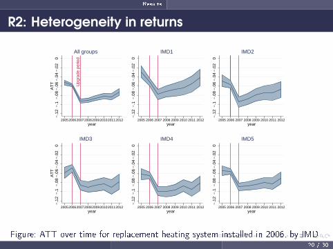
Figure: ATT over time for replacement heating system installed in 2006, by IMDgroup 20 / 30

Results

R3: Comparison with ex-ante SAP predictions

• The Standard AssessmentProcedure (SAP)

• Bottom-up engineering modeldeveloped by BRE

Measuresinstalled

SAP predicted(kWh)

Empirical esti-mates (kWh)

Percentage of

predicted

Cavity wall in-sulation

2724 1278 47%

Loft insulation 671 384 57%Replacementheating system

3588 1328 37%

Source of SAP predicted savings: Adapted from Dowson (2012) Shorrock (2005)

21 / 30

Results

Results summary

• Cavity wall insulation and replacement heating systems - approx 9%.Loft insulation - approx 3%

• Savings are greater for less deprived households

• Savings are more stable over time for less deprived households

• Bottom-up engineering model overstate savings by 43-63%

• What does this mean in terms of cost-e�ectiveness?

• As measured by IRR, cost per kWh o� energy saved, cost per tonne ofCO2 removed

22 / 30

Results

Some assumptions requiredAbout (i) energy prices

0.00000

0.02000

0.04000

0.06000

0.08000

0.10000

0.12000

0.14000

1996 2006 2016 2026

£/k

Wh

Year

BEIS high gas

price forecast

BEIS low gas

price forecast

Actual Projected

Figure: Gas prices ±5%

(ii) estimated cost of measures

Table: Cost estimates

Measure Cost assumptions (¿)

Cavity wall insulation 350Loft insulation 285Replacement boiler (policy cost) 200Replacement boiler (private cost) 2000

Source: Authors calculations based on Lees (2005, 2008)

Shorrock (2005) EST (2013)

(iii) estimated lifespan of measures...

23 / 30

Results

Internal Rate of Return (IRR)

Table: IRR of measures

IRR 10 IRR 20 IRR 30

Cavity wall insulation 3% 12% 13%Loft insulation -13% 0% 3%Replacement heating (200) 17% 22% 23%Replacement heating (2000) -22% -6% -1%

24 / 30

Results

Cost effectiveness

Table: Cost per tonne of CO2 removed and per kWh of energy saved

¿ per tonne of CO2 ¿ per kWh

Cavity wall insulation 36 0.0072Loft insulation 90 0.0171Replacement heating (200) 60 0.0141Replacement heating (2000) 600 0.1412

Note: Calculated using Carbon Trust estimates

of CO2 per kWh of electricity and gas

25 / 30

Results

Cost effectiveness

Table: How does this compare?

Intervention type Reference Evaluation type Relevant subset Percent reduc-tion in energyusage

Engineering es-timates of per-cent reductionin energy usage

Cost e�ective-ness (cents perkWh saved,2015 USD)

Behavioral programs Allcott (2011) RCT NA 2 3.6Allcott & Rogers (2014) RCT One-shot intervention 4.4

Two-year intervention 1.1 to 1.8Four-year intervention 1.2 to 1.8

Ayres et al. (2012) RCT Sacramento, California 2 5.5Puget Sound, Washington 1.2 2

Building codes Novan et al. (2017) RD analysis NA 1.3 20 24.4

E�cient equipment or energysavings subsidy

Alberini & Towe (2015) Matching NA 5.3 3.9

Alberini et al. (2016) DID Rebate of $1,000 or more 0Rebate of $450 5.5 47.9Rebate of $300 6.2 28.2

Burlig et al. (2017) Machine learning NA 2.9 to 4.5 11.6 to 18Davis et al. (2014) DID regression Refrigerators 8 27.2

Air conditioners plus 1.7 4.5

Information provision Alberini & Towe (2015) Matching 5.5

UK Supplier Obligation (TWC) McCoy & Kotsch (2018) Matching, FE regression Cavity wall insulation 9.4 20.0 1.54 to 2.31Loft insulation 3 5.2 3.65 to 5.47Replacement heating system 9.2 24.9 3.02 to 30.19

Previous estimate 1.92

Adapted from Gillingham et al(2018)

26 / 30

Conclusions

ConclusionsKey �ndings:

• Measures funded by UK Supplier Obligations delivered signi�cantsavings for households

• Considerable variation by measure, household type and over time

• Considerably less than engineering model estimates

• Despite this they were cost-e�ective and compare favourable withother schemes

• Distributional concerns despite explicit targets for deprived households

Policy implications:

• Underlines need to use actual rather than estimated savings

• Evaluations need to better quantify non-�nancial savings. Particularlycomfort and health bene�ts of EE

• Variation in returns has implications for policy prescription: Lowinterest loans may need to be very low interest for some households

27 / 30

Summary of EIBURS project


Key �ndings:

• WP 1: Characterised and presented an overview of the key informationasymmetries which e�ect adoption of energy e�ciency measures

• WP 2: Provides an empirical analysis of whether banks are pricingenergy e�ciency projects e�ciently. Evidence suggests they are not

• WP 3.1: Outlines the key empirical challenges in performing robustenergy e�ciency project evaluations

• WP 3.2: Examines how well energy e�ciency measures actuallyperform. UK measures have been largely cost e�ective, but need tobetter quantify all costs and bene�ts, and some distributionalconcerns.

• Next steps: Finalise results, submit report to EIB and submit papersto peer-review journals.

28 / 30



Where to go next:

• Help banks to price EE projects e�ciently. Mobilise �nance through�Green Tagging� and better quanti�cation the associated risks of�green" vs other portfolios

• �Energy Epidemiology� - leverage more data, smart meters,randomised-controlled trials to better measure energy performance

29 / 30

End

[email protected]

30 / 30

Overview of Supplier Obligations

Table: Overview of Supplier Obligations

ECC1 ECC2 CERT CESPTarget 62 TWh 130 TWh 293 million t CO2

=494TWh19.25 MtCO2

Costs 167 mil-lion

400 mil-lion

1,158 million unknown

% savings in prioritygroup

50% 50% 40% lowest 10-15% ofareas rankedby IMD

# cavity wall insulations 791,524 1,336,374 2,568,870 3,000# loft insulations 528,496

(lofttop up,15,979,367DIY inm2)

1,980,445 3,897,324 (professional),112,850,996 (DIY in m2)

23,503

# replacement boilers 195,832(Hotwatertank)

2,082,812 31,986 42,898

Source: Lees 2005, 2008; Rosenow, 2012; Ofgem, 2013

Background

IMD

Table: Composition of IMD in %

England 2010 Wales 2011Income 22.5 23.5Employment 22.5 23.5Health 13.5 14Education 13.5 14Access/barriers to services 9.3 10Living environment/ housing 9.3 5Physical environment 0 5Crime [Wales: Community Safety] 9.3 5

NEED Overview

Matching

• FE estimator assumes Dit is strictly exogenous and randomly assigned

• Its likely that selection into upgrade is correlated with energyconsumption

• Leading to biased estimates

• Pre-process data using CEM to reduce imbalance in observed variables(Iacus, King, and Porro, 2008; Alberini and Towe, 2015)

• Match on variables most likely to predict (i)selection into scheme, (ii)energy consumption; prior year's energy consumption

• Excellent balance on matched, needs improvement on unmatched

• Currently comparing CEM with Nearest Neighbour, Kernel andMahalanobis metric matching

Matching results

Table: Percentage matched

Dwellings receiving upgrades Count

Full database 1,869,3722005 or unknown upgrade date 416,994Remaining sample 1,452,378Matched sample 1,286,419Unmatched 165,959Matched as a percentage of eligible 89%

Standardised di�erence:

d =xtreatment − xcontrol√

s2treatment+s2control2

(2)

Variance ratio:

F =s2treatment

s2control(3)

Elec/gas matched

Matching results

Table: Balance table for full database

Unmatched sample Treated Control Balance

Variable Mean Variance Skewness Mean Variance Skewness Std-di� Var-ratio

prop_age 2.96 1.98 0.16 3.00 3.00 0.31 -0.03 0.66imd_both 2.85 2.11 0.15 2.96 2.01 0.05 -0.08 1.05region 5.34 7.33 0.03 5.81 6.31 -0.29 -0.18 1.16fuel_type 0.98 0.02 -7.43 0.98 0.02 -6.33 0.04 0.74Gcons2005 18124 78900000 0.65 17394 86200000 0.73 0.08 0.92

prop_type 3.33 2.63 0.22 3.56 2.92 0.08 -0.14 0.90�oor_area 2.20 0.40 0.89 2.20 0.46 0.77 -0.01 0.86loft_depth 2.03 0.28 0.04 2.08 0.53 -0.13 -0.08 0.52wall_cons 0.73 0.20 -1.02 0.59 0.24 -0.36 0.29 0.82FP_ENG 2.95 1.97 0.06 2.89 2.12 0.10 0.04 0.93Econs2005 3903 7653561.00 2.16 3998.54 8374713 2.14 -0.03 0.91

Elec/gas matched

Matching results

Table: Balance table for full matched sample

All years matched Treated Control Balance


prop_age 2.91 2.32 0.24 2.91 2.31 0.24 0.00 1.00imd_both 2.92 2.07 0.09 2.92 2.07 0.09 0.00 1.00region 5.62 6.83 -0.15 5.62 6.82 -0.15 0.00 1.00fuel_type 0.98 0.02 -7.45 0.98 0.02 -7.47 0.00 1.01

Gcons2005 18020 84200000 0.67 18017 84300000 0.67 0.00 1.00prop_type 3.36 2.68 0.19 3.48 2.87 0.14 -0.07 0.93�oor_area 2.21 0.42 0.86 2.21 0.45 0.80 0.00 0.93loft_depth 2.04 0.30 0.03 2.05 0.52 -0.08 -0.02 0.57wall_cons 0.67 0.22 -0.71 0.63 0.23 -0.52 0.09 0.95FP_ENG 2.95 2.04 0.06 2.96 2.09 0.05 -0.01 0.98Econs2005 3945.89 7999389.00 2.15 4028.94 8182317.00 2.09 -0.03 0.98

Elec/gas matched

Matching results

Table: Balance table for 2006 matched sample

2006 Matched Treated Control Balance


prop_age 2.90 2.02 0.19 2.93 2.09 0.21 -0.02 0.97imd_both 2.79 2.07 0.20 2.80 2.07 0.19 -0.01 1.00region 5.42 7.24 -0.03 5.43 7.22 -0.03 0.00 1.00fuel_type 0.99 0.01 -9.10 0.99 0.01 -9.14 0.00 1.01Gcons2005 17844 82300000 0.61 17829 81900000 0.61 0.00 1.00

prop_type 3.49 2.78 0.14 3.52 2.87 0.13 -0.02 0.97�oor_area 2.17 0.43 0.81 2.18 0.43 0.79 -0.02 0.98loft_depth 2.05 0.36 -0.02 2.06 0.51 -0.08 0.00 0.71wall_cons 0.69 0.21 -0.81 0.65 0.23 -0.62 0.08 0.94FP_ENG 2.95 2.01 0.05 2.96 2.06 0.05 0.00 0.97Econs2005 3915.91 8361364.00 2.17 3957.42 7897173.00 2.13 -0.01 1.06

Elec/gas matched

Matching results

Table: Balance table for 2011 matched sample

2011 Matched Treated Control Balance


prop_age 2.97 2.30 0.22 2.97 2.30 0.22 0.00 1.00imd_both 2.94 2.10 0.06 2.94 2.10 0.06 0.00 1.00region 5.55 6.95 -0.11 5.55 6.95 -0.11 0.00 1.00fuel_type 0.98 0.02 -6.92 0.98 0.02 -6.87 0.00 0.99Gcons2010 14490 67800000 0.91 14410 68300000 0.91 0.01 0.99

prop_type 3.29 2.70 0.24 3.46 2.91 0.15 -0.10 0.93�oor_area 2.24 0.43 0.87 2.22 0.46 0.80 0.03 0.94loft_depth 2.03 0.31 0.01 2.06 0.51 -0.08 -0.03 0.61wall_cons 0.67 0.22 -0.74 0.64 0.23 -0.59 0.07 0.95FP_ENG 2.95 2.02 0.06 2.97 2.06 0.04 -0.02 0.98Econs2010 3508.37 6440704.00 2.14 3615.08 6580746.00 2.17 -0.04 0.98

Elec/gas matched

Cost assumptions

Table: Assumptions for costs ofmeasures

Low (¿) High (¿)

Cavity wall (pre 1976) 300 325Cavity wall (post 1976) 300 325Loft 300mm (currently none) 138 273Loft 300mm (currently 100mm) 86 211Loft 300mm (currently 200mm) 35 170Condensing boiler 100 300

Source: Shorrock (2005)

Table: Assumptions for costs ofmeasures

(1994) (2005)

EESOP1 EESOP2 EESOP3 EEC1

Cavity wall insulation 223 219 261 261Condensing boiler 450 270 165 114

Source: Lees (2005)

Cost e�ectiveness

Table: Assumptions for costs of measures

Defra EEC1 Defra EEC2 Defra CERT Lees 2005 Lees 2008

Cavity wall insulation 268 313 380 274 350Loft insulation (top up) 213 260 286 217 275Loft insulation (virgin) 213 260 286 252 295A and B boiler 145 120A and B boiler and heating control 217 190All boilers 50 45

Source: Lees (2005, 2008)

R3: Comparison with ex-ante SAP predictions

Figure: Predicted savings for typical semi-detached dwelling. Source: Shorrock(2005); Dowson (2012)

Results 2

Table: The e�ect of energy e�ciency upgrades on energy consumption for varyinglevels of area-level deprivation in England and Wales

(1) (2) (3) (4) (5) (6)All IMD_BOTH=1 IMD_BOTH=2 IMD_BOTH=3 IMD_BOTH=4 IMD_BOTH=5

(b/se) (b/se) (b/se) (b/se) (b/se) (b/se)Cavity wall insulation -0.083*** -0.063*** -0.078*** -0.090*** -0.092*** -0.098***

(0.001) (0.003) (0.002) (0.002) (0.002) (0.002)Loft insulation -0.018*** 0.009*** -0.013*** -0.020*** -0.030*** -0.037***

(0.001) (0.002) (0.002) (0.002) (0.002) (0.002)Replacement boiler -0.038*** -0.021*** -0.029*** -0.035*** -0.048*** -0.057***

(0.001) (0.002) (0.002) (0.002) (0.002) (0.001)Control variables Y Y Y Y Y YHousehold �xed e�ects Y Y Y Y Y YYear �xed e�ects Y Y Y Y Y YYear*region �xed e�ects Y Y Y Y Y YObservations 14,090,155 3,003,248 2,889,623 2,687,038 2,611,884 2,898,362Number of households 1,764,246 376,494 361,945 336,373 326,837 362,597R squared 0.1146 0.1002 0.1077 0.1172 0.1306 0.1424

Notes: This table reports coe�cient estimates and standard errors from six separate regressions. The dependentvariable in all regressions is annual gas consumption in kilowatt hours. Column(1) "All" denotes e�ciency upgradesoccurring for all matched households in the sample. Columns (2-6) report segmented results for households allocatedto the Incidence of Multiple Deprivation (IMD) of the area in which they reside, where 1=most deprived and 5=leastdeprived. For each upgrade group a matched control group is created using coarsened-exact matching. The sampleincludes billing records from 2005 to 2012. Standard errors are clustered at the household level. Triple asterisksdenote statistical signi�cance at the 1% level; double asterisks at the 1% level; single asterisks at the 10% level.

Results 2

Table: Additional estimation results

The e�ect of energy e�ciency upgrades on energy consumption

(1) (2) (3) (4) (5) (6) (7) (8) (9)Full sample Only gas Matched sample Only gas and matched Only gas, matched and elec 50 drop 60 drop 70 drop 70 drop, elec

Cavity wall insulation -0.092*** -0.092*** -0.083*** -0.084*** -0.083*** -0.095*** -0.096*** -0.094*** -0.092***(0.001) (0.001) (0.001) (0.001) (0.001) (0.001) (0.001) (0.001) (0.001)

Loft insulation -0.025*** -0.026*** -0.018*** -0.019*** -0.020*** -0.029*** -0.030*** -0.030*** -0.029***(0.001) (0.001) (0.001) (0.001) (0.001) (0.001) (0.001) (0.001) (0.001)

Replacement boiler -0.055*** -0.062*** -0.038*** -0.045*** -0.049*** -0.090*** -0.092*** -0.092*** -0.091***(0.001) (0.001) (0.001) (0.001) (0.001) (0.001) (0.001) (0.001) (0.001)

0.179*** 0.138***(0.000) (0.001)

Control variables Y Y Y Y Y Y Y Y YHousehold �xed e�ects Y Y Y Y Y Y Y Y YYear �xed e�ects Y Y Y Y Y Y Y Y YYear*region �xed e�ects Y Y Y Y Y Y Y Y Y

ObservationsNumber of householdsR squared 0.115 0.118 0.115 0.167 0.118 0.398 0.375 0.349 0.369

how well do energy efﬁciency measures actually perform? · the standard assessment procedure...

Documents