how to improve bayesian reasoning without instruction ...coulson/203/gg_how_1995.pdf · how to...
TRANSCRIPT
Published in:
Psychological Review, 102
(4), 1995, 684–704. www.apa.org/journals/rev/© 1995 by the American Psychological Association, 0033-295X.
How to Improve Bayesian Reasoning Without Instruction:Frequency Formats
1
Gerd Gigerenzer
University of Chicago
Ulrich Hoffrage
Max Planck Institute for Psychological Research
Is the mind, by design, predisposed against performing Bayesian inference? Previous research on base rateneglect suggests that the mind lacks the appropriate cognitive algorithms. However, any claim againstthe existence of an algorithm, Bayesian or otherwise, is impossible to evaluate unless one specifies the in-formation format in which it is designed to operate. The authors show that Bayesian algorithms are com-putationally simpler in frequency formats than in the probability formats used in previous research. Fre-quency formats correspond to the sequential way information is acquired in natural sampling, from ani-mal foraging to neural networks. By analyzing several thousand solutions to Bayesian problems, theauthors found that when information was presented in frequency formats, statistically naive participantsderived up to 50% of all inferences by Bayesian algorithms. Non-Bayesian algorithms included simpleversions of Fisherian and Neyman-Pearsonian inference.
Is the mind, by design, predisposed against performing Bayesian inference? The classical proba-bilists of the Enlightenment, including Condorcet, Poisson, and Laplace, equated probabilitytheory with the common sense of educated people, who were known then as “hommes éclairés.”Laplace (1814/1951) declared that “the theory of probability is at bottom nothing more thangood sense reduced to a calculus which evaluates that which good minds know by a sort of in-stinct, without being able to explain how with precision” (p. 196). The available mathematicaltools, in particular the theorems of Bayes and Bernoulli, were seen as descriptions of actual hu-man judgment (Daston, 1981, 1988). However, the years of political upheaval during the FrenchRevolution prompted Laplace, unlike earlier writers such as Condorcet, to issue repeated dis-claimers that probability theory, because of the interference of passion and desire, could not ac-count for all relevant factors in human judgment. The Enlightenment view—that the laws ofprobability are the laws of the mind—moderated as it was through the French Revolution, hada profound influence on 19th- and 20th-century science. This view became the starting point for
1
Gerd Gigerenzer, Department of Psychology, University of Chicago; Ulrich Hoffrage, Max Planck Institutefor Psychological Research, Munich, Germany. This research was supported by a University of Chicago School Mathematics Project grant from the Univer-sity of Chicago, by the Deutsche Forschungsgemeinschaft (HE 1491/2-2), and by the Fonds zur Förderungder wissenschaftlichen Forschung (P8842-MED), Austria. We are indebted to Gernot Kleiter, whose ideashave inspired our thinking, and to Winfried Kain, Horst Kilcher, and the late Jörg Quarder, who helped usto collect and analyze the data. We thank Valerie Chase, Lorraine Daston, Berna Eden, Ward Edwards, KlausFiedler, Dan Goldstein, Wolfgang Hell, Ralph Hertwig, Albert Madansky, Barbara Mellers, Peter Sedlmeier,and Bill Wimsatt for their comments on earlier versions of this article.
This article may not exactly replicate the final version published in the APA journal. It is not the copy of record.
2
How to Improve Bayesian Reasoning
seminal contributions to mathematics, as when George Boole (1854/1958) derived the laws ofalgebra, logic, and probability from what he believed to be the laws of thought. It also becamethe basis of vital contributions to psychology, as when Piaget and Inhelder (1951/1975) addedan ontogenetic dimension to their Enlightenment view of probabilistic reasoning. And it becamethe foundation of contemporary notions of rationality in philosophy and economics (e.g., Allais,1953; L. J. Cohen, 1986).
Ward Edwards and his colleagues (Edwards, 1968; Phillips & Edwards, 1966; and earlier,Rouanet, 1961) were the first to test experimentally whether human inference follows Bayes’ the-orem. Edwards concluded that inferences, although “conservative,” were usually proportional tothose calculated from Bayes’ theorem. Kahneman and Tversky (1972, p. 450), however, arrivedat the opposite conclusion: “In his evaluation of evidence, man is apparently not a conservativeBayesian: he is not Bayesian at all.” In the 1970s and 1980s, proponents of their “heuristics-and-biases” program concluded that people systematically neglect base rates in Bayesian inferenceproblems. “The genuineness, the robustness, and the generality of the base-rate fallacy are mattersof established fact.” (Bar-Hillel, 1980, p. 215) Bayes’ theorem, like Bernoulli’s theorem, was nolonger thought to describe the workings of the mind. But passion and desire were no longerblamed as the causes of the disturbances. The new claim was stronger. The discrepancies weretaken as tentative evidence that “people do not appear to follow the calculus of chance or the sta-tistical theory of prediction” (Kahneman & Tversky, 1973, p. 237). It was proposed that as a re-sult of “limited information-processing abilities” (Lichtenstein, Fischhoff, & Phillips, 1982,p. 333), people are doomed to compute the probability of an event by crude, nonstatistical rulessuch as the “representativeness heuristic.” Blunter still, the paleontologist Stephen J. Gould sum-marized what has become the common wisdom in and beyond psychology: “Tversky andKahneman argue, correctly I think, that our minds are not built (for whatever reason) to workby the rules of probability.” (Gould, 1992, p. 469)
Here is the problem. There are contradictory claims as to whether people naturally reason ac-cording to Bayesian inference. The two extremes are represented by the Enlightenment probabi-lists and by proponents of the heuristics-and-biases program. Their conflict cannot be resolvedby finding further examples of good or bad reasoning; text problems generating one or the othercan always be designed. Our particular difficulty is that after more than two decades of research,we still know little about the cognitive processes underlying human inference, Bayesian or oth-erwise. This is not to say that there have been no attempts to specify these processes. For instance,it is understandable that when the “representativeness heuristic” was first proposed in the early1970s to explain base rate neglect, it was only loosely defined. Yet at present, representativenessremains a vague and ill-defined notion (Gigerenzer & Murray, 1987; Shanteau, 1989; Wallsten,1983). For some time it was hoped that factors such as “concreteness,” “vividness,” “causality,”“salience,” “specificity,” “extremeness,” and “relevance” of base rate information would be ade-quate to explain why base rate neglect seemed to come and go (e.g., Ajzen, 1977; Bar-Hillel,1980; Borgida & Brekke, 1981). However, these factors have led neither to an integrative theorynor even to specific models of underlying processes (Hammond, 1990; Koehler, in press; Lopes,1991; Scholz, 1987).
Some have suggested that there is perhaps something to be said for both sides, that the truthlies somewhere in the middle: Maybe the mind does a little of both Bayesian computation andquick-and-dirty inference. This compromise avoids the polarization of views but makes noprogress on the theoretical front.
In this article, we argue that both views are based on an incomplete analysis: They focus oncognitive processes. Bayesian or otherwise, without making the connection between what we will
Gerd Gigerenzer and Ulrich Hoffrage
3
call a
cognitive algorithm
and an
information format.
We (a) provide a theoretical framework thatspecifies why frequency formats should improve Bayesian reasoning and (b) present two studiesthat test whether they do. Our goal is to lead research on Bayesian inference out of the presentconceptual cul-de-sac and to shift the focus from human errors to human engineering (see Ed-wards & von Winterfeldt, 1986): how to help people reason the Bayesian way without eventeaching them.
Algorithms are Designed for Information Formats
Our argument centers on the intimate relationship between a cognitive algorithm and an infor-mation format. This point was made in a more general form by the physicist Richard Feynman.In his classic
The Character of Physical Law,
Feynman (1967) placed a great emphasis on the im-portance of deriving different formulations for the same physical law, even if they are mathemat-ically equivalent (e.g., Newton’s law, the local field method, and the minimum principle). Dif-ferent representations of a physical law, Feynman reminded us, can evoke varied mental picturesand thus assist in making new discoveries: “Psychologically they are different because they arecompletely unequivalent when you are trying to guess new laws” (p. 53). We agree with Feyn-man. The assertion that mathematically equivalent representations can make a difference to hu-man understanding is the key to our analysis of intuitive Bayesian inference.
We use the general term
information representation
and the specific terms
information format
and
information menu
to refer to
external
representations, recorded on paper or on some otherphysical medium. Examples are the various formulations of physical laws included in Feynman’sbook and the Feynman diagrams. External representations need to be distinguished from the
in-ternal
representations stored in human minds, whether the latter are propositional (e.g., Pyly-shyn, 1973) or pictorial (e.g., Kosslyn & Pomerantz, 1977). In this article, we do not make spe-cific claims about internal representations, although our results may be of relevance to this issue.
Consider numerical information as one example of external representations. Numbers can berepresented in Roman, Arabic, and binary systems, among others. These representations can bemapped one to one onto each other and are in this sense mathematically equivalent. But the formof representation can make a difference for an algorithm that does, say, multiplication. The algo-rithms of our pocket calculators are tuned to Arabic numbers as input data and would fail badlyif one entered binary numbers. Similarly, the arithmetic algorithms acquired by humans are de-signed for particular representations (Stigler, 1984). Contemplate for a moment long division inRoman numerals.
Our general argument is that mathematically equivalent representations of information entailalgorithms that are not necessarily computationally equivalent (although these algorithms aremathematically equivalent in the sense that they produce the same outcomes; see Larkin &Simon, 1987; Marr, 1982). This point has an important corollary for research on inductive rea-soning. Suppose we are interested in figuring out what algorithm a system uses. We will not de-tect the algorithm if the representation of information we provide the system does not match therepresentation with which the algorithm works. For instance, assume that in an effort to find outwhether a system has an algorithm for multiplication, we feed that system Roman numerals. Theobservation that the system produces mostly garbage does not entail the conclusion that it lacksan algorithm for multiplication. We now apply this argument to Bayesian inference.
4
How to Improve Bayesian Reasoning
Standard Probability Format
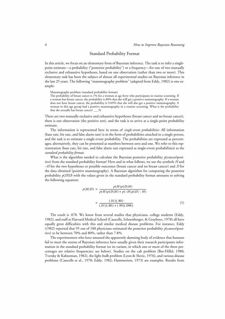
In this article, we focus on an elementary form of Bayesian inference. The task is to infer a single-point estimate—a probability (“posterior probability”) or a frequency—for one of two mutuallyexclusive and exhaustive hypotheses, based on one observation (rather than two or more). Thiselementary task has been the subject of almost all experimental studies on Bayesian inference inthe last 25 years. The following “mammography problem” (adapted from Eddy, 1982) is one ex-ample:
Mammography problem (standard probability format)The probability of breast cancer is 1% for a woman at age forty who participates in routine screening. Ifa woman has breast cancer, the probability is 80% that she will get a positive mammography. If a womandoes not have breast cancer, the probability is 9.69% that she will also get a positive mammography. Awoman in this age group had a positive mammography in a routine screening. What is the probabilitythat she actually has breast cancer? ___%
There are two mutually exclusive and exhaustive hypotheses (breast cancer and no breast cancer),there is one observation (the positive test), and the task is to arrive at a single-point probabilityestimate.
The information is represented here in terms of
single-event probabilities:
All information(base rate, hit rate, and false alarm rate) is in the form of probabilities attached to a single person,and the task is to estimate a single-event probability. The probabilities are expressed as percent-ages; alternatively, they can be presented as numbers between zero and one. We refer to this rep-resentation (base rate, hit rate, and false alarm rate expressed as single-event probabilities) as the
standard probability format.
What is the algorithm needed to calculate the Bayesian posterior probability
p
(cancer|posi-tive) from the standard probability format? Here and in what follows, we use the symbols
H
and
–H
for the two hypotheses or possible outcomes (breast cancer and no breast cancer) and
D
forthe data obtained (positive mammography). A Bayesian algorithm for computing the posteriorprobability
p
(
H|D
) with the values given in the standard probability format amounts to solvingthe following equation:
(1)
The result is .078. We know from several studies that physicians, college students (Eddy,1982), and staff at Harvard Medical School (Casscells, Schoenberger, & Grayboys, 1978) all haveequally great difficulties with this and similar medical disease problems. For instance, Eddy(1982) reported that 95 out of 100 physicians estimated the posterior probability
p
(cancer|posi-tive) to be between 70% and 80%, rather than 7.8%.
The experimenters who have amassed the apparently damning body of evidence that humansfail to meet the norms of Bayesian inference have usually given their research participants infor-mation in the standard probability format (or its variant, in which one or more of the three per-centages are relative frequencies; see below). Studies on the cab problem (Bar-Hillel, 1980;Tversky & Kahneman, 1982), the light-bulb problem (Lyon & Slovic, 1976), and various diseaseproblems (Casscells et al., 1978; Eddy, 1982; Hammerton, 1973) are examples. Results from
p H D( )p H( ) p D H( )
p H( ) p D H( ) p H–( ) p D H–( )+-----------------------------------------------------------------------------------=
.01( ) .80( ).01( ) .80( ) .99( ) .096( )+
----------------------------------------------------------- .=
Gerd Gigerenzer and Ulrich Hoffrage
5
these and other studies have generally been taken as evidence that the human mind does not rea-son with Bayesian algorithms. Yet this conclusion is not warranted, as explained before. Onewould be unable to detect a Bayesian algorithm within a system by feeding it information in arepresentation that does not match the representation with which the algorithm works.
In the last few decades, the standard probability format has become a common way to com-municate information ranging from medical and statistical textbooks to psychological experi-ments. But we should keep in mind that it is only one of many mathematically equivalent waysof representing information; it is, moreover, a recently invented notation. Neither the standardprobability format nor Equation 1 was used in Bayes’ (1763) original essay. Indeed, the notionof “probability” did not gain prominence in probability theory until one century after the math-ematical theory of probability was invented (Gigerenzer, Swijtink, Porter, Daston, Beatty, &Krüger, 1989). Percentages became common notations only during the 19th century (mainly forinterest and taxes), after the metric system was introduced during the French Revolution. Thus,probabilities and percentages took millennia of literacy and numeracy to evolve; organisms didnot acquire information in terms of probabilities and percentages until very recently. How didorganisms acquire information before that time? We now investigate the links between informa-tion representation and information acquisition.
Natural Sampling of Frequencies
Evolutionary theory asserts that the design of the mind and its environment evolve in tandem.Assume—pace Gould—that humans have evolved cognitive algorithms that can perform statis-tical inferences. These algorithms, however, would not be tuned to probabilities or percentagesas input format, as explained before. For what information format were these algorithms de-signed? We assume that as humans evolved, the “natural” format was
frequencies
as actually ex-perienced in a series of events, rather than probabilities or percentages (Cosmides & Tooby, inpress; Gigerenzer, 1991b, 1993a). From animals to neural networks, systems seem to learn aboutcontingencies through sequential encoding and updating of event frequencies (Brunswik, 1939;Gallistel, 1990; Hume, 1739/1951; Shanks, 1991). For instance, research on foraging behaviorindicates that bumblebees, ducks, rats, and ants behave as if they were good intuitive statisticians,highly sensitive to changes in frequency distributions in their environments (Gallistel, 1990;Real, 1991; Real & Caraco, 1986). Similarly, research on frequency processing in humans indi-cates that humans, too, are sensitive to frequencies of various kinds, including frequencies ofwords, single letters, and letter pairs (e.g., Barsalou & Ross, 1986; Hasher & Zacks, 1979; Hintz-man, 1976; Sedlmeier, Hertwig, & Gigerenzer, 1995).
The sequential acquisition of information by updating event frequencies
without
artificiallyfixing the marginal frequencies (e.g., of disease and no-disease cases) is what we refer to as
naturalsampling
(Kleiter, 1994). Brunswik’s (1955) “representative sampling” is a special case of naturalsampling. In contrast, in experimental research the marginal frequencies are typically fixed a pri-ori. For instance, an experimenter may want to investigate 100 people with disease and a controlgroup of 100 people without disease. This kind of sampling with fixed marginal frequencies isnot what we refer to as natural sampling.
The evolutionary argument that cognitive algorithms were designed for frequency informa-tion, acquired through natural sampling, has implications for the computations an organismneeds to perform when making Bayesian inferences.Here is the question to be answered: Assumean organism acquires information about the structure of its environment by the natural sampling
6
How to Improve Bayesian Reasoning
of frequencies. What computations would the organism need to perform to draw inferences theBayesian way?
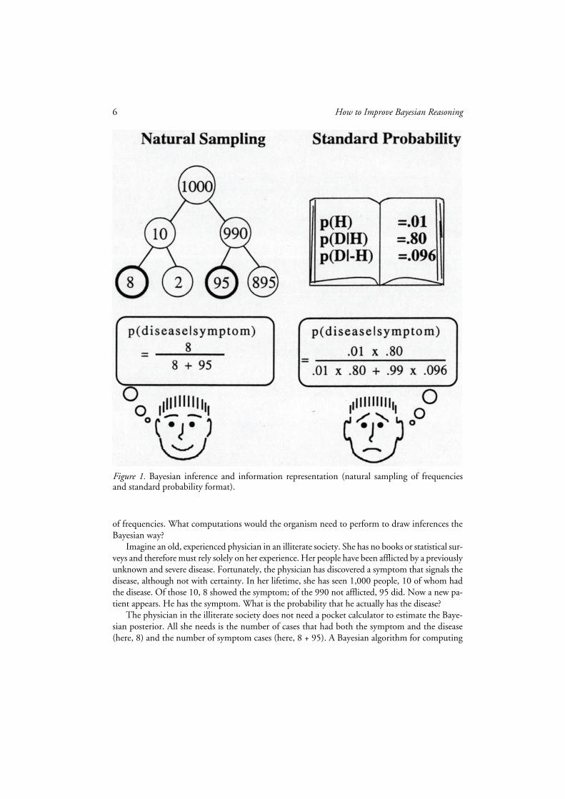
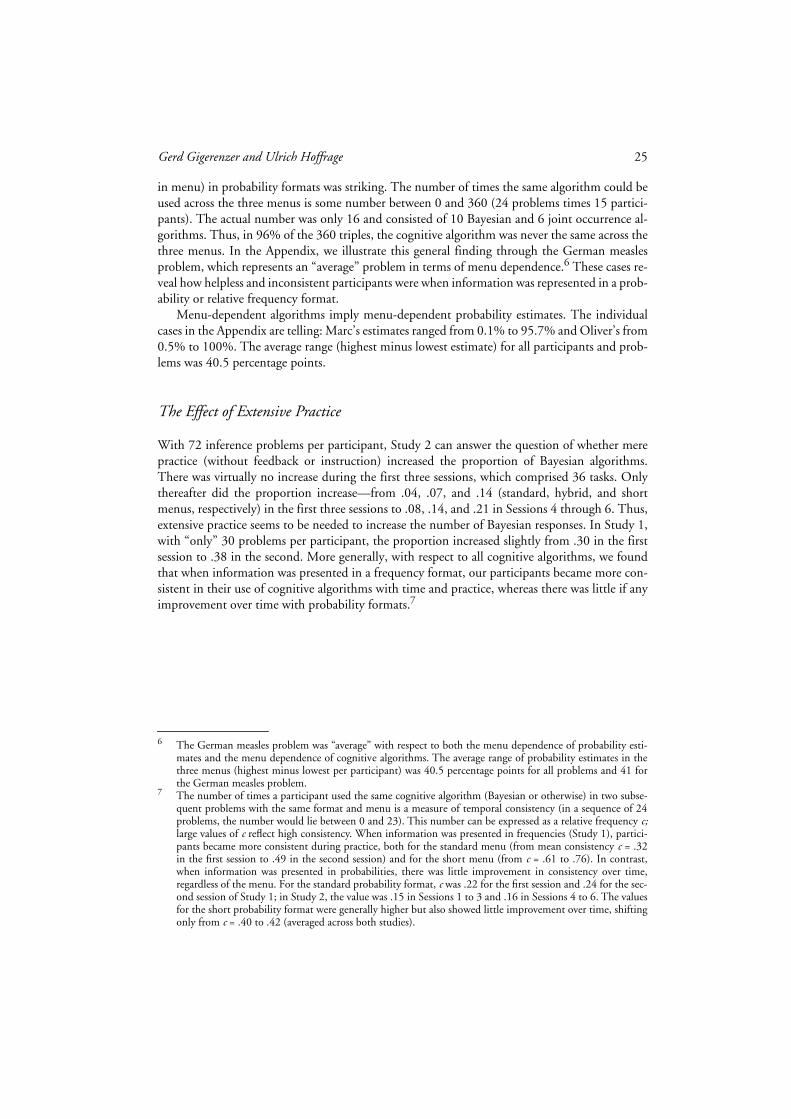
Imagine an old, experienced physician in an illiterate society. She has no books or statistical sur-veys and therefore must rely solely on her experience. Her people have been afflicted by a previouslyunknown and severe disease. Fortunately, the physician has discovered a symptom that signals thedisease, although not with certainty. In her lifetime, she has seen 1,000 people, 10 of whom hadthe disease. Of those 10, 8 showed the symptom; of the 990 not afflicted, 95 did. Now a new pa-tient appears. He has the symptom. What is the probability that he actually has the disease?
The physician in the illiterate society does not need a pocket calculator to estimate the Baye-sian posterior. All she needs is the number of cases that had both the symptom and the disease(here, 8) and the number of symptom cases (here, 8 + 95). A Bayesian algorithm for computing
Figure 1.
Bayesian inference and information representation (natural sampling of frequenciesand standard probability format).

Gerd Gigerenzer and Ulrich Hoffrage
7
the posterior probability
p
(
H
|
D
) from the frequency format (see Figure 1, left side) requires solv-ing the following equation:
(2)
where
d
&
h
(
d
ata and
h
ypothesis) is the number of cases with symptom and disease, and
d
&
–h
is the number of cases having the symptom but lacking the disease. The physician does not needto keep track of the base rate of the disease. Her modern counterpart, the medical student whostruggles with single-event probabilities presented in medical textbooks, may on the other handhave to rely on a calculator and end up with little understanding of the result (see Figure 1, rightside).
2
Henceforth, when we use the term
frequency format,
we always refer to frequencies as de-fined by the natural sampling tree in Figure 1.
Comparison of Equations 1 and 2 leads to our first theoretical result:
Result 1: Computational demands. Bayesian algorithms are computationally simpler when infor-mation is encoded in a frequency format rather than a standard probability format.
By “computa-tionally simpler” we mean that (a) fewer operations (multiplication, addition, or division) needto be performed in Equation 2 than Equation 1, and (b) the operations can be performed on nat-ural numbers (absolute frequencies) rather than fractions (such as percentages).
Equations 1 and 2 are mathematically equivalent formulations of Bayes’ theorem. Both pro-duce the same result,
p
(
H
|
D
) = .078. Equation 1 is a standard version of Bayes’ theorem in today’stextbooks in the social sciences, whereas Equation 2 corresponds to Thomas Bayes’ (1763) orig-inal “Proposition 5” (see Earman, 1992).
Equation 2 implies three further (not independent) theoretical results concerning the estima-tion of a Bayesian posterior probability
p
(
H
|
D
) in frequency formats (Kleiter, 1994).
Result 2: Attentional demands. Only two kinds of information need to be attended to in naturalsampling: the absolute frequencies d & h and d & –h (or, alternately, d & h and d, where d is the sumof the two frequencies).
An organism does not need to keep track of the whole tree in Figure 1, butonly of the two pieces of information contained in the bold circles. These are the hit and falsealarm
frequencies
(not to be confused with hit and false alarm
rates
).
Result 3: Base rates need not be attended to.
Neglect of base rates is perfectly rational in naturalsampling. For instance, our physician does not need to pay attention to the base rate of the disease(10 out of 1,000; see Figure 1).
Result 4: Posterior distributions can be computed.
Absolute frequencies can carry more informa-tion than probabilities. Information about the sample size allows inference beyond single-pointestimates, such as the computation of posterior distributions, confidence intervals for posteriorprobabilities, and second-order probabilities (Kleiter, 1994; Sahlin, 1993). In this article, how-ever, we focus only on single-point estimation.
For the design of the experiments reported below, it is important to note that the Bayesianalgorithms (Equations 1 and 2) work on the final tally of frequencies (see Figure 1), not on thesequential record of updated frequencies. Thus, the same four results still hold even if nothingbut the final tally is presented to the participants in an experiment.
2
This clinical example illustrates that the standard probability format is a convention rather than a necessity.Clinical studies often collect data that have the structure of frequency trees as in Figure 1. Such informationcan always be represented in frequencies as well as probabilities.
p H D( ) d & hd & h d & h–+-------------------------------------- 8
8 95+--------------- ,==
8
How to Improve Bayesian Reasoning
Information Format and Menu
We propose to distinguish two aspects of information representation,
information format
and
in-formation menu.
The standard probability format has a
probability format,
whereas a
frequency for-mat
is obtained by natural sampling. However, as the second result (attentional demands) shows,there is another difference. The standard probability format displays three pieces of information,whereas two are sufficient in natural sampling. We use the term
information menu
to refer to themanner in which information is segmented into pieces within any format. The standard proba-bility format displays the three pieces
p
(
H
),
p
(D|
H
), and
p
(D|
–H
) (often called base rate, hit rate,and false alarm rate, respectively). We refer to this as the
standard menu.
Natural sampling yieldsa more parsimonious menu with only two pieces of information,
d
&
h
and
d
&
–h
(or alterna-tively,
d
&
h
and
d
). We call this the short menu. So far we have introduced the probability format with a standard menu and the frequency
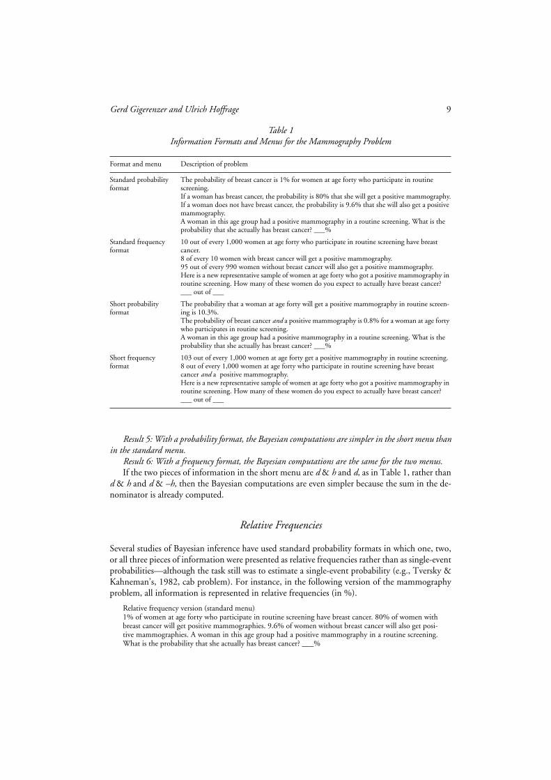
format with a short menu. However, information formats and menus can be completely crossed.For instance, if we replace the probabilities in the standard probability format with frequencies,we get a standard menu with a frequency format, or the standard frequency format. Table 1 usesthe mammography problem to illustrate the four versions that result from crossing the twomenus with the two formats. All four displays are mathematically equivalent in the sense that theylead to the same Bayesian posterior probability. In general, within the same format informationcan be divided into various menus; within the same menu, it can be represented in a range offormats.
To transform the standard probability format into the standard frequency format, we simplyreplaced 1% with “10 out of 1,000,” “80%” with “8 out of 10,” and so on (following the tree inFigure 1) and phrased the task in terms of a frequency estimate. All else went unchanged. Notethat whether the frequency format actually carries information about the sample size (e.g., thatthere were exactly 1,000 women) or not (as in Table 1, where it is said “in every 1,000 women”)makes no difference for Results 1 to 3 because these relate to single-point estimates only (unlikeResult 4).
What are the Bayesian algorithms needed to draw inferences from the two new format-menucombinations? The complete crossing of formats and menus leads to two important results. ABayesian algorithm for the short probability format, that is, the probability format with a shortmenu (as in Table 1), amounts to solving the following equation:
. (3)
This version of Bayes’ theorem is equivalent to Equation 1. The algorithm for computing p(H|D)from Equation 3, however, is computationally simpler than the algorithm for computing p(H|D) fromEquation 1.
What Bayesian computations are needed for the standard frequency format? Equation 2specifies the computations for both the standard and short menus in frequency formats. Thesame algorithm is sufficient for both menus. In the standard frequency format of the mammog-raphy problem, for instance, the expected number of actual breast cancer cases among positivetests is computed as 8/(8 + 95). Thus, we have the following two important theoretical resultsconcerning formats (probability vs. frequency) and menus (standard vs. short):
p H D( )p D&H( )
p D( )-----------------------=
Gerd Gigerenzer and Ulrich Hoffrage 9
Result 5: With a probability format, the Bayesian computations are simpler in the short menu thanin the standard menu.
Result 6: With a frequency format, the Bayesian computations are the same for the two menus.If the two pieces of information in the short menu are d & h and d, as in Table 1, rather than
d & h and d & –h, then the Bayesian computations are even simpler because the sum in the de-nominator is already computed.
Relative Frequencies
Several studies of Bayesian inference have used standard probability formats in which one, two,or all three pieces of information were presented as relative frequencies rather than as single-eventprobabilities—although the task still was to estimate a single-event probability (e.g., Tversky &Kahneman’s, 1982, cab problem). For instance, in the following version of the mammographyproblem, all information is represented in relative frequencies (in %).
Relative frequency version (standard menu) 1% of women at age forty who participate in routine screening have breast cancer. 80% of women withbreast cancer will get positive mammographies. 9.6% of women without breast cancer will also get posi-tive mammographies. A woman in this age group had a positive mammography in a routine screening.What is the probability that she actually has breast cancer? ___%
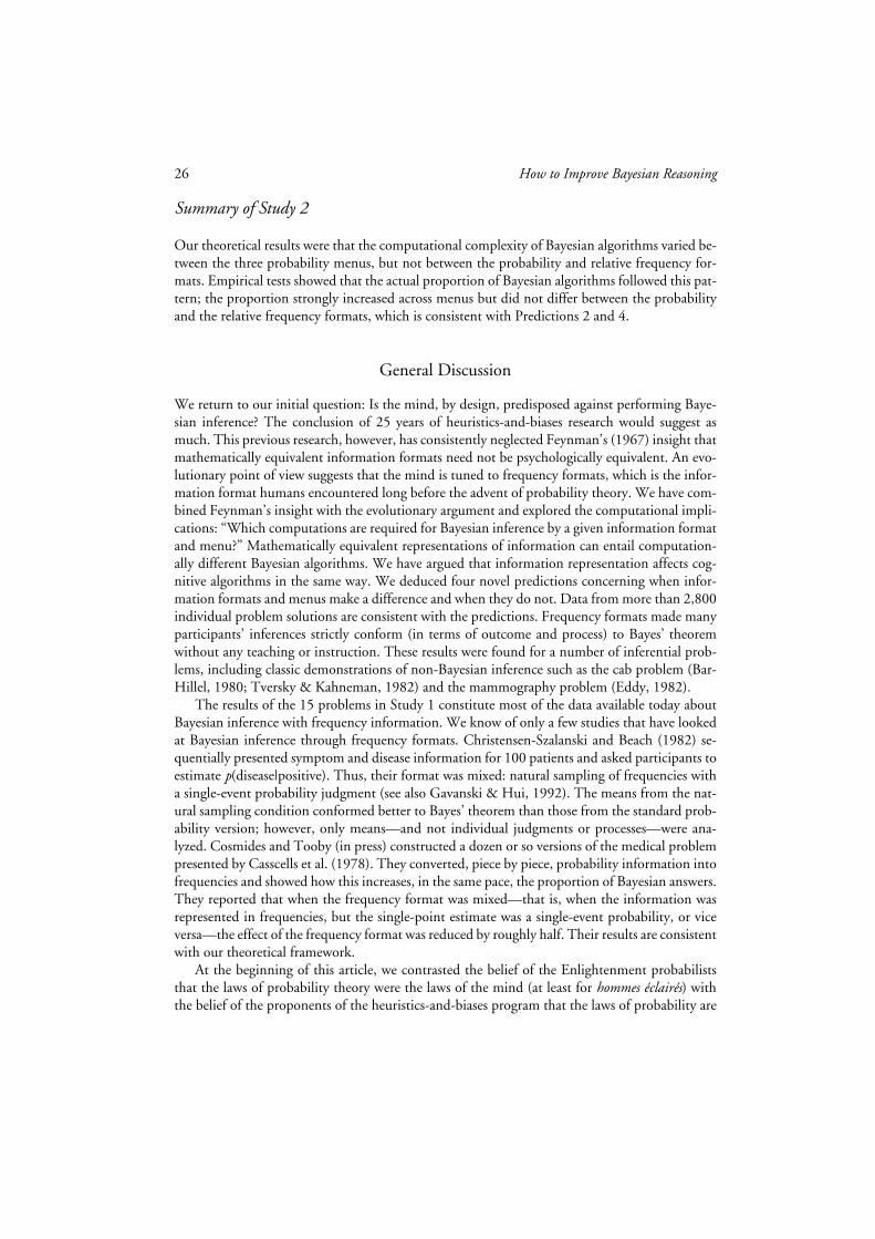
Table 1Information Formats and Menus for the Mammography Problem
Format and menu Description of problem
Standard probability format
The probability of breast cancer is 1% for women at age forty who participate in routine screening.If a woman has breast cancer, the probability is 80% that she will get a positive mammography.If a woman does not have breast cancer, the probability is 9.6% that she will also get a positive mammography.A woman in this age group had a positive mammography in a routine screening. What is the probability that she actually has breast cancer? ___%
Standard frequency format
10 out of every 1,000 women at age forty who participate in routine screening have breast cancer.8 of every 10 women with breast cancer will get a positive mammography.95 out of every 990 women without breast cancer will also get a positive mammography.Here is a new representative sample of women at age forty who got a positive mammography in routine screening. How many of these women do you expect to actually have breast cancer? ___ out of ___
Short probability format
The probability that a woman at age forty will get a positive mammography in routine screen-ing is 10.3%.The probability of breast cancer and a positive mammography is 0.8% for a woman at age forty who participates in routine screening.A woman in this age group had a positive mammography in a routine screening. What is the probability that she actually has breast cancer? ___%
Short frequency format
103 out of every 1,000 women at age forty get a positive mammography in routine screening.8 out of every 1,000 women at age forty who participate in routine screening have breast cancer and a positive mammography.Here is a new representative sample of women at age forty who got a positive mammography in routine screening. How many of these women do you expect to actually have breast cancer? ___ out of ___
10 How to Improve Bayesian Reasoning
Is the algorithm needed for relative frequencies computationally equivalent to the algorithm forfrequencies, or to that for probabilities? The relative frequency format does not display the abso-lute frequencies needed for Equation 2. Rather, the numbers are the same as in the probabilityformat, making the Bayesian computation the same as in Equation 1. This yields the followingresult:
Result 7: Algorithms for relative frequency versions are computationally equivalent to those for thestandard probability format.
We tested several implications of Results 1 through 7 (except Result 4) in the studies reportedbelow.
The Format of the Single-Point Estimate
Whether estimates relate to single events or frequencies has been a central issue within probabilitytheory and statistics since the decline of the classical interpretation of probability in the 1830sand 1840s. The question has polarized subjectivists and frequentists, additionally subdividingfrequentists into moderate frequentists, such as R. A. Fisher (1955), and strong frequentists, suchas J. Neyman (Gigerenzer et al., 1989). A single-point estimate can be interpreted as a probabilityor a frequency. For instance, clinical inference can be about the probability that a particular per-son has cancer or about the frequency of cancer in a new sample of people. Foraging (Simon,1956; Stephens & Krebs, 1986) provides an excellent example of a single-point estimate reason-ably being interpreted as a frequency. The foraging organism is interested in making inferencesthat lead to satisfying results in the long run. Will it more often find food if it follows Cue X orCue Y? Here the single-point estimate can be interpreted as an expected frequency for a new sam-ple. In the experimental research of the past two decades, participants were almost always re-quired to estimate a single-event probability. But this need not be. In the experiments reportedbelow, we asked people both for single-event probability and frequency estimates.
To summarize, mathematically equivalent information need not be computationally and psy-chologically equivalent. We have shown that Bayesian algorithms can depend on informationformat and menu, and we derived several specific results for when algorithms are computationallyequivalent and when they are not.
Cognitive Algorithms for Bayesian Inference
How might the mind draw inferences that follow Bayes’ theorem? Surprisingly, this questionseems rarely to have been posed. Psychological explanations typically were directed at “irrational”deviations between human inference and the laws of probability; the “rational” seems not to havedemanded an explanation in terms of cognitive processes. The cognitive account of probabilisticreasoning by Piaget and Inhelder (1951/1975), as one example, stops at the precise moment theadolescent turns “rational,” that is, reaches the level of formal operations.
We propose three classes of cognitive algorithm for Bayesian inference: first, the algorithmscorresponding to Equations 1 through 3; second, pictorial or graphical analogs of Bayes’ theo-rem, as anticipated by Bayes’ (1763) billiard table; and third, shortcuts that simplify the Bayesiancomputations in Equations 1 through 3.

Gerd Gigerenzer and Ulrich Hoffrage 11
Pictorial Analogs
We illustrate pictorial analogs and shortcut algorithms by drawing on actual performance fromthe studies reported below, in which none of the participants was familiar with Bayes’ theorem.The German measles problem (in standard probability format and with the numerical informa-tion given in Study 2) serves as our example.
German measles during early pregnancy can cause severe prenatal damage in the child. Therefore, preg-nant women are routinely tested for German measles infection. In one such test, a pregnant woman isfound to be infected. In order best to advise this woman what to do, the physician first wants to deter-mine the probability of severe prenatal damage in the child if a mother has German measles during earlypregnancy. The physician has the following information: The probability of severe prenatal damage in achild is 0.5%. The probability that a mother had German measles during early pregnancy if her child hassevere prenatal damage is 40%. The probability that a mother had German measles during early preg-nancy if her child does not have severe prenatal damage is 0.01%. What is the probability of severe pre-natal damage in the child if the mother has German measles during early pregnancy? ___%
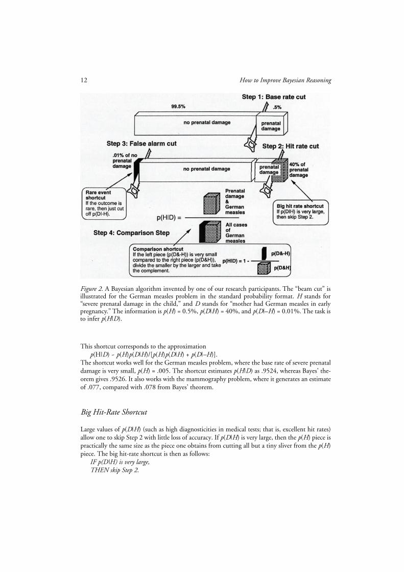
The “beam analysis” (see Figure 2) is a pictorial analog of Bayes’ theorem developed by one ofour research participants. This individual represented the class of all possible outcomes (child hassevere prenatal damage and child does not have severe prenatal damage) by a beam. He drew in-ferences (here, about the probability that the child has severe prenatal damage) by cutting off twopieces from each end of the beam and comparing their size. His algorithm was as follows:
Step 1: Base rate cut. Cut off a piece the size of the base rate from the right end of the beam.Step 2: Hit rate cut. From the right part of the beam (base rate piece), cut off a proportion p(D|H).Step 3: False alarm cut. From the left part of the beam, cut off a proportion p(D|–H).Step 4: Comparison. The ratio of the right piece to both pieces is the posterior probability.
This algorithm amounts to Bayes’ theorem in the form of Equation 1.
Shortcut Algorithms: Probability Format
We have observed in our experiments three elementary shortcuts and several combinations there-of. For instance, by ignoring small “slices,” one can simplify the computation without much lossof accuracy, which is easily compensated for by the fact that less computation means a reducedchance of computational errors. We illustrate these shortcuts using the beam analysis (seeFigure 2). However, these shortcuts are not restricted to pictorial analogs, and they were used bymany of our participants.
Rare-Event Shortcut
Rare events—that is, outcomes with small base rates, such as severe prenatal damage—enable sim-plification of the Bayesian inference with little reduction in accuracy. If an event is rare, that is, ifp(H) is very small, and p(–H) is therefore close to 1.0, then p(D|–H)p(–H) can be approximatedby p(D|–H). That is, instead of cutting the proportion p(D|–H) of the left part of the beam (Step 3),it is sufficient to cut a piece of absolute size p(D|–H). The rare-event shortcut (see Figure 2) is asfollows:
IF the event is rare,THEN simplify Step 3: Cut a piece of absolute size p(D|–H).
12 How to Improve Bayesian Reasoning
This shortcut corresponds to the approximation p(H|D) ~ p(H)p(D|H)/[p(H)p(D|H) + p(D|–H)].
The shortcut works well for the German measles problem, where the base rate of severe prenataldamage is very small, p(H) = .005. The shortcut estimates p(H|D) as .9524, whereas Bayes’ the-orem gives .9526. It also works with the mammography problem, where it generates an estimateof .077, compared with .078 from Bayes’ theorem.
Big Hit-Rate Shortcut
Large values of p(D|H) (such as high diagnosticities in medical tests; that is, excellent hit rates)allow one to skip Step 2 with little loss of accuracy. If p(D|H) is very large, then the p(H) piece ispractically the same size as the piece one obtains from cutting all but a tiny sliver from the p(H)piece. The big hit-rate shortcut is then as follows:
IF p(D|H) is very large,THEN skip Step 2.
Figure 2. A Bayesian algorithm invented by one of our research participants. The “beam cut” isillustrated for the German measles problem in the standard probability format. H stands for“severe prenatal damage in the child,” and D stands for “mother had German measles in earlypregnancy.” The information is p(H) = 0.5%, p(D|H) = 40%, and p(D|–H) = 0.01%. The task isto infer p(H|D).
Gerd Gigerenzer and Ulrich Hoffrage 13
This shortcut corresponds to the approximationp(H|D) ~ p(H)/ [p(H) + p(–H)p(D|–H)].
The big hit-rate shortcut would not work as well as the rare-event shortcut in the German measlesproblem because p(D|H) is only .40. Nevertheless, the shortcut estimate is only a few percentagepoints removed from that obtained with Bayes‘ theorem (.980 instead of .953). The big hit-rateshortcut works well, to offer one instance, in medical diagnosis tasks where the hit rate of a testis high (e.g., around .99 as in HIV tests).
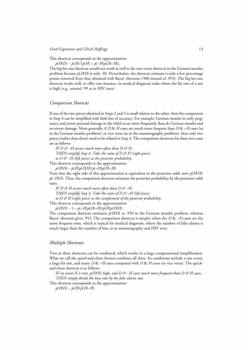
Comparison Shortcut
If one of the two pieces obtained in Steps 2 and 3 is small relative to the other, then the comparisonin Step 4 can be simplified with little loss of accuracy. For example, German measles in early preg-nancy and severe prenatal damage in the child occur more frequently than do German measles andno severe damage. More generally, if D & H cases are much more frequent than D & –H cases (asin the German measles problem), or vice versa (as in the mammography problem), then only twopieces (rather than three) need to be related in Step 4. The comparison shortcuts for these two casesare as follows:
IF D & –H occurs much more often than D & H,THEN simplify Step 4: Take the ratio of D & H (right piece) to D & –H (left piece) as the posterior probability.
This shortcut corresponds to the approximationp(H|D) ~ p(H)p(D|H)/p(–H)p(D|–H).
Note that the right side of this approximation is equivalent to the posterior odds ratio p(H|D)/p(–H|D). Thus, the comparison shortcut estimates the posterior probability by the posterior oddsratio.
IF D & H occurs much more often than D & –H,THEN simplify Step 4: Take the ratio of D & –H (left piece)to D & H (right piece) as the complement of the posterior probability.
This shortcut corresponds to the approximationp(H|D) ~ 1 – p(–H)p(D|–H)/p(H)p(D|H).
The comparison shortcut estimates p(H|D) as .950 in the German measles problem, whereasBayes’ theorem gives .953. The comparison shortcut is simpler when the D & –H cases are themore frequent ones, which is typical for medical diagnosis, where the number of false alarms ismuch larger than the number of hits, as in mammography and HIV tests.
Multiple Shortcuts
Two or three shortcuts can be combined, which results in a large computational simplification.What we call the quick-and-clean shortcut combines all three. Its conditions include a rare event,a large hit rate, and many D & –H cases compared with D & H cases (or vice versa). The quick-and-clean shortcut is as follows:
IF an event H is rare, p(D|H) high, and D & –H cases much more frequent than D & H cases,THEN simply divide the base rate by the false alarm rate.
This shortcut corresponds to the approximationp(H|D) ~ p(H)/p(D|–H).

14 How to Improve Bayesian Reasoning
The conditions of the quick-and-clean shortcut seem to be not infrequently satisfied. Considerroutine HIV testing: According to present law, the U.S. immigration office makes an HIV test acondition sine qua non for obtaining a green card. Mr. Quick has applied for a green card andwonders what a positive test result indicates. The information available is a base rate of .002, ahit rate of .99, and a false alarm rate of .02; all three conditions for the quick-and-clean shortcutare thus satisfied. Mr. Quick computes .002/.02 = .10 as an estimate of the posterior probabilityof actually being infected with the HIV virus if he tests positive. Bayes’ theorem results in .09.The shortcut is therefore an excellent approximation. Alternately, if D & H cases are more fre-quent, then the quick-and-clean shortcut is to divide the false alarm rate by the base rate and touse this as an estimate for 1 – p(H|D). In the mammography and German measles problems,where the conditions are only partially satisfied, the quick-and-clean shortcut still leads to sur-prisingly good approximations. The posterior probability of breast cancer is estimated at .01/.096, which is about .10 (compared with .078), and the posterior probability of severe prenataldamage is estimated as .98 (compared with .953).
Shortcuts: Frequency Format
Does the standard frequency format invite the same shortcuts? Consider the inference aboutbreast cancer from a positive mammography, as illustrated in Figure 1. Would the rare-eventshortcut facilitate the Bayesian computations? In the probability format, the rare-event shortcutuses p(D|–H) to approximate p(–H)p(D|–H); in the frequency format, the latter corresponds tothe absolute frequency 95 (d & –h) and no approximation is needed. Thus, a rare-event shortcutis of no use and would not simplify the Bayesian computation in frequency formats. The samecan be shown for the big hit-rate shortcut for the same reason. The comparison shortcut, how-ever, can be applied in the frequency format:
IF d & –h occurs much more often than d & h,THEN compute d & h/d &–h.
The condition and the rationale are the same as in the probability format.To summarize, we proposed three classes of cognitive algorithms underlying Bayesian infer-
ence: (a) algorithms that satisfy Equations 1 through 3; (b) pictorial analogs that work with op-erations such as “cutting” instead of multiplying (Figure 2); and (c) three shortcuts that approx-imate Bayesian inference well when certain conditions hold.
Predictions
We now derive several predictions from the theoretical results obtained. The predictions specifyconditions that do and do not make people reason the Bayesian way. The predictions should holdindependently of whether the cognitive algorithms follow Equations 1 through 3, whether theyare pictorial analogs of Bayes’ theorem, or whether they include shortcuts.
Prediction 1: Frequency formats elicit a substantially higher proportion of Bayesian algorithmsthan probability formats. This prediction is derived from Result 1, which states that the Bayesianalgorithm is computationally simpler in frequency formats.3
Prediction 2: Probability formats elicit a larger proportion of Bayesian algorithms for the shortmenu than for the standard menu. This prediction is deduced from Result 5, which states that with

Gerd Gigerenzer and Ulrich Hoffrage 15
a probability format, the Bayesian computations are simpler in the short menu than in the stan-dard menu.
Prediction 3: Frequency formats elicit the same proportion of Bayesian algorithms for the twomenus. This prediction is derived from Result 6, which states that with a frequency format, theBayesian computations are the same for the two menus.
Prediction 4: Relative frequency formats elicit the same (small) proportion of Bayesian algorithmsas probability formats. This prediction is derived from Result 7, which states that the Bayesian al-gorithms are computationally equivalent in both formats.
Operational Criteria for IdentifyingCognitive Algorithms
The data we obtained for each of several thousand problem solutions were composed of a partic-ipant’s (a) probability or frequency estimate and (b) on-line protocol (“write aloud” protocol) ofhis or her reasoning. Data type (a) allowed for an outcome analysis, as used exclusively in mostearlier studies on Bayesian inference, whereas data type (b) allowed additionally for a processanalysis.
Double Check: Outcome and Process
We classified an inferential process as a Bayesian algorithm only if (a) the estimated probabilityor frequency was exactly the same as the value calculated from applying Bayes’ theorem to theinformation given (outcome criterion), and (b) the on-line protocol specified that one of theBayesian computations defined by Equations 1 through 3 or one (or several) of the Bayesianshortcut algorithms was used, either by means of calculation or pictorial representation (processcriterion). We applied the same strict criteria to identify non-Bayesian cognitive algorithms.
Outcome: Strict Rounding Criterion
By the phrase “exactly the same” in the outcome criterion, we mean the exact probability or fre-quency, with exceptions made for rounding up or down to the next full percentage point (e.g.,in the German measles problem, where rounding the probability of 95.3% down or up to a fullpercentage point results in 95% or 96%). If, for example, the on-line protocol showed that a par-ticipant in the German measles problem had used the rare-event shortcut and the answer was95% or 96% (by rounding), this inferential process was classified as a Bayesian algorithm. Esti-mates below or above were not classified as Bayesian algorithms: If, for example, another partic-ipant in the same problem used the big hit-rate shortcut (where the condition for this shortcut is
3 At the point when we introduced Result 1, we had dealt solely with the standard probability format and theshort frequency format. However, Prediction 1 also holds when we compare formats across both menus. Thisis the case because (a) the short menu is computationally simpler in the frequency than in the probabilityformat, because the frequency format involves calculations with natural numbers and the probability formatwith fractions, and (b) with a frequency format, the Bayesian computations are the same for the two menus(Result 6).

16 How to Improve Bayesian Reasoning
not optimally satisfied) and accordingly estimated 98%, this was not classified as a Bayesian al-gorithm. Cases of the latter type ended up in the category of “less frequent algorithms.” This ex-ample illustrates the strictness of the joint criteria. The strict rounding criterion was applied tothe frequency format in the same way as to the probability format.
When a participant answered with a fraction—such as that resulting from Equation 3—with-out performing the division, this was treated as if she or he had performed the division. We didnot want to evaluate basic arithmetic skills. Similarly, if a participant arrived at a Bayesian equa-tion but made a calculation error in the division, we ignored the calculation error.
Process: “Write Aloud” Protocols
Statistical reasoning often involves pictorial representations as well as computations. Neither areeasily expressed verbally, as in “think aloud” methods. Pictorial representations and computa-tions consequently are usually expressed by drawing and writing down equations and calcula-tions. We designed a “write aloud” technique for tracking the reasoning process without askingthe participant to talk aloud either during or after the task.
The “write aloud” method consisted of the following steps. First, participants were instructedto record their reasoning unless merely guessing the answer. We explained that a protocol maycontain a variety of elements, such as diagrams, pictures, calculations, or whatever other tools onemay use to find a solution. Each problem was on a separate page, which thus allowed ample spacefor notes, drawings, and calculations. Second, after a participant had completed a problem, he orshe was asked to indicate whether the answer was based on a calculation or on a guess. Third,when a “write aloud” protocol was unreadable or the process that generated the probability esti-mate was unclear, and the participant had indicated that the given result was a calculation, thenhe or she was interviewed about the particular problem after completing all tasks. This happenedonly a few times. If a participant could not immediately identify what his or her notes meant, wedid not inquire further.
The “write aloud” method avoids two problems associated with retrospective verbal reports:That memory of the cognitive algorithms used may have faded by the time of a retrospective re-port (Ericsson & Simon, 1984) and that participants may have reported how they believe theyought to have thought rather than how they actually thought (Nisbett & Wilson, 1977).
We used the twin criteria of outcome and process to cross-check outcome by process and viceversa. The outcome criterion prevents a shortcut algorithm from being classified as a Bayesianalgorithm when the precondition for the shortcut is not optimally satisfied. The process criterionprotects against the opposite error, that of inferring from a probability judgment that a personactually used a Bayesian algorithm when he or she did not.
We designed two studies to identify the cognitive algorithms and test the predictions. Study 1was designed to test Predictions 1, 2, and 3.
Gerd Gigerenzer and Ulrich Hoffrage 17
Study 1: Information Formats and Menus
Method
Participants
Sixty students, 21 men and 39 women from 10 disciplines (predominantly psychology) from theUniversity of Salzburg, Austria, were paid for their participation. The median age was 21 years.None of the participants was familiar with Bayes’ theorem.
Participants were studied individually or in small groups of 2 or 3 (in two cases, 5). We in-formed participants that they would need approximately 1 hr for each session but that they couldhave more time if necessary. On the average, students worked 73 min in the first session (range= 25–180 min) and 53 min in the second (range = 30–120 min).
Procedure
We used two formats, probability and frequency, and two menus, standard and short. The twoformats were crossed with the two menus, so four versions were constructed for each problem.There were 15 problems, including the mammography problem (Eddy, 1982; see Table 1), thecab problem (Tversky & Kahneman, 1982), and a short version of Ajzen’s (1977) economicsproblem. The four versions of each problem were constructed in the same way as explained beforewith the mammography problem (see Table 1).4 In the frequency format, participants were al-ways asked to estimate the frequency of “h out of d”; in the probability format, they were alwaysasked to estimate the probability p(H|D). Table 2 shows for each of the 15 problems the infor-mation given in the standard frequency format; the information specified in the other three ver-sions can be derived from that.
Participants were randomly assigned to two groups, with the members of both answeringeach of the 15 problems in two of the four versions. One group received the standard probabilityformat and the short frequency format; the other, the standard frequency format and the shortprobability format. Each participant thus worked on 30 tasks. There were two sessions, one weekapart, with 15 problems each. Formats and menus were distributed equally over the sessions. Thetwo versions of one problem were always given in different sessions. The order of the problemswas determined randomly, and two different random orders were used within each group.
Results
Bayesian Algorithms
Prediction 1: Frequency formats elicit a substantially higher proportion of Bayesian algorithms thanprobability formats. Do frequency formats foster Bayesian reasoning? Yes. Frequency formats elic-
4 If the Y number in “X out of Y” was large and odd, such as 9,950, we rounded the number to a close, moresimple number, such as 10,000. The German measles problem is an example. This made practically no dif-ference for the Bayesian calculation and was meant to prevent participants from being puzzled by odd Ynumbers.

18 How to Improve Bayesian Reasoning
ited a substantially higher proportion of Bayesian algorithms than probability formats: 46% inthe standard menu and 50% in the short menu. Probability formats, in contrast, elicited 16%and 28%, for the standard menu and the short menu, respectively. These proportions of Bayesianalgorithms were obtained by the strict joint criteria of process and outcome and held fairly stableacross 15 different inference problems. Note that 50% Bayesian algorithms means 50% of all an-swers, and not just of those answers where a cognitive algorithm could be identified. The per-centage of identifiable cognitive algorithms across all formats and menus was 84%.
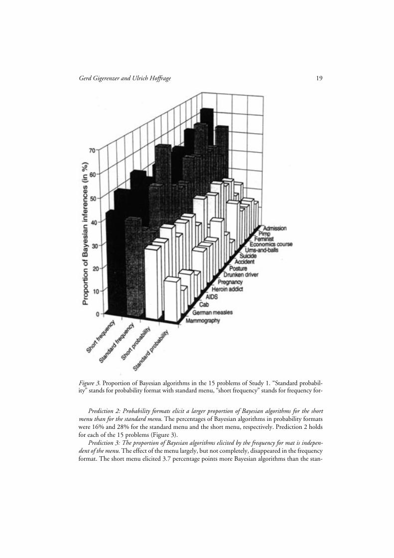
Figure 3 shows the proportions of Bayesian algorithms for each of the 15 problems. The in-dividual problems mirror the general result. For each problem, the standard probability formatelicited the smallest proportion of Bayesian algorithms. Across formats and menus, in every prob-lem Bayesian algorithms were the most frequent.
The comparison shortcut was used quite aptly in the standard frequency format, that is, onlywhen the precondition of the algorithm was satisfied to a high degree. It was most often used inthe suicide problem, in which the ratio between D & H cases and D & –H cases was smallest(Table 2), that is, in which the precondition was best satisfied. Here, 9 out of 30 participants usedthe comparison shortcut (and 5 participants used the Bayesian algorithm without a shortcut). Inall 20 instances where the shortcut was used, 17 satisfied the strict outcome criterion, and theremaining 3 were accurate to within 4 percentage points.
Because of the strict rounding criterion, the numerical estimates of the participants using aBayesian algorithm can be directly read from Table 2. For instance, in the short frequency versionof the mammography problem, 43.3% of participants (see Figure 3) came up with a frequencyestimate of 8 out of 103 (or another value equivalent to 7.8%, or within 7% and 8%).
The empirical result in Figure 3 is consistent with the theoretical result that frequency for-mats can be handled by Bayesian algorithms that are computationally simpler than those requiredby probability formats.
Table 2Information Given and Bayesian Solutions for the 15 Problems in Study 1
Task: Estimate p(H|D) Information (standard frequency format)1 Bayes2
H D H D|H D|–H p(H|D)
Breast cancerPrenatal damage in childBlue cabAIDSHeroin addictPregnantCar accidentBad posture in childAccident on way to schoolCommiting suicideRed ballChoosing course in economicsActive feministPimpAdmission to school
Mammography positiveGerman measles in motherEyewitness says “blue”HIV test positiveFresh needle prickPregnancy test positiveDriver drunkHeavy books carried dailyChild lives in urban areaProfessorMarked with starCareer orientedBank tellerWearing a RolexParticular placement test result
102115
1001020
1005030
240400300
5,00050
360
1,00010,000
1001,000,000
100,0001,000
10,0001,0001,000
1,000,000500
1,000100,000
1,000,0001,000
81012
100101955202736
3002102040
270
102115
1001020
1005030
240400300
5,00050
360
955017
1,000190
5500190388
120,00025
3502,000
500128
99010,000
851,000,000
100,000980
9,900950970
1,000,000100700
95,0001,000,000
640
7.7716.7041.389.095.00
79.179.919.526.510.03
92.3137.500.997.41
67.84
1 The representation of the information is shown only for the standard frequency format (frequency format and standard menu). Theother representations (see Table 1) can be derived from this. The two numbers for each piece of information are connected by an “outof” relation; for example, the information concerning H in the first problem should be read as “10 out of 1,000.”
2 Probabilities are expressed as percentages.
Gerd Gigerenzer and Ulrich Hoffrage 19
Prediction 2: Probability formats elicit a larger proportion of Bayesian algorithms for the shortmenu than for the standard menu. The percentages of Bayesian algorithms in probability formatswere 16% and 28% for the standard menu and the short menu, respectively. Prediction 2 holdsfor each of the 15 problems (Figure 3).
Prediction 3: The proportion of Bayesian algorithms elicited by the frequency for mat is indepen-dent of the menu. The effect of the menu largely, but not completely, disappeared in the frequencyformat. The short menu elicited 3.7 percentage points more Bayesian algorithms than the stan-
Figure 3. Proportion of Bayesian algorithms in the 15 problems of Study 1. “Standard probabil-ity” stands for probability format with standard menu, “short frequency” stands for frequency for-

20 How to Improve Bayesian Reasoning
dard menu. The residual superiority of the short menu could have the following cause: Result 2(attentional demands) states that in natural sampling it is sufficient for an organism to monitoreither the frequencies d & h and d or d & h and d & –h. We have chosen the former pair for theshort menus in our studies and thus reduced the Bayesian computation by one step, that of add-ing up d & h and d & –h to d, which was part of the Bayesian computation in the standard butnot the short menu. This additional computational step is consistent with the small difference inthe proportions of Bayesian algorithms found between the two menus in the frequency formats.
How does the impact of format on Bayesian reasoning compare with that of menu? The effectof the format was about three times larger than that of the menu (29.9 and 21.6 percentage pointsdifference compared with 12.1 and 3.7). Equally striking, the largest percentage of Bayesian al-gorithms in the two probability menus (28%) was considerably smaller than the smallest in thetwo frequency menus (46%).
Non-Bayesian Algorithms
We found three major non-Bayesian cognitive algorithms (see Table 3).Joint occurrence. The most frequent non-Bayesian algorithm was a computation of the joint
occurrence of D and H. Depending on the menu, this involved calculating p(H)p(D|H), or sim-ply “picking” p(H & D) (or the corresponding values for the frequency format). Joint occurrencedoes not neglect base rates; it neglects the false alarm rate in the standard menu and p(D) in theshort menu. Joint occurrence always underestimates the Bayesian posterior unless p(D) = 1. Fromparticipants’ “write aloud” protocols, we learned about a variant, which we call adjusted joint oc-currence, in which the participant starts with joint occurrence and adjusts it slightly (5 or fewerpercentage points).
Fisherian. Not all statisticians are Bayesians. R. A. Fisher, who invented the analysis of vari-ance and promoted significance testing, certainly was not. In Fisher’s (1955) theory of signifi-cance testing, an inference from data D to a null hypothesis Ho is based solely on p(D|Ho), whichis known as the “exact level of significance.” The exact level of significance ignores base rates andfalse alarm rates. With some reluctance, we labeled the second most frequent non-Bayesian algo-rithm—picking p(D|H) and ignoring everything else—“Fisherian.” Our hesitation lay in the factthat it is one thing to ignore everything else besides p(D|H), as Fisher’s significance testing meth-od does, and quite another thing to confuse p(D|H) with p(H|D). For instance, a p value of 1%is often erroneously believed to mean, by both researchers (Oakes, 1986) and some statisticaltextbook authors (Gigerenzer, 1993b), that the probability of the null hypothesis being true is1%. Thus, the term Fisherian refers to this widespread misinterpretation rather than to Fisher’sactual ideas (we hope that Sir Ronald would forgive us).
There exist several related accounts of the strategy for inferring p(H|D) solely on the basis ofp(D|H). Included in these are the tendency to infer “cue validity” from “category validity”(Medin, Wattenmaker, & Michalski, 1987) and the related thesis that people have spontaneousaccess to sample spaces that correspond to categories (e.g., cancer) rather than to features associ-ated with categories (Gavanski & Hui, 1992). Unlike the Bayesian algorithms and joint occur-rence, the Fisherian algorithm is menu specific: It cannot be elicited from the short menu. Weobserved from participants’ “write aloud” protocols the use of a variant, which we call adjustedFisherian, in which the participant started with p(D|H) and then adjusted this value slightly (5 orfewer percentage points) in the direction of some other information.
Gerd Gigerenzer and Ulrich Hoffrage 21
Likelihood subtraction. Jerzy Neyman and Egon S. Pearson challenged Fisher’s null-hypothe-sis testing (Gigerenzer, 1993b). They argued that hypothesis testing is a decision between (atleast) two hypotheses that is based on a comparison of the probability of the observed data underboth, which they construed as the likelihood ratio p(D|H)/p(D|–H). We observed a simplisticversion of the Neyman-Pearson method, the likelihood subtraction algorithm, which computesp(D|H) – p(D|–H). As in Neyman-Pearson hypotheses testing, this algorithm makes no use ofprior probabilities and thus neglects base rate information. The cognitive algorithm is menu spe-cific (it can only be elicited by the standard menu) and occurred predominantly in the probabilityformat. On Robert Nozick’s account, likelihood subtraction is said to be a measure of evidentialsupport (see Schum, 1994), and McKenzie (1994) has simulated the performance of this andother non-Bayesian algorithms.
Others. There were cases of multiply all in the short menu (the logic of which escaped us) anda few cases of base rate only in the standard menu (a proportion similar to that reported inGigerenzer, Hell, & Blank, 1988). We identified a total of 10.8% other algorithms; these are notdescribed here because each was used in fewer than 1% of the solutions.
Summary of Study 1
The standard probability format—the information representation used in most earlier studies—elicited 16% Bayesian algorithms. When information was presented in a frequency format, thisproportion jumped to 46% in the standard menu and 50% in the short menu. The results ofStudy 1 are consistent with Predictions 1, 2, and 3. Frequency formats, in contrast to probabilityformats, “invite” Bayesian algorithms, a result that is consistent with the computational simplic-
Table 3Cognitive Algorithms in Study 1
Information format and menu
Probability Frequency
Cognitive algorithm Formal equivalent Standard Short Standard Short Total % of total
Bayesian p(H|D) 69 126 204 221 620 34.9Joint occurrence p(H & D) 39 97 20 97 253 14.3Adjusted joint occurrence p(D|H) ± .05 64 55 119 6.7Fisherian p(D|H) 67 36 103 5.8Adjusted Fisherian p(D|H) ± .05 32 19 51 2.9Multiply all p(D)p(H & D) 79 12 91 5.1Likelihood subtraction p(D|H) – p(D|–H) 30 4 34 1.9Base rate only p(H) 6 13 19 1.1Less frequent algorithms
(<1% of total) 71 32 60 29 192 10.8Not identified 119 52 89 32 292 16.5
Total 433 450 445 446 l,774a 100.0
Note. Numbers are absolute frequencies.a The sum of total answers in Table 3 is 1,774 rather than 1,800 (60 participants times 30 tasks) because of some par-
ticipants’ refusals to answer and a few missing data.
22 How to Improve Bayesian Reasoning
ity of Bayesian algorithms entailed by frequencies. Two of the three major classes of non-Bayesianalgorithms our participants used—Fisherian and likelihood subtraction—mimic statistical infer-ential algorithms used and discussed in the literature.
Study 2: Cognitive Algorithms for Probability Formats
In this study we concentrated on probability and relative frequency rather than on frequency for-mats. Thus, in this study, we explored cognitive algorithms in the two formats used by almost allprevious studies on base rate neglect. Our goal was to test Prediction 4 and to provide anothertest of Prediction 2.
We used two formats, probability and relative frequency, and three menus: standard, short,and hybrid. The hybrid menu displayed p(H), p(D|H), andp(D), or the respective relative fre-quencies. The first two pieces come from the standard menu, the third from the short menu.With the probability format and the hybrid menu, a Bayesian algorithm amounts to solving thefollowing equation:
. (4)
The two formats and the three menus were mathematically interchangeable and always en-tailed the same posterior probability. However, the Bayesian algorithm for the short menu iscomputationally simpler than that for the standard menu, and the hybrid menu is in between;therefore the proportion of Bayesian algorithms should increase from the standard to the hybridto the short menu (extended Prediction 2). In contrast, the Bayesian algorithms for the probabil-ity and relative frequency formats are computationally equivalent; therefore there should be nodifference between these two formats (Prediction 4).
Method
Participants
Fifteen students from the fields of biology, linguistics, English studies, German studies, philoso-phy, political science, and management at the University of Konstanz, Germany, served as par-ticipants. Eight were men, and 7 were women; the median age was 22 years. They were paid fortheir participation and studied in one group. None was familiar with Bayes’ theorem.
Procedure
We used 24 problems, half from Study 1 and the other half new.5 For each of the 24 problems,the information was presented in three menus, which resulted in a total of 72 tasks. Each partic-ipant performed all 72 tasks. We randomly assigned half of the problems to the probability for-mat and half to the relative frequency format; each participant thus answered half of the problems
p H D( )p H( ) p D H( )
p D( )---------------------------------=
Gerd Gigerenzer and Ulrich Hoffrage 23
in each format. All probabilities and relative frequencies were stated in percentages. The ques-tions were always posed in terms of single-event probabilities.
Six 1-hr sessions were scheduled, spaced equally over a 3-week interval. In each session, 12tasks were performed. Participants received the 72 tasks in different orders, which were deter-mined as follows: (a) Tasks that differed only in menu were never given in the same session, and(b) the three menus were equally frequent in every session. Within these two constraints, the 72tasks were randomly assigned to six groups of 12 tasks each, with the 12 tasks within each grouprandomly ordered. These six groups were randomly assigned to the six sessions for each partici-pant. Finally, to control for possible order effects within the three (two) pieces of information(Kroznick, Li, & Lehman, 1990), we determined the order randomly for each participant.
The procedure was the same as in Study 1, except that we had participants do an even largernumber of inference problems and that we did not use the “write aloud” instruction. However,participants could (and did) spontaneously “write aloud.” After a student had completed all 72tasks, he or she received a new booklet. This contained copies of a sample of 6 tasks the studenthad worked on, showing the student’s probability estimates, notes, drawings, calculations, andso forth. Attached to each task was a questionnaire in which the student was asked, “Which in-formation did you use for your estimates?” and “How did you derive your estimate from the in-formation? Please describe this process as precisely as you can.” Thus, in Study 2, we had onlylimited “write aloud” protocols and after-the-fact interviews available. A special prize of 25 deut-sche marks was offered for the person with the best performance.
Results
We could identify cognitive algorithms in 67% of 1,080 probability judgments. Table 4 showsthe distribution of the cognitive algorithms for the two formats as well as for the three menus.
Bayesian Algorithms
Prediction 4: Relative frequency formats elicit the same (small) proportion of Bayesian algorithms asprobability formats. Table 4 shows that the number of Bayesian algorithms is not larger for therelative frequency format (60) than for the probability format (66). Consistent with Prediction4, the numbers are about the same. More generally, Bayesian and non-Bayesian algorithms werespread about equally between the two formats. Therefore, we do not distinguish probability andrelative frequency formats in our further analysis.
Prediction 2 (extended to three menus): The proportion of Bayesian algorithms elicited by the prob-ability format is lowest for the standard menu, followed in ascending order by the hybrid and shortmenus. Study 2 allows for a second test of Prediction 2, now with three menus. Bayesian algo-rithms almost doubled from the standard to the hybrid menu and almost tripled in the shortmenu (Table 4). Thus, the prediction holds again. In Study 1, the standard probability menuelicited 16% Bayesian algorithms, as opposed to 28% for the short menu. In Study 2, the corre-sponding percentages of Bayesian algorithms in probability formats were generally lower, 6.4%
5 Study 2 was performed before Study 1 but is presented here second because it builds on the central Study 1.In a few cases the numerical information in the problems (e.g., German measles problem) was different inthe two studies.

24 How to Improve Bayesian Reasoning
and 17.5%. What remained unchanged, however, was the difference between the two menus,about 12 percentage points, which is consistent with Prediction 2.
Non-Bayesian Algorithms
Study 2 replicated the three major classes of non-Bayesian algorithms identified in Study 1: jointoccurrence, Fisherian, and likelihood subtraction. There was also a simpler variant of the last, thefalse alarm complement algorithm, which computes 1 – p(D|–H) and is a shortcut for likelihoodsubtraction when diagnosticity (the hit rate) is high. The other new algorithms—“total nega-tives,” “positives times base rate,” “positives times hit rate,” and “hit rate minus base rate”—wereonly or predominantly elicited by the hybrid menu and seemed to us to be trial and error calcu-lations. They seem to have been used in situations where the participants had no idea of how toreason from the probability or relative frequency format and tried somehow to integrate the in-formation (such as by multiplying everything).
Are Individual Inferences Menu Dependent?
Each participant worked on each problem in three different menus. This allows us to see to whatextent the cognitive algorithms and probability estimates of each individual were stable acrossmenus. The degree of menu dependence (the sensitivity of algorithms and estimates to changes
Table 4Cognitive Algorithms in Study 2
Information format Information menu
Cognitive algorithmFormalequivalent
Relative frequency
Proba-bility Standard Hybrid Short Total % of total
Joint occurrence p(H & D) 91 88 46 31 102 179 16.6Bayesian p(H|D) 60 66 23 40 63 126 11.7Fisherian p(D|H) 46 45 41 50 91 8.4Adjusted Fisherian p(D|H) ± .05 20 29 20 29 49 4.5Multiply all p(D)p(H & D) 11 27 3 35 38 3.5False alarm complement 1 – p(D|–H) 17 20 37 37 3.4Likelihood subtraction p(D|H) – p(D|–H) 19 9 28 28 2.6Base rate only p(H) 14 10 14 10 24 2.2Total negatives 1 – p(D) 10 7 9 8 17 1.6Positive times base rate p(D)p(H) 7 7 14 14 1.3Positive times hit rate p(D)p(D|H) 4 9 13 13 1.2Hit rate minus base rate p(D|H) – p(H) 6 5 3 8 11 1.0Less frequent algorithms
(<1% of total) 60 37 37 34 26 97 9.0Not identified 175 181 111 119 126 356 33.0
Total 540 540 360 360 360 l,080 100.0
Note. Numbers are absolute frequencies.
Gerd Gigerenzer and Ulrich Hoffrage 25
in menu) in probability formats was striking. The number of times the same algorithm could beused across the three menus is some number between 0 and 360 (24 problems times 15 partici-pants). The actual number was only 16 and consisted of 10 Bayesian and 6 joint occurrence al-gorithms. Thus, in 96% of the 360 triples, the cognitive algorithm was never the same across thethree menus. In the Appendix, we illustrate this general finding through the German measlesproblem, which represents an “average” problem in terms of menu dependence.6 These cases re-veal how helpless and inconsistent participants were when information was represented in a prob-ability or relative frequency format.
Menu-dependent algorithms imply menu-dependent probability estimates. The individualcases in the Appendix are telling: Marc’s estimates ranged from 0.1% to 95.7% and Oliver’s from0.5% to 100%. The average range (highest minus lowest estimate) for all participants and prob-lems was 40.5 percentage points.
The Effect of Extensive Practice
With 72 inference problems per participant, Study 2 can answer the question of whether merepractice (without feedback or instruction) increased the proportion of Bayesian algorithms.There was virtually no increase during the first three sessions, which comprised 36 tasks. Onlythereafter did the proportion increase—from .04, .07, and .14 (standard, hybrid, and shortmenus, respectively) in the first three sessions to .08, .14, and .21 in Sessions 4 through 6. Thus,extensive practice seems to be needed to increase the number of Bayesian responses. In Study 1,with “only” 30 problems per participant, the proportion increased slightly from .30 in the firstsession to .38 in the second. More generally, with respect to all cognitive algorithms, we foundthat when information was presented in a frequency format, our participants became more con-sistent in their use of cognitive algorithms with time and practice, whereas there was little if anyimprovement over time with probability formats.7
6 The German measles problem was “average” with respect to both the menu dependence of probability esti-mates and the menu dependence of cognitive algorithms. The average range of probability estimates in thethree menus (highest minus lowest per participant) was 40.5 percentage points for all problems and 41 forthe German measles problem.
7 The number of times a participant used the same cognitive algorithm (Bayesian or otherwise) in two subse-quent problems with the same format and menu is a measure of temporal consistency (in a sequence of 24problems, the number would lie between 0 and 23). This number can be expressed as a relative frequency c;large values of c reflect high consistency. When information was presented in frequencies (Study 1), partici-pants became more consistent during practice, both for the standard menu (from mean consistency c = .32in the first session to .49 in the second session) and for the short menu (from c = .61 to .76). In contrast,when information was presented in probabilities, there was little improvement in consistency over time,regardless of the menu. For the standard probability format, c was .22 for the first session and .24 for the sec-ond session of Study 1; in Study 2, the value was .15 in Sessions 1 to 3 and .16 in Sessions 4 to 6. The valuesfor the short probability format were generally higher but also showed little improvement over time, shiftingonly from c = .40 to .42 (averaged across both studies).
26 How to Improve Bayesian Reasoning
Summary of Study 2
Our theoretical results were that the computational complexity of Bayesian algorithms varied be-tween the three probability menus, but not between the probability and relative frequency for-mats. Empirical tests showed that the actual proportion of Bayesian algorithms followed this pat-tern; the proportion strongly increased across menus but did not differ between the probabilityand the relative frequency formats, which is consistent with Predictions 2 and 4.
General Discussion
We return to our initial question: Is the mind, by design, predisposed against performing Baye-sian inference? The conclusion of 25 years of heuristics-and-biases research would suggest asmuch. This previous research, however, has consistently neglected Feynman’s (1967) insight thatmathematically equivalent information formats need not be psychologically equivalent. An evo-lutionary point of view suggests that the mind is tuned to frequency formats, which is the infor-mation format humans encountered long before the advent of probability theory. We have com-bined Feynman’s insight with the evolutionary argument and explored the computational impli-cations: “Which computations are required for Bayesian inference by a given information formatand menu?” Mathematically equivalent representations of information can entail computation-ally different Bayesian algorithms. We have argued that information representation affects cog-nitive algorithms in the same way. We deduced four novel predictions concerning when infor-mation formats and menus make a difference and when they do not. Data from more than 2,800individual problem solutions are consistent with the predictions. Frequency formats made manyparticipants’ inferences strictly conform (in terms of outcome and process) to Bayes’ theoremwithout any teaching or instruction. These results were found for a number of inferential prob-lems, including classic demonstrations of non-Bayesian inference such as the cab problem (Bar-Hillel, 1980; Tversky & Kahneman, 1982) and the mammography problem (Eddy, 1982).
The results of the 15 problems in Study 1 constitute most of the data available today aboutBayesian inference with frequency information. We know of only a few studies that have lookedat Bayesian inference through frequency formats. Christensen-Szalanski and Beach (1982) se-quentially presented symptom and disease information for 100 patients and asked participants toestimate p(disease|positive). Thus, their format was mixed: natural sampling of frequencies witha single-event probability judgment (see also Gavanski & Hui, 1992). The means from the nat-ural sampling condition conformed better to Bayes’ theorem than those from the standard prob-ability version; however, only means—and not individual judgments or processes—were ana-lyzed. Cosmides and Tooby (in press) constructed a dozen or so versions of the medical problempresented by Casscells et al. (1978). They converted, piece by piece, probability information intofrequencies and showed how this increases, in the same pace, the proportion of Bayesian answers.They reported that when the frequency format was mixed—that is, when the information wasrepresented in frequencies, but the single-point estimate was a single-event probability, or viceversa—the effect of the frequency format was reduced by roughly half. Their results are consistentwith our theoretical framework.
At the beginning of this article, we contrasted the belief of the Enlightenment probabiliststhat the laws of probability theory were the laws of the mind (at least for hommes éclairés) withthe belief of the proponents of the heuristics-and-biases program that the laws of probability are

Gerd Gigerenzer and Ulrich Hoffrage 27
not the laws of the mind. We side with neither view, nor with those who have settled somewherein between the two extremes. Both views are based on an incomplete analysis: They focus on cog-nitive algorithms, good or bad, without making the connection between an algorithm and theinformation format it has been designed for.8 Through exploration of the computational conse-quences of an evolutionary argument, a novel theoretical framework for understanding intuitiveBayesian inference has emerged.
We would like to emphasize that our results hold for an elementary form of Bayesian infer-ence, with binary hypotheses and data. Medical tests involving mammograms, HIV tests, and thelike are everyday examples where this elementary form of inference is of direct relevance. How-ever, there exist other situations in which hypotheses, data, or both are multinomial or continu-ous and where there is not only one datum, but several. In particular, when human inference hasto deal with several cues or data that are not independent, Bayesian calculations can become ex-tremely complicated mathematically. Here, it is unlikely that frequency formats would elicitBayesian algorithms. Rather, we suggest that in these situations “satisfying” cognitive algorithmsare invoked, which can perform well in complex ecological environments. The fast and frugal al-gorithm described in the theory of probabilistic mental models (Gigerenzer, 1993a; Gigerenzer,Hoffrage, & Kleinbölting, 1991) is one example; it can make inferences about unknown aspectsof the real world as accurately as so-called optimal algorithms (Gigerenzer & Goldstein, 1995).
We conclude by discussing one specific result and the general implications of the presentwork.
Does the Use of Non-Bayesian Algorithms Follow Bayesian Intuitions?
In applications of significance testing in the social sciences, Bayesian reasoning is sometimes usedimplicitly. An example would be the refusal to consider a parapsychological hypothesis in the faceof an impressively small level of significance, based on a prior probability close to zero. We nowask whether our participants also used Bayesian principles in an implicit way. Does the use ofnon-Bayesian algorithms follow Bayesian intuitions? Joint occurrence would lead to the same re-sult as Bayes’ theorem if p(D) = 1. (This condition never held in our tasks.) A qualitative Bayesianintuition would be “When you use joint occurrence, use it more often when p(D) is large.” Thisintuition would imply that the correlation between the magnitude of p(D) and the frequencywith which participants use joint occurrence should be positive. In fact, there were positivePearson correlations of .36 in Study 1 (over 15 problems) and .47 in Study 2 (over 24 problems).
The Fisherian algorithm would lead to the same result as Bayes’ theorem if p(H)/p(D) = 1.(This condition also never held in our tasks.) A qualitative Bayesian intuition would be “When youuse the Fisherian algorithm, use it more often when the probability of the data is similar to that of
8 That frequency formats have rarely been used is not to say that the issue of single events versus frequency hasnever arisen in research on Bayesian inference. For instance, Kahneman and Tversky (1982, p. 518) distin-guished two modes of judgment, a singular mode that generates an “inside view” and a distributional onethat generates an “outside view” echoing the classical distinction between the “subjective” and the “aleatory”sides of probability. Others used frequency representations to communicate information to their readers, butnot to their research participants. An early example is Hammerton (1973), who chose the standard probabil-ity format to communicate information about a clinical inference task to his participants and found thattheir probability judgments were in disagreement with Bayes’ theorem. When explaining in the article whatthe task’s correct answer was, he switched, without comment, to a standard frequency format. Hammerton’sreaders, then, could easily “see” the answer, but his participants could not.
28 How to Improve Bayesian Reasoning
the event.” This intuition implies that the algorithm should be used more often when p(H)/p(D)is closest to one; hence, the correlation between the frequency of use and |1 – p(H)/p(D)| shouldbe negative. Indeed, the Pearson correlation was –.49 in Study 1, and –.59 in Study 2.
The effect sizes of these correlations were medium to large (by J. Cohen’s, 1977, definition).A similar sensitivity was reported by Ofir (1988). Thus, the use of each of these two non-Bayesianalgorithms appears to be grounded in a qualitative Bayesian intuition.
Alternative Accounts
Why do judgments depend on format and menu? We started with an evolutionary argument andexplored its computational consequences. What are alternative accounts?
One explanation of the striking difference between the standard probability format and theshort frequency format would be that participants were presented three pieces of information inthe former, but only two in the latter. The increase in Bayesian algorithms from 16% to 50%might be due simply to the smaller number of information units to be handled in the short menu.The design of Study 1, in which each format was crossed with each menu, allowed testing of thisconjecture. If true, then (a) the standard frequency format should result in a proportion of Baye-sian algorithms as small as that for the standard probability format and (b) differences in perfor-mance should result from the menus, and not from the formats. The empirical results, however,are inconsistent with these implications. The performances on the standard probability and stan-dard frequency formats differed widely, and the effect of the menu largely disappeared in the fre-quency format.
A second alternative account would be based on a refusal to accept our notion of a “cognitivealgorithm.” This account would not consider our categories of Bayesian, joint occurrence, Fish-erian, and so on, as cognitive algorithms but rather would construe cognitive algorithms at ahigher level of abstraction. They might take the form of more general rules, such as “pick one”(i.e., always look for the one important piece of information and ignore everything else) or “al-ways integrate everything” (i.e., always integrate all pieces of information). The interesting pointis that such an account potentially eliminates menu dependence. Imagine that the cognitive al-gorithm is indeed “pick one.” One participant might accordingly pick p(D|H) in the standardmenu, p(H) in the hybrid menu, and p(D & H) in the short menu. If the pick-one rule is thecognitive algorithm applied to all of these menus, then there is no menu dependence, althoughit looks so from our level of analysis. Furthermore, the always-integrate rule (but not the pick-one rule) could by mere trial and error generate some proportion of Bayesian algorithms in theshort menu because the number of possible combinations of two pieces of information is small.Because each participant responded to three menus, Study 2 provides the data to test the use ofthese two general rules. We checked whether one or both of these general rules were used inde-pendently of the menu. However, only in 12 (out of 360) cases were the data consistent with thepick-one rule and in 14 cases with the always-integrate rule. Thus, there was no evidence of eithergeneral rule.
Both alternative accounts could only explain the effect of menus, not formats, even if theywere valid.
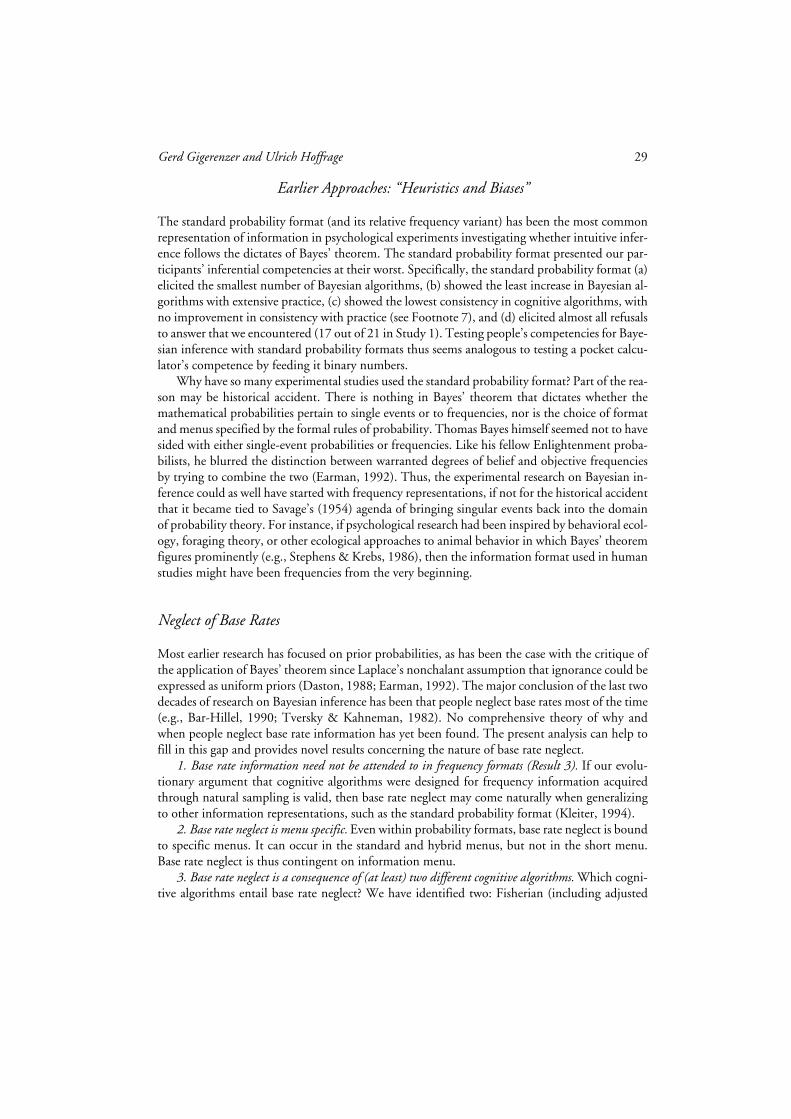
Gerd Gigerenzer and Ulrich Hoffrage 29
Earlier Approaches: “Heuristics and Biases”
The standard probability format (and its relative frequency variant) has been the most commonrepresentation of information in psychological experiments investigating whether intuitive infer-ence follows the dictates of Bayes’ theorem. The standard probability format presented our par-ticipants’ inferential competencies at their worst. Specifically, the standard probability format (a)elicited the smallest number of Bayesian algorithms, (b) showed the least increase in Bayesian al-gorithms with extensive practice, (c) showed the lowest consistency in cognitive algorithms, withno improvement in consistency with practice (see Footnote 7), and (d) elicited almost all refusalsto answer that we encountered (17 out of 21 in Study 1). Testing people’s competencies for Baye-sian inference with standard probability formats thus seems analogous to testing a pocket calcu-lator’s competence by feeding it binary numbers.
Why have so many experimental studies used the standard probability format? Part of the rea-son may be historical accident. There is nothing in Bayes’ theorem that dictates whether themathematical probabilities pertain to single events or to frequencies, nor is the choice of formatand menus specified by the formal rules of probability. Thomas Bayes himself seemed not to havesided with either single-event probabilities or frequencies. Like his fellow Enlightenment proba-bilists, he blurred the distinction between warranted degrees of belief and objective frequenciesby trying to combine the two (Earman, 1992). Thus, the experimental research on Bayesian in-ference could as well have started with frequency representations, if not for the historical accidentthat it became tied to Savage’s (1954) agenda of bringing singular events back into the domainof probability theory. For instance, if psychological research had been inspired by behavioral ecol-ogy, foraging theory, or other ecological approaches to animal behavior in which Bayes’ theoremfigures prominently (e.g., Stephens & Krebs, 1986), then the information format used in humanstudies might have been frequencies from the very beginning.
Neglect of Base Rates
Most earlier research has focused on prior probabilities, as has been the case with the critique ofthe application of Bayes’ theorem since Laplace’s nonchalant assumption that ignorance could beexpressed as uniform priors (Daston, 1988; Earman, 1992). The major conclusion of the last twodecades of research on Bayesian inference has been that people neglect base rates most of the time(e.g., Bar-Hillel, 1990; Tversky & Kahneman, 1982). No comprehensive theory of why andwhen people neglect base rate information has yet been found. The present analysis can help tofill in this gap and provides novel results concerning the nature of base rate neglect.
1. Base rate information need not be attended to in frequency formats (Result 3). If our evolu-tionary argument that cognitive algorithms were designed for frequency information acquiredthrough natural sampling is valid, then base rate neglect may come naturally when generalizingto other information representations, such as the standard probability format (Kleiter, 1994).
2. Base rate neglect is menu specific. Even within probability formats, base rate neglect is boundto specific menus. It can occur in the standard and hybrid menus, but not in the short menu.Base rate neglect is thus contingent on information menu.
3. Base rate neglect is a consequence of (at least) two different cognitive algorithms. Which cogni-tive algorithms entail base rate neglect? We have identified two: Fisherian (including adjusted
30 How to Improve Bayesian Reasoning
Fisherian) and likelihood subtraction (including its shortcut version, false alarm complement).Neither of these can be elicited in the short menu.
4. Process analysis is indispensable in establishing base rate neglect. This last point is methodolog-ical. Cognitive algorithms having in common the neglect of base rate information can neverthe-less entail different probability judgments. Thus, no single probability judgment can be deducedfrom base rate neglect per se. The same holds for the inverse inference, from probability judg-ment to base rate neglect. A particular probability judgment can be produced by various algo-rithms, including ones that do and do not use base rates (see Birnbaum’s, 1983, insightful anal-ysis of the cab problem). Thus, base rate neglect cannot safely be inferred from a particular prob-ability judgment, that is, from mere outcome analysis, without being double-checked by processanalysis, such as “write aloud” protocols. Working through several thousand individual proto-cols, we observed many cases where probabilities of similar magnitude were computed by differ-ent cognitive algorithms. However, almost all previous work has relied on outcome analysis only.
Representativeness Heuristic
Tversky and Kahneman’s (1974, 1982) “representativeness heuristic” has so far provided themost widely used explanation for base rate neglect in terms of a cognitive process. Judgment byrepresentativeness means that the probability p(H|D) is inferred from the similarity between Dand H. However, how this similarity is computed and how the inference from the similarity to anumerical probability is made have not been clarified since the notion was first proposed; “rep-resentativeness” is consequently still vague and undefined (Shanteau, 1989). Furthermore, it isnot applicable to most of the problems in Studies 1 and 2, including all medical problems andthe cab problem (e.g., it makes little sense to ask how representative a mother’s German measlesare of a child’s rubella syndrome). We suggest defining the notion of representativeness by thestatistical concept of the likelihood p(D|H), a proposal made by Gigerenzer and Murray (1987,pp. 153–155). We thereby treat the representativeness heuristic as a special case of the Fisherianalgorithm—namely, when the likelihood is interpreted as a degree of similarity between D andH. If one accepts this proposal, two interesting implications follow:
1. Frequency formats suppress inference by “representativeness.” We observed that use of theFisherian algorithm decreased from 99 cases in the probability format to 55 cases in the frequencyformat (including the adjusted variant, see Table 3). This format dependency is a striking empir-ical result. Nothing prevented our participants from picking “d out of h” in the frequency formatas often as picking p(D|H) in the probability format. The decrease occurred generally in all prob-lems, whether p(D|H) could be interpreted as a similarity relation or not.
2. The “representativeness heuristic” is menu specific. Inferences by “representativeness” can beelicited by the standard menu, but not by the short menu (Tables 3 and 4). Thus, when infor-mation is acquired by natural sampling, representativeness should play no role.
If we take these two implications together, then we arrive at the result that the representative-ness heuristic is most likely to be elicited when information is represented in the standard prob-ability format. This result provides a partial answer to the unresolved question of what conditionsfavor particular heuristics (Brown & Siegler, 1993).
Gerd Gigerenzer and Ulrich Hoffrage 31
Pseudodiagnosticity
Most of the research on Bayesian inference has focused on the neglect of base rates, but a fewstudies have investigated the use or neglect of p(D|–H) in Bayesian inference. The phenomenonof people ignoring p(D|–H) has been termed pseudodiagnosticity (Doherty & Mynatt, 1990;Fischhoff & Beyth-Marom, 1983; Ofir, 1988). The term stems from an information selectiontask in which participants are presented with both p(D|H) and p(D|–H) but tend to use only oneof the two likelihoods, usually p(D|H). Our analysis revealed that the false alarm rate was aboutas often neglected as the base rate. In Studies 1 and 2, the false alarm rate was neglected in 31%and 33% of cases, the base rate in 32% and 36%, respectively (these are conservative estimatesbecause the less frequent algorithms are not counted). We were able to identify cognitive algo-rithms underlying this phenomenon: joint occurrence, Fisherian, and base rate only.
Do Frequency Formats Influence Statistical Reasoning Beyond Bayesian Inference?
It is interesting that most so-called biases and fallacies in probabilistic and statistical reasoning,such as base rate neglect, have been demonstrated using problems with probability formats. Canfrequency formats affect other “cognitive illusions”? The evidence suggests so (see Tversky &Kahneman, 1974). Gigerenzer et al. (1991) showed that the “overconfidence bias” (e.g., Lichten-stein et al., 1982) disappeared when participants estimated frequencies instead of single-eventprobabilities (see also May, 1987; Sniezek & Buckley, 1993). This seems to be the only case asidefrom the present analysis of Bayesian inference where a cognitive algorithm is proposed, namelyby the theory of probabilistic mental models (Gigerenzer, 1993a; Gigerenzer et al., 1991), to ex-plain why and how format affects inferences. The theory additionally specifies conditions inwhich frequency judgments can be made less realistic than probability judgments.
Fiedler (1988) and Hertwig and Gigerenzer (1995) showed that the “conjunction fallacy”(Tversky & Kahneman, 1983) in the Linda problem and similar problems largely disappearedwhen questions were changed from probability to frequency formats; the proportion of conjunc-tion rule violations dropped from more than 80% to about 10% to 20% (see also Reeves & Lock-hart, 1993; Tversky & Kahneman, 1983). As with the “overconfidence bias,” this effect of fre-quency format is stronger and more reliable than those of all earlier so-called debiasing methods(as summarized by Fischhoff, 1982).
Koehler, Gibbs, and Hogarth (1994) reported that the “illusion of control” (Langer, 1975)is reduced when the single-event format is replaced by a frequency format—when participantsjudge a series of events rather than a single event. Teigen (1974) reported that overestimation ofprobabilities (e.g., What is the probability that a randomly chosen female student at the Univer-sity of Bergen is above 160 cm tall?) changed into more realistic estimates when participants weregiven the opportunity to estimate frequencies (e.g., If we measure 500 female students, howmany of them will be above 160 cm tall?). Keren and Wagenaar (1987) observed that the “cer-tainty effect” and the “possibility effect,” two violations of utility theory, occurred less often whensingle gambles were replaced by repeated gambles (see also Keren, 1991; Montgomery & Adel-bratt, 1982). For a general discussion of these results see Ayton and Wright (1994), Gigerenzer(1991a, 1991b, 1993a, 1994), and Lopes (1981).
32 How to Improve Bayesian Reasoning
These converging results do have implications for how to understand so-called cognitive illu-sions. Were cognitive illusions due to the mind’s inherent inability to reason statistically, or ifthey were simply the result of wishful thinking or other motivational deficits, then a frequencyformat should make no difference. The evidence so far, however, suggests that frequency formatcan make quite a difference.
Some Practical Consequences
Cognitive algorithms, Bayesian or otherwise, cannot be divorced from the information on whichthey operate and how that information is represented. This striking result can be made useful forteaching statistical reasoning and for human engineering in general (von Winterfeldt & Edwards,1986). The problems used in our studies, such as pregnancy tests, mammograms, and HIV tests,exemplify situations where Bayesian inference can help people to grasp the risks and uncertaintiesof a modern, technological world. However, the teaching of statistical reasoning is still a field ne-glected in high-school mathematics education (Shaughnessy, 1992), and instruction in Bayesianinference seems to be almost nonexistent. Up until now, only a few studies have attempted toteach Bayesian inference, mainly by outcome feedback, and with little or no success (Lindeman,van den Brink, & Hoogstraten, 1988; Peterson, DuCharme, & Edwards, 1968; Schaefer, 1976).
The present framework suggests an effective way to teach Bayesian inference and statisticalreasoning generally. The lesson of our studies is to teach representations instead of rules, that is,to teach people how to translate probabilities into frequency representations rather than how toinsert probabilities into Equation 1. In light of our results concerning how Bayesian inference canbe improved without any instruction, tutoring systems that enhance the idea of frequency repre-sentations with instruction, explanation, and visual aids hold out the promise of still greater suc-cess. Frequency representations can help people “see” the answer, appealing to a “sort of instinct”at which Laplace and the Enlightenment probabilists hinted.
References
Ajzen, I. (1977). Intuitive theories of events and the effects of base-rate information on predictions. Journal of Per-sonality and Social Psychology, 35, 303–314.
Allais, M. (1953). Le comportement de l’homme rationnel devant le risque: Critique des postulats et axiomes del’Ecole Américaine [The behavior of rational man with respect to risk: A criticism of the postulates and axiomsof the American school]. Economctrica, 21, 503–546.
Ayton, P., & Wright, G. (1994). Subjective probability: What should we believe? In G. Wright & P. Ayton (Eds.),Subjective probability (pp. 163–184). New York: Wiley.
Bar-Hillel, M. (1980). The base-rate fallacy in probability judgments. Acta Psychologica, 44, 211–233.Bar-Hillel, M. (1990). Back to base rates. In R. M. Hogarth (Ed.), Insights in decision making (pp. 309–330).
Chicago: University of Chicago Press.Barsalou, L. W., & Ross, B. H. (1986). The role of automatic and strategic processing in sensitivity to superordi-
nate and property frequency. Journal of Experimental Psychology: Learning, Memory, and Cognition, 12, 116–134.
Bayes, T. (1763). An essay towards solving a problem in the doctrine of chances. Philosophical Transactions of theRoyal Society of London, 53, 370–418.
Birnbaum, M. H. (1983). Base rates in Bayesian inference: Signal detection analysis of the cab problem. AmericanJournal of Psychology, 96, 85–94.
Boole, G. (1958). An investigation of the laws of thought. New York: Dover. (Original work published 1854)
Gerd Gigerenzer and Ulrich Hoffrage 33
Borgida, E., & Brekke, N. (1981). The base-rate fallacy in attribution and prediction. In J. H. Harvey, W. J. Ickes,& R. F. Kidd (Eds.), New directions in attribution research (pp. 66–95). Hillsdale, NJ: Erlbaum.
Brown, N. R., & Siegler, R. S. (1993). Metrics and mappings: A framework for understanding real-world quan-titative estimation. Psychological Review, 100, 511–534.
Brunswik, E. (1939). Probability as a determiner of rat behavior. Journal of Experimental Psychology, 25, 175–197.Brunswik, E. (1955). Representative design and probabilistic theory in a functional psychology. Psychological Re-
view, 62, 193–217.Casscells, W., Schoenberger, A., & Grayboys, T. (1978). Interpretation by physicians of clinical laboratory results.
New England Journal of Medicine, 299, 999–1000.Christensen-Szalanski, J. J. J., & Beach, L. R. (1982). Experience and the base-rate fallacy. Organizational Behav-
ior and Human Performance, 29, 270–278.Cohen, J. (1977). Statistical power analysis for the behavioral sciences (2nd ed.). New York: Academic Press.Cohen, L. J. (1986). The dialogue of reason. Oxford, England: Clarendon Press.Cosmides, L., & Tooby, J. (in press). Are humans good intuitive statisticians after all? Rethinking some conclu-
sions from the literature on judgment under uncertainty. Cognition.Daston, L. J. (1981). Mathematics and the moral sciences: The rise and fall of the probability of judgments, 1785–
1840. In H. N. Jahnke & M. Otte (Eds.), Epistemological and social problems of the sciences in the early nine-teenth century (pp. 287–309). Dordrecht, The Netherlands: D. Reidel.
Daston, L. J. (1988). Classical probability in the Enlightenment. Princeton, NJ: Princeton University Press.Doherty, M. E., & Mynatt, C. R. (1990). Inattention to p(H) and to p(D|–H): A converging operation. Acta
Psychologica, 75, 1–11.Earman, J. (1992). Bayes or bust? A critical examination of Bayesian confirmation theory. Cambridge, MA: MIT
Press.Eddy, D. M. (1982). Probabilistic reasoning in clinical medicine: Problems and opportunities. In D. Kahneman,
P. Slovic, & A. Tversky (Eds.), Judgment under uncertainty: Heuristics and biases (pp. 249–267). Cambridge,England: Cambridge University Press.
Edwards, W. (1968). Conservatism in human information processing. In B. Kleinmuntz (Ed.), Formal represen-tation of human judgment (pp. 17–52). New York: Wiley.
Edwards, W., & von Winterfeldt, D. (1986). On cognitive illusions and their implications. In H. R. Arkes & K.R. Hammond (Eds.), Judgment and decision making. Cambridge, England: Cambridge University Press.
Ericsson, K. A., & Simon, H. A. (1984). Protocol analysis: Verbal reports as data. Cambridge, MA: MIT Press.Feynman, R. (1967). The character of physical law. Cambridge, MA: MIT Press.Fiedler, K. (1988). The dependence of the conjunction fallacy on subtle linguistic factors. Psychological Research,
50, 123–129. Fischhoff, B. (1982). Debiasing. In D. Kahneman, P. Slovic, & A. Tversky (Eds.), Judgment under uncertainty:
Heuristics and biases (pp. 422–444). Cambridge, England: Cambridge University Press.Fischhoff, B., & Beyth-Marom, R. (1983). Hypothesis evaluation from a Bayesian perspective. Psychological Re-
view, 90, 239–260.Fisher, R. A. (1955). Statistical methods and scientific induction. Journal of the Royal Statistical Society, Series B,
17, 69–78.Gallistel, C. R. (1990). The organization of learning. Cambridge, MA: MIT Press.Gavanski, I., & Hui, C. (1992). Natural sample spaces and uncertain belief. Journal of Personality and Social Psy-
chology, 63, 766–780.Gigerenzer, G. (1991a). From tools to theories: A heuristic of discovery in cognitive psychology. Psychological Rex-
iew, 98, 254–267.Gigerenzer, G. (1991b). How to make cognitive illusions disappear. Beyond “heuristics and biases.” In W.
Stroebe & M. Hewstone (Eds.), European Review of Social Psychology, 2, 83–115.Gigerenzer, G. (1993a). The bounded rationality of probabilistic mental models. In K. I. Manktelow & D. E.
Over (Eds.), Rationality: Psychological and philosophical perspectives (pp. 284–313). London: Routledge.Gigerenzer, G. (1993b). The superego, the ego, and the id in statistical reasoning. In G. Keren & C. Lewis (Eds.),
A handbook for data analysis in the behavioral sciences: Methodological issues (pp. 313–339). Hillsdale, NJ:Erlbaum.
Gigerenzer, G. (1994). Why the distinction between single-event probabilities and frequencies is relevant for psy-chology (and vice versa). In G. Wright & P. Ayton (Eds.), Subjective probability (pp. 129–162). New York:Wiley.
Gigerenzer, G., & Goldstein, D. G. (1995). Reasoning the fast and frugal way: Models of bounded rationality. Manu-script submitted for publication.
Gigerenzer, G., Hell, W., & Blank, H. (1988). Presentation and content: The use of base rates as a continuousvariable. Journal of Experimental Psychology: Human Perception and Performance, 14, 513–525.
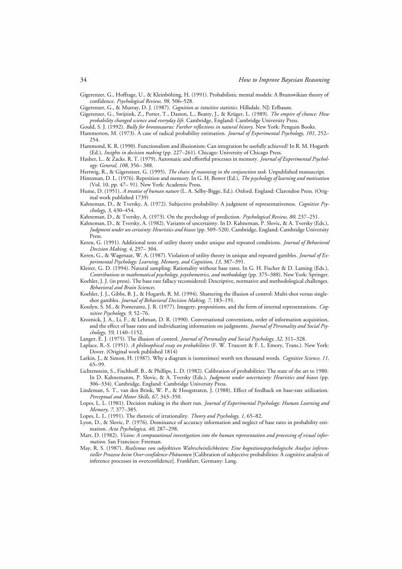
34 How to Improve Bayesian Reasoning
Gigerenzer, G., Hoffrage, U., & Kleinbölting, H. (1991). Probabilistic mental models: A Brunswikian theory ofconfidence. Psychological Review, 98, 506–528.
Gigerenzer, G., & Murray, D. J. (1987). Cognition as intuitive statistics. Hillsdale. NJ: Erlbaum. Gigerenzer, G., Swijtink, Z., Porter, T., Daston, L., Beatty, J., & Krüger, L. (1989). The empire of chance: How
probability changed science and everyday life. Cambridge, England: Cambridge University Press.Gould, S. J. (1992). Bully for brontosaurus: Further reflections in natural history. New York: Penguin Books.Hammerton, M. (1973). A case of radical probability estimation. Journal of Experimental Psychology, 101, 252–
254.Hammond, K. R. (1990). Functionalism and illusionism: Can integration be usefully achieved? In R. M. Hogarth
(Ed.), Insights in decision making (pp. 227–261). Chicago: University of Chicago Press.Hasher, L.. & Zacks. R. T. (1979). Automatic and effortful processes in memory. Journal of Experimental Psychol-
ogy: General, 108, 356– 388.Hertwig, R., & Gigerenzer, G. (1995). The chain of reasoning in the conjunction task. Unpublished manuscript.Hintzman, D. L. (1976). Repetition and memory. In G. H. Bower (Ed.), The psychology of learning and motivation
(Vol. 10, pp. 47– 91). New York: Academic Press.Hume, D. (1951). A treatise of human nature (L. A. Selby-Bigge, Ed.). Oxford. England: Clarendon Press. (Orig-
inal work published 1739)Kahneman, D., & Tversky, A. (1972). Subjective probability: A judgment of representativeness. Cognitive Psy-
chology, 3, 430–454.Kahneman, D., & Tversky, A. (1973). On the psychology of prediction. Psychological Review, 80, 237–251.Kahneman, D., & Tversky, A. (1982). Variants of uncertainty. In D. Kahneman, P. Slovic, & A. Tversky (Eds.),
Judgment under un certainty: Heuristics and biases (pp. 509–520). Cambridge, England: Cambridge UniversityPress.
Keren, G. (1991). Additional tests of utility theory under unique and repeated conditions. Journal of BehavioralDecision Making, 4, 297– 304.
Keren, G., & Wagenaar, W. A. (1987). Violation of utility theory in unique and repeated gambles. Journal of Ex-perimental Psychology: Learning, Memory, and Cognition, 13, 387–391.
Kleiter, G. D. (1994). Natural sampling: Rationality without base rates. In G. H. Fischer & D. Laming (Eds.),Contributions to mathematical psychology, psyxhometrics, and methodology (pp. 375–388). New York: Springer.
Koehler, J. J. (in press). The base rate fallacy reconsidered: Descriptive, normative and methodological challenges.Behavioral and Brain Sciences.
Koehler, J. J., Gibbs, B. J., & Hogarth, R. M. (1994). Shattering the illusion of control: Multi-shot versus single-shot gambles. Journal of Behavioral Decision Making, 7, 183–191.
Kosslyn, S. M., & Pomerantz, J. R. (1977). Imagery, propositions, and the form of internal representations. Cog-nitive Psychology, 9, 52–76.
Kroznick, J. A., Li, F., & Lehman, D. R. (1990). Conversational conventions, order of information acquisition,and the effect of base rates and individuating information on judgments. Journal of Personality and Social Psy-chology, 59, 1140–1152.
Langer, E. J. (1975). The illusion of control. Journal of Personality and Social Psychology, 32, 311–328.Laplace, R.-S. (1951). A philosophical essay on probabilities (F. W. Truscott & F. L. Emory, Trans.). New York:
Dover. (Original work published 1814)Larkin, J., & Simon, H. (1987). Why a diagram is (sometimes) worth ten thousand words. Cognitive Science, 11,
65–99.Lichtenstein, S., Fischhoff. B., & Phillips, L. D. (1982). Calibration of probabilities: The state of the art to 1980.
In D. Kahnemanm, P. Slovic, & A. Tversky (Eds.), Judgment under uncertainty: Heuristics and biases (pp.306–334). Cambridge, England: Cambridge University Press.
Lindeman, S. T., van den Brink, W. P., & Hoogstraten, J. (1988). Effect of feedback on base-rate utilization.Perceptual and Motor Skills, 67, 343–350.
Lopes, L. L. (1981). Decision making in the short run. Journal of Experimental Psychology: Human Learning andMemory, 7, 377–385.
Lopes, L. L. (1991). The rhetoric of irrationality. Theory and Psychology, 1, 65–82.Lyon, D., & Slovic, P. (1976). Dominance of accuracy information and neglect of base rates in probability esti-
mation. Acta Psychologica, 40, 287–298.Marr, D. (1982). Vision: A computational investigation into the human representation and processing of visual infor-
mation. San Francisco: Freeman.May, R. S. (1987). Realismus von subjektiven Wahrscheinlichkeiten: Eine kognitionspsychologische Analyse inferen-
tieller Prozesse beim Over-confidence-Phänomen [Calibration of subjective probabilities: A cognitive analysis ofinference processes in overconfidence]. Frankfurt, Germany: Lang.
Gerd Gigerenzer and Ulrich Hoffrage 35
McKenzie, C. R. (1994). The accuracy of intuitive judgment strategies: Covariation assessment and Bayesian in-ference. Cognitive Psychology, 26, 209–239.
Medin, D. L., Wattenmaker, W. D., & Michalski, R. S. (1987). Constraints and preferences in inductive learn-ing: An experimental study of human and machine performance. Cognitive Science, 11, 299– 339.
Montgomery, H., & Adelbratt, T. (1982). Gambling decisions and information about expected value. Organiza-tional Behavior and Human Performance, 29, 39–57.
Nisbett, R. E., & Wilson, T. D. (1977). Telling more than we can know: Verbal reports on mental processes.Psychological Review, 84, 231– 259.
Oakes, M. (1986). Statistical inference: A commentary for the social and behavioral sciences. New York: Wiley.Ofir, C. (1988). Pseudodiagnosticity in judgment under uncertainty. Organizational Behavior and Human Deci-
sion Processes, 42, 343–363.Peterson, C. R., DuCharme, W. M., & Edwards, W. (1968). Sampling distributions and probability revision.
Journal of Experimental Psychology, 76, 236–243.Phillips, L. D., & Edwards, W. (1966). Conservatism in a simple probability model inference task. Journal of Ex-
perimental Psychology, 72, 346–354.Piaget, J., & Inhelder, B. (1975). The origin of the idea of chance in children. New York: Norton. (Original work
published 1951)Pylyshyn, Z. W. (1973). What the mind’s eye tells the mind’s brain: A critique of mental imagery. Psychological
Bulletin, 80, 1–24.Real, L. A. (1991, August). Animal choice behavior and the evolution of cognitive architecture. Science, 253, 980–986.Real, L. A., & Caraco, T. (1986). Risk and foraging in stochastic environments: Theory and evidence. Annual
Review of Ecology and Systematics, 77, 371–390.Reeves, T., & Lockhart, R. (1993). Distributional versus singular approaches to probability and errors in proba-
bilistic reasoning. Journal of Experimental Psychology: General, 122, 207–226.Rouanet, H. (1961). Études de décisions expérimentales et calcul de probabilités. [Studies of experimental deci-
sion making and the probability calculus] In Colloques internationaux du centre national de la recherche scien-tifique (pp. 33–43). Paris: Éditions du Centre National de la Recherche Scientifique.
Sahlin, N. (1993). On higher order beliefs. In J. Dubucs (Ed.), Philosophy of probability (pp. 13–34). Dordrecht,The Netherlands: Kluwer Academic.
Savage, L. J. (1954). The foundations of statistics. New York: Wiley.Schaefer, R. E. (1976). The evaluation of individual and aggregated subjective probability distributions. Organi-
zational Behavior and Human Performance, 17, 199–210.Scholz, R. W. (1987). Cognitive strategies in stochastic thinking. Dordrecht, The Netherlands: D. Reidel. Schum, D. A. (1994). The evidential foundations of probabilistic reasoning. New York: Wiley.Sedlmeier, P., Hertwig, R., & Gigerenzer, G. (1995). Is “R ” more likely in the first or second position? Availability,
letter class, and neural network models. Manuscript submitted for publication.Shanks, D. (1991). A connectionist account of base-rate biases in categorization. Connection Science, 5 (2), 143–162.Shanteau, J. (1989). Cognitive heuristics and biases in behavioral auditing: Review, comments and observations.
Accounting Organizations and Society, 74 (1/2), 165–177.Shaughnessy, J. M. (1992). Research on probability and statistics: Reflections and directions. In D. A. Grouws
(Ed.), Handbook of research on mathematical teaching and learning (pp. 465–499). New York: Macmillan.Simon, H. A. (1956). Rational choice and the structure of the environment. Psychological Review, 63, 129–138.Sniezek, J. A., & Buckley, T. (1993). Decision errors made by individuals and groups. In N. J. Castellan (Ed.),
Individual and group decision making. Hillsdale, NJ: Erlbaum.Stephens, D. W., & Krebs, J. R. (1986). Foraging theory. Princeton, NJ: Princeton University Press.Stigler, J. W. (1984). The effect of abacus training on Chinese children’s mental calculation. Cognitive Psychology,
16, 145–176.Teigen, K. H. (1974). Overestimation of subjective probabilities. Scandinavian Journal of Psychology, 15, 56–62.Tversky, A., & Kahneman, D. (1974, September). Judgment under uncertainty: Heuristics and biases. Science,
185, 1124–1131.Tversky, A., & Kahneman, D. (1982). Evidential impact of base rates. In D. Kahneman, P. Slovic, & A. Tversky
(Eds.), Judgment under uncertainty: Heuristics and biases (pp. 153–160). Cambridge, England: CambridgeUniversity Press.
Tversky, A., & Kahneman, D. (1983). Extensional versus intuitive reasoning: The conjunction fallacy in proba-bility judgment. Psychological Review, 90, 293–315.
von Winterfeldt, D., & Edwards, W. (1986). Decision analysis and behavioral research. Cambridge, England: Cam-bridge University Press.
Wallsten, T. S. (1983). The theoretical status of judgmental heuristics. In R. W. Scholz (Ed.), Decision makingunder uncertainty (pp. 21–39). Amsterdam: Elsevier (North-Holland).
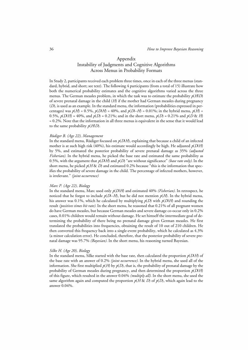
36 How to Improve Bayesian Reasoning
AppendixInstability of Judgments and Cognitive Algorithms
Across Menus in Probability Formats
In Study 2, participants received each problem three times, once in each of the three menus (stan-dard, hybrid, and short; see text). The following 4 participants (from a total of 15) illustrate howboth the numerical probability estimates and the cognitive algorithms varied across the threemenus. The German measles problem, in which the task was to estimate the probability p(H|D)of severe prenatal damage in the child (H) if the mother had German measles during pregnancy(D), is used as an example. In the standard menu, the information (probabilities expressed in per-centages) was p(H) = 0.5%, p(D|H) = 40%, and p(D|–H) = 0.01%; in the hybrid menu, p(H) =0.5%, p(D|H) = 40%, and p(D) = 0.21%; and in the short menu, p(D) = 0.21% and p(D & H)= 0.2%. Note that the information in all three menus is equivalent in the sense that it would leadto the same probability p(H|D).
Rüdiger B. (Age 22), ManagementIn the standard menu, Rüdiger focused on p(D|H), explaining that because a child of an infectedmother is at such high risk (40%), his estimate would accordingly be high. He adjusted p(D|H)by 5%, and estimated the posterior probability of severe prenatal damage as 35% (adjustedFisherian). In the hybrid menu, he picked the base rate and estimated the same probability as0.5%, with the argument that p(D|H) and p(D) “are without significance” (base rate only). In theshort menu, he picked p(H & D) and estimated 0.2% because “this is the information that spec-ifies the probability of severe damage in the child. The percentage of infected mothers, however,is irrelevant.” (joint occurrence)
Marc P. (Age 22), BiologyIn the standard menu, Marc used only p(D|H) and estimated 40% (Fisherian). In retrospect, henoticed that he forgot to include p(D|–H), but he did not mention p(H). In the hybrid menu,his answer was 0.1%, which he calculated by multiplying p(D) with p(D|H) and rounding theresult (positives times hit rate). In the short menu, he reasoned that 0.21% of all pregnant womendo have German measles, but because German measles and severe damage co-occur only in 0.2%cases, 0.01% children would remain without damage. He set himself the intermediate goal of de-termining the probability of there being no prenatal damage given German measles. He firsttranslated the probabilities into frequencies, obtaining the result of 10 out of 210 children. Hethen converted this frequency back into a single-event probability, which he calculated as 4.3%(a minor calculation error). He concluded, therefore, that the posterior probability of severe pre-natal damage was 95.7% (Bayesian). In the short menu, his reasoning turned Bayesian.
Silke H. (Age 20), BiologyIn the standard menu, Silke started with the base rate, then calculated the proportion p(D|H) ofthe base rate with an answer of 0.2% (joint occurrence). In the hybrid menu, she used all of theinformation. She first multiplied p(H) by p(D), that is, the probability of prenatal damage by theprobability of German measles during pregnancy, and then determined the proportion p(D|H)of this figure, which resulted in the answer 0.04% (multiply all). In the short menu, she used thesame algorithm again and computed the proportion p(H & D) of p(D), which again lead to theanswer 0.04%.

Gerd Gigerenzer and Ulrich Hoffrage 37
Oliver G. (Age 22), German LiteratureIn the standard menu, Oliver stated that the “correlation between not having damage and nev-ertheless having measles,” as he paraphrased p(D|–H), was the only relevant information. He cal-culated 1 – p(D|–H) = 99.99% and rounded to 100%, which was his estimate (false alarm com-plement). In the hybrid menu, he concluded that the only relevant information was the base rateof severe prenatal damage, and his estimate consequently dropped to 0.5% (base rate only). In theshort menu, he determined the proportion of severe damage and measles in all cases with Germanmeasles, which led him to the Bayesian answer of 95.3%.