How To Be Smooth: Automated Smoothing in PoliticalScience

Luke Keele2140 Derby Hall

150 North Oval MallOhio State UniversityColumbus, OH 43210

March 9, 2006

Abstract

Smoothing is an important statistical tool in applied analysis of political data. Smootherscan be use to incorporate nonlinearity, deal with duration dependence, and diagnose residualplots. But smoothers invariably require the analyst to make choices about the amount ofsmoothing to apply and the criteria for this choice amounts to visual examination. Suchvisual methods can lead to seemingly arbitrary selection of smoothing parameters. I arguethat instead of using a visual method for the selection of smoothing parameters, analystsshould use automated methods where the level of smoothing is estimated from the data. Ioutline why such methods are preferable and then demonstrate with both simulated data andin empirical settings how automatic smoothing is superior to visual selection of smoothingparameters.

Methods of smoothing the statistical relationship between two variables have gained in-

creased currency in political science. Smoothers, often referred to as scatterplot smoothers

or nonparametric regression, have a variety of uses. They can be used to incorporate nonlin-

earity into parametric models (Beck and Jackman 1998; Keele 2006). They can be used to

smooth plots of hazard functions (Box-Steffensmeier and Jones 2004). They are also a key

technique for the estimation of binary time-series cross sectional datasets (Beck, Katz and

Tucker 1998). They can also be an important diagnostic tool for linear model residual plots

(Fox 1997).

While smoothers are readily available in a variety of statistical software packages, their

use isn’t without complications. First, there are a bewildering array of different smoothers.

For example, there are at least four different types of spline smoothers alone. Moreover,

while smoothers replace strong linearity assumptions, analysts who use smoothers have to

1

make choices about bandwidth and smoothing parameters, knot numbers and placement,

and basis functions depending on the type of smoother. These choices all have consequences

for how smooth the fit between x and y is. Evaluation of these choices is typically done with

a visual method of trial and error with only theory as a guide for how smooth a process

may be. Some authors have even described the choices revolving around the smoothers as

“controversial” (Box-Steffensmeier and Jones 2004). This has led some analysts to see the

use of smoothers as more akin to art than science.

I argue that most often theories in social science are silent about the smoothness of

the process making it a poor guide for the selection of modeling parameters. Moreover, in

many situations where smoothers are applied we cannot reasonably expect analysts to have

theories. For example, the smoothing of time terms or using smoothers for diagnostic plots

are situations where there will never be any theory to guide the analyst. Instead, I advocate

the use of smoothing techniques where the amount of smoothness imposed is estimated from

the data. Such methods often provide a better fit to the data and more importantly produce

confidence bands that better reflect our uncertainty about the level of smoothness.

What follows, here, is first an overview of the basic types of smoothers available. More

importantly I clarify the choices required in the use of each. I, then, introduce automatic

smoothing techniques focusing on smoothing splines where the knot placement and selection is

automatic and the smoothing parameter is estimated via either cross validation or restricted

maximum likelihood estimation. I, then, conduct a comparative analysis of smoothers to

demonstrate how smoothing splines with automatic smoothing outperforms other techniques.

I finish with some empirical examples to show how smoothing splines might be used in

practice.

1 So Many Smoothers, So Many Choices

Smoothers fall into three basic classes: kernel smoothers, local polynomial regression, and

splines. I restrict my attention, here to local polynomial regression and, in particular, splines.

Kernel smoothers get very little use in political science and in other fields since splines and

local polynomial regression incorporate many of the desirable properties of kernel smoothers

2

but offer other advantages.

In local polynomial regression, the smoother works by performing a weighted polynomial

regression for some small segment of the data. For an excellent introduction to local polyno-

mial regression see Fox (2000). Among local polynomial smoothers one can use loess, lowess,

and local likelihood.

Splines are piecewise polynomial functions that are constrained to join at points called

knots. In their simplest form, splines are just regression models with restricted dummy

regressors. They force the regression line to change direction at some point along the range

of x. Separate regression lines are fit within the regions between the knots. The term “spline”

come from a tool used by draftsman to draw curves. There are a variety of splines including

regression splines, cubic splines (often referred to as cubic B-splines), natural splines, and

smoothing splines. To make matters worse smoothing splines are often referred to as p-splines,

penalized splines, or pseudosplines all of which are, for the most part, interchangeable terms

for a smoothing spline.

When using local polynomial smoothers, an analyst must make three choices: the degree

of the polynomial, the bandwidth or span, and the kernel. However, two of these choices

are almost always of little import. The degree of the polynomial is almost always quadratic

and occasionally cubic. Higher degree polynomials have more coefficients resulting in higher

variability which is undesirable (Fox 2000). In fact most software won’t allow the analyst

to choose anything more than a second degree polynomial.1 While analysts can also choose

among a variety of kernels, which are used to provide weights for the local regression model

almost all local regression smoothers use a tri-cube kernel. In practice, different kernels

typically make little difference.

The important choice when using a local polynomial smoother is that of bandwidth

or span. The bandwidth controls how much data is used for each local regression, which

directly translate into how smooth the fit is between x and y. As the bandwidth increases,

the smoother the nonparametric fit between x and y is, and for very small bandwidths the

smoother will interpolate between data points giving a very rough fit between x and y. It

is often convenient to specify the degree of smoothing as the proportion of the observations

1For example, the lowess command in both Stata and R will not let the user adjust the degree of polynomialused.

3

that will be included in the window. This fraction of the data is called the span, s, of a local-

regression smoother and it is an exact function of the bandwidth. The choice of bandwidth or

span reflects a choice between bias and variance. Smoother fits tend to have higher amounts

of bias but little variance, while rougher fits will exhibit little bias but large amounts of

variability. See Beck and Jackman (1998) or Fox (2000) demonstrations of this tradeoff. It

would seem that the amount of smoothing to apply then would be the solution to a mean

squared error problem. We will exploit this equivalence later.

The typical method for selection of the span or bandwidth parameter is one of visual trial

and error. We want the smallest span that provides a smooth fit that is we want the span

that minimizes both the bias and variability of the smoothed fit. A typical starting point

is a span of 0.5 which implies that 50% of the data will be included in the local fit. If the

fitted smoother looks too rough the span is increased, if it looks smooth, we see if it can be

decreased without making the fit too rough. 2

While local polynomial smoothers are very useful for scatterplot smoothing and other

basic uses of smoothers, the focus on most of the research on smoothing in statistics has been

on splines. Splines more readily lend themselves to incorporation into parametric models in

the form of generalized additive models (GAMs), are more flexible and have better analytic

properties (Wood 2006). The most recent texts on smoothing and semiparametic estimation

focus almost exclusively on splines with local polynomial regression being mentioned only in

passing (Ruppert, Wand and Carroll 2003; Wood 2006).

2 Splines: How Many Knots and Where Do I Tie

Them?

As I mentioned before, splines are piecewise polynomial functions that are constrained to

join at points called knots. As I mentioned before there are a variety of splines but most

of these names differ due to advances in spline fitting techniques. While the choice of the

polynomial degree and basis functions used to matter, they are of little consequence now. In

2There are automatic methods for selection of the bandwidth parameter but I don’t discuss them since unlikewith smoothing splines the confidence intervals for these automatic routines do not reflect uncertainty in thebandwidth estimates.

4

applied use, most analysts use natural cubic B-splines. Cubic splines are made to be smooth

at the knots by forcing the first and second derivatives of the function to agree at the knots.

Natural cubic splines constrain the pattern to be linear before the first knot and after the

last knot by adding a knot at each boundary. This requirement avoids wild behavior near

the extremes of the data. B-basis functions are used for numerical stability (Ruppert, Wand

and Carroll 2003). The perennial question with splines is how many knots and where should

they be placed? This question is important since it involves the exact same bias variance

tradeoff of span selection.

Stone (1986) found that where the knots are placed matters less than how many knots

we use. Given this, typically the knots and evenly spaced intervals in the data (quantiles or

quintiles for example). Equally spaced intervals ensure that there is enough data with each

region of x to get a smooth fit. So then how many knots? Typically, people use between 3

to 7 knots. The selection process is typically done visually, with 4 being a natural starting

point, If the fitted smoother looks too rough more knots are added, and if the fit is overly,

knots are deleted. For sample sizes above 100, 5 knots typically provides a good compromise

between flexibility and overall fit. For smaller samples, say below 30, 3 knots is a good

starting point. Knot selection can also be done via Akaike’s Information Criterion (AIC).

One chooses the number of knots that returns the lowest AIC value. Knot selection is not

without its complications. Change points and curvature can be obscured by incorrect knot

selection. But knot selection has become mostly moot with the introduction of smoothing

splines.

2.1 Smoothing Splines

The literature on smoothing splines is extensive and there a few varieties all of which focus

on minimizing the bias-variance tradeoff of smoothing(Hastie and Tibshirani 1990; Hastie

1996; Eilers and Marx 1996). In general, smoothing splines are the solution to the following

penalized sum of squares:

SS(f, λ) =n∑

i=1

{yi − f(xi)}2 + λ

∫ xn

x1

f ′′(x)2dx (1)

5

The first term is a sum of squares, that is we are minimizing the squared fit between

yi and the nonparametric fit, f(xi). But we are now minimizing this function subject to a

constraint. The second term is our constraint known as a roughness penalty. This term is

large when the integrated second derivative of the regression function f ′′(x) is large, that

is when f(x) is rough. But this term is controlled by the size of λ, which must always be

positive. Here, λ establishes the tradeoff between closeness of fit to the data and the penalty.

It is analogous to the bandwidth for a lowess smoother. As you decrease λ = 0 then f̂(x)

interpolates the data and we get a very rough fit. As λ −→ ∞ the second derivative is

constrained to zero and we get the very smooth least squares fit. In general, as λ increases,

we get a smoother fit to the data, but also again perhaps a biased fit. As the parameter

decreases, we get a very good fit that has increased of variance.

For smoothing splines, knot location is not an issue. Once the penalty is introduced, the

number of knots and their location no longer has much influence on the smoothness of the fit.

For many types of smoothing splines, knots are placed at all unique values of xi. One might

think that having that many knots would mean that we have too many parameters, but the

penalty term ensures that the spline coefficients are shrunk towards linearity thus limiting

the approximate degrees of freedom (Ruppert, Wand and Carroll 2003). Other algorithms

place knots an equal intervals in the data. But given the role of the smoothing parameter,

λ, it would seem that we have not solved the problem just moved it. We have traded one

problem for another, knots no longer influences the fit, but we now need to choose some value

for λ?

2.2 Automatic Smoothing

The use of smoothing splines no longer requires choices about knots but an analyst must now

decide on the “best” value for λ. In theory, the “best” value of λ will be one that minimizes

the mean square error. So we could calculate it as a function of the nonparametric mean

square error:

L(λ) = n−1n∑

i=1

(f(xi)− fλ(wi))2 (2)

6

The estimate of λ will depend on the unknown true regression curve and the inherent

variability of the smoothing estimator. We cannot calculate this quantity directly since f is

unknown. There are a number of different methods for estimating λ, but I will outline two

methods. The first is to estimate λ we use cross-validation. With ordinary cross validation,

we calculate the ordinary cross validation score as follows:

ν =1n

n∑

i=1

(f |−i| − yi)2 (3)

The cross validation score is calculated from leaving out one value of yi, fitting the model to

the remaining data and calculating the squared difference between the missing datum and its

predicted value. These squared differences are than averaged over all the data. But ordinary

cross validation is both computationally intensive and suffers from an invariance problem

(Wood 2006). Instead we can define the following generalized cross validation score (GCV):

νg =n

∑ni=1(yi − f̂i)2

[tr(I−H)]2(4)

Here H is called the hat matrix and f̂i is an estimate fitting all the data. H is roughly

equivalent to X(X′X)−1X′ 3. The GCV can be done in a single step and does not suffer from

the same invariance as ordinary cross validation (Wahba 1990). GCV is the most commonly

used method for choosing the value for λ.

Other analysts have developed another methods for the estimation of lambda. Ruppert,

Wand and Carroll (2003) outline how smoothing splines can be represented as a mixed model

and estimated with a restricted maximum likelihood estimator (REML). Here, lambda is just

another parameter to be estimated as part of a restricted likelihood maximization. Monte

Carlo studies have shown that the performance is about the same across either GCV or

estimating lambda via restricted maximum likelihood (Ruppert, Wand and Carroll 2003).4

Regardless of which approach one uses, GCV or REML, the confidence bands can be

estimated to reflect the uncertainty of estimating λ. When λ is estimated via GCV, a Bayesian

confidence interval is used. By imposing a penalty on the smoothed fit, we are imposing a

3More precisely for a smoothing spline with a cubic basis, H = X(X′X + λS)−1X′. Where S is a matrix thatcontains the basis functions. See Wood (2006) for details

4GCV can also be used for bandwidth selection in local polynomial regression. I focus on splines, since splineshave better analytic properties and the confidence bands for local polynomial regression with GCV do not reflect

7

prior belief about the characteristics of the model, and Bayesian confidence intervals reflect

this prior belief (Wood 2006; Wahba 1983; Silverman 1985). In the REML context, the

confidence intervals are easily estimated with the variance components of the mixed model

used to estimate the smoothed fit (Ruppert, Wand and Carroll 2003).5

In short, there is little need to guess about the level of smoothness when estimating

nonparametric fits. While some have described automatic smoothing parameter selection

as a “blackbox,” in truth here we are merely estimating the level of smoothness from the

data Beck and Jackman (1998). In the next section, I outline some objections to automatic

smoothing parameter selection and outline several reasons why in many cases automatic

parameter selection is preferable to visual methods of parameter selection.

2.3 Objections to Automatic Parameter Selection

Beck and Jackman (1998) object strongly to the use of automated procedures for choosing

smoothing parameters. They have three major objections to automatic smoothing parameter

selection. First, they argue that theory should guide the selection of the smoothing parame-

ter, and hence the amount of smoothing applied to the process. Second, they maintain that

automatic smoothing parameter algorithms tend to overfit the data and produce jagged fits.

Finally, they believe that most political processes are not flamboyantly nonlinear and that

automatic parameter selection tends to provide fits that are too local and as such produce

fits that are overly nonlinear. In short, Beck and Jackman (1998) reject the use of automatic

smoothing parameter selection methods. While their concerns are valid, their judgments may

be too hasty. I take their points one-by-one.

First, many theories in political science are articulated at very general level. A level that,

at best, may predict a linear versus a nonlinear functional form, but is rarely specific enough

to provide any information about how smooth the relationship may be between an x and a

y. In many instances then, theory is no guide at all for selection of the smoothing parameter.

Moreover, smoothing is often used in contexts where there is no reason to have a theory. For

5One drawback to using automatic smoothing parameter selection is that it cause p-values for hypothesis teststo be too low. Analytic and simulation work has not yet developed precise guidelines for correcting p-values, but ifhypothesis tests are important and a p-value is quite close to the threshold , ? recommends selecting the smoothingparameter though visual inspection to ensure that the p-values are correct.

8

example, smoothed time terms are used to deal with duration dependence in binary time

series cross sectional data sets. It is unlikely that an analyst will have any theoretical priors

on how smooth the fit between time and y is. Moreover, smoothers are important diagnostic

tools and are often used to smooth residual plots. This is another setting where theory will

be of little help.

More importantly, the confidence bands that are estimated after visual selection of the

smoothing parameter are misleading. An analyst may plot four or five fits each with a dif-

ferent smoothing parameter. Each fit may be slightly different but show the same overall

pattern. The analyst then selects one of the fits and typically will then estimate 95% confi-

dence bands. These confidence bands do not in any way reflect the analyst’s uncertainty as

to which of the smoothed fits is best. The confidence bands are typically estimated via point

wise standard errors and a normal approximation. They do not capture any uncertainty as

to the analysts choice of the smoothing parameter.

With automatic parameter selection, the confidence bands reflect the estimation uncer-

tainty of the estimate for the smoothing parameter.6 The estimate of λ provided by either

REML or GCV is subject to estimation uncertainty. This estimation uncertainty is equivalent

to the analysts’ uncertainty over which smoothing parameter to choose. But the estimation

uncertainty for λ will be incorporated into the estimated confidence intervals, while the ana-

lysts uncertainty over which bandwidth to use will not be reflected in the confidence bands.

Here, automatic parameter selection is superior to visual methods as it better captures our

uncertainty about the level of smoothness.

Their claim that automatic smoothing parameter selection produces jagged fits that are

highly nonlinear is an empirical one that we can evaluate with data. I maintain that automatic

smoothing produces fits that are both good estimates of the underlying process but also

smooth and rarely. Their experience with finding jagged fits is mostly likely software induced.

Newer smoothing splines routines use better algorithms that eliminate such jagged fits.7

Finally, advocating the use of automatic parameter selection is not to suggest blind ad-

6This is not always strictly true. Some software for smoothing splines simply uses the standard pointwiseconfidence bands.

7For example, I have found that sm.spline function in the R library pspline often produces jagged fits whenGCV is used. Newer smoothing spline packages such as those found in mgcv and SemiPar, however, produce muchbetter fits.

9

herence to its estimates. Empirical results should not be highly sensitive to the choice of the

smoothing parameter. In the context of estimating effects in GAMs, a fit done with an auto-

matic smoothing parameter algorithm should be compared to some fits with the smoothing

chosen by visual inspection. Analysts should report if automatic smoothing differs dramati-

cally from fits that use reasonable ranges of smoothness. Here, the automatic smoothing can

serve as an important check on the analysts assumptions about how smooth the process is.

I now turn to an empirical evaluation of automatic smoothing techniques. Using simulated

data, I can evaluate the level of nonlinearity and how jagged the fit is provided by these

techniques.

3 Comparing Smoother Performance

It is relatively easy to compare how well different smoothers perform using simulated data.

The analysis, here, proceeds in two stages. In the first stage, I simulate a y that is a highly

nonlinear function of x. I plot the true relationship between the two simulated variables and

compare how well different smoothers estimate, f , the relationship between x and y. For a

more precise comparison, I also calculate the mean squared error for each smoothed fit. In

the comparative analysis, I compare one local polynomial smoother, lowess, natural cubic

B-splines and smoothing splines. For the lowess smoother, I selected the span via the visual

method. For the natural cubic B-splines I selected the number of knots using the AIC. For

the smoothing splines, no input was required. In this first test, the highly nonlinear nature

of the function makes it easier to select a fit with the visual method. In the second stage, I

simulate a y where the nonlinearity is less obvious. The highly nonlinear functional form for

y takes the following form:

y = cos2(4πx3) (5)

where

ε ∼ N(0, 0.6) (6)

The results are in Figure 3. The first panel in the figure plots the actual function and

10

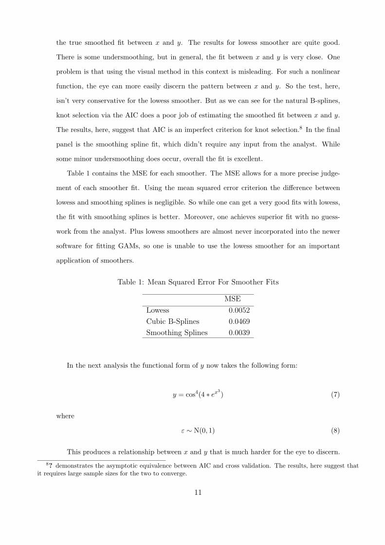
the true smoothed fit between x and y. The results for lowess smoother are quite good.

There is some undersmoothing, but in general, the fit between x and y is very close. One

problem is that using the visual method in this context is misleading. For such a nonlinear

function, the eye can more easily discern the pattern between x and y. So the test, here,

isn’t very conservative for the lowess smoother. But as we can see for the natural B-splines,

knot selection via the AIC does a poor job of estimating the smoothed fit between x and y.

The results, here, suggest that AIC is an imperfect criterion for knot selection.8 In the final

panel is the smoothing spline fit, which didn’t require any input from the analyst. While

some minor undersmoothing does occur, overall the fit is excellent.

Table 1 contains the MSE for each smoother. The MSE allows for a more precise judge-

ment of each smoother fit. Using the mean squared error criterion the difference between

lowess and smoothing splines is negligible. So while one can get a very good fits with lowess,

the fit with smoothing splines is better. Moreover, one achieves superior fit with no guess-

work from the analyst. Plus lowess smoothers are almost never incorporated into the newer

software for fitting GAMs, so one is unable to use the lowess smoother for an important

application of smoothers.

Table 1: Mean Squared Error For Smoother Fits

MSE

Lowess 0.0052

Cubic B-Splines 0.0469

Smoothing Splines 0.0039

In the next analysis the functional form of y now takes the following form:

y = cos4(4 ∗ ex3) (7)

where

ε ∼ N(0, 1) (8)

This produces a relationship between x and y that is much harder for the eye to discern.

8? demonstrates the asymptotic equivalence between AIC and cross validation. The results, here suggest thatit requires large sample sizes for the two to converge.

11

0.0 0.2 0.4 0.6 0.8 1.0

0.0

0.4

0.8

1.2

True Fit

X

Y

0.0 0.2 0.4 0.6 0.8 1.00.

00.

40.

81.

2

Lowess

X

Y

0.0 0.2 0.4 0.6 0.8 1.0

0.0

0.4

0.8

1.2

Natural Cubic B−spline

X

Y

0.0 0.2 0.4 0.6 0.8 1.0

0.0

0.4

0.8

1.2

Smoothing Splines

X

Y

Figure 1: A Comparison of Estimated Smoother Fits.

12

A scatterplot of the two variables is in Figure 2 along with the true fit between x and y.

Here, visual identification of how smooth the relationship between x and y is will be much

more difficult.

0.0 0.2 0.4 0.6 0.8 1.0

−3

−2

−1

01

23

X

Y

Figure 2: A Simulated Nonlinear Smooth Functional Form

In Figure 3 I plot a lowess fit with six different bandwidths along with a smoothing spline

fit done with automatic parameter selection. In general, the lowess produces a variety of

fits that all roughly capture the true relationship between x and y. While one of the fits

is obviously too rough and others are too smooth, two or three produce fairly reasonable

fits and might be reasonably chosen. It is this uncertainty that will not be reflected in the

estimated confidence bands. The smoothing spline fit very closely matches the true functional

13

form, but does so with no input from the analyst and the estimation uncertainty of λ will

be reflected in the confidence bands. Finally, I plot the lowess with with the lowest MSE

against the smoothing spline fit in Figure 4.

0.0 0.2 0.4 0.6 0.8 1.0

−2

02

4

Lowess − 6 Different Spans

x

y

0.0 0.2 0.4 0.6 0.8 1.0

−2

02

4

Spline − Automatic Smoothing

x

y

Figure 3: Comparing Fits Between Smoothing Splines and Lowess with Various Bandwidths

Interesting the lowess fit with the lowest MSE (at 1.01) is a fairly rough fit and one that

would almost never be chosen by an analyst. The smoothing spline fit is quite smooth with

an MSE of 1.02. Lowess fits that are smoother have MSE values that are slightly higher than

that of the smoothing spline. The results, here, demonstrate that smoothing spline fits with

automatic parameter selection produce fits that closely match the true relationship between

x and y. Moreover, the smoothing spline fits are not jagged in any way. I, next, turn to some

empirical examples to further demonstrate how well smoothing splines perform.

4 Overdrafts and Congress Revisited

Beck and Jackman (1998) replicate an OLS model from Jacobson and Dimock (1994). The

14

0.0 0.2 0.4 0.6 0.8 1.0

−3

−2

−1

01

23

x

y

Smoothing SplineLowess, Span = 0.1

Figure 4: Lowess Fit Chosen By MSE and Smoothing Spline Fit

15

model they replicate demonstrates how the number of overdrafts in the House banking scandal

affected the challengers vote share in the 1992 Congressional elections. They use a GAM

to replace a logarithmic term for the number of overdrafts with a smoothed loess fit. To

demonstrate that using automatic smoothing techniques produces no greatly different fit

with real data, I plot in Figure 5 spline fits with varying degrees of freedom and a smoothing

spline fit where the smoothing parameter was estimated via GCV.

0 200 400 600 800

05

1015

Automatic Selection

Number of Overdrafts

Cha

nge

In C

halle

nger

’s V

ote

Sha

re

0 200 400 600 800

−5

05

10

DF = 2

Number of Overdrafts

Cha

nge

In C

halle

nger

’s V

ote

Sha

re

0 200 400 600 800

05

1015

DF = 3

Number of Overdrafts

Cha

nge

In C

halle

nger

’s V

ote

Sha

re

0 200 400 600 800

−5

05

1015

DF = 4

Number of Overdrafts

Cha

nge

In C

halle

nger

’s V

ote

Sha

re

Figure 5: Manual Fitting Compared to Automatic Selection For Overdrafts

The first panel of Figure 5 contains a plot where the amount of smoothing was estimated

16

by GCV. First, these is no sign of undersmoothing or a jagged fit. Second, the fit is also

not highly nonlinear. While there are some minor differences, we observe the same pattern

where the effect of the number of overdrafts on challenger’s vote share levels off once a

threshold is met. The confidence bands for the smoothing spline are also more accurate as

they reflect estimation uncertainty for λ, while for the other fits, the confidence bands do not

take this uncertainty into account. The evidence, here, suggests that automatic smoothing

parameter selection produces fits that are equally smooth as user selected fits but appeal to

data instead of guesswork. Moreover, the smoothing spline fit produces confidence bands that

more accurately reflect our uncertainty. I, next, examine automatic smoothing parameter

selection in a different empirical context.

5 Smoothing Time For Binary TSCS

One area of political science where splines are frequently used is in the analysis of binary

time-series cross sectional data. As Beck, Katz and Tucker (1998) demonstrate, including

a smoothed time counter on the right had side of a logit model will account for duration

dependence in such data. While a number of functional forms for time are possible, they

recommend using natural cubic splines for fitting such models. Of course, while natural cubic

splines are a reasonable choice, they do require the analyst to choose the number of knots.

This is an area where analysts are are unlikely to have strong prior convictions about the

number of knots required. Smoothing splines, of course, relax the requirement that analysts

make decisions about the number of knots or the degree of smoothing. Here, I examine

whether using smoothing splines improves the overall fit of the model versus having the

analyst choose the number of knots.

Performing such a test is quite simple. The model with cubic splines and the smoothing

spline model are nested which implies that a likelihood ratio test between the model with

analyst chosen knots and a model that uses smoothing splines will tell us whether there is

any statistically significant difference between the two models.9. For the test I re-estimate

9The models are only approximately nested, but most texts argue that while the likelihood ratio test is onlyapproximate, it is still reasonably accurate (Ruppert, Wand and Carroll 2003; Wood 2006)

17

the logit model with natural cubic splines from Beck, Katz and Tucker (1998)10. I then

estimated the same model using smoothing splines and used GVC for the selection of the

smoothing parameter. I then performed a likelihood ratio test. I do not present the specific

results from the two models, which are immaterial, but the results from the likelihood ratio

test are in Table 2.

Table 2: Likelihood Ratio Test Between Cubic and Smoothing Splines

T-statistic 8.76

p-value 0.01

χ2, df ≈ 2

The use of smoothing splines improves the overall fit of the model considerably, as we

are able to reject the null that the extra parameters in the smoothing spline model are

unnecessary at the 0.01 level. Here, then, smoothing splines remove the uncertainty about

the number of knots while also improving the overall fit of the model.11

6 Diagnostic Hazard Plots

Smoothers are also important tools for the examination of diagnostic plots. Here, the eye can

be deceived by what may or may not be a pattern in the plot, while smoothers can help reveal

patterns and detect nonlinearities. But with residual plots, the analyst is unlikely to have

any theory to guide the number of knots or the degree of smoothing necessary. Moreover,

with splines not enough knots or undersmoothing can make a pattern appear linear when we

are trying to detect nonlinearity. In such situations, it is far better to rely on an automatic

smoothing procedure and let the data, typically in the form of model residuals, speak for

itself.

One diagnostic where we might want to use smoothing splines is in the detection of non-

proportional hazards when using the Cox model for duration data. Box-Steffensmeier and10Beck et al. estimate several models with splines. I only reestimated the logit spline model from Table 1.11The only cost comes in the form of the software used. Smoothing splines are currently unavailable in Stata.

I should also note that Beck, Katz and Tucker (1998) advise that they forgo the use of smoothing splines so thatthe analysis can be conducted in Stata. Presumably had they used smoothing splines, they would not have usedthem in conjunction with automatic smoothing parameter selection given they objections raised in Beck, Katz andTucker (1998).

18

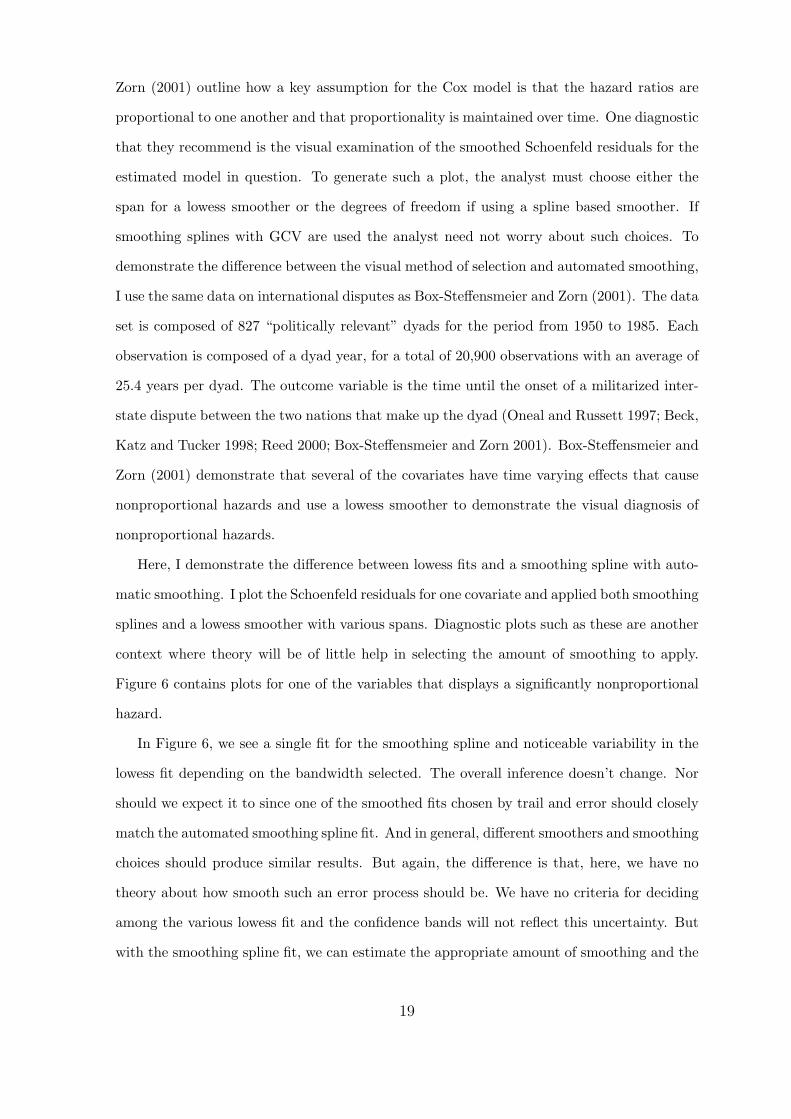
Zorn (2001) outline how a key assumption for the Cox model is that the hazard ratios are

proportional to one another and that proportionality is maintained over time. One diagnostic

that they recommend is the visual examination of the smoothed Schoenfeld residuals for the

estimated model in question. To generate such a plot, the analyst must choose either the

span for a lowess smoother or the degrees of freedom if using a spline based smoother. If

smoothing splines with GCV are used the analyst need not worry about such choices. To

demonstrate the difference between the visual method of selection and automated smoothing,

I use the same data on international disputes as Box-Steffensmeier and Zorn (2001). The data

set is composed of 827 “politically relevant” dyads for the period from 1950 to 1985. Each

observation is composed of a dyad year, for a total of 20,900 observations with an average of

25.4 years per dyad. The outcome variable is the time until the onset of a militarized inter-

state dispute between the two nations that make up the dyad (Oneal and Russett 1997; Beck,

Katz and Tucker 1998; Reed 2000; Box-Steffensmeier and Zorn 2001). Box-Steffensmeier and

Zorn (2001) demonstrate that several of the covariates have time varying effects that cause

nonproportional hazards and use a lowess smoother to demonstrate the visual diagnosis of

nonproportional hazards.

Here, I demonstrate the difference between lowess fits and a smoothing spline with auto-

matic smoothing. I plot the Schoenfeld residuals for one covariate and applied both smoothing

splines and a lowess smoother with various spans. Diagnostic plots such as these are another

context where theory will be of little help in selecting the amount of smoothing to apply.

Figure 6 contains plots for one of the variables that displays a significantly nonproportional

hazard.

In Figure 6, we see a single fit for the smoothing spline and noticeable variability in the

lowess fit depending on the bandwidth selected. The overall inference doesn’t change. Nor

should we expect it to since one of the smoothed fits chosen by trail and error should closely

match the automated smoothing spline fit. And in general, different smoothers and smoothing

choices should produce similar results. But again, the difference is that, here, we have no

theory about how smooth such an error process should be. We have no criteria for deciding

among the various lowess fit and the confidence bands will not reflect this uncertainty. But

with the smoothing spline fit, we can estimate the appropriate amount of smoothing and the

19

0 5 10 15 20 25 30 35

−2

−1

01

23

Time

Pre

viou

s D

ispu

tes

Figure 6: Plot of Schoenfeld Residuals With Lowess and Smoothing Spline Fits

20

confidence bands will reflect this estimation uncertainty.

7 Conclusion

Smoothers are an important component of analysts’ toolkit. They can be used to estimate

nonlinear effects in parametric models, control for duration dependence in binary time series

cross sectional datasets, smooth hazards, reveal functional forms in scatterplots, and aid in

the testing of model assumptions.

But given the variety of smoothers and the choices required when using each smoother, the

results from using smoothers can appear arbitrary. While, in fact, for most smoothers, only

one choice really matters–the choice of bandwidth or equivalently the degrees of freedom–

that choice can still engender controversy. Undoubtedly, some of the controversy stems from

the visual method of making this choice. But as I have demonstrated, often there is no

need to resort to visual methods when using smoothers. Smoothing splines with automatic

smoothing parameter selection allow the analyst to estimate smoothed fits that rely on the

data itself to select the amount of smoothing. They also produce confidence bands that

better reflect our uncertainty about how smooth a process is.

Of course, analysts should not rely solely on automatic parameter selection. If they, in

fact, have a theory about the level of smoothness or the results from automatic selection

seem overly nonlinear or rough, they can then select the amount of smoothing. Moreover,

plotting some manually selected smoothed fits versus one chosen via GVC or REML serves

as a useful diagnostic to ensure that the automatic fit isn’t unusually rough or too nonlinear.

But barring theoretical concerns, analysts are often better off letting the amount of

smoothing be estimated from the data. Automatic smoothing removes any hint of art from

the process, and more importantly provides confidence bands that more accurately reflect our

uncertainty about the level of smoothness. As I have demonstrated, automatic smoothing

produces excellent fits in simulated data and good estimates with real data. So in short, there

are no real objections to use automatic smoothers and more importantly several reasons that

we should be using them.

21

References

Beck, Neal, Jonathan N. Katz and Richard Tucker. 1998. “Taking Time Seriously: Time-Series-Cross-Section Analysis with a Binary Dependent Variable.” American Journal ofPolitical Science 42:1260–1288.

Beck, Neal and Simon Jackman. 1998. “Beyond Linearity by Default: Generalized AdditiveModels.” American Journal of Political Science 42:596–627.

Box-Steffensmeier, Janet M. and Bradford S. Jones. 2004. Event History Modeling: A Guidefor Social Scientists. New York: Cambridge University Press.

Box-Steffensmeier, Janet M. and Christopher J. W. Zorn. 2001. “Duration Models andProportional Hazards in Political Science.” American Journal of Political Science 45:972–988.

Eilers, Paul H.C. and Brian D. Marx. 1996. “Flexible Smoothing with B-splines and Penal-ties.” Statistical Science 11:98–102.

Fox, John. 1997. Applied Regression Analysis, Linear Models, and Related Methods. Thou-sand Oaks, CA: Sage.

Fox, John. 2000. Nonparametric Simple Regression. Thousand Oaks, CA: Sage.

Hastie, T.J. 1996. “Pseudosplines.” Journal of The Royal Statistical Society, Series B 58:379–396.

Hastie, T.J. and R.J. Tibshirani. 1990. Generalized Additive Models. London: Chapman andHall.

Jacobson, Gary C. and Michael Dimock. 1994. “Checking Out: The Effects of Bank Over-drafts on the 1992 House Elections.” American Journal of Political Science 38:601–624.

Keele, Luke. 2006. “Covariate Functional Form In Cox Models.” Working Paper.

Oneal, John R. and Bruce Russett. 1997. “The Classial Liberals Were Right: Democracy,Interdependence, and Conflict, 1950-1985.” International Studies Quarterly 41:267–294.

Reed, William. 2000. “A Unified Statistical Model of Conflict and Escalation.” AmericanJournal of Political Science 44:84–93.

Ruppert, David, M.P. Wand and R.J. Carroll. 2003. Semiparametric Regression. New York:Cambridge University Press.

Silverman, B.W. 1985. “Some Aspects of the Spline Smoothing Approach to NonparametricRegression Curve Fitting.” Journal of the Royal Statistical Society, Series B 47:1–53.

Stone, C.J. 1986. “Comment: Generalized Additive Models.” Statistical Science 2:312–314.

Wahba, G. 1983. “Bayesian Confidence Intervals For the Cross Validated Smoothing Spline.”Journal of the Royal Statistical Society, Series B 45:133–150.

Wahba, G. 1990. Spline Models for Observational Data. Philadelphia: SIAM.

Wood, Simon. 2006. Generalized Additive Models: An Introduction With R. Boca Raton:Chapman & Hall/CRC.

22