How the Electoral College Influences

Campaigns and Policy:

The Probability of Being Florida

Forthcoming American Economic Review, June 2008.

David Strömberg∗

IIES, Stockholm University

Abstract

This paper analyzes how US presidential candidates should allocate resources across states to

maximize the probability of winning the election, by developing and estimating a probabilistic-

voting model of political competition under the Electoral College system. Actual campaigns

act in close agreement with the model. There is a 0.9 correlation between equilibrium and

actual presidential campaign visits across states, both in 2000 and 2004. The paper shows how

presidential candidate attention is affected by the states’ number of electoral votes, forecasted

state-election outcomes, and forecast uncertainty. It also analyzes the effects of a direct national

popular vote for president.

∗david.stromberg@iies.su.se, IIES, Stockholm University, S-106 91 Stockholm.I thank Steven Brams, Steve Coate, Antonio Merlo, Torsten Persson, Gerard Roland, Tom Romer, Howard Rosenthal, JimSnyder, Jörgen Weibull, and seminar participants at UC Berkeley, Columbia University, Cornell University, the CEPR/IMOPConference in Hydra, Georgetown University, the Harvard / MIT Seminar on Positive Political Economy, IIES, New YorkUniversity, Stanford University, University of Pennsylvania, Princeton University, and the Wallis Conference in Rochester, theeditor and three anonymous referees. Previous versions have been circulated under the titles: ”The Lindbeck-Weibull model inthe Federal US Structure”, and, ”The Electoral College and Presidential Resource Allocation”, and "Optimal Campaigning inPresidential Elections: The Probability of Being Florida.".JEL-classification, D72, C50, C72, H50, M37.Keywords: elections, political campaigns, public expenditures

1. Introduction

The President of the United States is arguably the world’s most powerful political leader, and the

incentives created by his electoral procedure are important. In consequence, it is not surprising

that the Electoral College system of electing president1 has been under constant debate. According

to federal historians, over 700 proposals have been introduced in Congress in the last 200 years

to reform or eliminate the Electoral College system. Indeed, there have been more proposals for

constitutional amendments to alter or abolish the Electoral College than on any other subject.

The drive toward reform is understandable given the perceived impact on the democratic process

and economic policy. For example, voters in states like Utah, Massachusetts, and Idaho did not see

much of Bush and Kerry in person or in advertisements, while more than 3 of every 5 candidate

visits in 2004 went to Florida, Ohio, Wisconsin, Iowa and Pennsylvania. This leaves people in the

former states feeling neglected, and with weaker incentives to get informed and to vote. Equally

worrying are the fears that the Electoral College might induce distorted and inefficient government

policies.2 This debate is as old as the Constitution.3 Still, the overwhelming part of previous work

on redistributive politics in the U.S. has been concerned with Congress, neglecting the role of the

President. An important exception is a set of early game-theoretic analyses of the Electoral College

system, following Brams and Davis (1974).

The goal of the current paper is to provide answers to a set of questions regarding the impact of

the Electoral College. The developed model of electoral competition first gives a precise answer to

1When U.S. citizens vote for President and Vice President, ballots show the names of the Presidentialand Vice Presidential candidates, although they are actually electing a slate of "electors" that representthem in each state. After the election, the party that wins the most votes in each state appoints all of theElectors for that state (except in Maine and Nebraska). The number of Electors equals the state’s numberof U.S. Senators (always 2) plus the number of its U.S. Representatives (increasing in the State’s populationas determined in the Census). The electors from every state combine to form the Electoral College. TheElectors cast their votes and sent to the President of the Senate. On January 6, the President of the U.S.Senate opens all of the sealed envelopes containing the Electoral votes and reads them aloud. To be electedas President or Vice President, a candidate must have an absolute majority of the Electoral votes for thatposition.

2See for example, Susan Page, "Bush policies follow politics of states needed in 2004", USA Today, June 16,2002; or John Mercurio, "Bush stumps in Rust Belt. On the verge of repealing steel tariffs", CNN, December2, 2003; or Carl Hulse and Matthew L. Wald, "President’s Response to Hurricane Carries Reminders ofPolitical Fallout for Past Candidates", New York Times, August 15, 2004.

3For example, in the Federalist Papers (#64), John Jay discusses the "fears and apprehensions of some,that the President and Senate may make treaties without an equal eye to the interests of all the States."

2

how presidential candidates should allocate campaign resources across states to win the presidential

election. The model explains why candidate resources are so concentrated, and, in general, what

determines how concentrated they will be. It also identifies the states — like Florida, Ohio, and

Iowa in 2004 — that should receive most attention in each election, by deriving an analytic formula

determining how attention is related to the number of electoral votes, opinion polls, and other

variables available in September of the election year. The number of times the candidate should

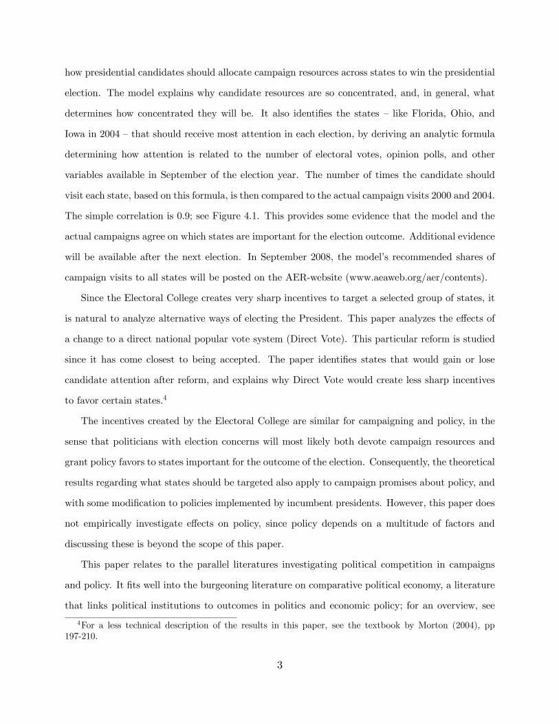
visit each state, based on this formula, is then compared to the actual campaign visits 2000 and 2004.

The simple correlation is 0.9; see Figure 4.1. This provides some evidence that the model and the

actual campaigns agree on which states are important for the election outcome. Additional evidence

will be available after the next election. In September 2008, the model’s recommended shares of

campaign visits to all states will be posted on the AER-website (www.aeaweb.org/aer/contents).

Since the Electoral College creates very sharp incentives to target a selected group of states, it

is natural to analyze alternative ways of electing the President. This paper analyzes the effects of

a change to a direct national popular vote system (Direct Vote). This particular reform is studied

since it has come closest to being accepted. The paper identifies states that would gain or lose

candidate attention after reform, and explains why Direct Vote would create less sharp incentives

to favor certain states.4

The incentives created by the Electoral College are similar for campaigning and policy, in the

sense that politicians with election concerns will most likely both devote campaign resources and

grant policy favors to states important for the outcome of the election. Consequently, the theoretical

results regarding what states should be targeted also apply to campaign promises about policy, and

with some modification to policies implemented by incumbent presidents. However, this paper does

not empirically investigate effects on policy, since policy depends on a multitude of factors and

discussing these is beyond the scope of this paper.

This paper relates to the parallel literatures investigating political competition in campaigns

and policy. It fits well into the burgeoning literature on comparative political economy, a literature

that links political institutions to outcomes in politics and economic policy; for an overview, see

4For a less technical description of the results in this paper, see the textbook by Morton (2004), pp197-210.

3

Persson and Tabellini (2000). It is particularly closely related to Lizzeri and Persico (2001), Persson

and Tabellini (1999), and Milesi-Ferreti et al. (2002) who compare taxes, spending and transfers

in polities with majoritarian and proportionally representative electoral rules. For an overview of

results regarding the policy impact of political US institutions on policy, see Besley and Case (2003).

The current paper also relates to the literature on campaigning, in particular to Brams and Davis

(1974). These authors analyze how presidential candidates should allocate campaign resources

across states to maximize their expected electoral vote. They find that presidential candidates

should allocate resources disproportionately in favor of large states, if each candidate wins every

state with equal probability and the number of undecided voters is proportional to the number of

electoral votes. This result is disputed by Colantoni, Levesque and Ordeshook (1975) who instead

argue that a proportional rule, modified to take into account the ex post closeness of the state

election, predicts actual campaign allocations better. Also closely related is Snyder’s (1989) model

of two-party competition for legislative seats that allows for variation in vote shares and where

candidates maximize the chance of winning.

A major difference between this paper and earlier work is the complete integration of theory

and empirics, tying together theoretical insights with empirical results on actual campaigns. This

can be done since the constructed probabilistic-voting model is sufficiently general to be directly

applied to the real world problem of a U.S. presidential candidate, yet can be explicitly solved, and

directly estimated. This framework allows for new questions to be asked and answered.

More specifically, the model of this paper differs from that of Brams and Davis (1974) in allowing

states to have different partisan leanings, in allowing for uncertainty regarding the election outcome

at both state and national level, and in having the candidates maximizing the probability of winning

instead of their expected electoral vote. It differs from the model of Snyder (1989) in allowing for

different state sizes, uncertainty at both state and national level, and in providing closed-form

solutions. While Persson and Tabellini (1999) use a similar probabilistic-voting framework, they

only have three states, each with one vote, and no state-level uncertainty. Perhaps the set-up of

Lizzeri and Persico’s (2001) model is most different. They use a continuum of states, each with one

electoral vote, and let votes be entirely decided by campaign efforts (no uncertainty). However, the

4

models of Persson and Tabellini (1999) and Lizzeri and Persico (2001) allow the candidates to use

richer strategies, setting taxes and public spending in addition to targeted spending.

The model finally demonstrates that there is a link between all of the above literature and

the literature concerning “voting power”, that is, the probability that a vote is decisive in an

election. The statistical properties of voting power have been analyzed extensively; see Banzaf

(1968), Chamberlain and Rothschild (1988), Gelman and Katz (2001), Gelman, King and Boscardin

(1998)), and Merrill (1978). The “voting power” analyzed in this paper is slightly different since it

is conditional on the candidates’ equilibrium strategies.

The theoretical model of presidential campaigning is developed in Section 2. The model is esti-

mated in Section 3, using data from presidential elections 1948-2004. This answers the question of

how candidates should have allocated campaign resources across states to maximize the probability

of winning. Section 4 studies whether presidential campaign visits in the 2000 and 2004 elections

resemble those recommended by theory. Section 5 shows that the rather complex equilibrium condi-

tion has a very intuitive meaning. It also answers questions such as: do large or small states benefit

from the electoral college system; what would happen if opinion polls were not allowed; should

50-50 states receive most attention? Section 6 discusses the impact of electoral reform. Section 7

concludes.

2. Model

2.1. Setup

We begin by assuming that there are two presidential candidates, indexed by superscript R and D,

for now ignoring the impact of minority-party candidates. Both candidates have to make campaign

plans for the last I days before the election.5 The plans specify how many of the I days to use

to visit each of S states (in 2004, S equaled 51, including the 50 states and Washington D.C.).

Formally, let dJs represent the number of days candidate J = R,D visits state s. Each candidate J

5Historically, presidential campaigns have begun around Labor Day and end on election day, althoughcandidates often start campaigning as soon as nomination is secured.

5

chooses dJs subject to the constraintSXs=1

dJs ≤ I. (2.1)

We assume that the objective of the candidates is to maximize their probability of winning the

election. Of course, candidates may have other goals in campaigning, such as helping out congres-

sional or senatorial candidates or candidates in state and local races. But, at least in close races,

maximizing the probability of winning is likely to be the main concern.

How the election result is affected by campaign visits depends on how voters respond, and the

formal electoral rules. Starting with the latter, each state s is allocated a number of electoral votes,

es. In practice, es equals the state’s number of U.S. Senators (always 2) plus the number of its U.S.

Representatives (increasing in the State’s population as determined in the Census). In each state,

there is a popular election. The candidate who receives a majority of the votes in a state s gets

all the es electoral votes of that state.6 After elections have been held in all states, the electoral

votes are counted, and the candidate who gets more than half those votes wins the election. The

model ignores that in two states, Maine and Nebraska, two electoral votes are chosen by statewide

popular vote and the remainder by the popular vote within each Congressional district.7

Turning to voter behavior, we assume that campaign visits by presidential candidates matter —

they affect how voters choose on election day.8 Formally, the increasing popularity of candidate J

campaigning dJs days in state s, is captured by the increasing and concave function u¡dJs¢. This

implies that the effect of visits decreases with the number of visits.

Vote choices, of course, depend on things other than candidate visits. Voters are affected by

the candidates’ divergent policy positions, and perhaps candidate appearance. We will call all these

6The model ignores that the, presently, 538 individuals (one for each electoral vote) that actually vote forthe president in the Electoral College are not formally bound to vote for the candidate for which they havepledged support. There have been 8 "faithless electors" in this century, and as recently as 2004 a DemocratElector in the State of Minnesota cast his votes for John Edwards instead of Presidential candidate JohnKerry. However, faithless electors have never changed the outcome of an election, most often it seems thattheir purpose is to make a statement rather than make a difference.

7This method has been used in Maine since 1972 and Nebraska since 1996, though since both states haveadopted this modification, the statewide winners have consistently swept all of the state’s districts as well.Consequently, neither state has ever split its electoral votes.

8This paper does not address the question of why campaigning matters. This is an interesting questionin its own right, with many similarities to the question of why advertisements affect consumer choice. For adiscussion of how visits matter and empirical evidence that they do, see Morton (2005).

6

other factors for ideological preferences and treat them as exogenous. Key to the model is that at

the time campaign strategies are chosen, the candidates are uncertain about the voters ideological

preferences on election day. This uncertainty arises both because the true preferences of the voters

at the time campaign plans are made are not known, and because of the realization of stochastic

events after plans are made which shift voter preferences. Some of this uncertainty affects all voters

in a similar way and create national swings. For example, in 1980 a U.S. government attempt to

rescue hostages in Iran ended in a helicopter crash that killed eight servicemen. Voter evaluations

of president Carter’s performance fell across the nation. Other uncertainty is state-specific and

generates swings in only one state. For example, the unexpected downturn in a state’s economy

may shift voter preferences for government spending and unemployment insurance.

These features are modeled by writing the ideological preferences of the voters as a sum of three

parts — Ri, ηs, and η — where Ri is predictable at the time the campaign plans are made, and η

and ηs are the unpredictable national and state swings. The predictable part of voters’ ideological

preferences within each state is normally distributed, with a mean which may shift over time but

with a constant variance, specifically,

Ri ∼ Fs = N¡µs, σ

2fs

¢. (2.2)

The S state-level popularity parameters, ηs, and the national popularity parameter, η, are indepen-

dently drawn from the distributions

ηs ∼ Gs = N(0, σ2s),

and

η ∼ H = N¡0, σ2

¢.

The voters may vote for candidate R or candidate D. Considering campaigning and ideological

preferences, a voter i in state s will vote for candidate D if

u¡dDs¢− u

¡dRs¢= ∆us ≥ Ri + ηs + η, (2.3)

7

where the first equality defines ∆us. Consequently, the share of votes, ys, that candidate D receives

in state s on election day when the candidates have chosen strategies resulting in ∆us and after the

shocks ηs and η have been realized is

ys = Fs(∆us − ηs − η). (2.4)

2.2. The approximate probability of winning

We now turn to computing the approximate probability of winning the presidential election, given

any set of campaign strategies chosen by the two candidates. Candidate D wins a particular state

s if

ys ≥1

2,

or, equivalently, if

ηs ≤ ∆us − µs − η.

The probability of this event, conditional on the aggregate popularity η, and the campaign visits,

dDs , and dRs , is

Gs (∆us − µs − η) . (2.5)

Let es be the number of votes of state s in the Electoral College. Define the stochastic variables,

Ds, that indicate whether D wins state s

Ds = 1, with probability Gs (·) ,

Ds = 0, with probability 1−Gs (·) .

Let ∆u = (∆u1,∆u2, ...,∆uS) be the utility differentials resulting from any allocation of campaign

resources across states of the two campaigns. The probability that D wins the election for any

national popularity shock, η, and utility differentials from campaigning is then

ePD (∆u, η) = Pr

"Xs

Dses >1

2

Xs

es

#. (2.6)

8

However, it is difficult to find strategies which maximize the expectation of the above probability

of winning. The reason is that it is a sum of the probabilities of all possible combinations of state

election outcomes which would result in D winning. The number of such combinations is of the

order of 251, for each of the infinitely many realizations of η.

A way to cut this Gordian knot, and to get a simple analytical solution to this problem, is

to assume that the candidates are considering their approximate probabilities of winning.9 Since,

given the national shock η, the ηs are independent, and so are the Ds. Therefore by the Central

Limit Theorem of Liapounov,10 PsDses − µ

σE,

where

µ = µ (∆u, η) =Xs

esGs (∆us − µs − η) , (2.7)

and

σ2E = σ2E (∆u, η) =Xs

e2sGs (·) (1−Gs (·)) , (2.8)

is asymptotically distributed as a standard normal. The mean, µ, is the expected number of elec-

toral votes. That is, the sum of the electoral votes of each state, multiplied by the probability of

winning that state. The variance, σ2E, is the sum of the variances of the state outcomes, which is

the e2s multiplied by the usual expression for the variance of a Bernoulli variable. Using the asymp-

totic distribution, the approximate probability of D winning the election, for any given national

popularity shock and utility differentials from campaigning, is

ePD (∆u, η) = 1−Φ"12

Ps es − µ (∆u, η)

σE (∆u, η)

#, (2.9)

9Lindbeck and Weibull (1987) uses this trick in a different setting.10See, for example, Ramanathan (1993), p. 157. The formal requirements for convergence are

Eh|Dses − µs|

2+δi= ρs for some δ > 0 and lim

S→∞( S

s=1 ρs)2

( Ss=1 σ

2s)

2+δ = 0. For our purposes, it is more inter-

esting to know the approximation error using our sample (51 states in the elections 1948-2004) than thelimiting behavior. The distributions of election outcomes using the approximation are plotted together withthe outcomes not using the approximation in Appendix 6.8 of Stromberg (2002). From the presidentialcandidates’ point of view, the relevant statistic is the error that they make by maximizing the approximateprobability of winning. This error is discussed in Section 5.

9

where Φ [·] is the standard normal cumulative density function. The approximate probability of

winning as a function of campaigning only is found by taking the expectation over the national

popularity shocks,

PD (∆u) =

Z ePD (∆u, η)h (η) dη. (2.10)

2.3. Equilibrium

Having derived the approximate probability of winning we now characterize the Nash Equilibrium.

The equilibrium strategies¡dD∗, dR∗

¢are characterized by

PD¡dD∗, dR

¢≥ PD

¡dD∗, dR∗

¢≥ PD

¡dD, dR∗

¢for all dD, dR in X, the set of allowable campaign visits,

X =

(d ∈ <S

+ :SXs=1

ds ≤ I

).

This game has a unique interior pure-strategy equilibrium characterized by the proposition below.

Proposition 1. The unique pair of strategies for the candidates¡dD, dR

¢that constitute an interior

NE in the game of maximizing the expected probability of winning the election must satisfy dD =

dR = d∗, and, for all s and for some λ > 0,

Qsu0 (d∗s) = λ, (2.11)

where

Qs =∂PD

∂∆us. (2.12)

Proof: See Appendix 8.1.

Proposition 1 says that presidential candidates should spend more time in states with high

values of Qs. This follows since u0 (d∗s) is decreasing in d∗s. In the empirical section, u0 (0) will be

assumed to be sufficiently high that the equilibrium is interior.

10

Note that Qs consists of two additively separable parts:

Qs = Qsµ +Qsσ (2.13)

= es

Z1

σEϕ (x (η)) gs (−µs − η)h (η) dη

+e2sσ2E

Zϕ (x (η))x (η)

µ1

2−Gs (−µs − η)

¶gs (−µs − η)h (η) dη,

where

x (η) =12

Ps es − µ

σE,

and ϕ (·) is the standard normal probability density function. The first arises because the candidates

have an incentive to influence the expected number of electoral votes won by D, that is the mean of

the normal distribution. The second arises because the candidates have an incentive to influence the

variance in the number of electoral votes. This variance matters since they maximize the probability

of winning, which is a locally convex (concave) function for the trailing (leading) candidate; for

further discussion, see Section 5.4.

The value of Qs depends only on the parameters es, µs, and σs, for all states s = 1, 2, ..., S, and

σ,

Qs = Qs (e1, e2, ..., eS, µ1, µ2, ..., µS , σ1, σ2, ..., σS, σ) . (2.14)

This can be seen by inserting the definitions of σ2E, µ, gs (·) , and h (·) in equation (2.13). The

distribution of electoral votes, es, is known. To determine the value of Qs for each state in each

election, we now estimate the remaining parameters.

3. Estimation

Estimation of µs, σs, and σ, provides the link between the theoretical probabilistic-voting model

above and the empirical applications discussed below. Intuitively, estimation amounts to predicting

state-level Democratic vote shares 1948-2004 (µs) using a set of observables, and then estimating

the national, and independent state-level, uncertainty in this prediction (σ and σs). Since we are

using a panel, let t denote time, and s state, subscripts.

11

Formally, both candidates choose the same allocation in equilibrium, so that ∆ust = 0 in all

states. The Democratic vote-share in state s at time t equals, using equations (2.4) and (2.2),

yst = Fst (−ηst − ηt) = Φ

µ−µst − ηst − ηt

σfs

¶, (3.1)

where Φ (·) is the standard normal distribution, or equivalently,

Φ−1(yst) = γst = −1

σfs(µst + ηst + ηt) . (3.2)

For now, assume that all states have the same variance of preferences, σ2fs = 1, and the same

variance in state-specific shocks, σ2s.11 Further assume that the predicted mean of the ideological

preference distribution, µst, depends linearly on a set of observable variables

µst = x1stβ1 + x2stβ2 + ...+ xKstβK = Xstβ.

Then we get the following estimable equation,

γst = − (Xstβ + ηst + ηt) . (3.3)

The parameters β, σs and σ are estimated using a standard maximum-likelihood estimation of the

above time random-effects model.12

The variables in Xst are basically those used in Campbell (1992). Table A1 lists all variable

definitions and sources, and Table 1 displays the summary statistics. The nation-wide variables are:

the Democratic vote share of the two-party vote share in trial-heat polls from mid September (all

11These assumptions will be removed in Section 6. However, the estimates become imprecise if separatevalues of µst, σfs, and σs are estimated for each state using only 15 observations per state. Therefore, themore restrictive specification will be used for most of the paper.12The model has been extended to include regional swings, see Appendix 6.4 of Strömberg (2002). In this

specification, the democratic vote-share in state s equals

yst = Fst (ηst + ηrt + ηt) ,

where ηrt denotes independent popularity shocks in the Northeast, Midwest, West, and South. However,taking into account the information of September state-level opinion polls, there are no significant regionalswings. Therefore, the simpler specification without regional swings is used below.

12

vote-share variables x used in the transformed form, Φ−1(x)); the lagged Democratic vote share of

the two-party vote share; second quarter economic growth; incumbency; and incumbent president

running for re-election. The statewide variables for 1948-1984 are: lagged and twice lagged difference

from the national mean of the Democratic two-party vote share; the first quarter state economic

growth; the average ADA-scores of each state’s Congress members the year before the election; the

Democratic vote-share of the two-party vote in the midterm state legislative election; the home

state of the president; the home state of the vice president; and dummy variables described in

Campbell (1992). After 1984, state-level opinion-polls were available. For this period, the statewide

variables are: lagged difference from the national mean of the Democratic vote share of the two-

party vote share; the average ADA-scores of each state’s Congress members the year before the

election; and the difference between the state and national polls. Other statewide variables were

insignificant when state polls were included. The coefficients β and the variance of the state-level

popularity shocks, σ2s, are allowed to differ when opinion polls were available and when they were

not. Estimates of equation (3.3) yields forecasts by mid September of the election year.

The data set contains state elections for the 50 states 1948-2004, except Hawaii and Alaska

which began voting in the 1960 election; see Table A2. During this period there were a total of

744 state-level presidential election results. Four elections in Alaska and Hawaii were excluded

because there were no lagged vote returns. Nine elections are omitted because of idiosyncrasies in

Presidential voting in Alabama in 1948, and 1964, and in Mississippi in 1960; see Campbell (1992).

This leaves a total of 731 observations.

The estimation results are shown in Table 1. The statistics of main interest to us are

bσs,state polls = 0.073, (3.4)

bσ = 0.035,

and

bµst = Xstbβ, (3.5)

where bβ is the vector of estimated coefficients in Table 1, and the bσs is the estimated standard13

deviation of the state level shocks after 1984. Although the prediction errors are correlated across

states, the correlation is far from perfect. The standard error of the independent state shocks

corresponds to around 2.9 percent in terms of vote shares, while the standard error in the national

swings corresponds to around 1.7 percent.13

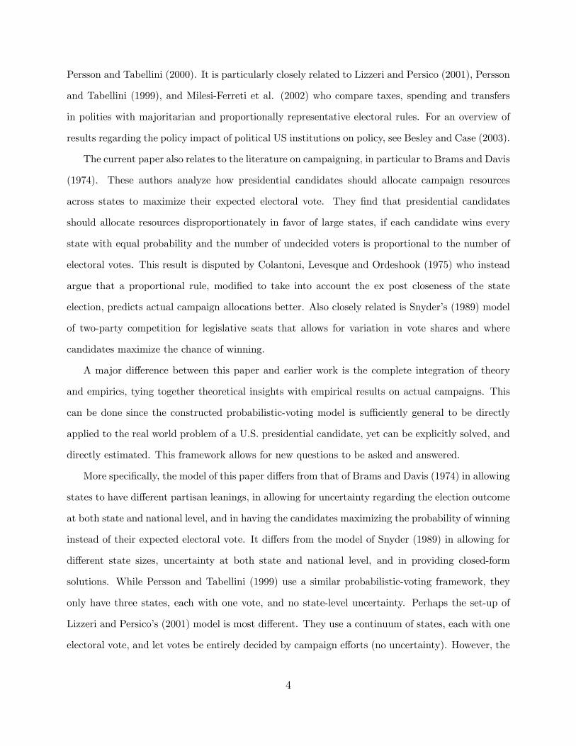
The model does well in predicting the vote-share outcomes. The average absolute error in

state-election vote-forecasts, |byst − yst| , where

byst = Φ (−bµst) , (3.6)

is 3.0 percent and the wrong winner is predicted in 13 percent of the state elections. This is

comparable to the best state-level election-forecast models (Campbell, 1992; Gelman and King,

1993; Holbrook and DeSart, 1999; Rosenstone, 1983). Table 3 shows the forecasted vote outcomes,

byst, for the last two elections. Given bµst, bσs and bσ, Qs can be calculated using equation 2.14. Table

3 also reports the computed values of Qs for the last two elections, multiplied by the constant 2√2π

for reasons explained below.

4. Relation between Qs and actual campaigns

This section discusses how the actual allocation of presidential candidate visits to states in the two

last presidential elections corresponds to the theoretical equilibrium campaigns. Both sides’ actual

post-convention campaign visits in 2000 and 2004 are reported in Table 3. The visits data was

collected by Daron Shaw and is described in Shaw (2007). I have excluded the early September

visits, since I use polling information from mid September. Visits by vice presidential candidates

are counted as 0.5 presidential candidate visits. For example, in 2000, Bush visited Florida seven

times while Cheney visited six times. Consequently, the weighted number of Republican visits to

Florida in 2000 is ten. The correlation between the Republican and Democratic campaigns’ visits

is 0.9 in both elections.

If one assumes that the impact of visits, u (ds) , is of log form, then the equilibrium number of

13Computed at bµst = 0, we get Φ (0.073)− Φ (0) = .029.

14

days spent in each state should be proportional to Qs,

state s’ share of equilibrium visits =d∗sPd∗s=

QsPQs

, (4.1)

using equation (2.11). For the elections in 2000 and 2004, each state’s equilibrium share of visits

were computed using the above equation and the estimated Qs.

The actual and equilibrium shares are shown in Figure 4.1, where both sides’ campaign visits

have been added together. For example, the actual campaigns increased the share of their visits

spent in Florida from 9 percent in 2000 to 19 percent in 2004. In comparison, QFlorida/P

Qs

increased from 11 percent in 2000 to 16 percent in 2004.

The actual campaigns closely resemble the model’s equilibrium campaigns based on September

opinion polls. The model and the candidates’ actual campaigns agree on 8 of the 10 states that

should receive most attention in both 2000 and 2004. The model and the data are also, largely, in

agreement on which states should receive basically no attention. The simple correlation between

equilibrium and actual visit shares is 0.9 in both years. A tougher comparison is that of campaign

visits per electoral vote. The correlation between ds/es and Qs/es was 0.8 in both years.

A noticeable discrepancy is that the model under-predicts the number of visits to some mid-

western states, Illinois, Iowa, Wisconsin and Missouri in 2000, and Iowa, Wisconsin and Ohio in

2004. Two plausible explanations are that my model does not include travel costs and that the

campaigns use polling data of better quality and of later date than mid September. Other factors

the model does not account for are the geographic location of the campaign headquarter and the

perceived effectiveness of campaigns in different states, depending, for example, on the support from

Governors in the campaign. (I talked extensively about this with campaigners, in particular, Daron

Shaw who worked on the Republican side in the 2000 election, and Samuel Popkin who worked on

the Democratic side in the 1992, 1996 and 2000 elections).

There is of course a lot of persistence in which states receive attention. Florida, Pennsylvania,

Michigan and Ohio are at the top in both elections. Still, while for example California and Tennessee

were high on the list in 2000, they had fallen substantially in 2004. The model also explains these

15

0 .05 .1 .15 .2 0 .05 .1 .15 .2

District of ColumbiaUtah

TexasMassachusetts

IdahoKansas

Rhode IslandNebraskaOklahoma

HawaiiNew YorkVermont

South CarolinaWyomingAlabama

South DakotaMontana

AlaskaNorth Dakota

MaineMaryland

IndianaWest Virginia

VirginiaNew JerseyMississippi

ConnecticutDelaware

MinnesotaColorado

ArizonaNevadaGeorgia

New HampshireNorth Carolina

New MexicoKentuckyArkansas

IllinoisIowa

LouisianaOregon

WashingtonWisconsin

TennesseeMissouri

OhioPennsylvania

CaliforniaMichigan

Florida

CaliforniaDistrict of Columbia

New YorkUtah

WyomingIdaho

AlaskaNebraska

MassachusettsMontana

Rhode IslandNorth Dakota

OklahomaSouth Dakota

MississippiTexas

AlabamaKentucky

HawaiiConnecticut

South CarolinaIndianaKansas

VermontLouisianaDelawareMaryland

New JerseyGeorgia

IllinoisTennessee

NevadaColorado

ArizonaMaine

ArkansasNew Hampshire

VirginiaNorth CarolinaWest VirginiaNew Mexico

IowaOregon

MissouriWashington

MinnesotaWisconsin

OhioMichigan

PennsylvaniaFlorida

2000 2004

Equilibrium visits share Actual visits share

Graphs by year

Figure 4.1: Actual and equilibrium shares of campaign visits.

16

changes reasonably well. The correlation between the changes in equilibrium and actual visit shares

between these two years is 0.6.

Obviously, candidates would like to visit large states more frequently. However, size is not

everything as is apparent from the many large states found at the bottom of Figure 4.1. An obvious

reason for this is that some states, like Texas and New York, are clearly in one candidate’s column

and that campaigning is not likely to affect this; see Colanti, Terrence and Ordeshook (1975).

Candidates should concentrate on close races. Consistent with this idea, Florida was forecasted

to have a 49.5% Democratic vote share in 2000 and received the most attention. However, the

forecasted Democratic vote share in California was closer to 50% in 2004 than in 2000 (52% compared

to 55%). Still much less attention should be (and was) given to California in 2004. The next section

explains why. Finally, the distribution of visits seems more concentrated in 2004 than in 2000. The

five top states (in terms of visits) received 41% of all visits in 2000 and 63% of the visits in 2004.

The next section will discuss what determines the skewness of the electoral incentives.

The working paper version of this paper also analyzes the allocation of TV advertisements in

the 2000 election. The data set records a total of 174 851 advertisements that were aired across

the 75 largest media markets at a total cost of $118 million. Analyzing this problem adds two

complications, one has to account for advertisement price differentials and that media markets

cross state boundaries. The model shows that equilibrium advertisements should be proportional

to the population-weighted Qs, divided by the price of advertising, Qm/pm. Figure 4.2 plots the

equilibrium and actual advertisements. The model and the data agree on the two media markets

where most ads should be aired (Albuquerque - Santa Fe, and Portland, Oregon). These two markets

have the highest effect on the win probability per initial advertising dollars. The correlation between

actual campaign advertisement and equilibrium advertisement is 0.8. Finally, since the correlation

between price and market size is close to one (0.92), there is no significant relationship between

market size and the number of ads.Via the price, the size is instead captured in the costs. Assuming

log utility, equilibrium expenditures are proportional to Qm. Empirically, the simple correlation

between equilibrium and actual advertisement expenditures is 0.9.

A stricter comparison of the equlibrium and actual visit shares is shown in Table 4. The first

17

LexingtonDenver

Albuquerque- Santa Fe

Portland, OR

020

0040

0060

0080

00A

ctua

l Num

ber o

f Adv

ertis

emen

ts

0 2000 4000 6000 8000

Equilibrium Number of Advertisements

LexingtonDenver

Albuquerque- Santa Fe

Portland, OR

020

0040

0060

0080

00A

ctua

l Num

ber o

f Adv

ertis

emen

ts

0 2000 4000 6000 8000

Equilibrium Number of Advertisements

Figure 4.2: Equilibrium and actual number of advertisements (Sept. 1 to election day) forthe 75 largest media markets in 2000.

column contains the results from an OLS regression of actual visits shares in 2000 and 2004 on

equilibrium visit shares, that is estimations of the equation

dsPds= β

QsPQs

+ ε. (4.2)

As predicted by equation 4.1, the coefficient on equilibrium visits is significantly different from zero,

but not significantly different from one. The second column includes a number of variables that seem

intuitively likely to be correlated with candidate visits: the number of electoral votes, the closeness

of the presidential elections at the state level (measured as 50 - |% Democratic votes− 50|), and

the Democratic vote share in the election.14 The number of electoral votes and the closeness of

the elections are both significantly positively correlated with candidate visits. However, adding the

equilibrium shares completely removes the significance of the electoral votes and the closeness of the

elections, and the R-squared is 0.77 with or without them; see columns (3) and (1). The variables

are neither individually or jointly significant; the F-statistic for joint significance is 0.21 with three

14A problem here is that the Democratic vote share is endogenous to campaigning. I use the actual voteshare since it is a frequently used measure of the closeness of elections; see, for example, Colantoni, Levesqueand Ordeshook, (1975). Results are similar when using the expected Democratic vote share. I also triedincluding the interaction between the number of electoral votes with the closeness of the election. This makeslittle difference; the R-squared in column (3) remains at 0.77.

18

degrees of freedom. In other words, electoral votes and closeness are correlated with the actual

visit shares only through their correlation with the equilibrium shares. The next three columns

shows that this is also true when explaining changes in visits, 2000-2004. However, the number

of electoral votes and the closeness of the elections do not explain much of the change in visits,

even without controlling for equilibrium visits (the number of electoral votes are different in 2000

and 2004 because of adjustments due to the new population estimates in the 2000 Census). The

R-squared in column (5) is 0.03 and the included variables are jointly and individually insignificant.

To sum up, equlibrium visit shares are strongly correlated with actual visits shares with an

estimated coefficient of around one. This is true both for explaining cross-sectional variation and

changes over time. Once Qs is added to the regression, the other variables do not contribute to

explaining visits at all; in other words, Qs seems to be a sufficient statistic in explaining candidate

visits.

Is there any reason to believe that the estimated correlation between actual and equilibrium

visits is spurious or biased? This can not be ruled out, as Qs was not randomly assigned to states.

Still, it is not easy to find alternative explanations for the fact that changes in equilibrium visits

2000-2004 are correlated with changes in actual visits, controlling for changes in the closeness of

the state election and the number of electoral votes. A subtle bias could arise if the campaigns use

better information, and, consequently, face less uncertainty regarding vote outcomes (smaller σs

and σ) than our measures. This will affect the whole distribution of equilibrium visits; and Section

5 below explains how. This implies that our measure of Qs contains a classical measurement error,

presumably producing a downward attenuation bias.

Finally, I will discuss three issues in matching the theory to reality: that candidates may have

unequal budgets; that the influence of campaigning on votes may be better described by a function

which is not logarithmic; and that campaigning effects may be heterogenous across states. Starting

with the first, the model can be solved also with unequal candidate budgets. Suppose that the

candidates have unequal budgets, ID 6= IR, and that u (ds) is logarithmic, u (ds) = θ log ds. The

19

first order conditions for maximizing the probability of winning are:

dJs =QsPS

s0=1Qs0IJ , J = D,R.

Both candidates spend the same share of their budget in each state, it is just that the party with

the larger budget spends proportionally more everywhere. This implies that Qs will now evaluated

at ∆us = θ log³ID

IR

´, rather than ∆us = 0 as was previously the case. In the estimation, ∆us will

end up in the constant in the national variables in Table 2 if it is constant over time. If it is time

varying and not measurable, it will be part of the national popularity shock.

Second, one can use a functional form with a more flexible functional form for the influence of

campaign visits on votes, such as

u (d) =θ

1− αd1−αs ,

where α, θ > 0. Ideally, one would like to estimate the parameters of this function based on the

observed impact of visits on votes; and the working paper version of this paper discusses how. How-

ever, in practice estimates will be very imprecise since the differences between the two candidates’

number of visits to states are typically not large. Another approach is to estimate α based on the

observed relationship between Qs and candidate visits. Equilibrium visits are now

d∗sPSs0=1 d

∗s0=

QαsPS

s0=1Qαs0.

Taking logarithms and adding an error term, one may estimate the equation

log ds = const.+ α logQs + ε. (4.3)

Regressing log candidate visits in 2000 and 2004 on log Qs and including a year-fixed effect, the

estimated coefficient α is 1.1 with a standard error of 0.2.15 This is clearly consistent with our

baseline assumption of a logarithmic vote influence function, implying α = 1.

15An issue here is that the sample only includes states where ds is greater than zero, creating a sampleselection problem. For this reason, a truncated regression was used.

20

Third, note that the model implies heterogenous effects of campaigning on vote shares. The

impact of campaign visits on vote shares is largest in states where the election is close (like Florida

2000), than in states with lop-sided races (like Utah, Nebraska and the Dakotas). This is a direct

consequence of the assumption that voter preferences are normally distributed within states, since

the normal density is highest at 50-50.

5. Interpretation

Because of the very high correlation between the two, understanding why Qs varies goes a long way

towards understanding why resource allocation varies across states. This section first analyzes what

Qs represents? It then goes on to describe in detail why some states have large values of Qs, and

what determines whether the distribution of Qs is very equal or unequal. These questions can be

answered precisely since we have an analytical expression for Qs.

5.1. What is Qs?

A qualified guess is that Qs approximately measures the joint probability (strictly speaking, the

likelihood) of two events: that a state is, ex post facto, (i) decisive in the Electoral College and (ii)

is a swing state in the sense of having a very close state-level election,

Qs ≈ Pr (decisive swing state) . (5.1)

Candidates want to reach voters whose votes can be pivotal in the final outcome. For this reason

they will concentrate on states where the outcome is close (swing states). This is a reason why

Florida, where the race was close, received a lot of attention in 2000, while New York and Texas

received very little. But closeness is not the only aspect that determines whether a vote will be

pivotal in the national election. The electoral votes of the state must also be decisive in the Electoral

College in the sense that, ex post facto, moving a state from one candidate’s column to the other’s

changes the national outcome. For example, in 2000, Bush won by 271 to 266 electoral votes. The

margin was so close that all (and only) the 28 states that voted for Bush were decisive in the

21

Electoral College. Had Utah, or Florida, or any other of the Bush states, voted for Gore, then

Gore would have won. However, of these 28 states, only Florida satisfied criteria (ii) of being an

ex post facto swing state with a very close state election. On the other hand, New Mexico was a

swing state in 2000 as Gore won only 50.03% of the two-party vote, but not decisive in the Electoral

College. Ex post facto, Bush would have received a majority in the Electoral College, irrespective of

the outcome in New Mexico. Of course, we make these categorizations after knowing the outcome,

something that was not possible for Bush and Gore when they planned their campaigns in the fall

of 2000. Instead they must make their plans based on the probability of states being decisive swing

states based on information available in the fall. We will show that these probabilities are what the

Qs measure.

The above guess regarding the interpretation of Qs is based on the fact that the probability

of being a decisive swing state replaces Qs in the equilibrium condition of the model without the

Central Limit approximation. It is also intuitive in that only in decisive swing states will a marginal

change in voter support alter the outcome of the national election. Further, Appendix 8.3 shows

analytically why Qs approximates the probability of being a decisive swing state.

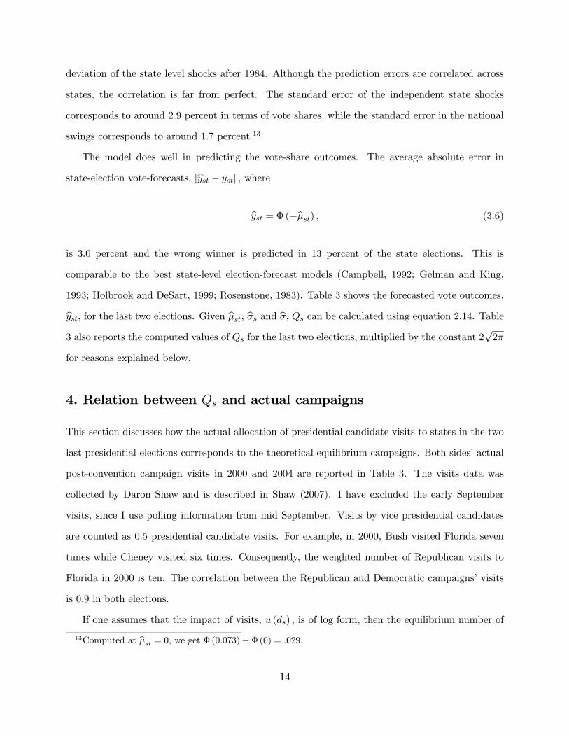
To investigate this guess, one million electoral vote outcomes were simulated for the elections

in 2000 and 2004, by using the predicted state-preference means, and drawing state and national

popularity-shocks from their estimated distributions.16 Then, the share of elections where a state

was decisive in the Electoral College and at the same time had a state election outcome between 49

and 51 percent was recorded. The results are reported in Table 3, in the columns labelled Decisive

swing st. These simulated probabilities should roughly equal to Qs, multiplied by 2√2π (Appendix

8.3 explains the scaling factor). The simple correlation between these simulated probabilities and

Qs is 0.998. This correlation is not just a picking up size. The correlation between Qs per electoral

vote and the simulated probabilities per electoral vote is still 0.998. So Qs and the probability

of being a decisive swing state are interchangeable, for practical purposes. The 0.002 difference

could result on the Qs-side from using the approximate probability of winning the election, and on

16Replace µst by the estimated bµst in equation (3.1), and draw ηst and ηt from their estimated distributions

N³0, bσ2s´ and N

³0, bσ2´, respectively to generate election outcomes yst.

22

the simulation-side from using a finite number of simulations and recording state election results

between 49 and 51 percent, whereas theoretically it should be exactly 50 percent.

Another interpretation of Qs provides a link to the literature concerning “voting power”, that

is, the probability that one vote decides the election.17 In Appendix 8.3, it is shown that

Qs ≈ (# votes cast)s * (“voting power”)s (5.2)

* (marginal voter density, conditional on tied state election)s.

This shows that candidates in a probabilistic voting model who act strategically to win the election

will allocate more resources to places with higher voting power. In contrast, the previous literature

on probabilistic voting has focused on the marginal voter density in explaining government resource

allocations (see Lindbeck andWeibull (1987), or Persson and Tabellini (2000)). This is natural since

that literature dealt primarily with direct national elections, see equation (8.20) for the equivalent

interpretation of Qs under direct elections.18

5.2. The effect of electoral votes on influence

The analytic form of Qs helps us understand why some states get more resources. A first important

observation is that Qs is roughly proportional to the number of electoral votes.19 This is evident

from the definition of Qs in equation (2.13), in combination with the fact that the first term, labelled

Qsµ, is considerably larger than the second term, Qsσ (see below). Since campaign visits seem to

be allocated proportionally to Qs, this implies that campaign resources are increasing in proportion

to the number of electoral votes.

This implies that small states are advantaged. Since all states have at least 3 electoral votes,

17See, for example, Banzaf (1968), Merrill (1978), Chamberlain and Rothschild (1988), Gelman, King andBoscardin (1998), and Gelman and Katz (2001)18However, in an extension, Lindbeck and Weibull (1987) show that candidates who maximize the proba-

bility of winning in a direct national election should spend more to voters with high "voting power" if this isheterogeneous across voters.19This result is consistent with "voting power" being proportional to the number of electoral votes. This

has been argued theoretically by Chamberlain and Rothschild (1981) and empirically by Gelman and Katz(2001). It is inconsistent with ”voting power” being more than proportional to size. Banzaf 1967, Brams andDavis (1974) find this result in the special case that each state votes for either candidate with probability1/2.

23

small states have many electoral votes per capita. At the extremes, in 2000, Wyoming had 6.1

electoral votes per capita million, and California only 1.6. For this reason, small states should get

more resources per capita. Small states are, however, disadvantaged for another reason. To see this,

one must look at the distribution of Qs per electoral vote. The following two sub-sections will, in

turn, discuss the two additively separable parts of Qs/es defined in equation (2.13):

Qs/es = Qsµ/es +Qsσ/es.

5.3. Influence per electoral vote and forecasted vote shares

The attention that states with similar number of electoral votes get depends crucially on the fore-

casted Democratic vote shares, but in a non-obvious way. This is illustrated in Figure 5.1. The

circular dots show the estimated probabilities that a state is decisive in the Electoral College and

simultaneously has a state-election outcome between 49 and 51 percent, per electoral vote. The

graph also includes a solid line plotting the values of Qsµ per electoral vote, defined in equation

(2.13). Recall that Qsµ is the part of Qs that arises because the candidates try to affect the mean

number of electoral votes. As Figure 5.1 shows, the curve accounts for most of the variation across

states. Since states like New York and Texas are far out in the tails of this curve, they were never

in a million simulated elections decisive in the Electoral College and simultaneously had a state-

election outcome between 49 and 51 percent. Consequently, the candidates can safely ignore them.

States like Florida, Michigan, Pennsylvania, and Ohio are close to the center of this distribution

and candidates should pay them frequent visits. The solid line is in fact closely approximated by a

normal distribution, multiplied by a constant, see Appendix 8.4. It can therefore be characterized

by three features: its amplitude, its mean, and its variance.

Amplitude: The amplitude denotes the general height of the distribution and is increasing in

the expected closeness of the election. It affects all states in a single election in the same way and

explains why the average probability of being a decisive swing state varies between elections. For

example, Qsµ reaches ten times higher values in 2000 than in 2004, since the former election was

24

ME MANY

PA

MI

OH

FL

TXUT WY

CA

AK

0.0

005

.001

.001

5.0

02

30 40 50 60 70Forecasted Democratic vote share

2000

ME

MARIDE

NY

PA

IL

MI

OH

KS

MO

FL

TXUTWY CA

OR

WA

0.0

0005

.000

1.0

0015

.000

2

30 40 50 60 70Forecasted Democratic vote share

2004Pr(Decisive in EC and state win margin < 2%) / electoral vote

Q / electoral votesµ

ME MANY

PA

MI

OH

FL

TXUT WY

CA

AK

0.0

005

.001

.001

5.0

02

30 40 50 60 70Forecasted Democratic vote share

2000

ME

MARIDE

NY

PA

IL

MI

OH

KS

MO

FL

TXUTWY CA

OR

WA

0.0

0005

.000

1.0

0015

.000

2

30 40 50 60 70Forecasted Democratic vote share

2004Pr(Decisive in EC and state win margin < 2%) / electoral vote

Q / electoral votesµ

Pr(Decisive in EC and state win margin < 2%) / electoral vote

Q / electoral votesµsµ

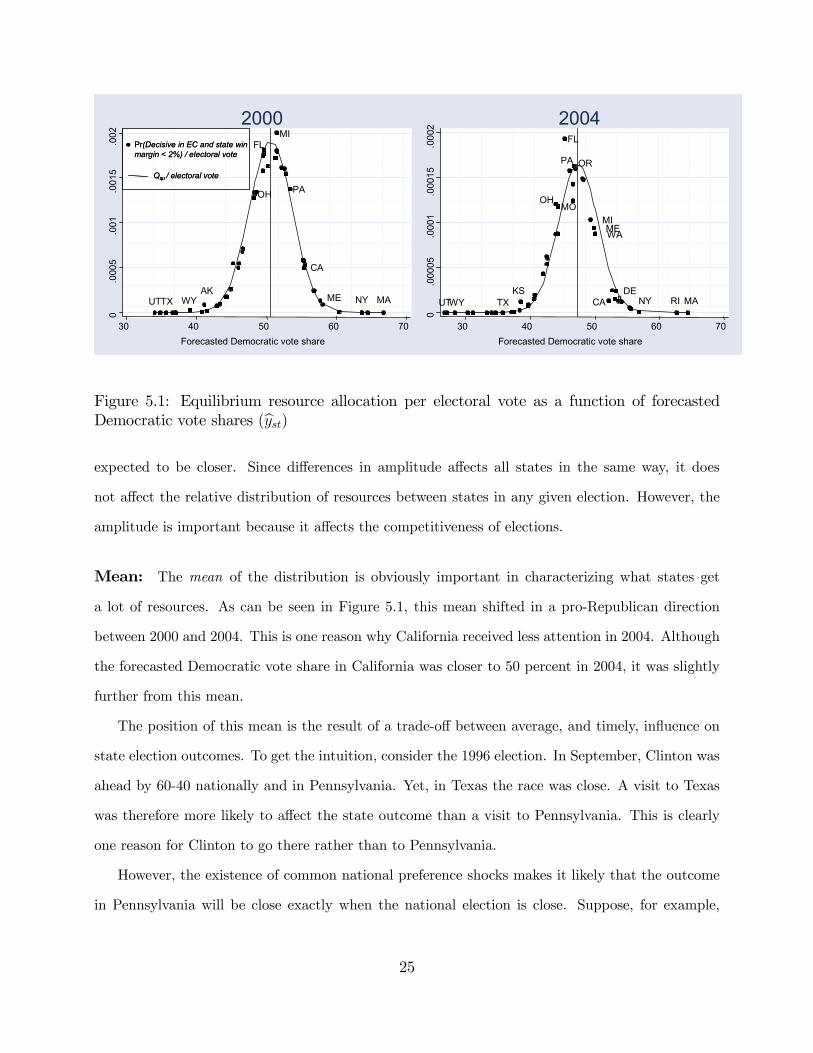
Figure 5.1: Equilibrium resource allocation per electoral vote as a function of forecastedDemocratic vote shares (byst)expected to be closer. Since differences in amplitude affects all states in the same way, it does

not affect the relative distribution of resources between states in any given election. However, the

amplitude is important because it affects the competitiveness of elections.

Mean: The mean of the distribution is obviously important in characterizing what states get

a lot of resources. As can be seen in Figure 5.1, this mean shifted in a pro-Republican direction

between 2000 and 2004. This is one reason why California received less attention in 2004. Although

the forecasted Democratic vote share in California was closer to 50 percent in 2004, it was slightly

further from this mean.

The position of this mean is the result of a trade-off between average, and timely, influence on

state election outcomes. To get the intuition, consider the 1996 election. In September, Clinton was

ahead by 60-40 nationally and in Pennsylvania. Yet, in Texas the race was close. A visit to Texas

was therefore more likely to affect the state outcome than a visit to Pennsylvania. This is clearly

one reason for Clinton to go there rather than to Pennsylvania.

However, the existence of common national preference shocks makes it likely that the outcome

in Pennsylvania will be close exactly when the national election is close. Suppose, for example,

25

that there was a sudden downturn of the national economy and that Clinton was blamed for this,

dropping his polls to 50-50 nationally. Then the situation in Pennsylvania is also likely to be 50-50

since all states were affected by the shock, while Texas would go to Dole for sure. In general, if

Texas is still a 50-50 state on election day, then chances are that Clinton is winning by a landslide,

while if Pennsylvania is a 50-50 state on election day, then it is more likely that the national election

close. Therefore, although a visit influences the outcome in Texas more frequently, it may influence

the outcome in Pennsylvania more when it matters.

More formally, note that

Qs ≈ Pr [decisive swing state] = Pr [swing state] Pr [decisive|swing state] .

The probability of being a swing state, measures the average influence on the state elections, which

is high for 50-50 states like Texas. The probability of a state’s electoral votes being decisive,

conditional on that state having a 50-50 election, is high for states like Pennsylvania. An extra visit

only matters if the state is 50-50 on election day, and the candidates must condition their visits on

this circumstance.20

The model shows how to strike a balance between average and timely influence. The less

correlated the state election outcomes, the more time should be spent in 50-50 states like Texas.21

The reason is that without national swings, the state outcomes are not correlated, and a state being

a swing state on election day carries no information about the outcomes in the other states. In my

estimates, maximum attention should typically be given to states approximately halfway between

50-50 and the forecasted national election outcome. In September of 2004, Bush was ahead by 4

percentage points. The maximum Qsµ per electoral vote was obtained for states where Bush was

expected to win by 2.5 percentage points, as illustrated in Figure 5.1. We now end the discussion

of the position of the mean, which is helpful in identifying which states will get most attention, and

look at the variance which affects the concentration of attention.20Feddersen and Pesendorfer (1996) put forward similar arguments for voters in "The Swing Voter’s Curse".21Appendix 8.3 shows this analytically.

26

0.0

005

.001

.001

5.0

02Q

smpe

r ele

ctor

al v

ote

30 40 50 60 70Forecasted Democratic vote share

State-level opinion pollNo state-level opinion polls

0.0

005

.001

.001

5.0

02Q

smpe

r ele

ctor

al v

ote

30 40 50 60 70Forecasted Democratic vote share

State-level opinion pollNo state-level opinion pollsState-level opinion pollNo state-level opinion polls

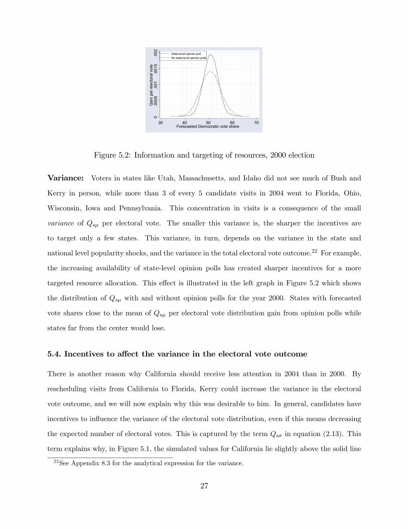
Figure 5.2: Information and targeting of resources, 2000 election

Variance: Voters in states like Utah, Massachusetts, and Idaho did not see much of Bush and

Kerry in person, while more than 3 of every 5 candidate visits in 2004 went to Florida, Ohio,

Wisconsin, Iowa and Pennsylvania. This concentration in visits is a consequence of the small

variance of Qsµ per electoral vote. The smaller this variance is, the sharper the incentives are

to target only a few states. This variance, in turn, depends on the variance in the state and

national level popularity shocks, and the variance in the total electoral vote outcome.22 For example,

the increasing availability of state-level opinion polls has created sharper incentives for a more

targeted resource allocation. This effect is illustrated in the left graph in Figure 5.2 which shows

the distribution of Qsµ with and without opinion polls for the year 2000. States with forecasted

vote shares close to the mean of Qsµ per electoral vote distribution gain from opinion polls while

states far from the center would lose.

5.4. Incentives to affect the variance in the electoral vote outcome

There is another reason why California should receive less attention in 2004 than in 2000. By

rescheduling visits from California to Florida, Kerry could increase the variance in the electoral

vote outcome, and we will now explain why this was desirable to him. In general, candidates have

incentives to influence the variance of the electoral vote distribution, even if this means decreasing

the expected number of electoral votes. This is captured by the term Qsσ in equation (2.13). This

term explains why, in Figure 5.1, the simulated values for California lie slightly above the solid line

22See Appendix 8.3 for the analytical expression for the variance.

27

in 2000 and considerably below the line in 2004. (In general, why in this figure, states close to the

right of the mean lie above the curve in 2000, while states close to the left lie below. In 2004, the

situation is the reverse.)

To get the intuition of why such behavior is rational, consider the following example from the

world of ice hockey. One team is trailing by one goal and there is only one minute left of the

game. To increase the probability of scoring an equalizer, the trailing team pulls out the goalie and

puts in an extra offensive player. Most frequently, the result is that the leading team scores. But

the trailing team does not care about this, since they are losing the game anyway; they only care

about increasing the probability that they score an equalizing goal, which is higher with an extra

offensive player. Therefore, it is better to increase the variance in goals, even though this decreases

net expected goals. In contrast, if they were allowed, the leading team would like to pull out an

offensive player and put in an extra goalie.

Similarly, a presidential candidate who is behind should try to increase variance in the election

outcome. He can do this by spending more time in large states where he is behind (putting in an

extra offensive player), and less time in states where he is ahead (pulling the goalie). A candidate

who is ahead should instead try to decrease variance in electoral votes, thus securing his lead, by

spending more time in large states where he is ahead (putting in an extra goalie), and less time in

states where he is behind (pulling out an offensive player). Both candidates thus spend more time

in large states where the expected winner is leading.

To formally see why a trailing candidate increases the variance by spending more time in states

with many electoral votes where he is behind, consider equation (2.8) showing the variance, condi-

tional on a national shock. The variance in the number of electoral votes from a state is proportional

to these votes squared. Therefore, the effect on the total variance, per electoral vote, is larger in

large states. Further, the variance in a state outcome is higher the closer the expected result is to

a tie. By visiting a state where the leading candidate is ahead, the trailing candidate moves the

expected result closer to a tie, and increases the variance in election outcome. Similarly, decreasing

the number of visits to a state where the lagging candidate is leading increases the variance

Figure 5.3 illustrates this effect by plotting the values of the analytical expression for Qsσ per

28

PA

MI

OH

CA

-.000

1-.0

0005

0.0

0005

.000

1.0

0015

30 40 50 60 70Forecasted Democratic vote share

2000

ILMI

OH

FL

CA-.000

1-.0

0005

0.0

0005

.000

1

30 40 50 60 70Forecasted Democratic vote share

2004

Figure 5.3: Incentives to influence variance

electoral vote. In 2004, the lagging candidate (Kerry) should put in extra offensive visits in states

like Florida and Ohio, at the cost of weakening the defense of states like California and Illinois.

The leading candidate (Bush) should defend his lead in states like Florida and Ohio, at the cost

of not challenging Kerry’s lead in California and Illinois. This resounds with the result by Snyder

(1989) that parties will spend more in safe districts of the advantaged party than in safe districts

of disadvantaged party.

5.5. Additional issues

Finally, we discuss how results would be affected by the inclusion of minority candidates, by the fact

that the electoral votes of Maine and Nebraska are allocated in a special fashion and if campaigns

affect turnout rather than vote choice. Starting with the last issue, if the campaigns affected turnout,

more resources should still be devoted to states likely to be decisive swing states. Only in decisive

swing states can a marginal increase in turnout among own-party supporters change the national

election outcome. A difference would be that the marginal voter density would be replaced by the

marginal-turnout density measuring how easily supporters in a state can be mobilized from the pool

of non-voters.23

In terms of this model, minority candidates will matter through their effect on the two-party

23For a model of turnout in presidential elections, see Shachar and Nalebuff (1999).

29

preference distributions in the states. Suppose that it is known when campaign plans are made

that the minority candidate runs, and the state and national polls take this into account. Then the

effect of the minority candidate is taken into account in computing the probability that each state

is a decisive swing state and the equilibrium is unaffected. If there is uncertainty about whether the

candidate will run, then the model should be amended to account for this additional uncertainty.

It is more difficult to include the specific procedure of allocating electoral votes in Maine and

Nebraska into the model. The model can easily be extended to account for the electoral votes

that are allocated in the congressional district elections. However, it is harder to incorporate the

2 electoral votes that are allocated in proportion to the state election. For the 2000 election, this

does probably not have a large impact since Nebraska was solidly Republican and Maine solidly

Democratic, but in 2004, Maine was less clearly Democratic and the allocations would perhaps be

affected.

6. Electoral reform

Since the Electoral College creates very sharp incentives to target only a few states, a natural

question to ask is whether there are other ways of electing president that would make candidates

care more equally for all voters. Hence, we now analyze candidate visits under a direct national

popular vote system (Direct Vote), the reform that has come closest to being accepted.24 We also

discuss the effects of keeping the electoral college, but having electoral votes allocated proportionally

to the popular votes in the states (the Lodge-Gossett Amendment).25 We focus on the distribution

of visits: which states gains or loses from reform, and what electoral system creates a more unequal

visit schedule. However, the model is also used to evaluate and quantify how reform impacts

attention to minorities, and the expected frequency of razor-thin victories and presidents without

a majority of the popular vote.

First, we develop the model for Direct Vote. Suppose the president is elected by a direct national

vote. The number of Democratic votes in state s is then equal to the number of voters in the state,

24A Direct Vote reform was proposed by House Representative Emanuel Celler in 1969. It was wildlypopular in the House, passing 338-70, but failed to pass in the Senate due to a filibuster.25This amendment passed the Senate by a vote of 64-27, but was rejected in the House.

30

vs, multiplied by the Democratic vote-share, ys. The Democratic candidate wins the election if he

receives more than half of the popular votes in the nation:

Xs

vsys ≥1

2

Xs

vs. (6.1)

Using again the Central Limit Theorem of Liapounov, the number of votes won by candidate D is

asymptotically normally distributed with mean and variance,

µv =Xs

vsΦ

⎛⎝∆us − µs − ηqσ2s + σ2fs

⎞⎠ , (6.2)

σ2v = σ2v (∆us, η) .

See Appendix 8.5 for the explicit expression for σ2v. The probability of a Democratic victory is

PD = 1−ZΦ

Ã12

Ps vs − µvσv

!dη.

As before, both candidates choose the number of days to visit each state, subject to the constraint

on the total number of days left in equation (2.1). The following proposition characterizes the

equilibrium allocation.

Proposition 3. A pair of strategies for the parties¡dD, dR

¢that constitute a NE in the game of

maximizing the expected probability of winning the election must satisfy dD = dR = d∗, and for all

s and for some λ > 0

QDVs u0 (ds) = λ. (6.3)

The interpretation of QDVs is (see Appendix 8.5.),

QDVs ≈ (# votes cast)s * (“voting power”) (6.4)

* (marginal voter density, conditional on tied national election)s.

However, “voting power” is now the same for all voters, since any voter is decisive if and only if

31

the election is won by no more than one vote. Hence, QDVs varies across states only because of

differences in the share of marginal voters and the number of voters.

The allocation under Direct Vote depends crucially on the share of marginal voters, which

in turn depends on the estimated variance in the preference distribution, σ2fs. Therefore, the

restriction σfs = 1 is removed in the maximum likelihood estimation of equation (3.2), as well as

the assumption that σs is the same for all states. (To make the results comparable, the Qs relevant

for the Electoral College system is re-estimated with the same restrictions removed.) The model

identifies σfs through the response in vote shares to changes that are common to all states, and

observable changes in economic growth at national and state level, incumbency variables, home state

of the president and vice president. States where vote shares co-vary strongly with these variables

are estimated to have many marginal voters. Rhode Island is estimated to have the largest share

of marginal voters and Mississippi the smallest.

6.1. Distribution of visits

We can now identify states that would have gained or lost candidate attention from reform. Figure

6.1 shows the 1948-2000 averages of equilibrium number of visits per capita, relative to the national

averages, under both systems, assuming that u (ds) is of log form.26 States above 1 on the y-axis

receive more than average visits per capita under the Electoral College system, whereas states to

the right of 1 on the x-axis have more visits per capita than average under the Direct Vote system.

Thus states below the 45-degree line would have gained from reform, those above would have

lost. Some states, like Maine and New Hampshire, are well off under both systems while Mississippi

is disadvantaged under both. Other states, like Nevada are among the winners in the present system

but among the losers under Direct Vote. The opposite is true for Rhode Island and Kansas.

States gain or lose attention because of their (i) electoral size per capita and (ii) influence

26The graph showsQs

ns1n

PQs

,

where upper bar denotes 1948-2004 averages.

32

CTME

MA

NH

RI

VT

DE

NJ

NY

PAIL

IN

MI

OHWI

IA

KS

MNMO

NE

ND

SD

VA

AL

ARFL

GA

LA

MSNC

SCTX

KYMD

OKTN

WV

AZ

COID

MTNV

NM

UT

WY

CA

OR

WA

AK

HI

01

23

4E

lect

oral

Col

lege

0 .5 1 1.5 2Direct Vote

Visits per capita

Figure 6.1: Equilibrium visits per capita and advertisements, relative to national average

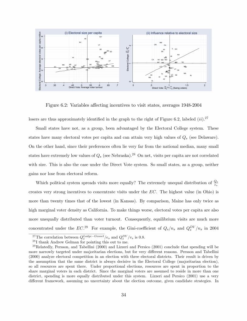
relative to electoral size. Under the two systems, these components are

(i) (ii)

EC : Qs

ns= es

nsQs

es

DV : QDVsns

= vsns

QDVsvs

.

Figure 6.2 plots the 1948-2004 averages of these components. For example, the Figure to the right

shows why Rhode Island and Massachusetts would gain from reform. Because of their average

partisanship, these states are rarely competitive when the national election is close. Consequently,

they do not receive much attention under the Electoral College system. Still, these states have quite

a few marginal (swing) voters, making them attractive targets under Direct Vote. In the Figure to

the left, we see that Nevada and Delaware would get less attention after reform primarily because

of their heavy endowment of electoral votes relative to popular votes.

We can now also identify states that would gain attention under the Lodge-Gossett Amendment.

This suggested keeping the electoral size per capita (i) constant, while only changing the influence

per electoral size (ii) from that induced by a state-level winner-takes-all system to a state-level

proportional system. In the latter system, marginal voter densities matter, and the winners and

33

SCGA

MSVATX

ALAR

LA

HI

TNNCFL

AZ

NV

MDKY

AK

CA

NM

NY

OK

PA NJ

NE

OH

KS

WA

WV

CO

MI

VT

MO

RI

IN

DE

WY

OR

IL

ME

MA

IDNH

CT

MT

WIIA

ND

UT

SD

MN

02

46

8E

lect

oral

Col

lege

: Ave

rage

ele

ctor

al v

otes

per

cap

ita m

illion

.3 .35 .4 .45 .5 .55 .6 .65 .7Direct Vote: Average voter turnout

(i) Electoral size per capita

AL

AK

AZ

AR

CA

CO

CT

DE

FL

GAHI

ID

IL

IN

IA

KS

KYLA ME

MD

MA

MI

MN

MS

MO

MT

NE

NV

NH

NJ

NM

NY

NCND

OH

OK

OR PA

RISC

SD

TN

TX UT

VT

VA

WA

WV

WI

WY

01

2E

lect

oral

Col

lege

: Qs/

e s

0 .5 1 1.5 2Direct Vote: Qs

DV/ vs (Swing voters)

(ii) Influence relative to electoral size

SCGA

MSVATX

ALAR

LA

HI

TNNCFL

AZ

NV

MDKY

AK

CA

NM

NY

OK

PA NJ

NE

OH

KS

WA

WV

CO

MI

VT

MO

RI

IN

DE

WY

OR

IL

ME

MA

IDNH

CT

MT

WIIA

ND

UT

SD

MN

02

46

8E

lect

oral

Col

lege

: Ave

rage

ele

ctor

al v

otes

per

cap

ita m

illion

.3 .35 .4 .45 .5 .55 .6 .65 .7Direct Vote: Average voter turnout

(i) Electoral size per capita

AL

AK

AZ

AR

CA

CO

CT

DE

FL

GAHI

ID

IL

IN

IA

KS

KYLA ME

MD

MA

MI

MN

MS

MO

MT

NE

NV

NH

NJ

NM

NY

NCND

OH

OK

OR PA

RISC

SD

TN

TX UT

VT

VA

WA

WV

WI

WY

01

2E

lect

oral

Col

lege

: Qs/

e s

0 .5 1 1.5 2Direct Vote: Qs

DV/ vs (Swing voters)

(ii) Influence relative to electoral size

Figure 6.2: Variables affecting incentives to visit states, averages 1948-2004

losers are thus approximately identified in the graph to the right of Figure 6.2, labeled (ii).27

Small states have not, as a group, been advantaged by the Electoral College system. These

states have many electoral votes per capita and can attain very high values of Qs (see Delaware).

On the other hand, since their preferences often lie very far from the national median, many small

states have extremely low values of Qs (see Nebraska).28 On net, visits per capita are not correlated

with size. This is also the case under the Direct Vote system. So small states, as a group, neither

gains nor lose from electoral reform.

Which political system spreads visits more equally? The extremely unequal distribution of Qs

es

creates very strong incentives to concentrate visits under the EC. The highest value (in Ohio) is

more than twenty times that of the lowest (in Kansas). By comparison, Maine has only twice as

high marginal voter density as California. To make things worse, electoral votes per capita are also

more unequally distributed than voter turnout. Consequently, equilibrium visits are much more

concentrated under the EC.29 For example, the Gini-coefficient of Qs/ns and QDVs /ns in 2004

27The correlation between QLodge−Gossets /es and QDV

s /vs is 0.8.28I thank Andrew Gelman for pointing this out to me.29Relatedly, Persson, and Tabellini (2000) and Lizzeri and Persico (2001) conclude that spending will be

more narrowly targeted under majoritarian elections, but for very different reasons. Persson and Tabellini(2000) analyze electoral competition in an election with three electoral districts. Their result is driven bythe assumption that the same district is always decisive in the Electoral College (majoritarian election),so all resources are spent there. Under proportional elections, resources are spent in proportion to theshare marginal voters in each district. Since the marginal voters are assumed to reside in more than onedistrict, spending is more equally distributed under this system. Lizzeri and Persico (2001) use a verydifferent framework, assuming no uncertainty about the election outcome, given candidate strategies. In

34

were 0.73 and 0.17, respectively. The equilibrium TV-advertisements across media markets are also

more unequally distributed under the Electoral College system than under Direct Vote. In 2004,

the Gini-coefficient of equilibrium advertisements (Qm/pm) across media markets was 0.70 under

the Electoral College compared to 0.13 under Direct Vote.

6.2. Other reform concerns

A frequent claim is that minorities are concentrated in large, politically competitive states and thus

have higher than average influence on the election.30 However, this seems inconsistent with the data

on advertisements across 75 media markets in 2000 discussed in Section 4. In fact, a randomly drawn

Hispanic voter had 21 percent fewer ads aired in his media market in 2000 than the average voter.

The equivalent number for African Americans was 11 percent fewer ads. Since the model predicts

advertisements well, we reach virtually the same results using the model-predicted equilibrium

advertisements across these markets in 2000 (20 and 9 percent, respectively). Model-predicted

advertisements for all media markets and elections after 1980 indicate that these differences are

recent for Hispanics,31 but long term for African Americans. On average, 1980-2004, there was no

difference between Hispanics and the average voter, while a randomly drawn African voter had 8

percent fewer predicted ads aired in his media market than the average voter. This is perhaps not

surprising, given that the greatest concentration of African Americans are found in Washington

D.C. and the Deep South states.

Often discussed concerns are presidents without a majority of the popular vote and razor-thin

victories. Since these are very rare events, it is hard to estimate their probabilities using empirical

frequencies. However, given that the elections 1948-2004 are representative of future elections,

these probabilities can be estimated by using the model to simulate elections and recording event

each particular election, spending will be targeted to half of the voters in half of the states under theElectoral College system, and half of the voters in the nation under Direct Vote. Therefore, resources arespent in a more concentrated fashion under the Electoral College system. Since candidates use completelymixed strategies, over time all states receive equal expected treatment.30See Kimberling, William C., 2005, "The Electoral College", Federal Election Commission Office of Elec-

tion Administration, www.fec.gov/pdf/eleccoll.pdf., Kristina Dell, "The Electoral College Explained", TimeMagazine, Nov. 1, 2004; or Alexander Keyssar in "Pro’s & Cons: The Electoral College", The JournalEditorial Report, Oct. 29, 2004.31I could not find county-level data on Hispanic population prior to 1980.

35

frequencies. The estimated probability of a winning margin less than 1000 votes is about 40 times

higher under the Electoral College system (0.8 percent compared to 0.02 percent under Direct

Vote). The estimated probability of electing a president without a majority of the popular vote is

about four percent. This implies that we should expect this outcome about once in every hundred

years. Historically, it has happened around three (perhaps four) times in the last 200 years: 1824

(perhaps), 1876, 1888, and 2000. Arguably, however, the outcomes in 1824 and 1876 had to do with

peculiarities in the aggregation of votes.32

7. Conclusion and discussion

This paper develops a probabilistic-voting model of electoral competition under Electoral College

system of electing president. The modeling framework is significantly more general than previous

work — with S states, a varying number of electoral votes per state, preference distributions varying

across states, uncertainty regarding the election outcome at both state and national level, etc. —

which allows a fairly direct application to the election incentives facing a U.S. presidential candidate

or incumbent president. In addition, the model can be explicitly solved and directly estimated. This

implies that new questions can be asked and a new type of answers be given.

Some theoretical results deserve mentioning. First, more resources should be devoted to states

who are likely to be decisive swing states, that is, states who are decisive in the electoral college and,

at the same time, have tied state elections. Second, the probability of being a decisive swing state

equals the number of voters in the state multiplied by the “voting power” in the state, multiplied

by the marginal voter density conditional on the state election being tied. Third, the probability

of being a decisive swing state is roughly proportional to the number of electoral votes. Fourth,

this probability per electoral vote is highest for states who have a forecasted state election outcome

that lies between a draw and the forecasted national election outcome. Fifth, more precise state-

election forecasts make the optimal allocation of resources more concentrated. Sixth, the presidential

32In 1824, six of the twenty four States at the time still chose their Electors in the State legislature, so thepopular vote outcome is not known. In the chaotic election of 1876, each State delivered to Congress twoslates of electors and a special commission accepted slates favoring of the popular vote loser. See "A BriefHistory of the Electoral College" in http://www.fec.gov/elections.html.

36

candidate who is lagging behind should try to increase the variance in electoral votes. This can

be achieved by spending more time in large states where this candidate is behind, and less time in

large states where this candidate is ahead.33

Most importantly, this paper quantifies these effects. This makes it possible to identify which

states have been benefiting from the Electoral College system. It also reveals a very close resem-

blance between the presidential candidates’ actual strategies and the equilibrium strategies in the

last two elections. Finally, it shows the sharp incentives to favor certain states created by the

Electoral College system.

This paper also analyzes the effects of a change to direct national popular vote for president.

Different factors guide attention under the two electoral systems: voter turnout and the share swing

voters under Direct Vote; and the probability of being a decisive swing state under the Electoral

College. These factors determine what states are likely to gain or lose candidate attention after

reform; see Figure 6.1. Since the probability of being a decisive swing state is much more unequally

distributed than the other factors, the Electoral College system induces presidential candidates to

pay less equal attention to states than Direct Vote. Finally, neither small states nor minorities have

been favored by the Electoral College system.

The model of this paper can be applied both to resources solely used in the campaign, such as

visits, and to campaign promises with policy consequences. This has two important implications.

First, the above theoretical results also apply to policy incentives (but, of course, we do not yet

know how empirically important these are). For example, the Electoral College system provides

sharper incentives to target a few states with favorable policies, and Figure 6.1 shows how incentives

to offer favorable policies would change after reform.

Second, a general lesson is that while analyzing campaigning is most interesting in its own right,

it is also a useful step to learn about electoral incentives to distort policy. Pure campaign efforts

33The second, fourth and fifth points are new, to the best of my knowledge. The first point shows moreprecisely what people have conjectured or partly demonstrated earlier; see, for example, Snyder (1989). Thethird point has not previously been shown theoretically, although (because of the second point) it is closelyrelated to the empirical finding of Gelman and Katz (2001) that "voting power" is proportional to size underreasonable assumptions. The sixth point makes more precise the statement of Snyder (1989) that moreresources will be spent in safe districts of the advantaged party than in the safe districts of the other party.

37

are only used to win elections and very informative of how politicians perceive electoral incentives.

Policy is determined by a multitude of factors, of which election concerns is one. For this reason, a

cautious approach is to first test models of political competition on campaigning, and then proceed

to test for this signal also in policy. This paper takes the first step and leaves the second to future

research.

This paper contributes to the literature on the comparative political economy that links political

institutions to outcomes in politics and economic policy. However, the paper is slightly methodolog-

ically different since the model is sufficiently rich to allow the complete integration of theory and

empirics, tying together theoretical insights with empirical results. Since the modeling framework is

quite general, this integration can be carried over to the study of other resource allocation problems

in other electoral settings.

38

References

[1] Banzhaf, John R., 1968, ”One Man, 3.312 Votes: A Mathematical Analysis of the Electoral

College”, Villanova Law Review 13, 304-332.

[2] Brams, Steven J. and Morton D. Davis, 1974, ”The 3/2 Rule in Presidential Campaigning.”

American Political Science Review, 68(1), 113-34.

[3] Besley, Timothy

[4] Besley, Timothy and Anne Case, "Political Institutions and Policy Choices: Evidence from the

United States", Journal of Economic Literature, March 2003, 41(1), 7-73.

[5] Campbell, James E., 1992, Forecasting the Presidential Vote in the States. American Journal

of Political Science, 36, 386-407.

[6] Chamberlain, Gary and Michael Rothchild, 1981, ”A Note on the Probability of Casting a

Decisive Vote”, Journal of Economic Theory 25, 152-162.

[7] Colantoni, Claude S., Terrence J. Levesque, and Peter C. Ordeshook, ”Campaign resource

allocation under the electoral college (with discussion)”, American Political Science Review 69,

1975, 141-161.

[8] Feddersen, Timothy J. and Wolfgang Pesendorfer, 1996. "The Swing Voter’s Curse," American

Economic Review, vol. 86(3), 408-24.

[9] Gelman, Andrew, and Jonathan N. Katz, 2001, ”How Much Does a Vote Count? Voting Power,

Coalitions, and the Electoral College”, Social Science Working Paper 1121, California Institute

of Technology.

[10] Gelman, Andrew, and Gary King, 1993, ”Why are American Presidential Election Campaign

Polls so Variable when Votes are so Predictable?”, British Journal of Political Science, 23,

409-451.

39

[11] Gelman, Andrew, Gary King, and W. John Boscardin, 1998, ”Estimating the Probability

of Events that have Never Occurred: when is your vote decisive?”, Journal of the American

Statistical Association, 93(441), 1-9.

[12] Hobrook, Thomas M. and Jay A. DeSart, 1999, ”Using State Polls to Forecast Presidential

Election Outcomes in the American States”, International Journal of Forecasting, 15, 137-142.

[13] Kimberling, William C., "The Electoral College", mimeo, Federal Elections Commission,

http://www.fec.gov/pdf/eleccoll.pdf

[14] Lindbeck, Assar and Jörgen W. Weibull, 1987, ”Balanced-Budget Redistribution as the Out-

come of Political Competition”, Public Choice, 52, 273-97.

[15] Lizzeri, Allesandro and Nicola Persico, 2001, "The Provision of Public Goods under Alternative

Electoral Incentives", American Economic Review, 91(1), 225-239.

[16] Merrill, Samuel III, 1978, ”Citizen Voting Power Under the Electoral College: A Stochastic

Voting Model Based on State Voting Patterns”, SIAM Journal on Applied Mathematics, 34(2),

376-390.

[17] Milesi-Ferretti, Gian Maria, Perotti, Roberto, and Rostagno, Massimo, 2002, “Electoral Sys-

tems and Public Spending,” The Quarterly Journal of Economics 117, 609-657.

[18] Morton, Rebecca B., ”Analyzing Elections”, Norton, forthcoming. Presently available at

http://www.nyu.edu/gsas/dept/politics/faculty/morton/morton_book.html.

[19] Persson, Torsten and Guido Tabellini, 1999, ”The Size and Scope of Government: Comparative

Politics with Rational Politicians,” European Economic Review 43, 699-735.

[20] Persson, Torsten, and Guido Tabellini, 2000, Political Economics: Explaining Economic Policy,

MIT Press.

[21] Ramanathan, Ramu, 1993, "Statistical Methods in Econometrics", San Diego: Academic Press.

[22] Rosenstone, Steven J., 1983, ”Forecasting Presidential Elections”, New Haven: Yale University

Press.

40

[23] Shachar, Ron and Barry Nalebuff, 1999, ”Follow the Leader: Theory and Evidence on Political

Participation”, American Economic Review 89(3), 525-547.

[24] Shaw, Daron R., "The Race to 270", Chicago: University of Chicago Press, 2007.

[25] Strömberg, David, 2002, ”Optimal Campaigning in Presidential Elections: The Probability of

Being Florida”, IIES working paper 706.

[26] Snyder, James M., 1989, ”Election Goals and the Allocation of Campaign Resources”, Econo-

metrica 57(3), 637-660.

41

8. Appendix

8.1. Proof of Proposition 1

Since PD¡dD∗, dR

¢is continuous and differentiable, a necessary condition for an interior NE is

∂PD¡dD∗, dR∗

¢∂dDs

= Qsu0 ¡dD∗s ¢

= λD, (8.1)

∂PD¡dD∗, dR∗

¢∂dRs

= Qsu0 ¡dR∗s ¢ = λR. (8.2)

Therefore,u0¡dD∗s

¢u0 (dR∗s )

=λD

λR, (8.3)

for all s. Suppose that dD∗ 6= dR∗. This means that dD∗s < dR∗s for some s, implying that λD > λR

by equation (8.3). Because of the budget constraint, it must be the case that dD∗s0 > dR∗s0 for some

s0, which implies λD < λR, a contradiction. Therefore, λD = λR, which implies dD∗s = dR∗s for all s.

Uniqueness: Suppose there are two equilibria with equilibrium strategies d and d0 corresponding

to λ > λ0. The condition on the Lagrange multipliers implies ds > d0s for all s, which violates the

budget constraint. Therefore, the only possibility is λ = λ0, which implies ds = d0s for all s.

8.2. Data: variable definitions and sources, and sample

Tables A1 and A2 here.

8.3. Analytical interpretation of Qs

We now show analytically why Qs approximates the joint probability of a state being decisive in

the electoral college at the same time as having a close election. First, an expression for the approx-

imate probability that a particular state, denoted s0, is decisive in the electoral college is derived.

Disregarding s0, the electoral vote outcome,P

s6=s0 Dses, is approximately normally distributed with

mean

µ−s0 = µ− esGs (·) (8.4)

42

and variance

σ2E−s0 = σ2E − e2sGs (·) (1−Gs (·)) . (8.5)

The es0 electoral votes of state s0 are decisive if

Xs6=s0

Dses ∈µP

s 6=s es

2,

Ps6=s es

2− es0

¶.

In this range, a presidential candidate wins if and only if he receives the votes of state s0. The

probability of this event is approximately

P = Φ

Ãs es2 − µ−s0

σE−s0

!− Φ

Ãs es2 − es − µ−s0

σE−s0

!.

Inserting for µ−s0 and σ2E−s0 yields

Φ

Ãs vs2 − µ+ es0Gs0 (·)

σE−s0

!− Φ

Ãs vs2 − µ− es0 (1−Gs0 (·))

σE−s0

!.

Making a second-order Taylor-approximation of P around the point

x0 =s es2 − µ

σE−s0,

we get

P (η) ≈ ϕ (x0)es

σE−s0+

e2sσ2E−s0

ϕ (x0)x0

µGs (·)−

1

2

¶.

Given the large number of states, σE−s0 ≈ σE, implying

P (η) ≈ ϕ (x (η))esσE

+e2sσ2E

ϕ (x (η))x (η)

µGs (·)−

1

2

¶.

Second, we derive the analytical likelihood that a the election in state s0 is tied. Given a national

shock, η, the state outcome is a tie if Fs(−ηs− η) = 12 which happens with likelihood gs (−µs − η) .

Conditional on the national shock, the joint likelihood of being decisive in the electoral college and

43

having a tied election is thus roughly P (η) gs (−µs − η), and the unconditional likelihood equals

ZP (η) gs (−µs − η)h (η) dη = Qs,

by the definition of Qs in equation 2.13. Consequently, Qs approximates the joint likelihood that a

state is decisive in the electoral college and, simultaneously, has a tied state election.

To compare Qs with simulated frequencies of being EC decisive and having a state election

margin of less than two percent, Qs must be scaled. The probability of a winning margin of less

than x percent equals1

2− x

200≤ Fs(−ηs − η) ≤ 1

2+

x

200.

The probability that the state-level shock falls in this region is approximately

gs (−µs − η)σfsϕ (0)

x

100.

The unconditional probability of being pivotal and having a state-election margin of x percent is

therefore approximately

Qsσfsϕ (0)

x

100.34

The scaled values of Qs are very similar to the simulated frequencies of the corresponding

events. Table 3 reports the scaled Qs and simulated frequencies. In 4.5 percent of the 1 million

simulated elections, Florida was decisive in the Electoral College and had a state margin of victory

of less than 2 percent. The scaled Qs for Florida was 4.6 percent. To get the probability that

the state margin of victory is within, say 1000, votes, Qs should be scaled by 1000vs

σfsϕ(0) . Using this

formula, the probability of a state being decisive in the Electoral College, and at the same time

34Although the marginal voter density plays no role in Qs, it enters if Qs is re-written as

Qs ≈ Qs

µσfsϕ (0)

2

100

¶| {z }

Pr(decisive in electoral collegeand state election outcome within two percent)

ϕ (0)

σfs| {z }marginal voter density,

conditional on tied state election

100

2.

Since σfs = 1 in this part of the paper,σfsϕ(0)

2100 =

√2π 2

100 = 0.05013, is just a constant scaling factor.

44

having an election result with a state margin of victory less than 1000 was 0.0004 in Florida in the

2000 election. The probability that this would happen in any state was 1 percent. The probability

of a victory margin of one vote in Florida is 0.4 per million. The state where one vote is most likely

to be decisive is Delaware, where it is decisive .9 times in a million elections.

This type of scaling also helps to clarify the relation between Qs and “voting power”, i.e. the

probability that one vote in state s decides the election. With continuous vote outcomes, “voting

power” can be defined as the probability that the margin of victory is no more than one vote; see

Chamberlain and Rothschild (1981). Rewriting Qs, as follows

Qs ≈ vs|{z}# votes cast

in state s

Qs

µσfsϕ (0)

1

vs

¶| {z }

“voting

power”

ϕ (0)

σfs| {z },marginal voter density,

conditional on tied state election

(8.6)

shows that Qs equals the product of the number of votes cast in state, the voting power in the state,

and the marginal voter density conditional on a tied state election.

8.4. The mean and variance of the Qsµ/es distribution

This appendix will discuss the mean and variance in the distribution of Qsµ per electoral vote.

First, we will show that a simpler functional form closely approximates Qsµ. Then the properties

of this simpler function will be discussed.

To simplify the analytical form of Qsµ, we do a first-order Taylor-expansion of the mean of the

expected number of electoral votes µ (η) around η = eη for whichµ (eη) = 1

2

Xs

es, (8.7)

that is, the value of the national shock which makes the expected outcome a draw. With this

approximation,

µ (η) =Xs

esGs (−µs − η) ≈ 12

Xs

es − a (η − eη) , (8.8)

45

where

a =Xs

esgs (−µs − eη) . (8.9)

Since the mean of the electoral votes, µ (η) , is much more sensitive to national shocks than is the

variance σE (η), the latter is approximated by

σ2E (η) ≈ σ2E =Xs

e2sGs (−µs − eη) (1−Gs (−µs − eη)) . (8.10)

Using these approximations,

1

σE (η)ϕ

Ã12

Ps es − µ

σE (η)

!≈ 1

σEϕ

µη − eησE/a

¶. (8.11)

Inserting this into the definition of Qsµ in equation 2.13 we have,

Qsµ/es ≈1

σE

Zϕ

µη − eησE/a

¶gs (−µs − η)h (η) dη.

Integrating over η and simplifying,

Qsµ/es ≈1

2πqa2σ2σ2s + σ2Eσ

2s + σ2Eσ

2exp

Ã−12

à eη2σ2 + (σE/a)

2 +(µs − µ∗)2eσ2

!!, (8.12)

where

µ∗ = − σ2

σ2 + (σE/a)2eη, (8.13)

and

eσ2 = σ2s +1³

1σ2 +

1(σE/a)

2

´ . (8.14)

The above approximation is quite good. The correlation between Qsµ/es and the right hand side

of equation (8.12) is 0.9999 for observations 1948-2004.

From equation 8.12, it is clear that the amplitude of Qsµ is larger when eη is close to zero. Thisaffects all states in the same way in a particular election, but varies across elections.

The mean µ∗ of the distribution always lies between a pro-Republican state bias of µst = 0,

46

which corresponds to a 50% forecasted Democratic vote share, and µst = −eηt, which approximatelycorresponds to the forecasted national Democratic vote share. The smaller the variance of the

national popularity-swings, σ2, the closer is the mean to 50-50. (Note that σE , a, and eη do notdepend on σ2.) In the extreme case where σ2 approaches zero, then µ∗s approaches 0. In the

extreme case that σ2 approaches infinity, µ∗s approaches −eη.The smaller the variance eσ2, the larger incentives to treat states differently. Comparing two

states s and t, the ratio

Qsµ/esQtµ/et

= exp

Ã−12

Ã(µs − µ∗)2 − (µt − µ∗)2eσ2

!!,

depends on how far the two states are from µ∗s, and on eσ2.35 By the definition of eσ2 above, it isclear that eσ2 is increasing in σ2. It is also increasing in σ2s, both directly and because increases

in σ2s are associated with increases in (σE/a)2 . The latter is true in the sample and intuitive, the

larger the state-level shocks, the more uncertainty about the aggregate outcome. However, due to

effects through a it is hard to prove formally.

8.5. Direct presidential vote

First, the approximate probability of winning the election is derived under DV . Conditional on η,

the expected vote share of D in state s is

µvs (∆us, η) =

ZFs(∆us − η − ηs)gs (ηs) dηs

= Φ

⎛⎝∆us − η − µsqσ2s + σ2fs

⎞⎠ ,

and the expected national vote of D is

µv (∆us, η) =Xs

vsµvs (∆us, η) .

35As in the estimation in section 3, we assume that σ2s = σ2t .

47

Again conditional on η, the variance in D’s votes in state s is,

σ2vs = v2s

Z(Fs (∆us − η − ηs)− µvs (∆us, η))

2 gs (ηs) dηs,

and the variance in the national votes of D is

σ2v =Xs

σ2vs.

The approximate probability of D winning the election is

PD (∆us) = 1−ZΦ

Ã12

Ps vs − µvσv

!h (η) dη.

The equilibrium strategies of Proposition 3 depend crucially on

∂PD

∂∆us= QDV

s =∂PD

∂µv

∂µv∂∆us

+∂PD

∂σv

∂σv∂∆us

= QDVsµ +QDV

sσ ,

where

QDVsµ =

vs

σvqσ2s + σ2fs

Zϕ

Ã12

Ps vs − µvσv

!ϕ

⎛⎝∆us − µs − ηqσ2s + σ2fs

⎞⎠h (η) dη, (8.15)

QDVsσ =

Z ̶

∂σvΦ

Ã12

Ps vs − µvσv

!!∂σv∂∆us

h (η) dη.

8.6. Analytical interpretation of QDVsµ

Empirically, QDVsµ À QDV

sσ , the size of QDVsσ is negligible compared to QDV

sµ . The interpretation of

QDVsµ is

QDVsµ = vs (pdf of tied election) E [fs | election tied] . (8.16)

This follows since, conditional on η, the expected marginal voter density in state s is

Z ∞

−∞fs(∆us − η − ηs)gs (ηs) dηs =

1qσ2s + σ2fs

ϕ

⎛⎝∆us − µs − ηqσ2s + σ2fs

⎞⎠ .

48

The probability density function of a tied national election, conditional on η, is

1

σvϕ

Ã12

Ps vs − µvσv

!,

and the unconditional

pdf of tied election =Z

1

σvϕ

Ã12

Ps vs − µvσv

!h (η) dη. (8.17)

Therefore, the marginal voter density, conditional on a tied election, is

E [fs | election tied] (8.18)

=

Z ⎛⎜⎝ ϕ³ 12 s vs−µv

σv

´Rϕ³ 12 s vs−µv

σv

´h (η) dη

⎞⎟⎠ 1qσ2s + σ2fs

ϕ

⎛⎝∆us − µs − ηqσ2s + σ2fs

⎞⎠h (η) dη.

Inserting equations (8.17) and (8.18) into equation (8.16) yields equation (8.15).

To see the relationship to “voting power” note that the probability of a national election margin

of x votes or less equals

pDVx =

ZΦ

Ã12

Ps vs +

x2 − µv

σv

!− Φ

Ã12

Ps vs − x

2 − µvσv

!h (η) dη (8.19)

≈ x

Z1

σvϕ

Ã12

Ps vs − µvσv

!h (η) dη.

Voting power is by definition pDV1 . By equations (8.17) and (8.19), pDV

1 ≈ pdf of tied election,

therefore equation (8.16) may be written

QDVsµ ≈ vs (“voting power”) E [fs | election tied] . (8.20)

This is the analog of equation (8.6) under the Electoral College.

49

Table A1: Variable definitions and sources Variable name Definition Source Democratic two-party state vote

Democratic percent of state two-party vote Campbell (1992) , Statistical Abstract of the United States, Federal Elections Commission

Democratic two-party national vote

Democratic percent of national two-party vote Dave Leip’s Atlas of Presidential Elections

National trial-heat polls National Gallup trial-heat polls, percentage of two-party preference for the Dem. candidate

Campbell (1996), Gallup.

State trial-heat polls State polls, percentage of two-party preference for the Dem. candidate

National Journal's Hotline, Electoral Scoreboard

2nd-qtr. GNP growth x incumbent party

Second quarter GNP growth x 1 (-1) if Democratic (Republican) incumbent

Department of Commerce's Survey of Current Business, August election year issue.

1st-qtr. state growth x incumbent party

Growth in a state's total personal income between the prior year's fourth quarter and the first quarter of the election year x 1 (-1) if Democratic (Republican) incumbent. The index is standardized across states within each election year.

Campbell (1992), Commerce Department's Survey of current Business.

Incumbent president Incumbent president (1=Dem, -1=Rep., 0=none) Dave Leip’s Atlas of Presidential Elections

Elected incumbent seeking reelection

Incumbent president running for re-election (1=Dem, -1=Rep., 0=none)

Dave Leip’s Atlas of Presidential Elections

Presidential home state advantage

Home state of Presidential candidate (1=Dem, -1=Rep., 0=none)

Campbell (1992), Dave Leip’s Atlas of Presidential Elections

Vice-presidential home state advantage

Home state of Vice Presidential candidate (1=Dem, -1=Rep., 0=none)

Campbell (1992), Dave Leip’s Atlas of Presidential Elections

State liberalism (ADA) The average ADA-scores of each state's Congress members the year before the election

ADA scores for years 1947-1999, Tim Groseclose: faculty-gsb.stanford.edu/groseclose/ homepage.htm, for 2003: www.adaction.org

State legislature party division The Democratic percentage of the two-party vote in the midterm state legislative election

Campbell (1992), Statistical Abstract of the United States.

Pres. home region (southern advantage) See Campbell (1992). Campbell (1992), Southern state (1964) See Campbell (1992) Campbell (1992) Deep South state (1964) See Campbell (1992) Campbell (1992) New England state (1960 & 1964) See Campbell (1992) Campbell (1992) Rocky Mountain West state (1976 & 1980) See Campbell (1992) Campbell (1992) North Central state (1972) See Campbell (1992) Campbell (1992)

TV-advertisements Number of campaign TV-advertisements aired after Sept. 1, 2000, for the 75 largest DMAs Brennan Center for Justice

TV-advertisement costs Cost of TV-advertisements, for the 75 largest DMAs Brennan Center for Justice

Table A2: Sample description year # states # obs. Missing states 1948 48 47 Alabama (Truman excluded from ballot) 1952 48 47 Alabama* 1956 48 47 Alabama* 1960 50 47 Mississippi (39% of vote to unpledged electors), Alaska*, Hawaii* 1964 50 46 Alabama (Johnson excluded from ballot), Alaska*, Hawaii* and Mississippi* 1968 50 48 Alabama* and Mississippi* 1972 50 49 Alabama* 1976-2004 50 50 Sum 744 731 * Lagged or twice lagged votes missing

Table 1. Summary Statistics Variable Obs Mean Std. Dev . Min MaxDemocratic two-party state vote 731 47.22 9.51 20.00 86.40Democratic two-party national vote 731 48.51 5.71 38.20 61.30National trial-heat polls 731 49.36 8.64 37.10 69.20State trial-heat polls 212 51.51 8.83 21.98 75.002nd-qtr. GNP growth x incumbent party 731 -0.27 1.28 -2.35 1.78

1st-qtr. state growth x incumbent party 731 0.00 0.99 -4.88 5.66Incumbent President 731 -0.08 1.00 -1.00 1.00Elected incumbent seeking re-election 731 -0.07 0.77 -1.00 1.00Presidential home state advantage 731 0.00 0.18 -1.00 1.00Vice-presidential home state advantage 731 -0.00 0.20 -1.00 1.00State liberalism, deviation from mean 731 43.77 21.05 0.00 97.50State legislature party division, inv. normal 731 57.20 22.35 0.88 100.00Pres. home region (southern advantage) 731 0.06 0.24 0.00 1.00Southern state (1964) 731 0.01 0.11 0.00 1.00Deep South state (1964) 731 0.00 0.06 0.00 1.00New England state (1960 & 1964) 731 0.02 0.13 0.00 1.00Rocky Mountain West state (1976 & 1980) 731 0.03 0.16 0.00 1.00North Central state (1972) 731 0.01 0.11 0.00 1.00TV-advertisements 75 2311 2346 0 7192TV-advertisement costs 75 1.56e+06 2.15e+06 0 1.10e+07

Table 2: Dependent variable: γst , Φ-1(democratic share of two-party vote) National variables National trial-heat poll, inv. normal 0.508 (0.060)***Lagged Democratic vote share, inv. normal 0.379 (0.165)** 2nd-qtr. GNP growth x incumbent party 0.057 (0.011)***Incumbent President -0.102 (0.034)***Elected incumbent seeking re-election 0.08 (0.029)***Constant -0.034 (0.011)***State variables when state polls not available Lagged state vote, inv. normal 0.267 (0.032)***Twice lagged state vote, inv. normal 0.22 (0.025)***Presidential home state advantage 0.175 (0.028)***Vice-presidential home state advantage 0.056 (0.023)** 1st-qtr. state growth x incumbent party 0.017 (0.005)***State liberalism, deviation from year mean 0.002 (0.000)***State legislature party division, inv. normal 0.019 (0.007)** Pres. home region (southern advantage) 0.179 (0.026)***Southern state (1964) -0.219 (0.047)***Deep South state (1964) -0.426 (0.073)***New England state (1960 & 1964) 0.187 (0.032)***Rocky Mountain West state (1976 & 1980) -0.155 (0.027)***North Central state (1972) 0.099 (0.038)***State variables when state polls available Lagged state vote, inv. normal 0.531 (0.056)***State liberalism, deviation from mean 0.0009 (0.0003)***State trial-heat polls 0.386 (0.045)***Variance σ 0.035 (0.007)***σs, state polls 0.073 (0.004)***σs 0.102 (0.003)***Observations 731 Standard errors in parentheses. * significant at 10%; ** significant at 5%; *** significant at 1%

Table 3 2000 2004

State Forc.

vote Qs* π22

Rep.visits

Dem. visits

Decisive swing st.

Forc.vote

Qs*π22

Rep. visits

Dem. visits

Decisive swing st.

Florida 49.5 4.65 10 15.5 4.53 45.3 0.57 27.5 24.5 0.52Michigan 51.4 3.57 14.5 9 3.61 49.3 0.26 11.5 4 0.18California 55.3 3.31 13 5.5 2.72 52.1 0.00 0 1 0.07Pennsylvania 53.3 3.16 14.5 9 3.18 47.0 0.48 19 5.5 0.34Ohio 48.3 2.89 9.5 5.5 2.79 43.9 0.26 23.5 17.5 0.24Missouri 49.5 2.01 11 11 1.95 44.3 0.14 6 1.5 0.13Tennessee 49.5 2.00 6.5 4 1.92 42.0 0.05 0 0 0.05Wisconsin 52.5 1.81 9 9 1.77 46.9 0.21 16.5 12.5 0.16Washington 52.7 1.72 7 5 1.71 50.0 0.15 0 0 0.10Oregon 51.5 1.32 5.5 5 1.26 46.8 0.14 2.5 1.5 0.11Louisiana 48.2 1.25 3.5 3 1.21 40.5 0.01 0.5 0 0.01Iowa 52.1 1.23 7.5 9 1.13 46.0 0.13 14 13 0.11Illinois 55.4 1.20 12 8 1.19 53.0 0.04 0.5 1 0.03Arkansas 51.4 1.14 4.5 2.5 1.08 44.2 0.07 0.5 0 0.05Kentucky 48.1 1.08 3.5 3 1.03 38.3 0.00 0 0 0.00New Mexico 51.2 0.96 5 4 0.86 48.0 0.10 5 5 0.08North Carolina 46.0 0.77 2.5 1 0.77 42.5 0.09 1 0.5 0.09New Hampshire 49.4 0.72 3 2 0.63 46.6 0.08 4.5 2.5 0.05Georgia 45.9 0.66 0.5 2 0.65 40.7 0.03 0.5 0 0.03Nevada 48.5 0.60 1.5 1.5 0.54 43.9 0.05 5 2 0.04Arizona 46.6 0.60 1 0 0.58 42.5 0.06 2 3 0.05Colorado 46.5 0.58 0.5 0 0.55 42.6 0.05 5.5 2 0.05Minnesota 55.3 0.58 2 1.5 0.58 48.2 0.20 9.5 4 0.15Delaware 50.1 0.58 0.5 0.5 0.49 52.7 0.02 0 0 0.01Connecticut 55.4 0.43 0 0 0.43 55.4 0.01 0 0 0.00Mississippi 45.1 0.40 0 0 0.38 37.0 0.00 0 0 0.00New Jersey 56.7 0.37 1 1.5 0.37 53.6 0.03 1.5 1 0.02Virginia 44.8 0.34 0 0 0.34 42.6 0.08 0 0 0.08West Virginia 55.1 0.32 3 1 0.29 46.5 0.10 3.5 0 0.07Indiana 44.2 0.21 0 0 0.22 39.7 0.01 0 0 0.01Maryland 57.6 0.12 0 0 0.13 54.1 0.02 0 0.5 0.01Maine 58.0 0.04 3 2.5 0.04 49.8 0.06 1 0.5 0.04North Dakota 43.3 0.03 0 0 0.03 34.0 0.00 0 0 0.00Alaska 41.0 0.03 0 0 0.03 30.2 0.00 0 0 0.00Montana 42.9 0.02 0 0 0.02 33.2 0.00 0 0 0.00South Dakota 42.7 0.02 0 0 0.02 37.1 0.00 0 0 0.00Alabama 41.4 0.01 0 0 0.02 37.4 0.00 1 0 0.00Wyoming 39.0 0.01 0 0 0.01 27.0 0.00 0.5 0 0.00South Carolina 40.7 0.01 0 0 0.01 39.7 0.01 0 0 0.01Vermont 60.4 0.00 0 0 0.00 53.2 0.01 0 0 0.01New York 63.6 0.00 0 0 0.00 56.8 0.00 4 0 0.00Hawaii 63.6 0.00 0 0 0.00 55.6 0.00 0.5 0 0.00Oklahoma 37.0 0.00 0 0 0.00 34.6 0.00 0.5 0 0.00Nebraska 36.9 0.00 0 0 0.00 31.0 0.00 0 0 0.00Rhode Island 64.4 0.00 0 0 0.00 62.7 0.00 0 0 0.00Kansas 36.6 0.00 0 0 0.00 38.5 0.01 0 0 0.01Idaho 35.6 0.00 0 0 0.00 28.3 0.00 0 0 0.00

Massachusetts 66.6 0.00 0 0 0.00 64.4 0.00 0 0 0.00Texas 34.8 0.00 0 0 0.00 35.7 0.00 4 0 0.00Utah 33.9 0.00 0 0 0.00 26.7 0.00 0 0 0.00D.C. 87.0 0.00 0 0 0.00 87.0 0.00 1.5 0 0.00Forc. vote reports the forecasted vote, Φ(-Xβ), see Equation 3.6. Qs is computed using formula 2.13. To be comparable to Decisive swing state, Qs has been multiplied by π22 ≈ 5.013, as explained in footnote 32.Decisive swing state is the percent of one million simulated elections that the state was decisive in the Electoral College and the state election win margin was less than two percent. Dem. (Rep.) visits is the number of presidential candidate visits + 0.5 * the number of vice presidential visits by the Democrats (Republicans). Table 4. OLS-Regressions on candidate visit shares 2000 and 2004 Levels Changes 2004-2000 (1) (2) (3) (4) (5) (6) Qs share 1.00 0.97 0.89 0.93 (0.05)** (0.07)** (0.17)** (0.17)** # Electoral votes 0.50 0.02 2.08 3.36 (0.17)** (0.10) (2.69) (2.14) Close state election 3.97 0.37 2.15 2.75 (0.87)** (0.55) (3.46) (2.74) Dem. vote share 0.76 0.14 2.21 -1.46 (0.67) (0.38) (4.25) (3.43) Observations 102 102 102 51 51 51 R-squared 0.77 0.29 0.77 0.37 0.03 0.41 All variables have been rescaled, dividing by the sum of the variable in that year. The variable “Close state election” equals 50-abs(Dem. vote share – 50). Standard errors in parenthesis: * significant at 5%, ** significant at 1%.