how porous is the graph of brownian motion? · 2018-11-16 · abstract. we prove that the graph of...

transactions OF theAMERICAN MATHEMATICAL SOCIETYVolume 325, Number 1, May 1991

HOW POROUS IS THE GRAPH OF BROWNIAN MOTION?

J. T. COX AND PHILIP S. GRIFFIN

Abstract. We prove that the graph of Brownian motion is almost surely porous,

and determine the Hausdorff dimension of sets with a given porosity index. In

particular we show that the porosity index of the graph is y0 = 0.6948 .

1. Introduction and statement of results

Real function theory has seen an increase in interest recently in the study of

porous and a -porous sets. These are sets which are "small" in a certain sense.

They were first introduced by Denjoy [4] and later rediscovered by Dolzhenko

[5]. Much of the recent interest centers around the work of Zajicek [12]. For

further references see [6 and 11].

Since we are primarily interested in the graph of Brownian motion, we will

only define porosity for the graph of a real valued function. Given / : [0, oo) —►

R let G be its graph, G = {(t, f(t)) : t > 0}. Using A to denote a square in

R with sides parallel to the coordinate axes, we define

A((«) = {(x,s):t-h<s <t + h, f(t) -h<x< f(t) + h},

and

St(h) = sup{|A|l/2 : A C At(h), A xx G = 0},

where | • | denotes Lebesgue measure. Thus ôt(h) is the supremum of the side

lengths of all squares contained in Ar(«), with sides parallel to the coordinate

axes, which do not intersect G. The function /, or more precisely its graph

G, is said to be porous at t if

(1.1) limsup-^>0.«|0 "

It is porous if ( 1.1 ) holds for all / > 0. The definition of porosity from the

right is obtained by replacing A;(«) and ôt(h) with

A+t(h) = {(s,x):t<s <t + h, f(t) - h < x < f(t) + h}

Received by the editors April 10, 1989.1980 Mathematics Subject Classification (1985 Revision). Primary 60J65, 60G17.Key words and phrases. Brownian motion, arcsine law, porous sets, Hausdorff dimension.

Research of the first author supported in part by NSF Grant DMS-8802055 and research of the

second author supported in part by NSF Grant DMS-8700928.

©1991 American Mathematical Society0002-9947/91 $1.00+ $.25 per page

119

License or copyright restrictions may apply to redistribution; see https://www.ams.org/journal-terms-of-use

120 J. T. COX AND P. S. GRIFFIN

ando¡(h) = sup{|A|1/2 : A Ç A+(«), A n G = 0}

respectively. The definition of porosity from the left should be clear.

Our original interest in porosity is due to the following question raised by

Gofiman [7]:

Is the graph of Brownian motion porous with probability onel

More precisely, let W(t), r > 0, be a standard one-dimensional Brownian

motion, and let St be defined for the function f(t) = W(t). The question is

then whether or not

(1.2) P(limsup-4-^>0forallr>0) = 1.V «io h J

The analogous question for porosity from the right is whether or not

(1.3) P|Umsup^-r^>Oforallr>0) = 1.V nio h J

As we will see the analysis of porosity for Brownian motion essentially reduces

to the analysis of right porosity, and thus we turn out attention to this first.

We will show that the answer to Goffman's question is yes by showing that

(1.3) holds. Our original proof in fact gave the stronger result that there exists

a (nonrandom) e > 0 for which

(1.4) Wlimsup-4-^ >e for allí >0) = 1.\ hio h J

This then raises the question as to the largest value of e for which (1.4) holds.

This value is called the right porosity index of the graph. Analogously the value

of the lim sup in (1.1), with ôt replaced by <5(+, is called the right porosity

index at /.

Before addressing this problem we will make a few simple observations. First,

it follows from the definitions that one always has for every h > 0

(1.5) ô+(h)/h<l.

It is not hard to show (see the end of §3) that for every t > 0

(1.6) 7>(limsup^4^ = 1 I = 1-V HO h J

Hence by Fubini

(1.7) Wlimsup-i-ii = 1 fora.e. t) = 1.V Ho h J

Thus the right porosity index at almost all t is 1 with probability one. However,

the value of the right porosity index of the graph is not 1, as can be seen from

our first result.


HOW POROUS IS THE GRAPH OF BROWNIAN MOTION? 121

Theorem 1.1. P(infi>0limsupni0<5f+(«)/« = ±) = 1

From Theorem 1.1 and (1.7) we see that

^+ = {t:limsup^<l}{ hio h J

satisfies

(1.8) P(A+¿0)=1 and P(\A\+ = 0) = 1.

Thus A+ is a set of one-dimensional Lebesgue measure zero but it is still quite

"large". More precisely, if for any set B we let

d(B) = Hausdorff dimension of B,

then we are able to show

Theorem 1.2. P(d(A+) = 1) = 1.

Our final result on right porosity concerns the size of the set

(1.9) < = if :lim»p £<*><,}

where 0<y<l.lfy<\ then A* = 0 by Theorem 1.1. If y > \ we again

ask for its Hausdorff dimension. To answer this question, we define a(y) for

y e (0, 1) to be the unique solution a of

p(i-y)(1.10)

it-Drr,j-^±Jdt=2(i-^y.

This expression has its origin in the determination of the moments of a certain

stopping time (see Lemma 2.1 below). We then have

Theorem 1.3. For \<y <1

P(d(A+y) = 1 - a(y)) = 1.

To state the analogous results to Theorems 1.1-1.3 for porosity, define

^ = {i:limsup^<llhio h

and

A = < t : hm sup -L1— < y7 hlO "



We then have

Theorem 1.4. Let y0 = 0.6948 be the unique value of y for which (1.10) holds

with a = \ . Then

P | inflimsup-4-^ = Yn\ = 1 ■V>o rio h °J

Theorem 1.5. P(d(A) = 1) = 1.

Theorem 1.6. For y0<y<l

P(d(Ay) = l-2a(y)) = l.

We are also able to obtain the Hausdorff dimension of the intersection of Ay

and Ay with an arbitrary analytic set. These results are stated in §2, where we

will reformulate our results in a more convenient form (see Theorems 2.1 and

2.2). The proofs are given in §§3 and 4.

In view of (1.6), Theorems 1.1-1.6 can be considered as results concerning

points on the graph of Brownian motion which are "less porous" than they

should be. The study of such points turns out to be closely related to the study of

Brownian slow points (see [1-3, 8-10]). In particular, the methods developed by

Davis in [2] for finding slow points, and Perkins in [10] for computing Hausdorff

dimensions, play a very important role in our analysis. The reader familiar with

their work will note the close correspondence between the statements of our

results and those in [10] on which they are modelled.

2. Preliminaries

Recall that W(s) is a standard one-dimensional Brownian motion. For ß >

1 and e e (0, ß - 1) let Z(e, ß) be a random variable with distribution given

by

(2.1) P(Z(e, ß)=0) = -arcsine71 \ß~\

2 / B \l/2

1/2

P(l +e <Z(e, ß) < t) = 1 - -arcsinef —^— J , te[l+e,ß].

The way in which this distribution arises is as follows; fix h > 0 and let

t = inf{5 >(l+e)h: W's) = W(h)}.

Then the arcsine law and scaling imply that

Z(t,ß) = \l(l<ß),

where we have used = to denote equality in distribution, and l(-) for indicator

function.

Differentiating in (2.1), one sees that the density of Z(e, ß) on [1 +e, ß]

is given by

1 / e \1/2 1

7i \ t- 1 -e / t - 1



Thus for p > 0

1/2 rß t" dtE[Zp(e,ß)]=£— -i-p —

7* Jx+e t~ 1 (t-(t-l-e)x'2'

Lemma 2.1. Fix p>0 and ß > 1. Then

E[Zp(e,ß)] = l+exl2\71

'f t"-l .dt

fP f-

lx (t-1)+ o(ex/2)

(t-l)3/2 (ß-l)x/2_

as e -> 0.

Proof. For any p > 0 and ß > 1,

vxyPt mi - fil/2 i" f-1 dt ±^ fß 1 dtFiz(e,ßn- n y1+e(i_1)(i_1_ß)i/2+ n y1+,i-i(l.i_#)i

=i+ii.

An application of dominated convergence shows that

f-l dt fß f-1 ,,at < oo

/•' r -1 dt rp f -Jx+e t-1 (t-l-e)x/2 Ji (t-l)(t-l-e)ll¿ Jx (t-l)3/2

as e -» 0. Thus1/2 rß ,P _X

(2.2) I=— /-ljndt + o(ex/2).t ii (í-l)3/2

The integral in II can be explicitly evaluated, giving

II = 1-arc sine(23) U V/?-1-

Combining (2.2) and (2.3) finishes the proof. G

Now fix ß > 1 and define

fß f-l(2.4) g(p)= / / dt, p>0.

Jx (t-iy1

Clearly g is continuous, strictly increasing, g(0) = 0, and g(p) —> oo as

p —y oc . In particular, for each ß e (1, oo), there exists a unique p(ß) such

that

(2.5) g(p(ß)) = 2(ß-l)-x'2.

The following observations will be used frequently throughout the paper:

(i) p(-) is continuous,

(ii) p(.) is strictly decreasing,

(iii) />(£) î oo as 0 ¿ 1, pOJ)¿Oas0íoo,^■b> (iv) p(2) = l,

(v) if px < p(ß) < p2, then for all e > 0 sufficiently small

E[Zp,(e, ß)]< 1 and £[ZP2(e, /?)] > 1.



Properties (i)-(iv) are all easy consequences of the definition of p(ß), and (v)

follows from Lemma 2.1.

Observe that (1.10) is just a reparameterization of (2.5) obtained by setting

y = 1 - ß~ . It is more convenient however to work directly with p(ß) and so

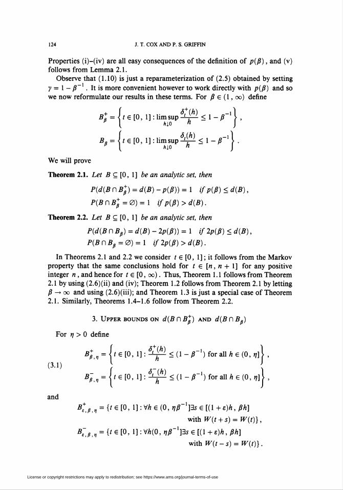
we now reformulate our results in these terms. For ß e (1, oo) define

Bt = \te[0, l]:limsup-í-P < 1 -ß~x \ ,[ hio n )

BH = \te[0, l]:limsup-4^< l-ß~l\ ■{ hlO tl J

We will prove

Theorem 2.1. Let B C[0, 1] be an analytic set, then

P(d(BxxB+ß) = d(B)-p(ß)) = 1 ifp(ß) < d(B),

P(BxlB+ß=0) = l ifp(ß)>d(B).

Theorem 2.2. Let B ç[0, 1] be an analytic set, then

P(d(B n Bß) = d(B) - 2p(ß)) = 1 if 2p(ß) < d(B),

P(B xxBß=0) = l if 2p(ß) > d(B).

In Theorems 2.1 and 2.2 we consider t e [0, 1] ; it follows from the Markov

property that the same conclusions hold for r e [«, « + 1 ] for any positive

integer « , and hence for t e [0, oo). Thus, Theorem 1.1 follows from Theorem

2.1 by using (2.6)(ii) and (iv); Theorem 1.2 follows from Theorem 2.1 by letting

ß —y oo and using (2.6)(iii); and Theorem 1.3 is just a special case of Theorem

2.1. Similarly, Theorems 1.4-1.6 follow from Theorem 2.2.

3. Upper bounds on d(B xx Bß) and d(B n Bß)

For t] > 0 define

(3.1)

and

B¡ tti = 11 e [0, 1] : ̂ < (1 - ß x) for all h e (0, t]]]

B~ n = It e [0, 1] : ^ < (1 - ß~x) for all h e (0, «]

</,,, = it e [°> 1] : VA € (0, t]ß l]3s e [(1 +e)h, ßh]

with W(t + s) = W(t)},

K,ß,„ = {*£ [°> !]: v^(0, nß-X]3s e [(l+e)h,ßh]

with W(t-s) = W(t)}.



In order that the definition of Bc „ „ make sense we adopt the convention that

W(u) = -oo for u < 0. For t]x < t]2

(3-2) Bl^Bli2>while for ßx < ß2

(3.3) limB+ñ „CB+ñ ClimB+ñ „.X ' w|0 Pi ' 1 - P\ - r|0 P-i • 1

The following observation is central to our methods for obtaining bounds on

the size of Bt and hence on Bß : if ßx < ß2, and e > 0 is small enough

that 1 - (1 + e)ß2x > 1 - ßxx, then

(3-4) Bt^BU,r

To prove this, suppose t £ B* ß , and hence that for some h e (0, t]ß2 ] we

have W't + s) ¿ W(t) for all s'e [(1 + e)h, ß2h]. Then either

A = {(t + s, x) : ( 1 + e)h < s < ß2h and W't) -(ß2-(l+ e))h <x< W(t)}

or

A = {(t + s, x) : (1 + e)h < s < ß2h and W(t) <x< W(t) + (ß2-(l+ e))h}

satisfies

AÇA>2«)\G

by continuity of the sample paths (G is the graph of W(s)). Consequently,

h' = ß2h e (0, t]] satisfies

Kih') _ Kißih) . /?2-(l+e) ^ , R-rh' - ß2h -- ß2 _>1 ^ ■

So t<jLB^n, and (3.4) follows.

Similarly, the analogous versions of (3.2)-(3.4) for Bß , Bß , and B~ ß

are valid. We now give an estimate on the size of 5+ „ „. Let

9-'t) = o{W's) :0<s<t}.

Proposition 3.1. Fix ß > I, e e (0, ß - 1) and p > 0, and assume that

E[Zp(e, ß)\ < 1. Then for any n > 0 there exists C < oo such that for all

v > 0 and all Ç sufficiently small,

(3.5) P([v,v + QxxB+£ß^O\F(v + Q)<Ci;p a.s.

Proof. By the Markov property, it suffices to consider the case v = 0. Choose

q > p and ßx > ß such that E[Zq(e, ßx)] < 1 . Fix a g (0, 1) such that

A-Q > P . and assume that

,<(Lzl)""-\lß-l ) 2



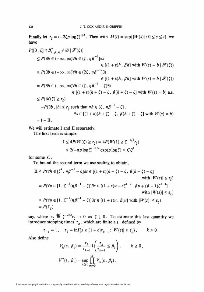
Finally let rr = (-2ÇplogQx/2. Then with M(t) = sup{\W(s)\ : 0 < s < t} we

have

< P(3b G (-00, oo)VA G (C, rjß X]3s

< P(3b G (-oo, oo)VA G (2£, t]ß X]3s

= P(3b G (-oo, oo)VA e(C,T]ß X - C]35

P([0,C]xxBlßll #0|^(O)

G [( 1 + e)A, jff A] with W(s) = b \ &{£))

e [( 1 + e)h, A A] with W(s) = b \ 9~(Q)

-Q3s

e[(l+ e)(h + 0 - C, ß(h + C) - C] with W(j) = A) a.s.

< P(Af(C) > rr)

+P(3b, |A| < rr such that VA G (C, ̂ 7^_1 - C],

35 G [(1 + e)(h + C) - C, 0(A + C) - f] with W(s) = b)= I + II.

We will estimate I and II separately.

The first term is simple:

I < 4P(W(C) > rr) = 4P(W(1) > C1/2rr)

< 2(-nplogQ'x/2exp(plogQ < CC.P

for some C.

To bound the second term we use scaling to obtain,

II < P(VA G [C", riß-1 - dis G [( 1 + e)(A + Q - Ç, ß(h + Ç) - C]

with \W(s)\ < r,)V

= P(Vmg[1,C \riß X-Q]3se[il+e)u + et;x \ßu + (ß-l)C x]

with \W(s)\ <ec)

< P(Vw G [1, C\r]ß~x - Q]3s G [(1 + e)u, ßxu] with \W(s)\ < e{)

= P(TC)

say, where e^ = Ç~x/2rr —y 0 as C I 0. To estimate this last quantity we

introduce stopping times xk , which are finite a.s., defined by

t_j = 1, rk-M{s>(l+e)tk_l:\W(s)\<e¡.}, k>0.

Also define

- xk , Jk_Vki£yßx) = t-J^1 x -^ ' ^°'

A:

V*(e,ßx) = suo\\Vm(E,ßx).k^m=0



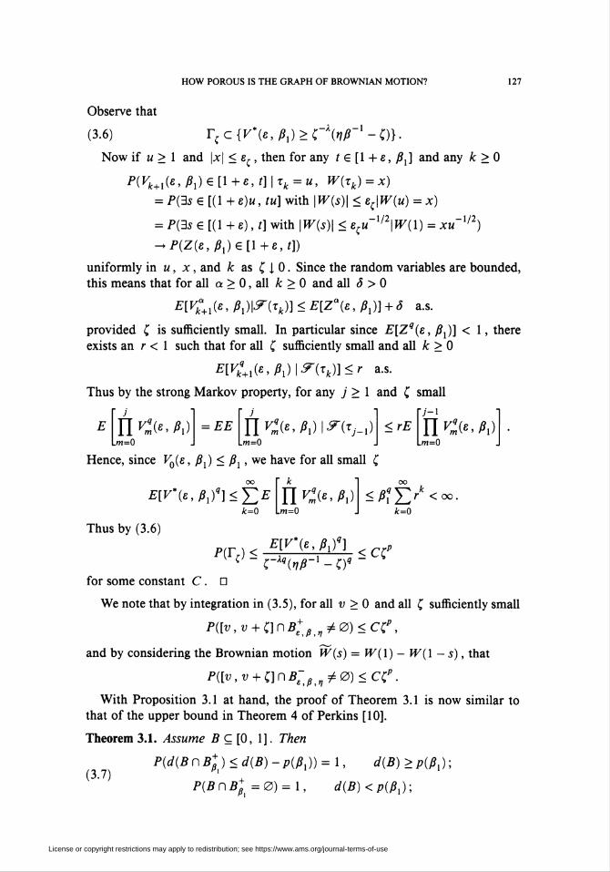
Observe that

(3.6) r(c{V*(e,ßx)>C\vß~y-0}-

Now if u > 1 and |jc| < ef, then for any t e [1 + e, ßx] and any k > 0

P(Vk+l(e, ßx)e[l+e,t]\rk = u, W(xk) = x)

= P(3s G [(1 + e)u, tu] with \W(s)\ < er\W(u) = x)

= P(3s e[(l+e),t] with \W(s)\ < eru~x/2\W(l) = xu~x'2)

^P(Z(e,ßx)e[l+e,t])

uniformly in u, x , and k as C I 0. Since the random variables are bounded,

this means that for all a > 0, all k > 0 and all ô > 0

E[Vka+x(e,ßxW(Tk))<E[Za(e,ßx)] + S a.s.

provided Ç is sufficiently small. In particular since E[Zq(e, ßx)\ < 1, there

exists an r < 1 such that for all C sufficiently small and all k > 0

E[Vk\x(e,ßx)\F(Tk)]<r a.s.

Thus by the strong Markov property, for any j > 1 and £ small

IlKi^ßxLm=0

= EE UV^yßx)\^j-x)Lw=0

<rE n^v^i)m=0

Hence, since VJe, ßx) < ßx, we have for all small Ç

E[V*(e,ßx)q]<Y,Ek=0

Thus by (3.6)

UK(eyßx)m=0

</??jy<oc.

k=0

E[V*(e ßxn < ,c rX9(r,ß-x-o9~

for some constant C. D

We note that by integration in (3.5), for all v > 0 and all C sufficiently small

P([v,v + C]xxBlßri^0)<CCP,

and by considering the Brownian motion W(s) = W(l) — W(l—s), that

P([v,v + QxxB-ß ni0)<C?.

With Proposition 3.1 at hand, the proof of Theorem 3.1 is now similar to

that of the upper bound in Theorem 4 of Perkins [10].

Theorem 3.1. Assume B ç [0, 1]. Then

P(d(BxxB+)<d(B)-p(ßx)) = l, d(B)>p(ßx);(3.7) * +

PiBxxB+ß =0) = 1, d(B)<p(ßx);



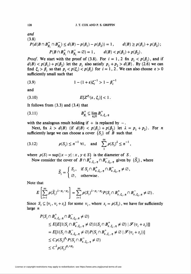
and

(3.8)P(d(BxxB+ßiXxBß2)<d(B)-p(ßx)-p(ß2)) = 1, d(B)>p(ßx)+p(ß2);

P(BxxB^xxB~2 = 0) = 1, d(B)<p(ßx) +p(ß2).

Proof. We start with the proof of (3.8). For i = 1,2 fix pi < p(ßA, and if

d(B) < p(ßx) +p(ß2) let the p¡ also satisfy px+p2> d(B). By (2.6) we can

find t,i > ßi so that pi < p(C¡) </>(/?,) for i = 1,2. We can also choose e > 0

sufficiently small such that

(3.9)

and

(3.10)

l-(l+e)^x>l-ß;x

E[ZPi(e,L)]<l

It follows from (3.3) and (3.4) that

(3.11) B+R ClimÄ+« „

with the analogous result holding if + is replaced by - .

Next, fix a > d(B) (if d(B) < p(ßx) + p(ß2) let X = px+p2). For n

sufficiently large we can choose a cover {S¡} of B such that

(3.12) p(St)<n 'W, and f^p(Sif<n X,

where p(S) = sup{|.x - y\ : x, y e S} is the diameter of S1.

Now consider the cover of 5fl5t+, „ n B~ * „ given by {SA , where

~ (S„ if5¡n<íi,í/n5-Í2^0,

1 0, otherwise.

Note that

X>WÇ A-Pi -Pi

i=x¿ZPVtPx~**Vi"<^K^.n*®)'i=X

Since S¡ ç [vi, vi + s¡] for some vi, where s¡ = p(S¡), we have for sufficiently

large «

P(S^BU,nnBe,i2,^0)

<E[E[l(SixxB;(2^0)l(S¡xlBltít¡¿0)\F(vi + si)]}

= E[l(S¡xxB;:Í2^0)P(SinBli¡n¿0\F(v¡ + si))]

<Cp(Si)p>P(SixxB:An¿0)

< C2p(Si)Pi+Pl



by Proposition 3.1 and the remarks following it. Hence by (3.12) and Fatou

00

(3.13) liminfYp(Sif~Pl~Pl = 0 a.s.R—»OO

1=1

We now consider the cases d(B) > p(ßx) + p(ß2) and d(B) < p(ßx) + p(ß2)

separately. In the former case, since X > d(B) was arbitrary, (3.13) implies

that for any t] > 0

nd(BxxB+eArixxB-^)<d(B)-px - p2) = 1.

By letting n [ 0 and noting (3.11), this gives

P(d(B xx £+ xx B~2) < d(B) -Px-p2) = l.

Since pi < p(ßj) are arbitrary, this proves the first part of (3.8). If d(B) <

Piß\) +piß2), then since we chose X = px+p2, (3.13) implies for all r¡ > 0

^n<íi;„n5-Í2>^0) = O.

Letting t] I 0 completes the proof of (3.8).

The proof of (3.7) is similar, but easier. Fix px < p(ßx), and if d(B) < p(ßx)

let px also satisfy px > d(B). Choose £x > ßx so that px < p(Çx) < p(ßx),

and choose e > 0 sufficiently small such that

(3.9)' l-fl+^-Sl-^1

and

(3.10)' E[ZPi(e,^x)]<l.

Next, fix a > d(B) (if d(B) < p(ßx) let X = px). For « sufficiently large we

can choose a cover {S¡} of B satisfying (3.12). Define {S¡} by

S. = IS<> [{SinBU,^0>' [0) otherwise.

By the remarks following Proposition 3.1 we have

P(SixxB+tn*0)<Cp(Si)*

Thus

EpW*PKo/-i=X

0,

and so by Fatou

OO

(3.13)' UminfY p(SAX~p> =0 a.s.1=1

The remainder of the argument is as before. D

Remark. The estimate (3.5) can be used to give a proof (though not necessarily

the most elementary one) of (1.6). Fix t > 0, and note that for any ß > 1 and



e e (0, ß - 1) we can find p > 0 such that E[Zp(e, ß)] < 1. By Proposition

3.1, for any t] > 0 there exists a finite constant C such that for all sufficiently

small C

p([t,t + t;]xiBlß^0)<ct;p.

This implies

P(teB+tJ3n) = 0,

and consequently we have

This means that a.s. for every t] > 0 there exists A G (0, r¡] with S*(h) >

h(l-(l+e)ß~x). Thus

p[limsup^l> i _(!+£)£-> ] = i.V mo « y

Letting ß î oo completes the proof of (1.6).

4. Lower Bounds on d(B n 5Í ) and d(B xx Bß)

For ß > 1, e G (0, yS - 1) and X > 0, define

(4.1) T0(e) = inf{j>l:H/(s) = H/(0)}, A0(e, /?, X) = T0(e)l(r0(e) < 0),

(t0 and A0 do not actually depend on e and X, but it simplifies the notation

below to include these parameters in their definitions) and for k > 1

(4.2)rk(e) = inf{s > (l+e)rk_x(e) : W(s) = W(0)},

Ck(e,X) = {3u,v e [rk_x(e), (1 +e)rk_x(e)]

with W(u) = W(0)+Xxxkl2x(e) and W(v) = W(0) - XTXk/2x(e)},

k

Xk(e, ß, X) = X0(e, ß, X)llYJe, ß, X),m=X

X*(e,ß,X) = supXk(e,ß,X).k>0

First observe that ^(e) < oo a.s. for all k. Next, by the scaling and strong

Markov properties, Yk(e, ß, X), k > 1 are i.i.d. with common distribution

P(Yx(e,ß,X)e[l+e,t])

= P(3u,ve[l, l+e] with W(u) = 1^(1) +a and IT(W) = w(l)-X,

and 35 g [(l+e), t] with W's) = W(l))



for 1 + e < t < ß, with all remaining mass at the origin. In particular, if =>

denotes weak convergence, then

Yx(e, ß,X)^Z(s,ß) as a 10.

Thus for all a > 0

(4.3) E[Yxa(e,ß,X)]-+E[Za(e,ß)}.

Also by the scaling and strong Markov properties A0(e, ß, X) is independent

of {Yk(e, ß, a) ; k > 1} , and hence Xk(e, ß, X) is a product of independent

random variables.

In what follows we will often consider two independent Brownian motions

Wx and W2 defined on the same probability space Q. We denote the corre-

sponding random variables in (4.2) by Yk(i; e, ß, X), Xk(i; e, ß, X), etc. for

i = 1,2. We will use the notation an « bn to mean ajbn is bounded above

and below by finite, nonzero constants which are independent of « .

Lemma 4.1. Fix S > 0, ßx > 1, ß2> 1, and assume that p(ßx) + p(ß2) < S .

Then for all e > 0 sufficiently small there exists a X > 0 and a p e (0, S) such

that for all b >S,

E[(X* (l;e,ßx,X)AX*(2;e,ß2,X)A n)b] « n~p,

where a Kb = min(a, b).

Proof. Let qx > p(ßx) and q2 > p(ß2) satisfy qx+q2<ô . Then by (2.6) and

(4.3) for all e > 0 sufficiently small we can find X > 0 so that E[Yx'(i ; e, ßi, X)\

> 1 for i = 1,2. So by reducing qx and q2 we can find px > 0 and p2> 0

satisfying px +p2 <S and

E[Yp-(i;e,ßi,X)]=l.

Thus, recalling that Xk(i ; e, ßx., X) is a product of independent random vari-

ables, it follows that Xp'(i ; e, ßx.., X) is a nonnegative martingale. Hence

Xp'(i; e, ßj, X) converges a.s., necessarily to zero, as k —> oo. Next, for r > 1

set

Tr(i) = inf{k:Xp'(i;e,ßi,X)>r}.

Since

Xp^i)Ak(i;e,ßi,X)<ßir,

dominated convergence implies

E[XpA(i; e, ßt, X)] = E[Xp'(i)Ak(i;e,ß., X)]

->E[Xp-{l)(i;e;ßi,X);Tr(i)<oc)

as k -> oo . Observe that on {Tr(i) < oo} = {X*(i;e,ßit X)p¡ > r} we have

r<XpT'{i)(i;e,ßi,X)<ßir.



Thus

/^■(/Vr1 < P{X*(i\e, ßt,kf* >r)< p¡r-x

where

p[=E[XpA(i;e,ßi,X)]>0.

Now let p = px+p2, and assume that b > ô . Then since p < S

E[(X*(l;e,ßx,X)AX*(2;e,ß2,X)r\n)b]

= i" brb~XP(X*(l ;e,ßx,X)> r)P(X*(2;e, ß,,X)> r)drJo

nnb~p. D

We will need to consider slightly smaller sets than Bß and Bß defined as

follows: for a > 1 let

"A* (A) = {(s,x):t<s<t + h, f(t) - ah < x < f(t) + ah},

aS+(h) = sup{|A|1/2 : A ç ÛA+(A), A n G = 0},

aB\ = \te\0, l]:limsup-^-^ < 1-^_11 ,p { hio h J

with analogous definitions if + is replaced by - . Observe that since a > 1,

aô*(h) > S+(h) and aS;(h) > 6~'h), hence

(4.4) aBß ç Bß and aBß ç Bß .

For i = 1,2, let aA¡(i;h), aôt+(i;h), aBß(i) and Bß(i) be the quanti-

ties analogous to flA*(A), aôf(h), aBß and Bß defined relative to IT., and

similarly with + replaced by - . Define

9¡(t) = o{Wi(s) :0<s<t}, S?(t) = o{?['t) u F2(t)} .

Given a subset T of [0, 1] x Q., let T(œ) = {t e [0, 1] : (t, œ) e T}. In

what follows we will often write T for T(w) when the meaning is clear. The

following proposition is based on Proposition 14 in [10].

Proposition 4.1. Let T be a &(t) progressively measurable subset of [0, 1] x Q

such that T ¿s closed a.s. Then for any a > 1, and Çx, t\2 > 1

p({d(r)>P(c:x)+p(z2)}\{muBi(i)xxuB;2(2)¿0}) = o.

Proof. Since the proof of this result is rather lengthy, we divide it into six

steps. In the first two steps certain parameters are fixed and various sequences

of random variables are defined. Steps 3 and 4 are concerned with some purely

geometric arguments used to describe certain events in terms of these random

variables. In Step 5 the problem is reduced to equation (4.15), which is then

verified in Step 6.



Step 1. We may assume p(£x) + p(£2) < 1, else the result is trivial. Fix S e

(p(Cx)+p(c;2), 1) and let ß, e (1, {,) for i = 1, 2 satisfy

(4.5) p(ßx)+p(ß2)<o.

Choose e > 0, X > 0 and p e (0, S), so that the conclusion of Lemma 4.1

holds, and for ¿=1,2

(4.6) (1+«)£<«,.

Let ß = ßx V ß2 and ß' = ßx A ß2, and choose M so that

(4.7) M>/(1+£)2ß'(l + e)-l

Finally, let

(4.8) A<ßX2M~2.

The parameters S , /?, , ß2, p , e , X, M and A have now been fixed.

Step 2. For « > 1 (an integer) and ï = 1,2 define

t0(i) = inf{* > «-1 : H/.(5) = H/(0)}, A0(/) = T0(/)l(t0(/) < ßf),

and for k > 1

tfc(i) = inf{s > (l+e)rk_x(i) : W,(s) = ^(0)},

Ck(i) = {3u,ve[rk_x(i),(l+e)rk_x(i)]

with W¡(u) = Wt(0) + XxXkl2x(i) and W,(v) = W^O) -XxXk'2x(i)},

it

[yM(i), a*(/) =

m-1

Then by scaling

(4.9) «A*(/) = A*(/;e,^.,A), nX* = X*(l; e, ßx, X) AX*(2; e, ß2, X)

Step 3. For any n < A

(4.10) {ßX* >t]}ç {VA G [y?«"1, ß~2n]3u(i), u(í) G [A , A(l + e)/?,.]

with IT(w(/)) = H^(0) + Mh and

IT.(?j(/)) = H/(0)-A/A, 1 = 1,2}.

To see this, suppose ßX* > r\, and h e [ßn~x, ß~2tj]. Then for i = 1,2

we can find a k = k(i) such that Xk(i) > ßh . But this means that for some

m < k,

(4.11) h<x(i)<ßh

Xkii)=Xoi¿)UYmii)y X*(i) = supXk(i), A*=A*(1)AA*(2).

* / *\ d t/* / . fX T -, T/"* ¿/ V* /



and Cm+X(i) occurs. In particular there exist

u(i),v(i) e [tji), Tw(i)(l + 8)] c [h,h(l+e)ß]

such that

Wi(u(i)) = W(0) + Xxm(ï)X'2,

rVi(v(i)) = W(0)-Xrm(i)X/2.

But by (4.8) and (4.11), since A < ß~2t] < ß~2A

temii)l/2 > Mx/2 > MiAß~x)x/2hx/2 > Mhßx/2 > Mh

since ß > 1. Thus (4.10) holds. The reason for using ßX* rather than X*

on the left-side of (4.10) is that clearly {A* < u} e &ißu), and so ßX* is a

stopping time.

Step 4. Let

Z)„ „ = {i g T : VA g [ßn~x, ß-2t]]3u(i), v(i) e [A, A(l +e)ßi],

with W¡'t + u(i)) = W¡(t) + Mh

and W.'t + v(i)) = W¡(t) -Mh, i = 1, 2},

and let 6( be the usual shift operator. Then for every co

(4.12) {teT:ßX*oQt>t]}CDnt},

oo

(4.13) \JC\DnncTxxaB¡(l)xAaB¡2(2).r>0r=1

Assertion (4.12) follows immediately from (4.10). To see (4.13), fix n > 0 and

suppose that t e xc]7=xDn^- Let A G (0, ß~2r]], and assume that for either

i = I or 2ACaA+(i;h)

where

A=(t, Wi(t)) + ([sx,s2]x[xx,x2])

and

S2-Sx=X2-Xx=h(l-((l+E)ßi)-X).

We will show that the graph of Wi intersects A, and hence

A - (l+e)ßl~ £,.

which implies teYxxaB^(l)n aB+ (2). To do this, observe that

and

_1_(l+a)^-*»-



This last fact follows from

-'. = ( » - tt-tV) ( TT^(l + e)/?,. » V (l+e)ßiJ\(l+e)ßi

Now let tí = ((1 + e)ßA~xs2 and note that sx < tí < s2 < A. Since t G

CC=X Dn n tnere mUSt eX^St M(') ' U(/-) £ t^' > ̂ 't1 + e)/*/J - l5l ' S2J Witn

WAt + u(i)) = WAfy + Mh', WAjt + v(i)) = W¡(t) - Mh'.

By the definition of M and the previous inequalities we see that Mh' > ah,

and thus path continuity implies the graph of Wf. must intersect A. This

establishes (4.13).

Step 5. Let

{k k

J2 PiSf : T ç (J St, 5, are closed intervals¡=i i=i

with p(S¡) < t], k > 1 \ ,

and

£• = {/J -» oo as n J, 0}.

Thus

(4.14) £ D {d(T) > 0}.

Finally let

In the next step we will show that

(4.15) pIe\\JC\G,,A=0.V R>0 R J

Now clearly lj„>0 D„ Gn , D {U„>0 H« ö„,„ ^ 0} . and since a.s. Dn>n is com-

pact and Dn+Xt}CDnrt

^iun^„\(un^R,^4)=0-\^>0 r y r>0 R J y

Thus by (4.13), (4.14) and (4.15)

P({d(T)>o}\{TnaB¡(l)xxaB¡2(2)í0}) = O.

Letting S i p(¿¡x) + p(¿¡2) then completes the proof of the proposition. Thus it

remains to prove (4.15).

Step 6. Define

C, =inf{/>0:iGT}A2, ax = C, + (ißX* ° Gf ) A 1),



and for k > 2

Ck = inf{t >ok_x:teY}A2, ok = Ck + HßX* o er¡) A 1)

where inf(0) = oo. Then Çk and ok are stopping times since T is progres-

sively measurable and ßX* is a stopping time. Observe also that if Çk < 1,

then Cfc € T a.s. since T is closed a.s. Let

Nx=sup{k:i;k<l},

where sup(0) = 0. Then

N

rçlj^>^ a-s-k=X

Thus by (4.12)

P(E"Gln)<p(E, maxNiok-t;k)<t]}

<P\E,£(<Jk-Çk)S>HtV k=x

/*,

<P(E,Hri<x) + P\¿2i°k-tk)Ó> x

.k=X

d ov*

for any x > 0.

We now estimate the last term above. Since (rjj. - Çk) = "ßX* A 1, and C,k

is independent of ak- Çk , we have for any b > 0

k=X

= E £kc,<dk-c*)äk=X

= ¿ZPUk < l)E[(ok - W I = E[Nx]E[(ßX* A 1)*].k=X

With b = ô this implies

if.

fc=i

^[AI]A[(ySA*Al)<5].

.A,With 6=1 and the fact that 2 > £¿.i,(crfc - ÍJ we get

2£[#,]<

ThusA',

it=i

- E[ßX* A 1]

2£[(ySA*Al)<?]<

E[ßX* A 1]



Now by (4.5), (4.9), and Lemma 4.1, there exists p e (0,0) such that for

b>ô,

E[(ßX* A l)b] = n~bE[(X*{l; e,ßx,X)A A*(2 ; e, ß2, X) A n)b] « n~p .

This implies that there exists a finite constant c independent of « such that

e Bff*-w *'•_fc=i

and thus by Chebyshev

P(ExxGcnn)<P(E,Hn<x) + clx.

For any r > 0 we can choose x sufficiently large and t]0 sufficiently small

so that

for all « . Now let G = f]n Gn . Since Gn+X ç Gn we have

P(ExxGc%)<r.

Equation (4.15) now follows from the fact that G T as t] [ . D

Remark. Let C ç [0, 1] be closed. By taking T = C x Q in Proposition 4.1

we have for every a > 1

(4.16) P(CxxaB^(l)x\aB¡2(2)¿0)=l

provided p(^x) + p(Ç2) < d(C). This will be used in the next result.

Theorem 4.1. For every analytic set B ç [0, 1] and every a > 1

P(d(BxxaB+ß)>d(B)-p(ß)) = l,

P(d(BDaBß)>d(B)-p(ß)) = l.

Proof. It suffices to prove the aBß case since we obtain the aBZ case by con-

sidering W(t) = W(l) - W(l - t). We may assume that p(ß) < d(B), else

there is nothing to prove. Since B is analytic, for any e > 0 there exists a

compact set C ç B such that d(C) > d(B) - e . Assume that e is sufficiently

small that d(C) > p(ß). Then for any ßx satisfying p(ßx) < d(C) - p(ß) we

have by the remark above

z>(Cna5;i(l)nal?;(2)^0) = i.

Thus

(4.18) P(CnaB¡í(l)xlaB~¡¡(2)¿0\ W2) = 1 a.s.

Since for a given W2, the random set CnaBß(2) may be considered fixed under

P(- | W2), and aB+ß(l) ç B+ß(l), we can apply (3.7) with B = C xx aB¡(2) to

obtain

P(d(CxxaB+ß(2))>p(ßx)\W2) = l a.s.



ThusP(d(CilaB+ß(2))>p(ßx)) = l

and hence

P(d(BxxaB+ß(2))>p(ßx)) = l.

Since p is continuous, ßx is arbitrary subject to the requirement that p(ßx) <

d(C) - p(ß), and e > 0 is arbitrary, we are done. D

Setting a = 1 in (4.17) together with (3.7) then gives Theorem 2.1. Next we

turn to Theorem 2.2.

Theorem 4.2. For every analytic set B ç [0, 1] and every a > 1

P(d(BDaB+ßiXxaB-ß2) > d(B)-p(ßx)-p(ß2)) = 1.

Proof. We may assume p(ßl)+p(ß2) < d(B). Fix e > 0 sufficiently small that

Pißi)+Piß2) < diB) - e. Choose C ç B compact such that rf(C) > d(B) -e,

and let /?3 satisfy

(4.19) p(ßx)+p(ß2)+p(ß3)<d(C).

Arguing as in Theorem 4.1, it suffices to show

(4.20) P(Cx\aB+ß^(l)xxaB~2(l)x\aB+ßp)^0\Wx) = l a.s.

(let ß = Cn^(l)n aB~ß(\) in (3.7), etc.). To prove this we will show that

if t] is sufficiently small, then

(4.21) P(CxAaB+ßi(l)xxaBß2>ri(l)naB+ß}(2)^0) = l

where

aB~2 „(1) = it G [0, 1] : S< (lh ; k) < (1 - ß2X) for all A G (0, «] j .

Since aB~ (1) eaB~(l), (4.20) then follows.

In order to prove (4.21) all we need to do is show that

(4.22) P(d(CxxaB-ß2^(l))>p(ßx)+p(ß,)) = l

and apply Proposition 4.1 (T defined by T((o) = CxxaBß (I) is a.s. closed

and progressively measurable). To do this choose ß < ß2 such that p(ßx) +

p(ß)+p(ß3)<d(C). By Theorem 4.1, since d(C) -p(ß) > p(ßx) + p(ß3),

P(d(CxxaBß(l))>p(ßx)+p(ß3)) = l.

But lim^o aB~ ( 1 ) D aB~ ( 1 ), and hence

limJ(Cn^,(l))>d(Cn^(l))>/)(/l1)+^3) a.s.

Thus (4.22) holds. G

Combining the results in Theorem 3.1 and Theorem 4.2 with (4.4) we see

that for every analytic set B ç [0, 1] and every a > I, B C\ aBß n aB~ = 0

a.s. if 2p(ß) > d(B), while if 2p(ß) < d(B) then

(4.23) P(d(B xx aB+ß xx aBß) = d(B) - 2p(ß)) = 1.



Thus to complete the proof of Theorem 2.2 it suffices to prove

Proposition 4.2. If a > 2ß(ß - l)~x then for every co

aB+ßnaBßCBßCB+ßxlBß.

Proof. Clearly Bß ç Bt xx Bß . To prove the other inclusion we argue by

contradiction. Thus assume that t G (aBß n aBß)\Bß. Since a > 1, te

(BßxxBß)\Bß . Hence there exists a sequence hn [ 0 and a sequence of squares

An such that

A„ÇA,(A„)\G,

A„nAX)/0, A„nAi-(A„)^0,

\An\lllh~nl>v>i-ß-x.

By taking a further subsequence if necessary we may assume that at least half

of An intersects A^(hn), i.e.

(4.24) \AnnA¿(hn)\1/2h;l>v/V2,

(if not, argue using A~(AJ in place of A*(An) in what follows). But then by

the definition of a,

which contradicts t eaBß . o

Acknowledgment. We would like to thank Dan Waterman for bringing this prob-

lem to our attention.

References

1. M. T. Barlow and E. A. Perkins, Brownian motion at a slow point, Trans. Amer. Math. Soc.296(1986), 741-775.

2. B. Davis, On Brownian slow points, Z. Wahrsch. Verw. Gebeite 64 (1983), 359-367.

3. B. Davis and E. A. Perkins, Brownian slow points: the critical case, Ann. Probab. 13 (1985),779-803.

4. A. Denjoy, Leçons sur le calcul des coefficients d'une serie trigonometrique. Part II, Métrique

et topologie d'ensembles parfait et de fonctions, Gauthier-Villars, Paris, 1941.

5. E. P. Dolzhenko, Boundary properties of arbitrary functions, Math. USSR 12 (1967), no. 1,1-12.

6. J. Foran, Continuous functions need not have a-porous graphs. Real Anal. Exchange 11

(1985-86), 194-203.

7. C. Goffman, The graph of Brownian motion is not strongly porous, Preprint, 1988.

8. P. A. Greenwood and E. A. Perkins, A conditioned limit theorem for random walk and

Brownian local time on square root boundaries, Ann. Probab. 11 (1983), 227-261.

9. _, Limit theorems for excursions from a moving boundary, Theor. Probab. Appl. 29

(1984), 517-528.



10. E. Perkins, On the Hausdorff dimension of the Brownian slow points, Z. Wahrsch. Verw.

Gebiete 64 (1983), 369-399.

11. B. S. Thomson, Real functions, Springer-Verlag, New York, 1985.

12. L. Zajicek, Sets of o-porosity and sets of a-porosity (q), Casopis Pëst. Mat. 101 (1976),

350-359.

Department of Mathematics, Syracuse University, Syracuse, New York 13244-1150

E-mail address (J. T. Cox): [email protected]


how porous is the graph of brownian motion? · 2018-11-16 · abstract. we prove that the graph of...

Documents