-how new technologies impact a conventional intersection

Technologies and Urban Traffic

-How New Technologies Impact a Conventional Intersection

Lingyu (Simon) Li

Thesis Paper

Advisor: Professor Anthony Vanky

Reader: Professor Lucius Riccio

Columbia University

Graduate School of Architecture, Planning, and Preservation

Monday, May 4, 2020

II

Preface This research originated from my passion for future road transportation. The

technology evolvements during the recent decades empowered us with the ability to

push urban traffic to a new level where it is cleaner, more efficient, and safer. My

research is only a small step forward, yet I hope it a starting point of my career, a career

to make every journey more enjoyable.

In truth, I could not have achieved my current level of success without a strong

support group. First of all, my parents, Mr. �� and Mrs. ��, who supported me

with love and understanding. And secondly, my thesis group members, my advisor Dr.

Anthony Vanky, and my reader Dr. Lucius Riccio, each of whom has provided patient

advice and guidance throughout the research process. Last but not least, my friends,

who helped me stay positive during this hard time. Thank you all for your unwavering

support.

2020 is hard for us all, stay positive, we can win this war.

III

Abstract Urban population swelling and the expansion of people’s need for transportation

make traffic congestions an important urban deficiency faced by cities over the globe.

Fortunately, emerging information technologies grant us many possible ways to improve

the situation. This research built intersection traffic models in PTV Vissim platform to

test the performance of Fluctuated Traffic Light technology, Vehicle to Infrastructure

(V2I) technology, and Vehicle to Vehicle (V2V) technology under both peak and bottom

volumes. The results indicate that these emerging technologies have the potential to

boost traffic performance. V2I method functions the best under higher traffic volumes,

while V2V tested to be the best under lower traffic volumes. Take a step back, from

urban planning perspective, these technologies are still in their early stages and seems

far from reality, however, planners should be prepared for the challenges it may pose.

IV

Table of Contents

PREFACE............................................................................................................................................................II

ABSTRACT.......................................................................................................................................................III

CHAPTER1:INTRODUCTION.......................................................................................................................1

CHAPTER2:RESEARCHDESIGN..................................................................................................................4

2.1RESEARCHQUESTION....................................................................................................................................42.2RESEARCHPROCESS......................................................................................................................................4

CHAPTER3:LITERATUREREVIEW............................................................................................................6

3.1CONVENTIONALANDFLUCTUATEDTRAFFICLIGHTCONTROL.....................................................................63.2WAVEPROTOCOL......................................................................................................................................103.3PEDESTRIANSANDBIKERS..........................................................................................................................143.4GREENHOUSEGASES(GHG)EMISSIONFROMTRANSPORTATION.............................................................173.5INTERSECTIONPERFORMANCEEVALUATION..............................................................................................18

CHAPTER4:METHODOLOGY.....................................................................................................................19

4.1STUDYSITESELECTION...............................................................................................................................194.2INITIALDATARESEARCH............................................................................................................................234.3SIMULATION................................................................................................................................................264.4TRAFFICCRITERIADEVELOPMENT.............................................................................................................36

CHAPTER5:RESULTS..................................................................................................................................39

5.1DELAYSFORINTELLIGENTTRAFFICLIGHTS...............................................................................................395.2DELAYSFORV2I..........................................................................................................................................425.3DELAYSFORV2V........................................................................................................................................445.4DELAYCOMPARE.........................................................................................................................................455.5THROUGHPUT..............................................................................................................................................465.6GHGEMISSION............................................................................................................................................46

V

CHAPTER6:DISCUSSION............................................................................................................................48

6.1RESEARCHLIMITATIONS.............................................................................................................................486.2RESULTSDISCUSSION..................................................................................................................................496.3CHALLENGESANDOPPORTUNITIESTOURBANPLANNERS.........................................................................51

REFERENCES...................................................................................................................................................53

APPENDIXI.RAWDATA–CURRENTSITUATION.................................................................................64

APPENDIXII.RAWDATA–ITL..................................................................................................................65

APPENDIXIII.RAWDATA–V2I................................................................................................................66

APPENDIXIV.RAWDATA–V2V................................................................................................................67

APPENDIXV.ANALYSISFULLSCRIPT......................................................................................................68

1

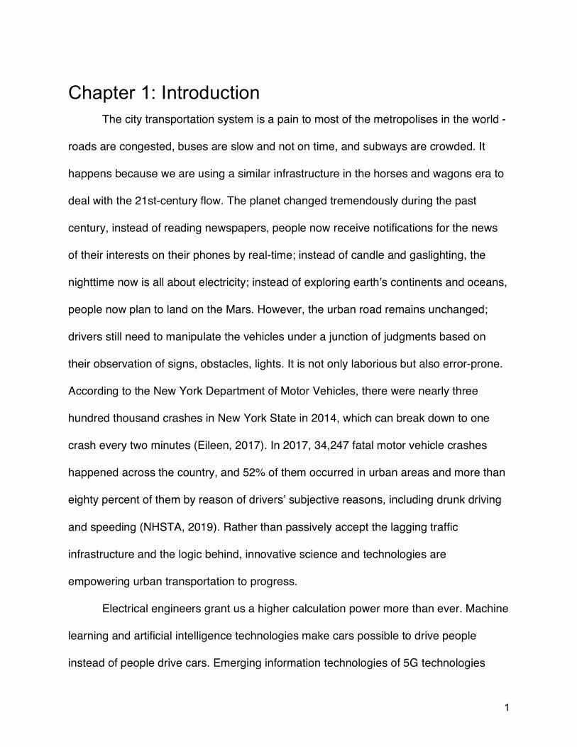
Chapter 1: Introduction The city transportation system is a pain to most of the metropolises in the world -

roads are congested, buses are slow and not on time, and subways are crowded. It

happens because we are using a similar infrastructure in the horses and wagons era to

deal with the 21st-century flow. The planet changed tremendously during the past

century, instead of reading newspapers, people now receive notifications for the news

of their interests on their phones by real-time; instead of candle and gaslighting, the

nighttime now is all about electricity; instead of exploring earth’s continents and oceans,

people now plan to land on the Mars. However, the urban road remains unchanged;

drivers still need to manipulate the vehicles under a junction of judgments based on

their observation of signs, obstacles, lights. It is not only laborious but also error-prone.

According to the New York Department of Motor Vehicles, there were nearly three

hundred thousand crashes in New York State in 2014, which can break down to one

crash every two minutes (Eileen, 2017). In 2017, 34,247 fatal motor vehicle crashes

happened across the country, and 52% of them occurred in urban areas and more than

eighty percent of them by reason of drivers’ subjective reasons, including drunk driving

and speeding (NHSTA, 2019). Rather than passively accept the lagging traffic

infrastructure and the logic behind, innovative science and technologies are

empowering urban transportation to progress.

Electrical engineers grant us a higher calculation power more than ever. Machine

learning and artificial intelligence technologies make cars possible to drive people

instead of people drive cars. Emerging information technologies of 5G technologies

2

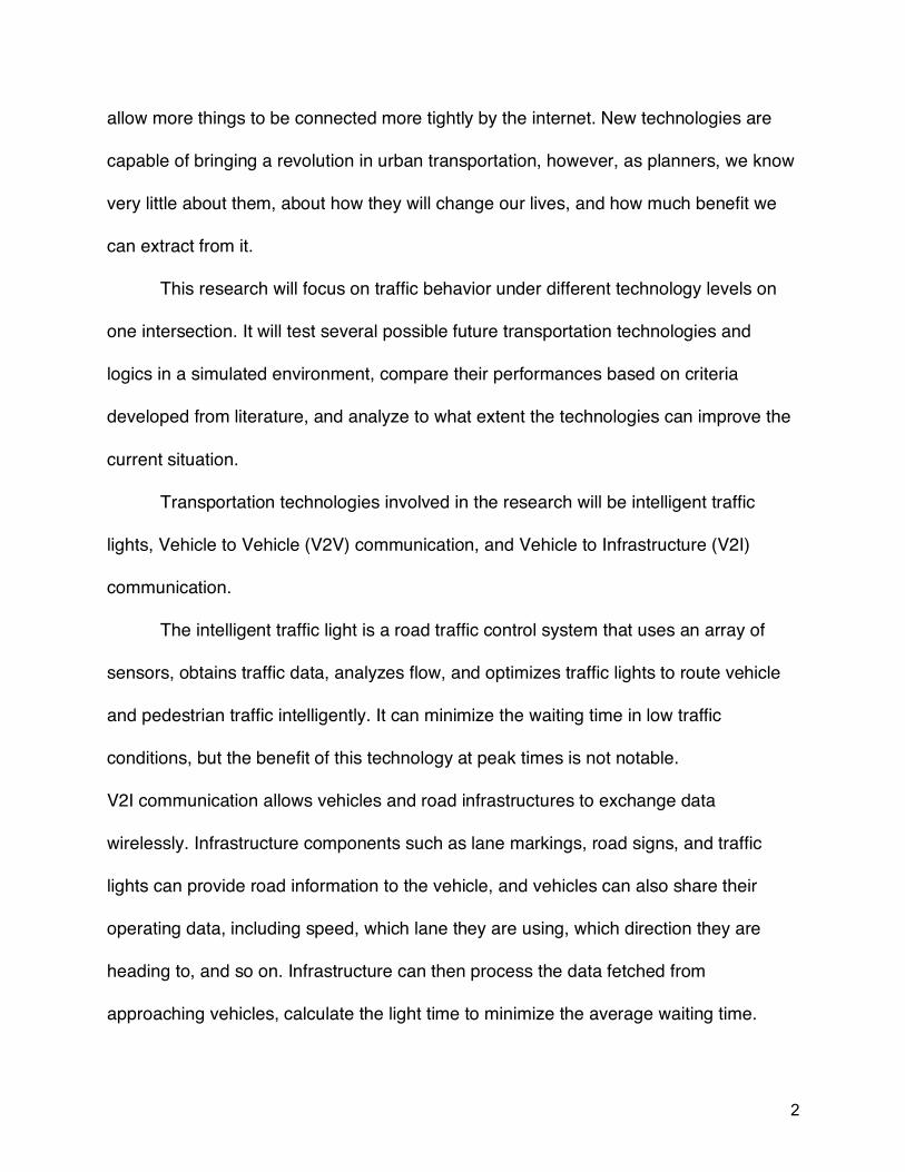
allow more things to be connected more tightly by the internet. New technologies are

capable of bringing a revolution in urban transportation, however, as planners, we know

very little about them, about how they will change our lives, and how much benefit we

can extract from it.

This research will focus on traffic behavior under different technology levels on

one intersection. It will test several possible future transportation technologies and

logics in a simulated environment, compare their performances based on criteria

developed from literature, and analyze to what extent the technologies can improve the

current situation.

Transportation technologies involved in the research will be intelligent traffic

lights, Vehicle to Vehicle (V2V) communication, and Vehicle to Infrastructure (V2I)

communication.

The intelligent traffic light is a road traffic control system that uses an array of

sensors, obtains traffic data, analyzes flow, and optimizes traffic lights to route vehicle

and pedestrian traffic intelligently. It can minimize the waiting time in low traffic

conditions, but the benefit of this technology at peak times is not notable.

V2I communication allows vehicles and road infrastructures to exchange data

wirelessly. Infrastructure components such as lane markings, road signs, and traffic

lights can provide road information to the vehicle, and vehicles can also share their

operating data, including speed, which lane they are using, which direction they are

heading to, and so on. Infrastructure can then process the data fetched from

approaching vehicles, calculate the light time to minimize the average waiting time.

3

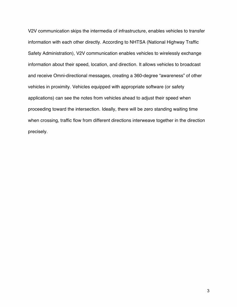
V2V communication skips the intermedia of infrastructure, enables vehicles to transfer

information with each other directly. According to NHTSA (National Highway Traffic

Safety Administration), V2V communication enables vehicles to wirelessly exchange

information about their speed, location, and direction. It allows vehicles to broadcast

and receive Omni-directional messages, creating a 360-degree “awareness” of other

vehicles in proximity. Vehicles equipped with appropriate software (or safety

applications) can see the notes from vehicles ahead to adjust their speed when

proceeding toward the intersection. Ideally, there will be zero standing waiting time

when crossing, traffic flow from different directions interweave together in the direction

precisely.

4

Chapter 2: Research Design

2.1 Research Question the research question then originated as how can commuters’ travel experience

be improved by applying new transportation technologies? Travel experience is

measured by the criteria developed from the literature of previous studies, and

transportation technologies here include fluctuated traffic light system, Vehicle to

Infrastructure communication, and Vehicle to Vehicle communication. It is important for

us as urban planners to really understand them, understand their pros and cons, utilize

them and make our cities better.

2.2 Research Process The research can be separated into three phases: information gathering,

simulation, and result analysis. Information gathering includes literature reviewing and

data fetching. Literature reviews provide ideas about simulation methods, technology

backgrounds, study site choices, and performance indicators. Data gathering involves

getting street infrastructure, traffic counts of the study site, and technology tuning

information. Simulation phase is the period where real-world situation as well as

advanced technologies are projected into simulation platforms. Result analysis means

to analyze the simulation results by fitting models using python, in order to further

illustrate the logic behind the numbers.

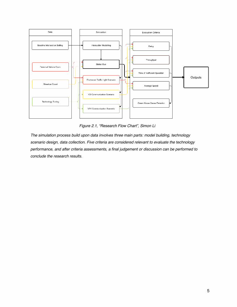
The research flowchart is shown in figure 2.1.

5

Figure 2.1, “Research Flow Chart”, Simon Li

The simulation process build upon data involves three main parts: model building, technology scenario design, data collection. Five criteria are considered relevant to evaluate the technology performance, and after criteria assessments, a final judgement or discussion can be performed to conclude the research results.

6

Chapter 3: Literature Review

3.1 Conventional and Fluctuated Traffic Light Control One of the base knowledges in understanding the how traffic flow forms and how

the intersection can help in the formation is to understand the traffic light control logics

and how it can be improved by fluctuated traffic light control algorithms.

Classical control approach and its limitations

Most of today’s traffic light control approaches are centralized and based on the

application of pre-calculated schedules with the possibility to be manipulated to adapt to

extreme traffic conditions (Porche et al., 1996). The coordination of the traffic network is

reached by applying a typical cycle time to all the nodes of multiply a basic frequency,

which is determined by the most severe bottleneck of the network (Webster, 1958). This

feature makes the conventional traffic control unilateral and often prioritizes a

unidirectional main flow (Papageorgiou, 1991).

There are several obvious disadvantages of the classical control approach:

1) The green light times are often set longer than needed to handle the inflow

fluctuation, otherwise another excessive waiting time would be triggered due to

multiple stops of the same red light (Papageorgiou et al, 2003).

2) The waiting time in the intersections with lower traffic flow is usually much longer

than required (Papageorgiou et al, 2003).

3) The traffic light is set for an average situation, and never met the exact actual

situation (Lämmer et al 2008).

Fluctuated Traffic Control, Pros and Cons

7

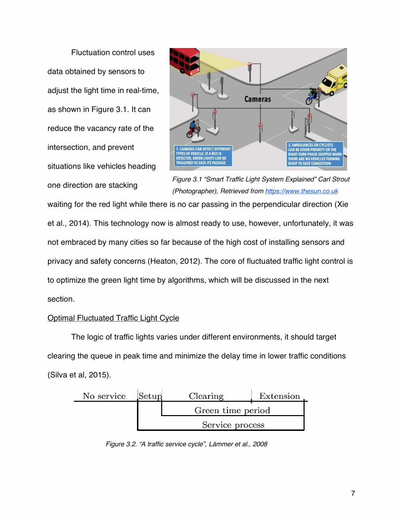
Fluctuation control uses

data obtained by sensors to

adjust the light time in real-time,

as shown in Figure 3.1. It can

reduce the vacancy rate of the

intersection, and prevent

situations like vehicles heading

one direction are stacking

waiting for the red light while there is no car passing in the perpendicular direction (Xie

et al., 2014). This technology now is almost ready to use, however, unfortunately, it was

not embraced by many cities so far because of the high cost of installing sensors and

privacy and safety concerns (Heaton, 2012). The core of fluctuated traffic light control is

to optimize the green light time by algorithms, which will be discussed in the next

section.

Optimal Fluctuated Traffic Light Cycle

The logic of traffic lights varies under different environments, it should target

clearing the queue in peak time and minimize the delay time in lower traffic conditions

(Silva et al, 2015).

Figure 3.1 “Smart Traffic Light System Explained” Carl Strout (Photographer), Retrieved from https://www.thesun.co.uk

Figure 3.2. “A traffic service cycle”, Lämmer et al., 2008

8

As depicted in Figure 3.2, the green light service process can be divided into

three phases: set-up, clearing, and extension. The set-up time stands for all time losses

associated with the start of green light service, including yellow light time, and time for

all corresponding vehicles, bikes, or pedestrians to leave the conflict area, which usually

lies between 3 and 8 seconds (Lämmer et al., 2008). The clearing phase reflects the

time needed to clear the queue accumulated during no service period and incoming

vehicles during the clearing phase; free flow reached indicates the start of the extension

period, the lights remain green for a short time to the end of the green light service.

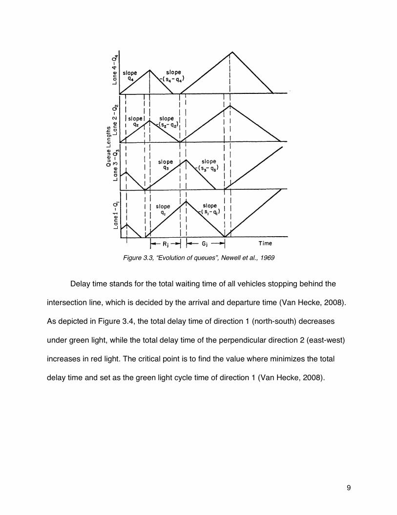
The time needed to clear a queue varies from intersection to intersection based

on the different lane numbers, driving behaviors, directions, and so on (Newell et al.,

1969). For a typical four-directional intersection, the queue length and time can be

shown in Figure 3.3. Lane 1 and 3 are lanes heading opposite directions perpendicular

to lane 2 and 4. The slope of the upward line segments can be calculated from vehicle

volume. In contrast, the downward line segment slope is decided by the speed of

vehicles leaving the intersection and the incoming vehicle volume (Newell, 1969).

9

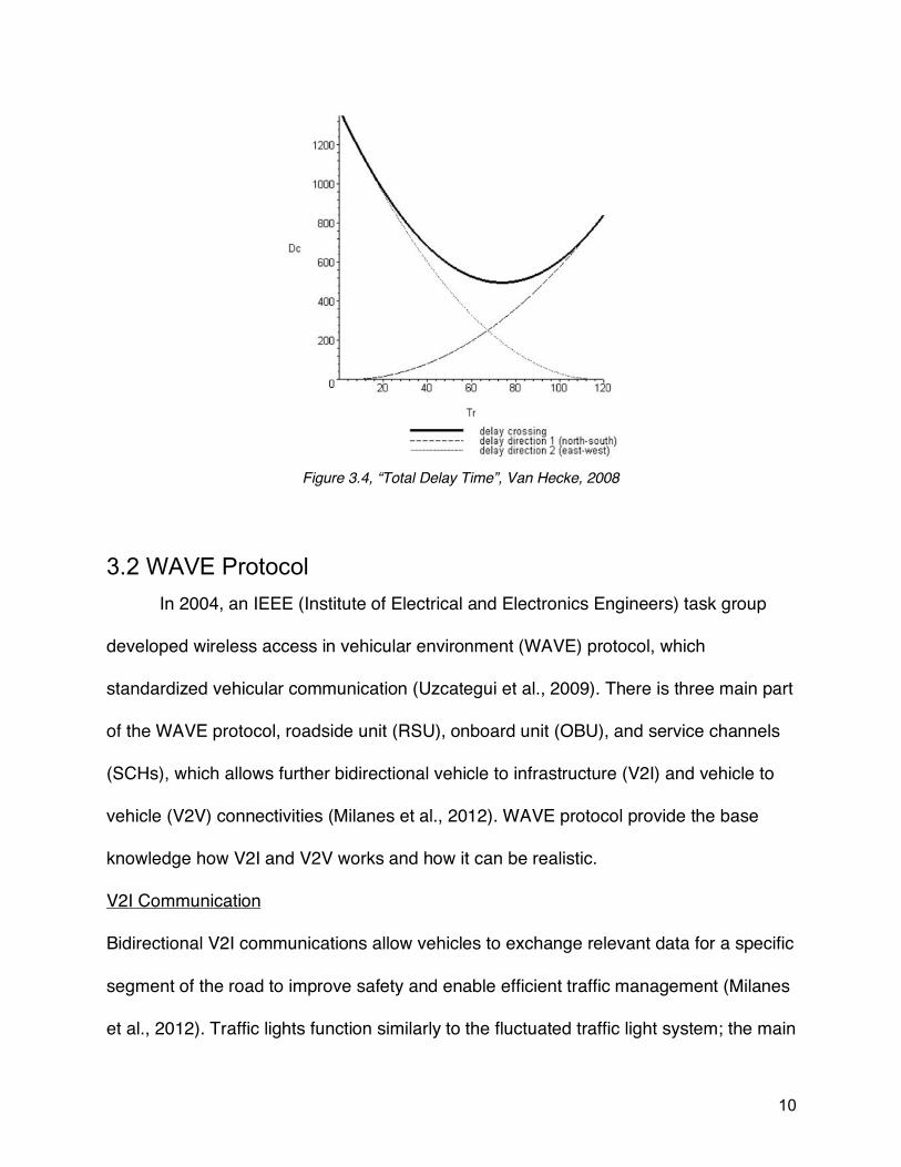
Delay time stands for the total waiting time of all vehicles stopping behind the

intersection line, which is decided by the arrival and departure time (Van Hecke, 2008).

As depicted in Figure 3.4, the total delay time of direction 1 (north-south) decreases

under green light, while the total delay time of the perpendicular direction 2 (east-west)

increases in red light. The critical point is to find the value where minimizes the total

delay time and set as the green light cycle time of direction 1 (Van Hecke, 2008).

Figure 3.3, “Evolution of queues”, Newell et al., 1969

10

3.2 WAVE Protocol In 2004, an IEEE (Institute of Electrical and Electronics Engineers) task group

developed wireless access in vehicular environment (WAVE) protocol, which

standardized vehicular communication (Uzcategui et al., 2009). There is three main part

of the WAVE protocol, roadside unit (RSU), onboard unit (OBU), and service channels

(SCHs), which allows further bidirectional vehicle to infrastructure (V2I) and vehicle to

vehicle (V2V) connectivities (Milanes et al., 2012). WAVE protocol provide the base

knowledge how V2I and V2V works and how it can be realistic.

V2I Communication

Bidirectional V2I communications allow vehicles to exchange relevant data for a specific

segment of the road to improve safety and enable efficient traffic management (Milanes

et al., 2012). Traffic lights function similarly to the fluctuated traffic light system; the main

Figure 3.4, “Total Delay Time”, Van Hecke, 2008

11

difference is the source of information; instead of sensors, the traffic information is

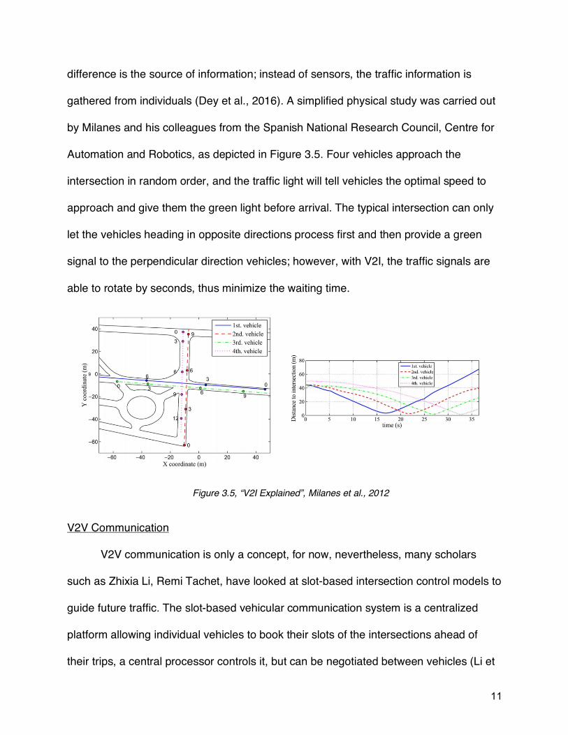
gathered from individuals (Dey et al., 2016). A simplified physical study was carried out

by Milanes and his colleagues from the Spanish National Research Council, Centre for

Automation and Robotics, as depicted in Figure 3.5. Four vehicles approach the

intersection in random order, and the traffic light will tell vehicles the optimal speed to

approach and give them the green light before arrival. The typical intersection can only

let the vehicles heading in opposite directions process first and then provide a green

signal to the perpendicular direction vehicles; however, with V2I, the traffic signals are

able to rotate by seconds, thus minimize the waiting time.

V2V Communication

V2V communication is only a concept, for now, nevertheless, many scholars

such as Zhixia Li, Remi Tachet, have looked at slot-based intersection control models to

guide future traffic. The slot-based vehicular communication system is a centralized

platform allowing individual vehicles to book their slots of the intersections ahead of

their trips, a central processor controls it, but can be negotiated between vehicles (Li et

Figure 3.5, “V2I Explained”, Milanes et al., 2012

12

al., 2013). Interestingly, Li’s group chose to use the delay time as the criteria, while

Tachet’s group chose intersection capacity as their criteria.

Li used a first-come-first-serve protocol named autonomous control of urban

traffic (ACUTA) to guide the intersection operation system. Under ACUTA, each

approaching vehicle sets up a communication connection with the intersection control

center, which is named IM, after it enters IM’s range. IM will get the full information of

the vehicle, including location, speed, maximum acceleration and deceleration rate,

routing information, and then calculate the possible crossing time of one vehicle. The

calculation is based on the acceleration and deceleration rate, for acceleration rate !":

a!" = !%&' − (* − 1)-%!%&'

where

a* = ./01/23/2145/6

a!" = *7ℎ9:..*5;/!;7/62!7*</!33/;/6!7*:26!7/,

a!%&' = 4!=*414!33/;/6!7*:26!7/, !2?

a4 = 7ℎ/4!=*4142145/6:@*27/62!;.*41;!7*:2.!;;:A/?5B7ℎ/CD

If all available slots are booked, IM will reject the request temporarily and give the

vehicle a deceleration rate in a similar process of acceleration. If IM approves a

reservation request, it will send an approval message to the requesting vehicle along

with a designated acceleration rate, which will result in no conflicts with existing

reservations.

The results of Li’s study are shown in Figure 3.6, ACUTA intersection, and

traditional signaled intersection performed similarly under low traffic and extremely high

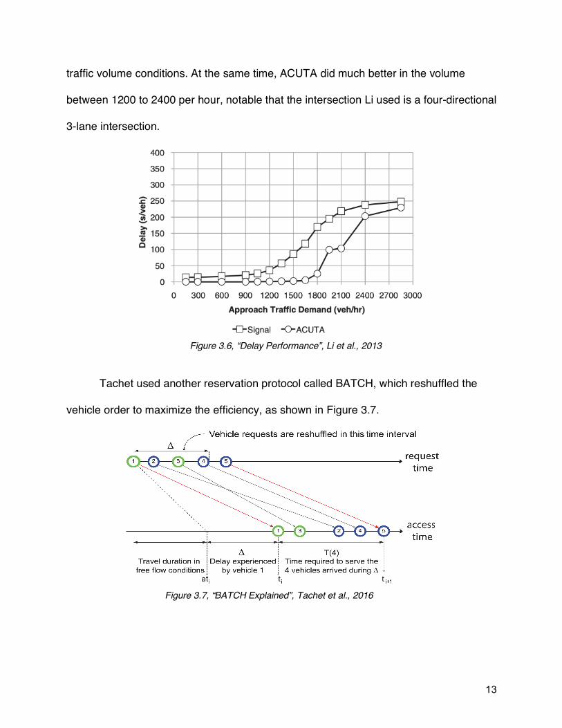
13

traffic volume conditions. At the same time, ACUTA did much better in the volume

between 1200 to 2400 per hour, notable that the intersection Li used is a four-directional

3-lane intersection.

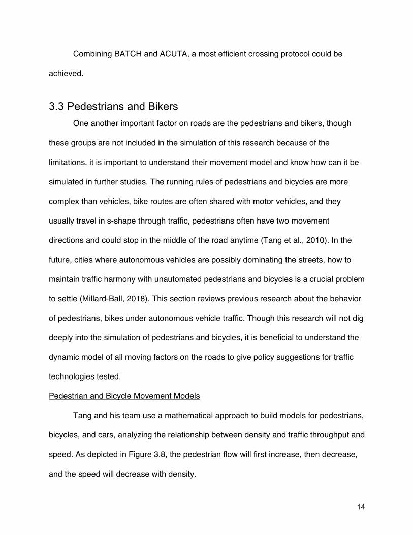
Tachet used another reservation protocol called BATCH, which reshuffled the

vehicle order to maximize the efficiency, as shown in Figure 3.7.

Figure 3.6, “Delay Performance”, Li et al., 2013

Figure 3.7, “BATCH Explained”, Tachet et al., 2016

14

Combining BATCH and ACUTA, a most efficient crossing protocol could be

achieved.

3.3 Pedestrians and Bikers One another important factor on roads are the pedestrians and bikers, though

these groups are not included in the simulation of this research because of the

limitations, it is important to understand their movement model and know how can it be

simulated in further studies. The running rules of pedestrians and bicycles are more

complex than vehicles, bike routes are often shared with motor vehicles, and they

usually travel in s-shape through traffic, pedestrians often have two movement

directions and could stop in the middle of the road anytime (Tang et al., 2010). In the

future, cities where autonomous vehicles are possibly dominating the streets, how to

maintain traffic harmony with unautomated pedestrians and bicycles is a crucial problem

to settle (Millard-Ball, 2018). This section reviews previous research about the behavior

of pedestrians, bikes under autonomous vehicle traffic. Though this research will not dig

deeply into the simulation of pedestrians and bicycles, it is beneficial to understand the

dynamic model of all moving factors on the roads to give policy suggestions for traffic

technologies tested.

Pedestrian and Bicycle Movement Models

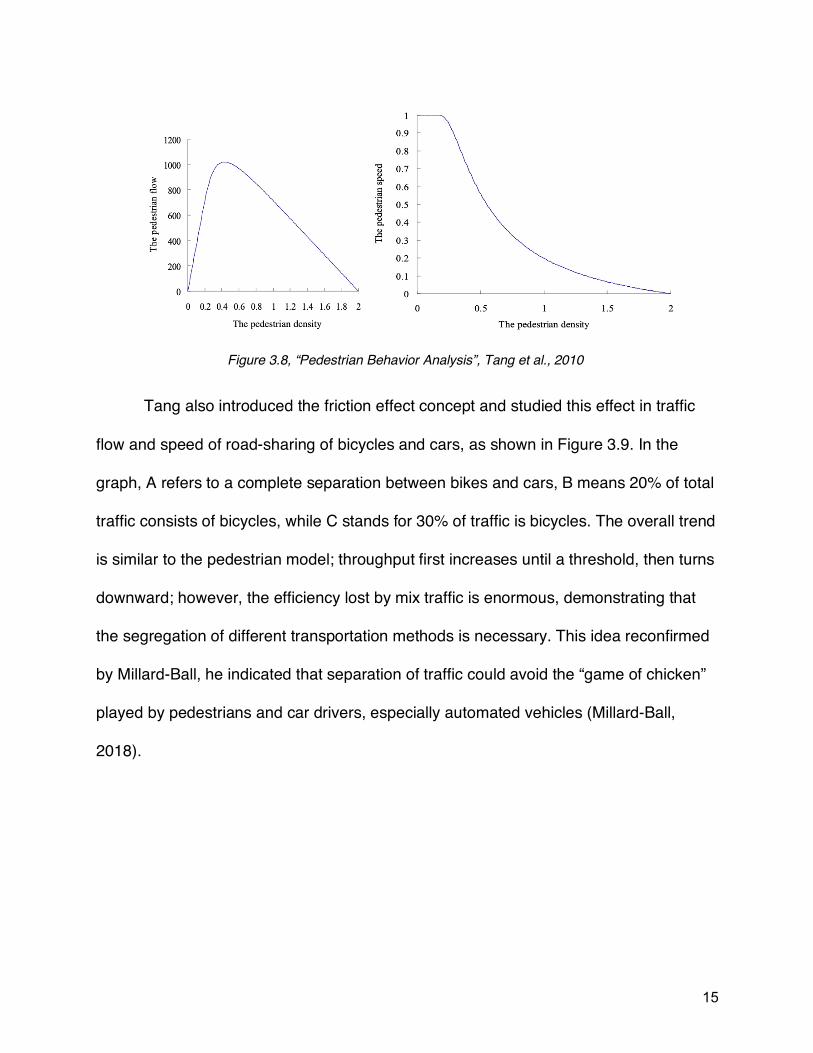
Tang and his team use a mathematical approach to build models for pedestrians,

bicycles, and cars, analyzing the relationship between density and traffic throughput and

speed. As depicted in Figure 3.8, the pedestrian flow will first increase, then decrease,

and the speed will decrease with density.

15

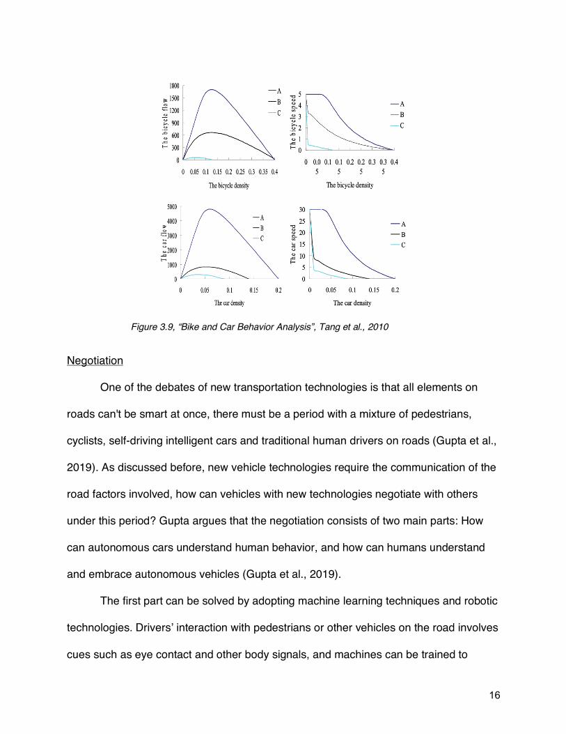
Tang also introduced the friction effect concept and studied this effect in traffic

flow and speed of road-sharing of bicycles and cars, as shown in Figure 3.9. In the

graph, A refers to a complete separation between bikes and cars, B means 20% of total

traffic consists of bicycles, while C stands for 30% of traffic is bicycles. The overall trend

is similar to the pedestrian model; throughput first increases until a threshold, then turns

downward; however, the efficiency lost by mix traffic is enormous, demonstrating that

the segregation of different transportation methods is necessary. This idea reconfirmed

by Millard-Ball, he indicated that separation of traffic could avoid the “game of chicken”

played by pedestrians and car drivers, especially automated vehicles (Millard-Ball,

2018).

Figure 3.8, “Pedestrian Behavior Analysis”, Tang et al., 2010

16

Negotiation

One of the debates of new transportation technologies is that all elements on

roads can't be smart at once, there must be a period with a mixture of pedestrians,

cyclists, self-driving intelligent cars and traditional human drivers on roads (Gupta et al.,

2019). As discussed before, new vehicle technologies require the communication of the

road factors involved, how can vehicles with new technologies negotiate with others

under this period? Gupta argues that the negotiation consists of two main parts: How

can autonomous cars understand human behavior, and how can humans understand

and embrace autonomous vehicles (Gupta et al., 2019).

The first part can be solved by adopting machine learning techniques and robotic

technologies. Drivers’ interaction with pedestrians or other vehicles on the road involves

cues such as eye contact and other body signals, and machines can be trained to

Figure 3.9, “Bike and Car Behavior Analysis”, Tang et al., 2010

17

understand gestures and even generate information from facial expressions (Han et al.,

2013). The key question is whether machines can decode and react to dynamic cues

from the real environment (Gupta et al., 2019).

3.4 Greenhouse Gases (GHG) Emission from Transportation According to the United States Environmental Protection Agency (EPA), 30% of

total GHG emission across the nation is generated by transportation, and over 90

percent of the fuel used for transportation is petroleum based, which includes primarily

gasoline and diesel (2019). GHG emission is one of the most important drawbacks of

using personal vehicles, however, reduce the travel time and car idling time can

improve the GHG emission performance. This part of literature means to provide a

model to calculate the GHG reduction by different technologies. The total GHG

emission in the intersection is related to (Jung et al, 2011):

a) Vehicle speed

b) Distance traveled

c) Time

d) Road surface condition and slope

The distance traveled in the intersection is almost constant, the road surface and

slope can be set as unchanged, it becomes a relationship with speed and travel time.

Jiménez-Palacios (1999) in his research build a formula calculating GHG Emission by

equation:

aE4*..*:2 = < × (1.1! + 0.132) + 0.000302 × <L

where:

18

a< = </ℎ*3;/.9//?(4/.)

a! = </ℎ*3;/!33/;/6!7*:26!7/(4/.N)

3.5 Intersection Performance Evaluation Various parameters are considered in the previous studies regarding traffic

performance. Hatami et al., Van Hecke et al., and Li et al. used delay time to reflect the

efficiency of the intersection. Delay time is measured from the time used to cross the

intersection under conditions minus the time used as free flow. It can be further

developed into average delay and total delay (Li et al., 2013). Hatami et al. and Techet

et al. used intersection capacity (throughput) as a performance indicator. Interestingly,

Anisimov et al. used time of inefficient operation as the criteria of traffic performance,

which is measured by the accumulated unnecessary wait time of the vehicles (i.e.,

vehicles from south to north wait for the red light while no car is traveling from

perpendicular directions). Moreover, Tang et al. and Milanes et al. used vehicle speed,

Bani Younes et al. used road density, Kerimov et al. used the number of traffic

accidents to present the traffic performance.

19

Chapter 4: Methodology

4.1 Study Site Selection The intersection of Queen Street crossing Spadina Avenue in downtown Toronto

is picked to be the research intersection.

Located on the north shore of

the Lake of Ontario, the Canadian

city of Toronto inhabited with 2.73

million population (Statistics Canada,

2016), makes it the largest city in

Canada, as well as the fourth largest

city in North America. Similar to other

American metropolises, private

vehicles dominate people’s

commuting methods. Among the

1.25 million employed labor force aged 15 years and over with a usual place of work,

more than half of them commute in personal vehicles, and merely 23.3% of them travel

by public transits (Statistics Canada, 2011), this number in New York central business

areas is nearly 80% (MTA, 2019), not to mention the commuters live in the suburb

areas. Domination of car travel drives Toronto to the sixth place of the most congested

cities in North America according to the Tomtom Traffic Index, and the average travel

time is 32% more than the travel time in the designed speed, the same number of New

York City is 36% (Tomtom, 2018). Moreover, the part of King’s Highway 401, which

Figure 4.1 “Location of Toronto” SimonP (Photographer), Retrieved from https://commons.wikimedia.org/

The red area shows Toronto’s location on the north shore of Lake Ontario.

20

passes through the city is North America’s busiest highway, around half a million

vehicles travel on it in every typical day (Maier, 2007). The lousy traffic condition,

together with Toronto’s Greenhouse Gas Emission goals, drew scholars’ and officials’

attention to the transformation of transportation in the city.

King Street and Queen Street are two major east-west thoroughfares in

downtown Toronto, in November 2017, the city council launched the pilot transit priority

corridor project, which put pedestrian and transit first through improved transit reliability,

speed, and capacity. The trial of over a year proved that people are moved more

efficiently in transit without compromising the road network. In April 2019, King Street is

announced to be a permanent transit priority corridor (City of Toronto, 2019). Three

blocks north, Queen Street is relatively quiet in the transformation period of King Street,

which in other words, is waiting for the changes. The problems these two streets facing

are similar: narrow streets, large volumes, and numerous means of transportation.

There is nowadays a debate between promoting public transit or staying with personal

vehicles. Comparing the results of this research and the results from the King Street

Public Transit Corridor project, the readers could get some evidence of whether the new

technologies may change the current debate.

21

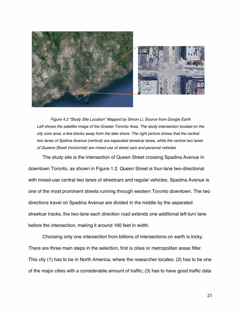
The study site is the intersection of Queen Street crossing Spadina Avenue in

downtown Toronto, as shown in Figure 1.2. Queen Street is four-lane two-directional

with mixed-use central two lanes of streetcars and regular vehicles. Spadina Avenue is

one of the most prominent streets running through western Toronto downtown. The two

directions travel on Spadina Avenue are divided in the middle by the separated

streetcar tracks, the two-lane each direction road extends one additional left-turn lane

before the intersection, making it around 160 feet in width.

Choosing only one intersection from billions of intersections on earth is tricky.

There are three main steps in the selection, first is cities or metropolitan areas filter.

This city (1) has to be in North America, where the researcher locates; (2) has to be one

of the major cities with a considerable amount of traffic; (3) has to have good traffic data

Figure 4.2 “Study Site Location” Mapped by Simon Li, Source from Google Earth Left shows the satellite image of the Greater Toronto Area. The study intersection located on the city core area, a few blocks away from the lake shore. The right picture shows that the central two lanes of Spidina Avenue (vertical) are separated streetcar lanes, while the central two lanes of Queens Street (horizontal) are mixed use of street cars and personal vehicles

22

transparency and availability; (4) is suffering from congestion and eager to change. The

main purpose of setting these criteria is to make the research authentic and meaningful.

After setting the filter, four cities stand out, which are New York City, NY; Boston, MA;

San Francisco, CA, and Toronto, Canada.

A detailed examination then carried out to pick the most suitable city from four

candidates. Toronto performs best in this part. Firstly, the road situation in Toronto is

complicated. Not only cars and bikes run on the streets, but also trains which are called

the Toronto Streetcar System. Though San Francisco also has its own cable car

system, it is more like a historical site and not many people use it as daily transit

(SFMTA, 2020). Moreover, the streetcar network in Toronto is more complete with 10

lines and 685 stops carrying nearly 500,000 ridership on a normal workday (TTC, 2019).

Secondly, Toronto has very detailed traffic data of all major and some of the minor

intersections in the downtown area. The data interval is fifteen minutes, and it includes

not only vehicle counts and directions, but also pedestrians, bikes, buses, freight trucks,

and most importantly, streetcars. And thirdly, Toronto is suffering from congestion and

enthusiastic about new changes. As stated before, Toronto ranked the top ten most

congested cities in North America, and they tried many methods to make the situation

better including creating public transit corridors (City of Toronto, 2019).

To Finalize the only intersection from thousands of intersections in Toronto,

some more criteria are set. The intersection (1) has to have entire data coverage

throughout the year; (2) has to have multiple lanes; (3) has to involve vehicles,

streetcars, bikes, and pedestrians; (4) has to have an apparent peak and valley shaped

23

traffic count during a day; (5) with a streetcar stop near the intersection is a plus. The

main purpose of setting these criteria is to pick a study site with a complicated situation

that is hard for a human being to get an optimal solution easily, thus can test the

potential of new technologies. The intersection of Queen Street crossing Spadina

Avenue was finally selected as the study intersection. Moreover, this site also has a

great value to expand the research results to other intersections with its normality as a

two-lane traffic intersection, as well as its complexity as a mix of all road factors.

4.2 Initial Data Research Before starting the simulation building, an initial data research to check data

quality, as well as get baseline information about the study site was carried out. All

traffic data are fetched from Toronto Open Data.

Fluctuation Throughout One Typical Day

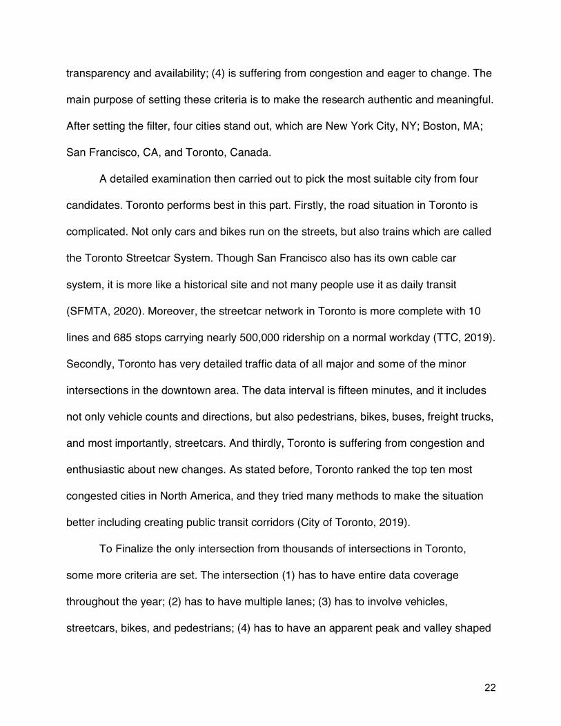
The traffic of the study intersection is not stable throughout one typical day, and it

has two peaks, one in the morning at around 8:30 a.m., another one in the evening at

around 6:00 p.m. The peak volume is about 1300 vehicles per hour. During the daytime,

the intersection is busy most of the time, with the lowest quantity of 988 vehicles per

hour occurring at 11:00 a.m. At night, the intersection remains silent, reaching its lowest

point of 167 vehicles passing from 4:45 to 5:45 a.m. This data research reveals that the

intersection is under tremendous traffic pressure in the daytime, where the maximizing

total throughput should be the primary target, and delay time should be minimized from

11:00 p.m. to 7:30 a.m. (Lämmer et al. 2008).

24

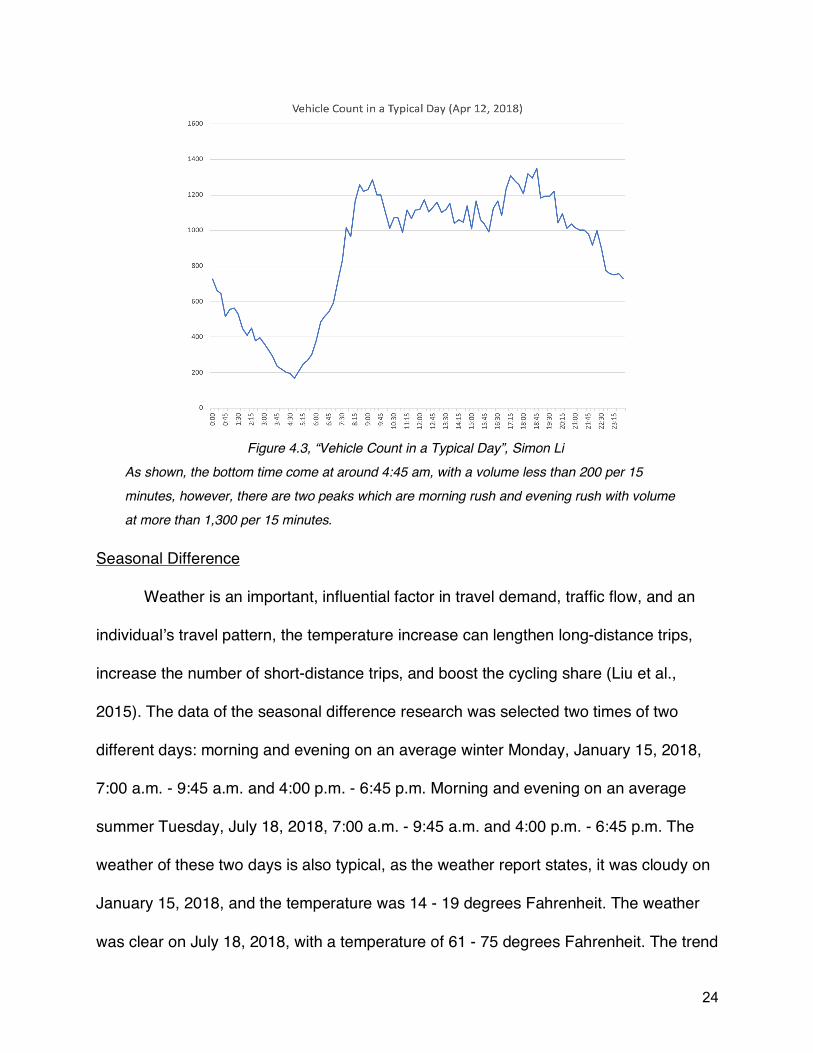
Seasonal Difference

Weather is an important, influential factor in travel demand, traffic flow, and an

individual’s travel pattern, the temperature increase can lengthen long-distance trips,

increase the number of short-distance trips, and boost the cycling share (Liu et al.,

2015). The data of the seasonal difference research was selected two times of two

different days: morning and evening on an average winter Monday, January 15, 2018,

7:00 a.m. - 9:45 a.m. and 4:00 p.m. - 6:45 p.m. Morning and evening on an average

summer Tuesday, July 18, 2018, 7:00 a.m. - 9:45 a.m. and 4:00 p.m. - 6:45 p.m. The

weather of these two days is also typical, as the weather report states, it was cloudy on

January 15, 2018, and the temperature was 14 - 19 degrees Fahrenheit. The weather

was clear on July 18, 2018, with a temperature of 61 - 75 degrees Fahrenheit. The trend

Figure 4.3, “Vehicle Count in a Typical Day”, Simon Li As shown, the bottom time come at around 4:45 am, with a volume less than 200 per 15 minutes, however, there are two peaks which are morning rush and evening rush with volume at more than 1,300 per 15 minutes.

25

of vehicles passing through the crossing is similar in summer and winter; however, it is

apparent that the summer evening volume is higher than any other times and there is a

continuous upward trend in the summer evening after 6:30 p.m., which indicates that

people tend to be out more often and later in summer times. Different from my

prefiguration, people in downtown Toronto only drive a little bit more in wintertime. In

total, 12,214 cars traveled across the intersection in the winter morning, only 186 more

than that in the summer morning. As for the pedestrians, the contrast of seasons is

more prominent, and the pedestrians count in the fifteen minutes time frame after 5:00

p.m. on July 18 marked the peak of the counted time with 1514 people gone across.

Figure 4.4, “Seasonal Difference”, Simon Li

During Summer time, the personal vehicle count is generally lower than that in winter time. More people in summer walk, use public transits or bikes to commute.

26

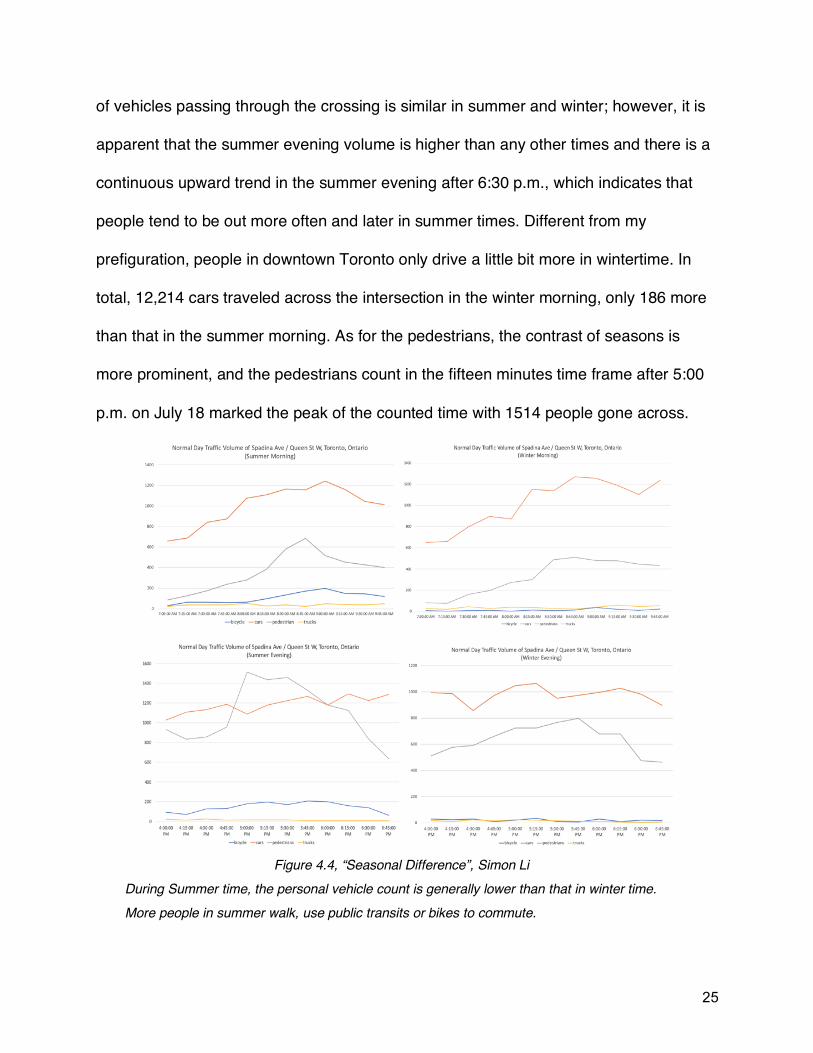
Biking

There is a designed bicycle lane along Spadina Street; however, bicycles have

no priority and need to compete with motorized vehicles along Queen Street. Though

bike share in downtown Toronto is well designed, the harsh winter weather and bicycle-

unfriendly street services keep the ride numbers low, especially in wintertime. As

depicted in Figure 4.5, the seasonal difference in biking is dramatic, and this is in the

clear weather, I believe the number will be almost flat zero on snowy days.

4.3 Simulation There are four simulation scenarios performed in the research, as demonstrated

in Table 4.1.

Figure 4.5, “Bicycle Contrast”, Simon Li Seasonal difference of bikers count between winter and summer is huge, as the blue line showing winter situation and orange line showing summer situation

27

Scenario Index

Technology Involved Hardware Involved Precedent

Requirements Vehicle Behavior Lane Behavior

0 Status Quo

• Normal vehicles, • Traditional traffic light, • Physical lane markers

and signs

N/A Manual Central lane for left turn and straight, right lane for right and straight

1 Intelligent Traffic Light

• Normal vehicles, • Traditional traffic light

with sensor, • Physical lane markers

and signs,

Sensors availability Manual Central lane for left turn and straight, right lane for right and straight

2 V2I Communication

• Vehicles with Communication antenna and advanced driving assistant software installed,

• Traffic light with communicational control system

• Physical and digital lane markers and signs

High-speed communication network

On-board computer will inform drivers road information, optimized vehicles speed, and designated lane

Lanes will be assigned by intersection central control for drivers to follow

3 V2V Communication

• Autonomous vehicles • Virtual traffic light • Virtual lane markers and

signs

Stable & high-speed communication network, Autonomous vehicles,

Completely autonomous vehicles, human only act as passengers

Lanes will be assigned to vehicles

Table 4.1, “Scenario Description”, Simon Li

28

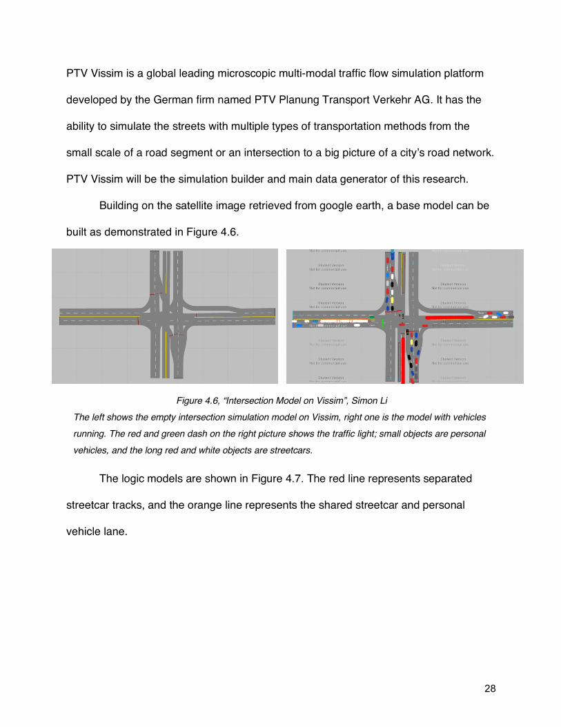
PTV Vissim is a global leading microscopic multi-modal traffic flow simulation platform

developed by the German firm named PTV Planung Transport Verkehr AG. It has the

ability to simulate the streets with multiple types of transportation methods from the

small scale of a road segment or an intersection to a big picture of a city’s road network.

PTV Vissim will be the simulation builder and main data generator of this research.

Building on the satellite image retrieved from google earth, a base model can be

built as demonstrated in Figure 4.6.

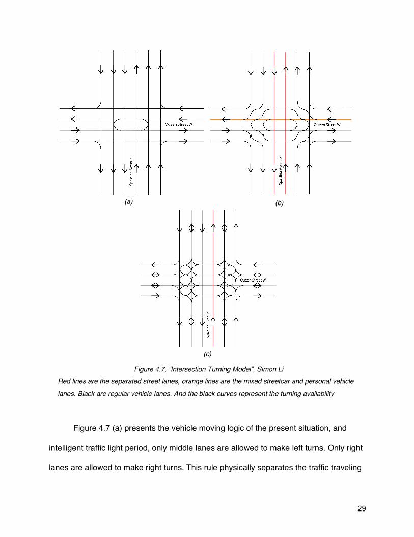
The logic models are shown in Figure 4.7. The red line represents separated

streetcar tracks, and the orange line represents the shared streetcar and personal

vehicle lane.

Figure 4.6, “Intersection Model on Vissim”, Simon Li The left shows the empty intersection simulation model on Vissim, right one is the model with vehicles running. The red and green dash on the right picture shows the traffic light; small objects are personal vehicles, and the long red and white objects are streetcars.

29

Figure 4.7 (a) presents the vehicle moving logic of the present situation, and

intelligent traffic light period, only middle lanes are allowed to make left turns. Only right

lanes are allowed to make right turns. This rule physically separates the traffic traveling

Figure 4.7, “Intersection Turning Model”, Simon Li Red lines are the separated street lanes, orange lines are the mixed streetcar and personal vehicle lanes. Black are regular vehicle lanes. And the black curves represent the turning availability

(a)

(b)

(c)

30

different directions, thus maintains the order and smoothness of traffic flow. However,

with technology evolvement, road traffic logic will change, as Figure 4.7 (b)

demonstrated, vehicles’ turning will not be limited to lanes anymore, traffic heading

different directions will be separated by time approaching the intersection. Under V2I

communication circumstance, the intersection command center will arrange the slots

allowing vehicles with similar routes approaching intersections to turn in different

directions using all lanes available to maximum capacity. Even more advanced, the

designated lane directions can be changed under demand, as shown in Figure 4.7 (c).

After having road models, traffic data and technology information are fitted into

models. Since the main purpose of the research is to demonstrate the technology

performance, all tunings will be based on the traffic data of April 12, 2018, which will not

autonomously adapt to different real-world situations, and may not reflect the exact

current traffic condition. Moreover, the traffic data is counted per fifteen minutes, the

distribution of vehicles arriving at the intersection are considered evenly during the

fifteen-minute time frame.

Scenario 0: Status Quo

In order to demonstrate the performance under both peak and bottom traffic

situations, a higher volume time period (6:45 p.m. - 7:00 p.m., April 12, 2018) and a

lower volume time period (6:00 a.m. - 6:15 a.m., April 12, 2018) are chosen to provide

the baseline data as shown in Table 4.2

31

Time Approach from East

Approach from North

Approach from South

Approach from West

NB&SB WB EB&WB SB EB&WB NB NB&SB EB

6:00 - 6:15 am 50 29 63 45 77 49 39 28

6:45 - 7:00 pm 170 151 209 150 235 136 139 160

Current traffic signal cycle is shown in Figure 4.8.

Scenario 1: Intelligent Traffic Light

Similar to scenario 0, there will be two sub-model simulating the high and low

traffic volume situations. The ratio of green light time regarding different directions is

calculated by equation:

!"1:!"2: . . . = )*1: )*2: . ..

where

!"1 = !+,,-"./,012.+,*".0-#1

!"2 = !+,,-"./,012.+,*".0-#2

...

Table 4.2, “Study Time Frame”, Simon Li

Figure 4.8, “Current Traffic Signal Cycle”, Simon Li The current cycle uses 120 seconds as one cycle, with 69 seconds north-south passing time and 51 seconds east-west passing time.

32

)*1 = ),ℎ.*5,*06-"012.+,*".0-#1

)*2 = ),ℎ.*5,*06-"012.+,*".0-#2

…

Based on the data and calculation, the ratio can be expressed by the equation:

For the bottom time:

5!7,: !7,: 5!-8: !-8 = 1: 1.27: 1.56: 2.09

For the peak time:

5!7,: !7,: 5!-8: !-8 = 1: 2.01: 1.44: 1.85

where

5!7, = 7,8",@8"2.+,*".0-5,1""6+-!+,,-"./,

!7, = 7,8",@8"2.+,*".0-!+,,-"./,

5!-8 = -0+"ℎ7,8"2.+,*".0-5,1""6+-!+,,-"./,

!-8 = -0+"ℎ7,8"2.+,*".0-!+,,-"./,

Take the ratio into simulation, the intersection performance changes by adjusting

the cycle length.

Scenario 2: V2I Communication

V2I enables intersection control centers to adjust the speed of approaching

vehicles and allow the clustering of vehicles traveling the same direction. Again, this

research does not mean to address how this technology functions in a real-world

situation; the simulation will assume that vehicles have already clustered by their

traveling direction before getting to the intersection zone. The light time ratio will remain

the same from scenario one since the vehicle number in the simulation remains

unchanged; the independent variable is still the cycle time.

33

Scenario 3: V2V Communication

Ideally, there will be no traffic waiting behind the line; all of the vehicles arrive

and enter the intersection without any delay. The simulation of this scenario assumes

that vehicles have already booked their slot of crossing the intersection beforehand, and

will get through the intersection at a designed speed under the limit.

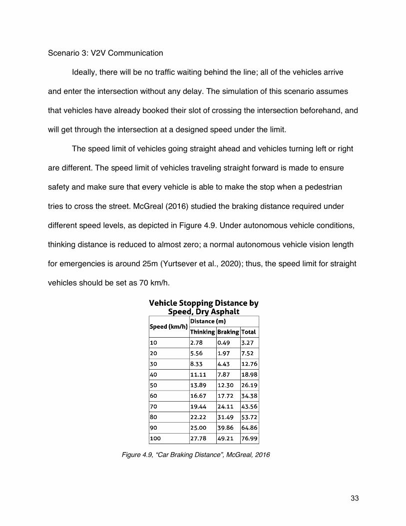
The speed limit of vehicles going straight ahead and vehicles turning left or right

are different. The speed limit of vehicles traveling straight forward is made to ensure

safety and make sure that every vehicle is able to make the stop when a pedestrian

tries to cross the street. McGreal (2016) studied the braking distance required under

different speed levels, as depicted in Figure 4.9. Under autonomous vehicle conditions,

thinking distance is reduced to almost zero; a normal autonomous vehicle vision length

for emergencies is around 25m (Yurtsever et al., 2020); thus, the speed limit for straight

vehicles should be set as 70 km/h.

Figure 4.9, “Car Braking Distance”, McGreal, 2016

34

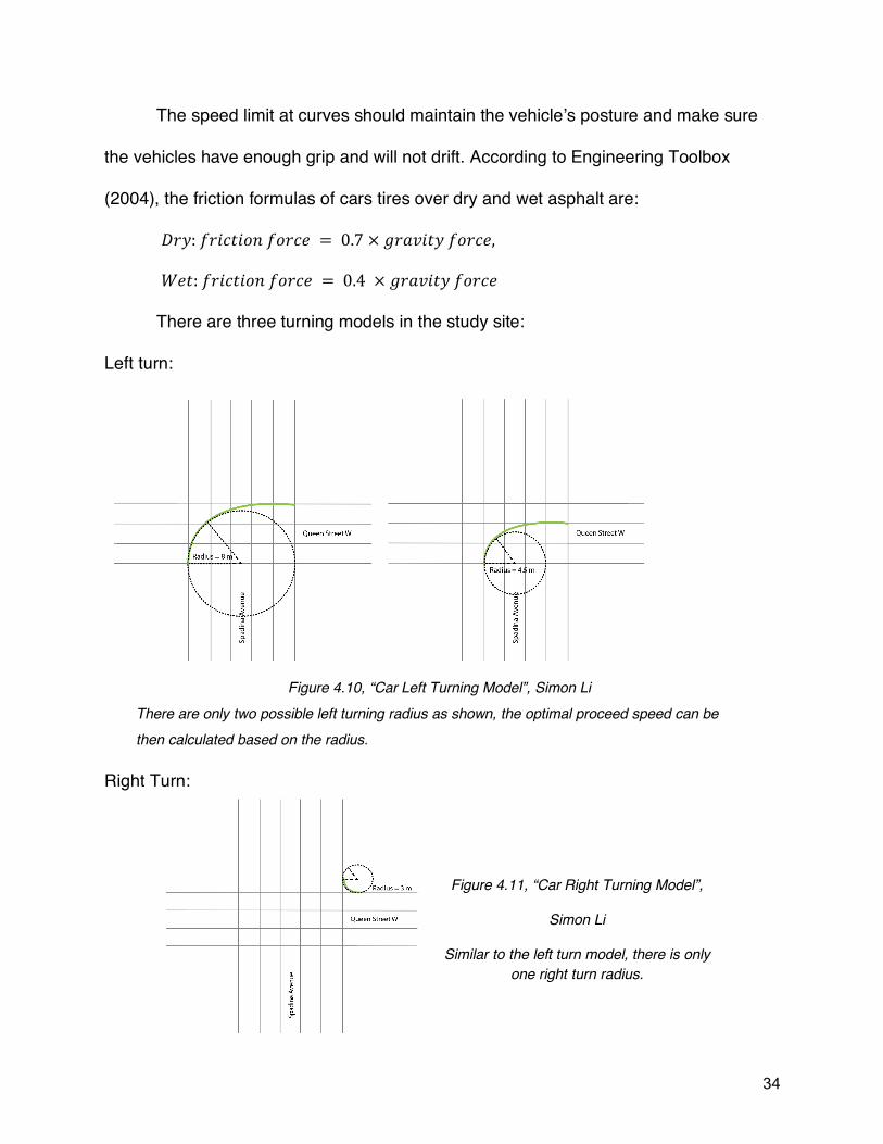
The speed limit at curves should maintain the vehicle’s posture and make sure

the vehicles have enough grip and will not drift. According to Engineering Toolbox

(2004), the friction formulas of cars tires over dry and wet asphalt are:

A+B:1+.*".0-10+*, = 0.7 × !+@)."B10+*,,

E,":1+.*".0-10+*, = 0.4 × !+@)."B10+*,

There are three turning models in the study site:

Left turn:

Right Turn:

Figure 4.11, “Car Right Turning Model”,

Simon Li

Similar to the left turn model, there is only one right turn radius.

Figure 4.10, “Car Left Turning Model”, Simon Li There are only two possible left turning radius as shown, the optimal proceed speed can be then calculated based on the radius.

35

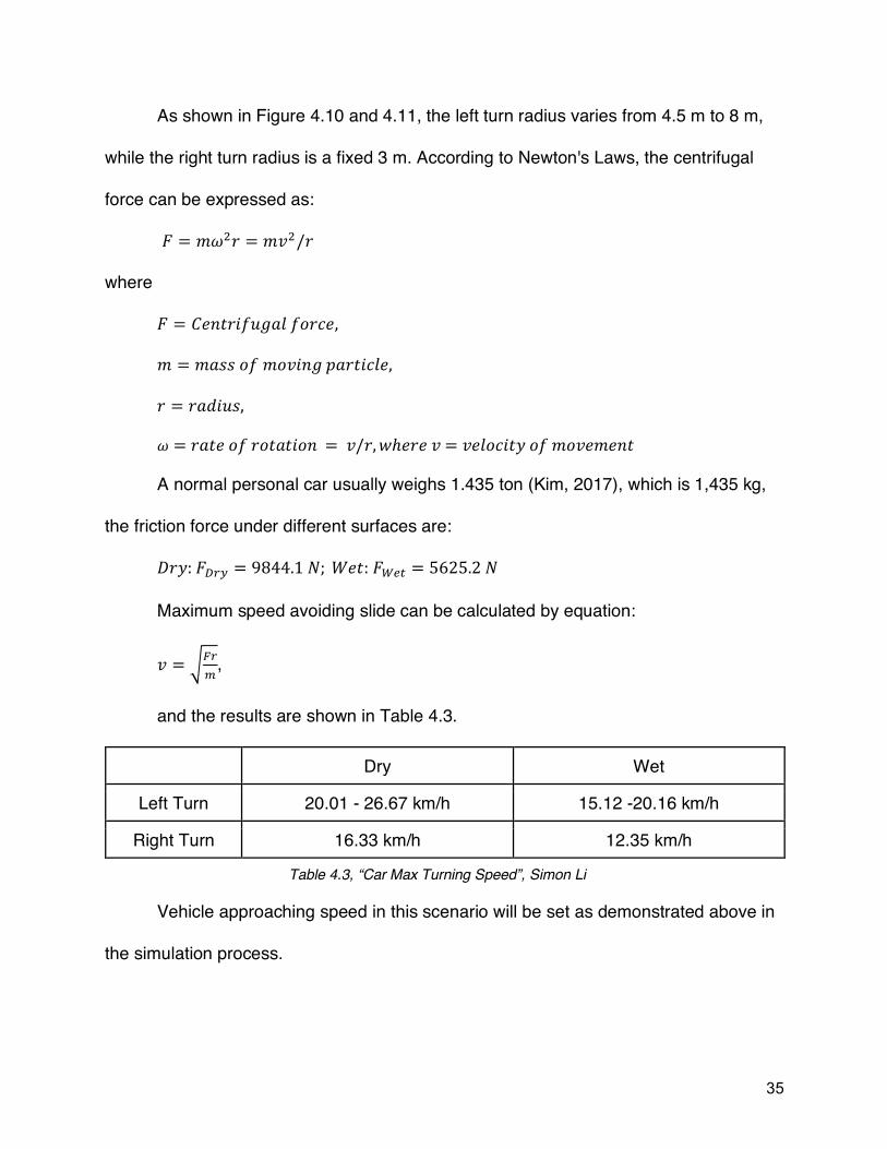
As shown in Figure 4.10 and 4.11, the left turn radius varies from 4.5 m to 8 m,

while the right turn radius is a fixed 3 m. According to Newton's Laws, the centrifugal

force can be expressed as:

F = /GH+ = /)H/+

where

F = J,-"+.16!@510+*,,

/ = /@8801/0).-!K@+".*5,,

+ = [email protected],

G = +@",01+0"@".0- = )/+,7ℎ,+,) = ),50*."B01/0),/,-"

A normal personal car usually weighs 1.435 ton (Kim, 2017), which is 1,435 kg,

the friction force under different surfaces are:

A+B:FLMN = 9844.1O; E,":FQRS = 5625.2O

Maximum speed avoiding slide can be calculated by equation:

) = TUMV

,

and the results are shown in Table 4.3.

Dry Wet

Left Turn 20.01 - 26.67 km/h 15.12 -20.16 km/h

Right Turn 16.33 km/h 12.35 km/h

Vehicle approaching speed in this scenario will be set as demonstrated above in

the simulation process.

Table 4.3, “Car Max Turning Speed”, Simon Li

36

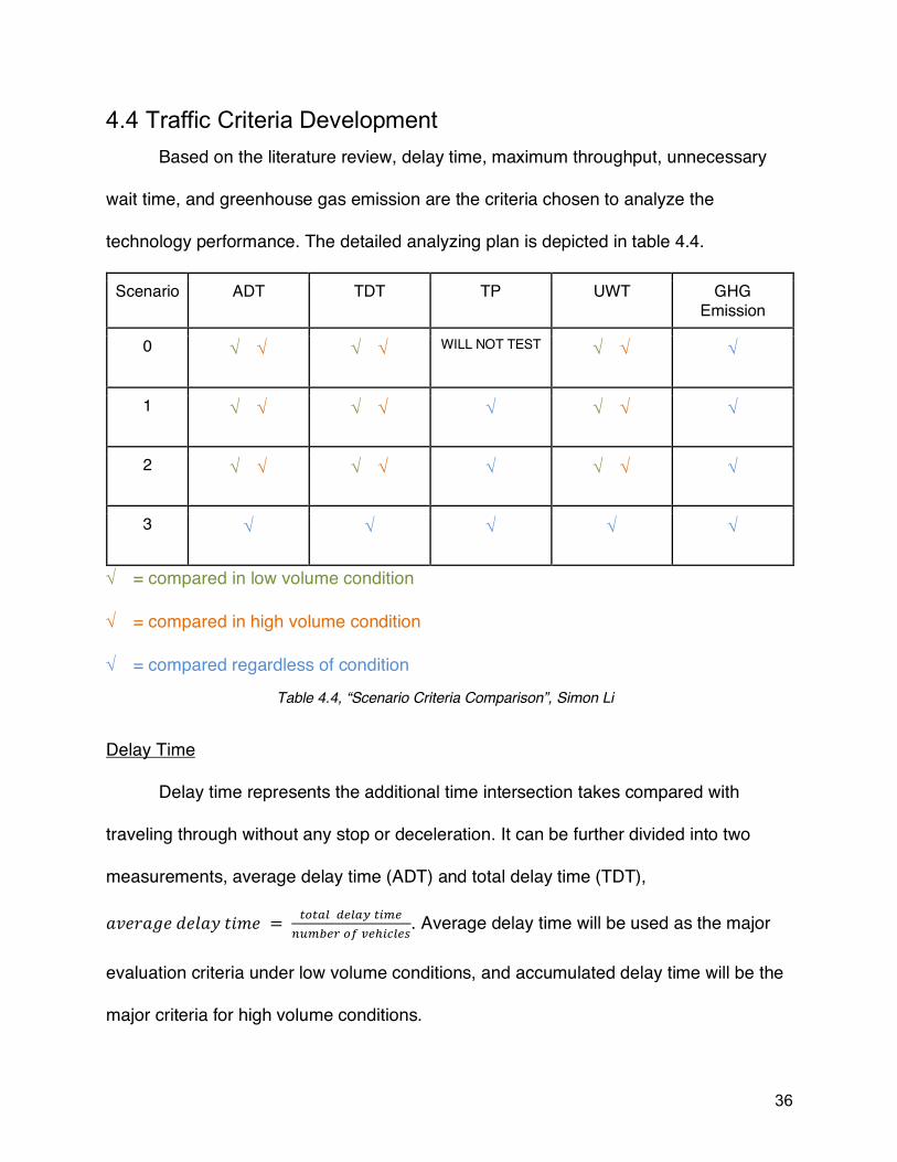
4.4 Traffic Criteria Development Based on the literature review, delay time, maximum throughput, unnecessary

wait time, and greenhouse gas emission are the criteria chosen to analyze the

technology performance. The detailed analyzing plan is depicted in table 4.4.

Scenario ADT TDT TP UWT GHG Emission

0 Ö Ö Ö Ö WILL NOT TEST Ö Ö Ö

1 Ö Ö Ö Ö Ö Ö Ö Ö

2 Ö Ö Ö Ö Ö Ö Ö Ö

3 Ö Ö Ö Ö Ö

Ö = compared in low volume condition

Ö = compared in high volume condition

Ö = compared regardless of condition

Delay Time

Delay time represents the additional time intersection takes compared with

traveling through without any stop or deceleration. It can be further divided into two

measurements, average delay time (ADT) and total delay time (TDT),

@),+@!,2,5@B"./, = SWSXYZRYXNS[VR\]V^RMW_`Ra[bYRc

. Average delay time will be used as the major

evaluation criteria under low volume conditions, and accumulated delay time will be the

major criteria for high volume conditions.

Table 4.4, “Scenario Criteria Comparison”, Simon Li

37

Unnecessary wait time is the accumulation of meaningless delay time. For

example, only two vehicles are approaching the intersection in opposite directions, and

they are both going to make a left turn. Usually, these two vehicles do not have to wait;

however, the one that arrives slightly later fails to use its indicators, and the earlier one

is made to remain in the middle of the intersection meaninglessly. This kind of delay

often happens because of inadequate information and can be reduced or even

eliminated by communication technologies.

The changing variable under scenario 1 and 2 is the traffic light cycle time, and

delay times will be calculated and compared with the current state as scenario 0.

Notably, scenario 0 is static, and the performance is analyzed based on the current

driving habits and a 120-second cycle, as shown in Figure 4.8. For scenario 3, the

independent variable is the number of vehicles in the intersection from 0 to its maximum

throughput.

Throughput (TP)

Throughput stands for the maximum amount of vehicle that the intersection

under specific technology is able to serve. The simulation variables will be similar to the

measurement of delay time. This criterion only means to test the ultimate limit of

technologies, and real traffic data will not be applied to the models.

In the analysis, all other variables are fixed to its optimum state under peak

volume, increase the number of vehicles approaching to infinity and count how many

vehicles can pass the intersection.

38

Greenhouse Gases Emission (GHG Emission)

Environmental concerns are one of the prevailing criticisms of road traffic. GHG

are discharged from personal vehicles from the burning of fossil fuels due to the engine

operation. EPA (2018) pointed out that Greenhouse Gas emission of a personal vehicle

is linear related to the gasoline or diesel it burns in its Green Vehicle Guidebook:

CO2 Emissions from a gallon of gasoline: 8,887 grams CO2/ gallon

CO2 Emissions from a gallon of diesel: 10,180 grams CO2/ gallon

The amount of fuel a vehicle burns is influenced by idle time, acceleration rate,

and velocity, as shown in the equation (Bifulco et al, 2015):

F6,5d6+-"K,+6-.""./, = 7.75 + 0.005)H + 6.42@

where

@ = @**,5,+@".0-+@",(//8H),

) = ),50*."B(//8)

The total fuel burnt can be then calculated by applying the formula to the time.

And the comparison of fuel burnt can reflect the emission condition directly.

39

Chapter 5: Results

5.1 Delays for Intelligent Traffic Lights After several tests, quantic functions and septic functions are chosen to fit bottom

situation and peak situation best respectively, and are used for curve fitting as shown in

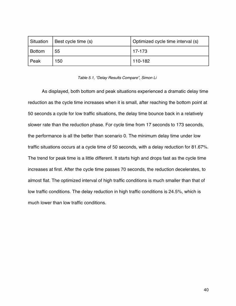
Figure 5.1. Table 5.1 displays the cycle length when minimum delay reached, and the

interval where delay time is less than that of scenario 0. Curves in UWT graphs are

fitted by using quantic functions, as shown in Figure 5.2.

Figure 5.1, “Intelligent Traffic Lights Delay Results”, Simon Li For the bottom situation, the delay time start high and reduce dramatically as the cycle time increase, reached the minimal point at the cycle of 55 seconds. The delay time rise again after this point almost linearly. As for the peak situation, the trend is similar, but with a wider low delay time range. Which stands that fluctuated traffic light have a better performance enhance under peak traffic situations.

40

As displayed, both bottom and peak situations experienced a dramatic delay time

reduction as the cycle time increases when it is small, after reaching the bottom point at

50 seconds a cycle for low traffic situations, the delay time bounce back in a relatively

slower rate than the reduction phase. For cycle time from 17 seconds to 173 seconds,

the performance is all the better than scenario 0. The minimum delay time under low

traffic situations occurs at a cycle time of 50 seconds, with a delay reduction for 81.67%.

The trend for peak time is a little different. It starts high and drops fast as the cycle time

increases at first. After the cycle time passes 70 seconds, the reduction decelerates, to

almost flat. The optimized interval of high traffic conditions is much smaller than that of

low traffic conditions. The delay reduction in high traffic conditions is 24.5%, which is

much lower than low traffic conditions.

Situation Best cycle time (s) Optimized cycle time interval (s)

Bottom 55 17-173

Peak 150 110-182

Table 5.1, “Delay Results Compare”, Simon Li

41

The trend of UWT and UWT percentage to total delay is similar, small in the

beginning and increases gradually until high. And the UWT of low traffic situations is

relatively higher than that of high traffic situations.

Figure 5.2, “Intelligent Traffic Lights UWT Results”, Simon Li For both bottom and peak situations, the unnecessary wait time remain low at first, then rising almost linearly. The percentage of UWT to total delay are S-shaped.

42

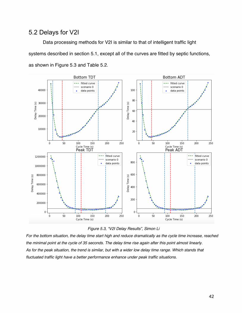
5.2 Delays for V2I Data processing methods for V2I is similar to that of intelligent traffic light

systems described in section 5.1, except all of the curves are fitted by septic functions,

as shown in Figure 5.3 and Table 5.2.

Figure 5.3, “V2I Delay Results”, Simon Li For the bottom situation, the delay time start high and reduce dramatically as the cycle time increase, reached the minimal point at the cycle of 35 seconds. The delay time rise again after this point almost linearly. As for the peak situation, the trend is similar, but with a wider low delay time range. Which stands that fluctuated traffic light have a better performance enhance under peak traffic situations.

43

Situation Best cycle time (s) Optimized cycle time interval (s)

Bottom 35 12-168

Peak 110 88-194

The overall trend of delay times in scenario 2 is similar to that in scenario 1,

except:

1. Under low traffic conditions, the minimum delay point occurs earlier.

2. The bottom part of the high traffic condition graphs is flatter.

3. The optimized cycle time intervals are wider.

For the low traffic situation, the minimal value comes at the cycle time of 35

seconds, with an average delay of 9.5 seconds. During peak times, the minimum delay

is 32 seconds when the cycle length is 110 seconds.

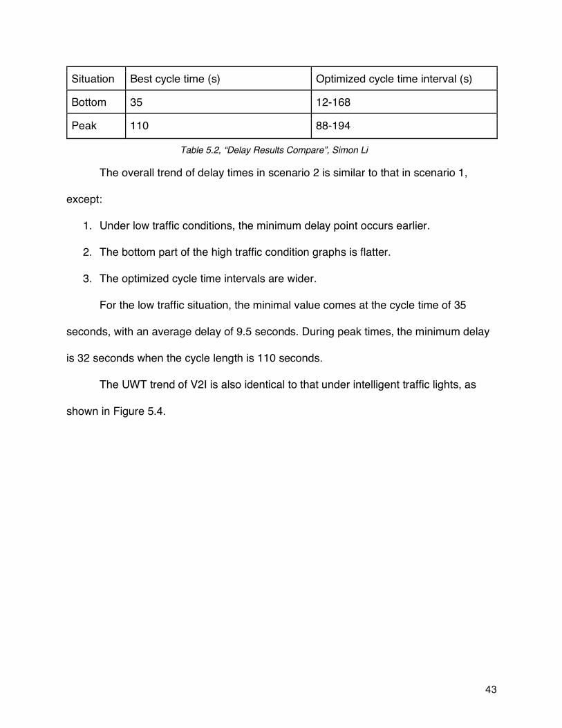
The UWT trend of V2I is also identical to that under intelligent traffic lights, as

shown in Figure 5.4.

Table 5.2, “Delay Results Compare”, Simon Li

44

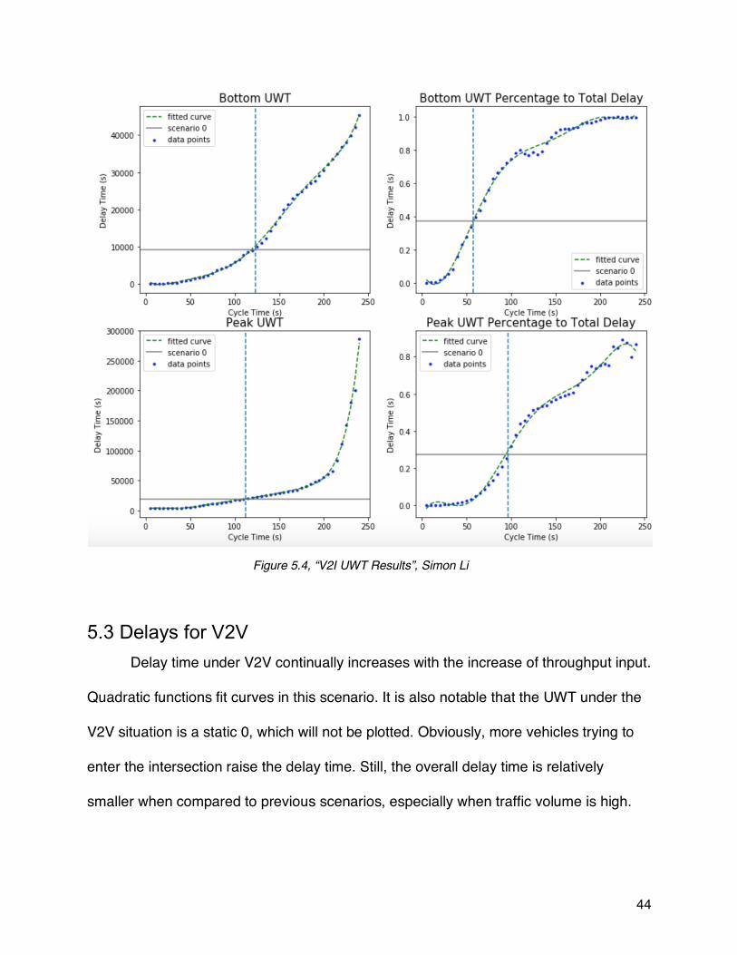
5.3 Delays for V2V Delay time under V2V continually increases with the increase of throughput input.

Quadratic functions fit curves in this scenario. It is also notable that the UWT under the

V2V situation is a static 0, which will not be plotted. Obviously, more vehicles trying to

enter the intersection raise the delay time. Still, the overall delay time is relatively

smaller when compared to previous scenarios, especially when traffic volume is high.

Figure 5.4, “V2I UWT Results”, Simon Li

45

5.4 Delay Compare

Figure 5.5, “V2V Delay Results”, Simon Li The delay time accumulated as the increase of total throughput.

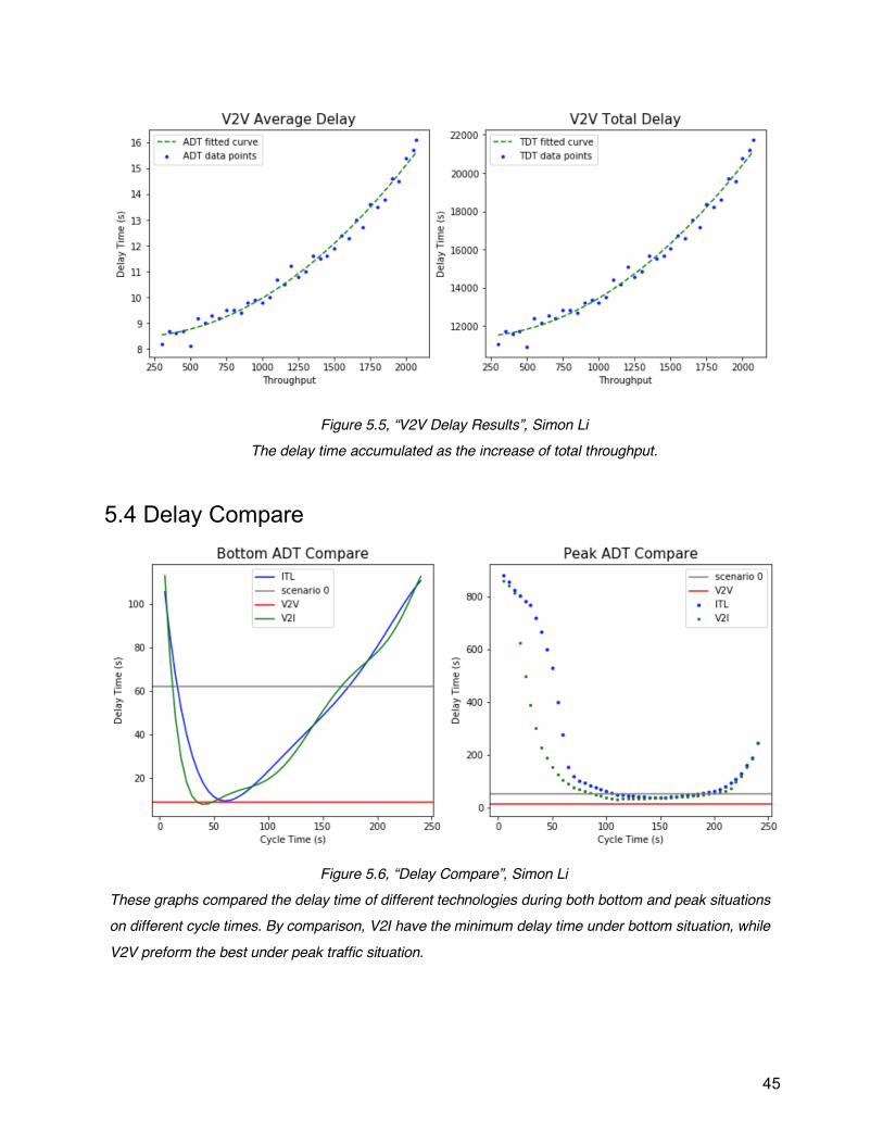
Figure 5.6, “Delay Compare”, Simon Li These graphs compared the delay time of different technologies during both bottom and peak situations on different cycle times. By comparison, V2I have the minimum delay time under bottom situation, while V2V preform the best under peak traffic situation.

46

In Figure 5.6, blue represents intelligent traffic light, green represents V2I, red

represents V2V, and grey represents the status quo. As shown, V2I performs best in

low-traffic situations, and V2V performs best under high traffic volume.

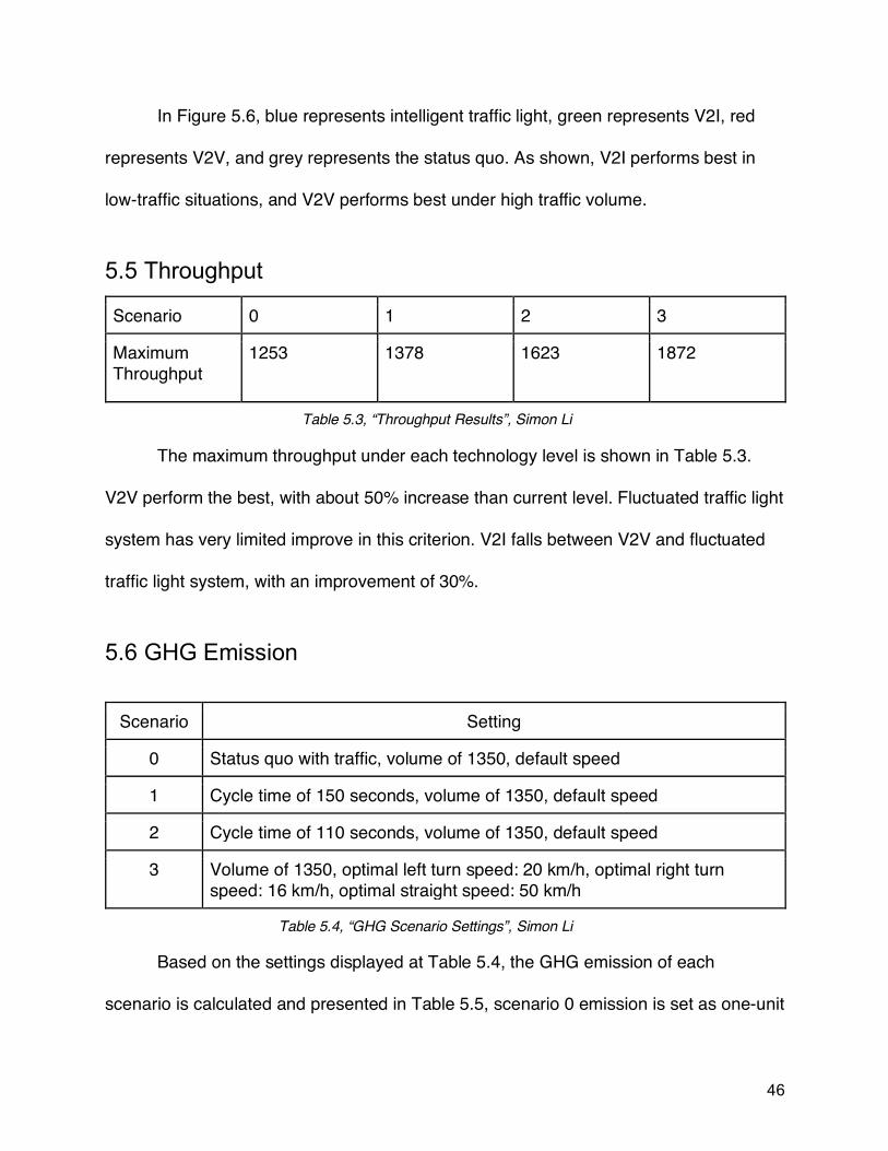
5.5 Throughput

Scenario 0 1 2 3

Maximum Throughput

1253 1378 1623 1872

The maximum throughput under each technology level is shown in Table 5.3.

V2V perform the best, with about 50% increase than current level. Fluctuated traffic light

system has very limited improve in this criterion. V2I falls between V2V and fluctuated

traffic light system, with an improvement of 30%.

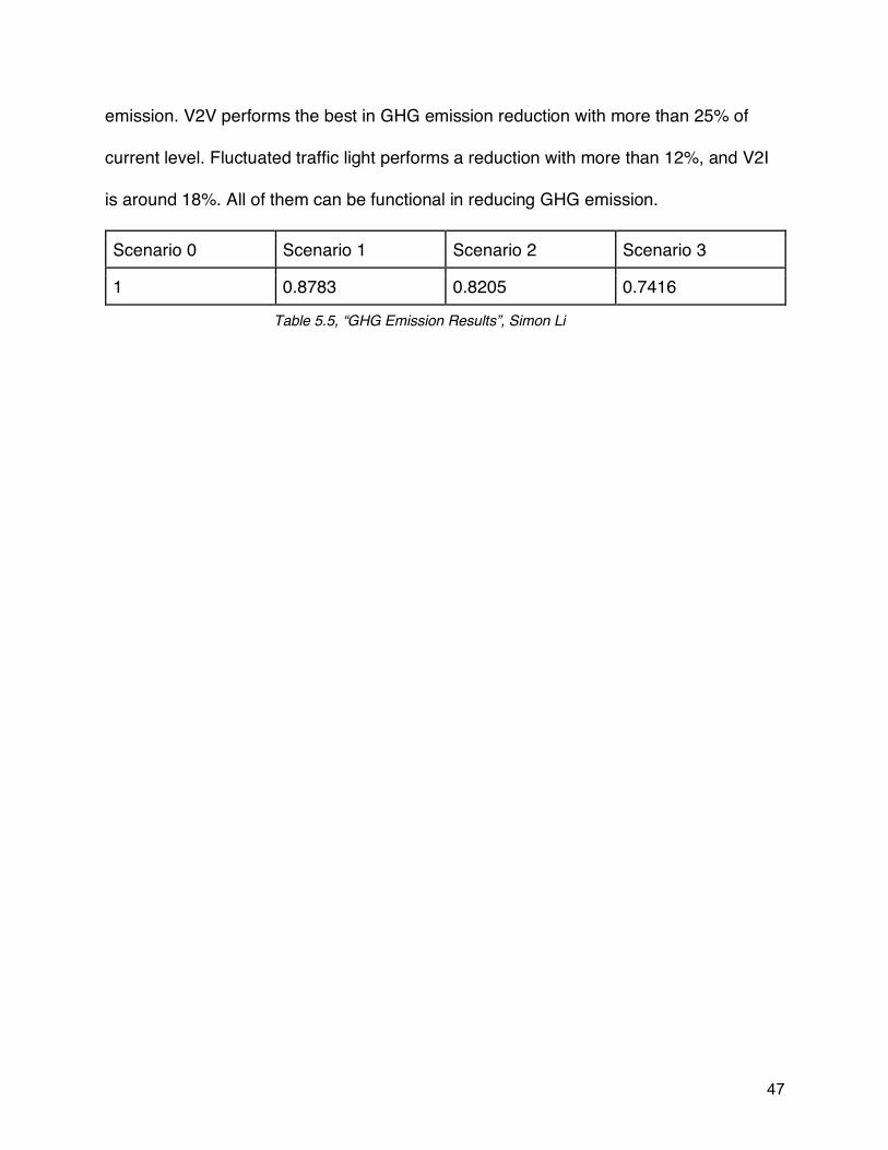
5.6 GHG Emission

Scenario Setting

0 Status quo with traffic, volume of 1350, default speed

1 Cycle time of 150 seconds, volume of 1350, default speed

2 Cycle time of 110 seconds, volume of 1350, default speed

3 Volume of 1350, optimal left turn speed: 20 km/h, optimal right turn speed: 16 km/h, optimal straight speed: 50 km/h

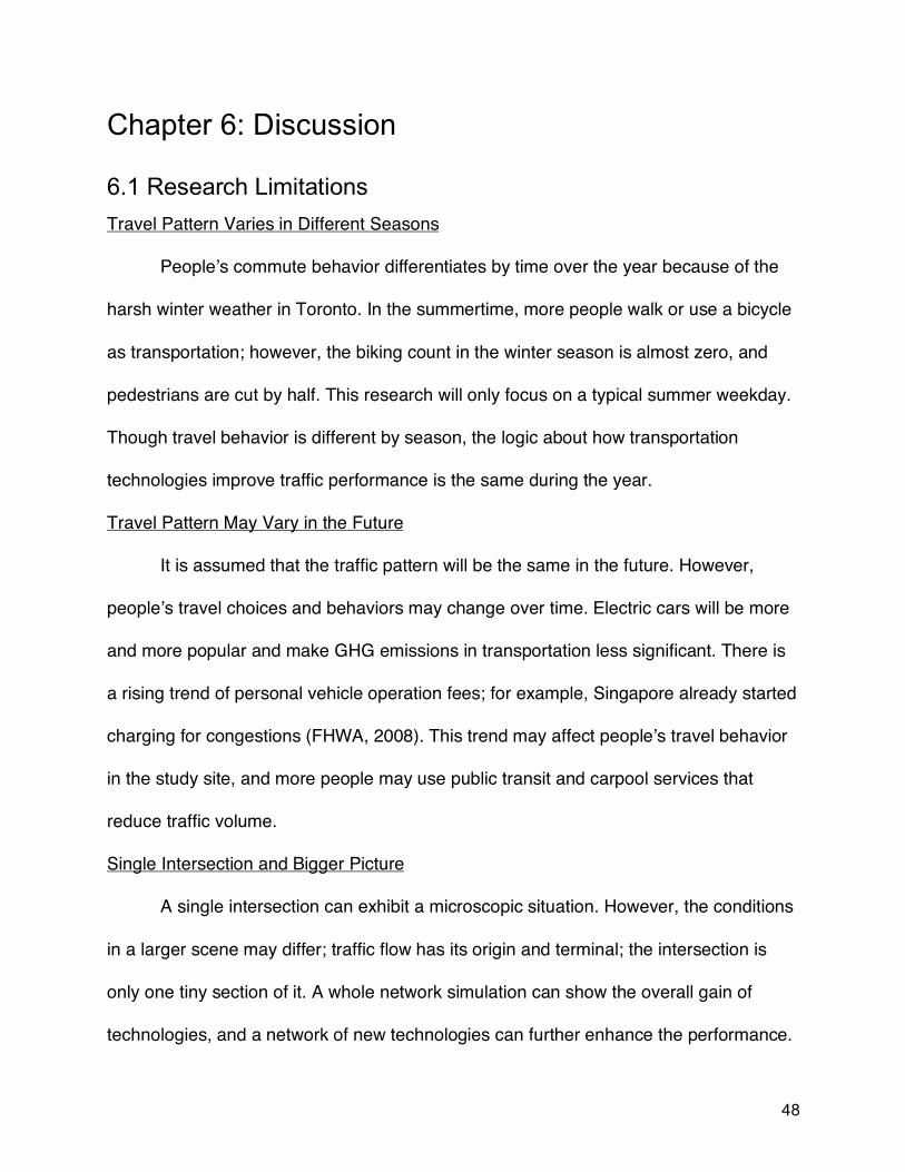
Based on the settings displayed at Table 5.4, the GHG emission of each

scenario is calculated and presented in Table 5.5, scenario 0 emission is set as one-unit

Table 5.3, “Throughput Results”, Simon Li

Table 5.4, “GHG Scenario Settings”, Simon Li

47

emission. V2V performs the best in GHG emission reduction with more than 25% of

current level. Fluctuated traffic light performs a reduction with more than 12%, and V2I

is around 18%. All of them can be functional in reducing GHG emission.

Scenario 0 Scenario 1 Scenario 2 Scenario 3

1 0.8783 0.8205 0.7416

Table 5.5, “GHG Emission Results”, Simon Li

48

Chapter 6: Discussion

6.1 Research Limitations Travel Pattern Varies in Different Seasons

People’s commute behavior differentiates by time over the year because of the

harsh winter weather in Toronto. In the summertime, more people walk or use a bicycle

as transportation; however, the biking count in the winter season is almost zero, and

pedestrians are cut by half. This research will only focus on a typical summer weekday.

Though travel behavior is different by season, the logic about how transportation

technologies improve traffic performance is the same during the year.

Travel Pattern May Vary in the Future

It is assumed that the traffic pattern will be the same in the future. However,

people’s travel choices and behaviors may change over time. Electric cars will be more

and more popular and make GHG emissions in transportation less significant. There is

a rising trend of personal vehicle operation fees; for example, Singapore already started

charging for congestions (FHWA, 2008). This trend may affect people’s travel behavior

in the study site, and more people may use public transit and carpool services that

reduce traffic volume.

Single Intersection and Bigger Picture

A single intersection can exhibit a microscopic situation. However, the conditions

in a larger scene may differ; traffic flow has its origin and terminal; the intersection is

only one tiny section of it. A whole network simulation can show the overall gain of

technologies, and a network of new technologies can further enhance the performance.

49

For example, the baseline data of this research is collected by the current traffic

situation and applied to every technology tested. However, travelers can break the

information bias by vehicular communication; they can choose a better route to

minimize their travel time, thus smooth the peak vehicle count of the study site.

6.2 Results Discussion The research results found many phenomena that are out of expectation or

display some interesting logic behind, this section will discuss some of them.

Rapid Delay Drop Under High Volume and Short Cycle Length

As shown in Figure 5.1 and 5.3, the delay time under peak traffic situation

dropped rapidly when the cycle length is short. This is mainly because when the light

turns green, the traffic cannot form a flow immediately, the vehicles need time to speed

up. Thus, when the cycle time is short, more percentage of the green time is spent at

flow formation. In other words, the correct vehicle flow time is short; thus, when the

peak volume applied, the intersection will fail to handle this significant amount of traffic

under short cycle length. As the length grows, the flow formation time will remain the

same, which means all of the time will be used for vehicle flow and drops the delay time

rapidly.

UWT of Bottom Traffic is Relatively Higher Than Peak Traffic

As the UWT results showed, UWT is relatively higher when the traffic volume is

lower. This is mainly because when the light is long, and traffic is not stacked up, more

time will be spent waiting for the red light while there is no vehicle in the intersection

conflict zone. Moreover, under higher traffic volume, the intersection conflict zone is

50

rarely empty, which means more of the waiting is because the road space they planned

to use is occupied.

V2I and V2V Delay Gap Increases as the Traffic Volume Increase

The average delay gap between V2I and V2V under the bottom traffic volume is

0.9 second, and this gap grows to 20.4 seconds, which means that V2V performs much

better when the traffic volume is high. This is mainly because the logic of V2V is to

change the vehicles’ speed to allow them to enter the intersection at the time slot they

booked for beforehand. The delay time in this research only takes the stop time into

account, and the time vehicles move at a relatively slower than usual speed will not be

considered a delay. When the traffic volume is high, more vehicles tend to stop in front

of the stop lines in the V2I scenario, but not many vehicles stop in the V2V situation,

they will adjust their speed of approach.

A Huge Leap in Throughput from Intelligent Traffic Light to V2I

As Table 5.3 displayed, the maximum throughput experienced a massive leap

from 1378 under intelligent traffic light to 1623 under V2I. The improvement comes from

the arrangement of vehicles traveling in different directions. Commonly, the left turn

vehicles fail to make the turn during the left green, wait in the middle of the road during

the whole green period that blocks one lane of traffic. However, this problem is solved

by V2I by separating the vehicle from traveling different directions by time entering the

intersection instead of lanes.

GHG is not Reduced as Much as Expected

51

Out of expectation, there is no massive reduction in greenhouse gas emissions

as the technology evolves. This indicates that travel time reduction and speed

stabilization have only minor effects of cutting emissions; the number of cars traveling is

the most important influential factor.

However, it does not mean that technologies have limited function in the

environment. This research assumes the only change between scenarios is technology.

Still, in the real-world situation, autonomous vehicles can improve car sharing, thus

cutting the number of rides, and the technology improvement will not only effect on-road

technologies but also things inside the vehicles, more electric vehicles with zero-

emission will help to save the environment.

6.3 Challenges and Opportunities to Urban Planners The first challenge planners may face is should cities embrace the new

transportation technologies. The traffic volume and time delay are just like the price and

quantity in the economy demand and supply chart. If new technologies come true, delay

time is reduced, the trip demand will actually increase until a new equilibrium is

reached. Though in the new equilibrium, delay time will be lower, but introducing more

vehicles into the city is kind of in conflict with planning priorities of major cities over the

world nowadays, which is like building a walkable city or people’s city instead of a city of

cars. This makes many planners and designers hesitate or even refuse new

transportation technologies. However, many other planners believe that more people

use cars because their needs are not fulfilled, and fulfilling the needs of residents ranks

even higher than building a walkable city in planning priorities. There are still debates

52

going on, I personally believe although the process is painful, the outcomes might not

be that pessimistic. Delay reduction can improve residents’ living quality. And more

vehicles not equal to more personal vehicles, car sharing are also believed to be more

popular during the autonomous vehicle age.

As for the possible increase of car-sharing business, some scholars pointed out

that there will be new infrastructures and networks in favor of autonomous car-sharing

or van-sharing, and the passenger share of buses and subways may drop. How our

transportation planners prepare all of this is also challenging. It is possible that in the

future, the subway trains will be replaced by more flexible autonomous cars, and the

tunnels are turned into underground autonomous taxi stations. It is also possible that

the buses are replaced by van-sharing. Actually, Via already did some of this works in

some small cities and the outcome are very positive.

Car-sharing can also decrease the need for parking lots in the city. Currently,

many city core lands are used as public parking lots, trains parking lots, and buses

parking lots. Car-sharing can decrease the needs of parking dramatically, thus release a

huge amount of valuable lands. Planners should be prepared and take advantage of

these possible land use changes.

53

References Amin-Naseri, M., Chakraborty, P., Sharma, A., Gilbert, S. B., & Hong, M. (2018).

Evaluating the Reliability, Coverage, and Added Value of Crowdsourced Traffic

Incident Reports from Waze. Transportation Research Record: Journal of the

Transportation Research Board, 2672(43), 34–43.

https://doi.org/10.1177/0361198118790619

Amirgholy, M., Nourinejad, M., & Gao, H. O. (2019). Optimal traffic control at smart

intersections: Automated network fundamental diagram. Transportation

Research Part B: Methodological, S0191261519302449.

https://doi.org/10.1016/j.trb.2019.10.001

Anisimov, I., Burakova, A., Burakova, O., & Burakova, L. (2018). Evaluation of the traffic

signal regulation efficiency of crossroads with unstable transport demand by

time. MATEC Web of Conferences, 170, 05013.

https://doi.org/10.1051/matecconf/201817005013

Atallah, R., Khabbaz, M., & Assi, C. (2017). Multihop V2I Communications: A Feasibility

Study, Modeling, and Performance Analysis. IEEE Transactions on Vehicular

Technology, 66(3), 2801–2810. https://doi.org/10.1109/TVT.2016.2586758

Bani Younes, M., & Boukerche, A. (2015). A performance evaluation of an efficient

traffic congestion detection protocol (ECODE) for intelligent transportation

systems. Ad Hoc Networks, 24, 317–336.

https://doi.org/10.1016/j.adhoc.2014.09.005

54

Bazzan, A. L. C., & Klügl, F. (2014). A review on agent-based technology for traffic and

transportation. The Knowledge Engineering Review, 29(3), 375–403.

https://doi.org/10.1017/S0269888913000118

Bifulco, G., Galante, F., Pariota, L., & Spena, M. (2015). A Linear Model for the

Estimation of Fuel Consumption and the Impact Evaluation of Advanced Driving

Assistance Systems. Sustainability, 7(10), 14326–14343.

https://doi.org/10.3390/su71014326

Bo, Z., Di, W., MinYi, Z., Nong, Z., & Lin, H. (2019). Electric vehicle energy predictive

optimal control by V2I communication. Advances in Mechanical Engineering,

11(2), 168781401882152. https://doi.org/10.1177/1687814018821523

Buck, H. S., Mallig, N., & Vortisch, P. (2017). Calibrating Vissim to Analyze Delay at

Signalized Intersections. Transportation Research Record: Journal of the

Transportation Research Board, 2615(1), 73–81. https://doi.org/10.3141/2615-09

Butakov, V. A., & Ioannou, P. (2016). Personalized Driver Assistance for Signalized

Intersections Using V2I Communication. IEEE Transactions on Intelligent

Transportation Systems, 17(7), 1910–1919.

https://doi.org/10.1109/TITS.2016.2515023

Cheevarunothai, P., & Kaewpikul, R. (2019). Empirical Study on Maximum Traffic

Throughputs at Intersections. MATEC Web of Conferences, 259, 02008.


55

Chodur, J., & Ostrowski, K. (2019). Speed models and criteria for assessing traffic

performance on two-lane highways. MATEC Web of Conferences, 262, 05004.


Courmont, A. (2018). Plateforme, big data et recomposition du gouvernement urbain:

Les effets de Waze sur les politiques de régulation du trafic. Revue française de

sociologie, 59(3), 423. https://doi.org/10.3917/rfs.593.0423

Dey, K. C., Rayamajhi, A., Chowdhury, M., Bhavsar, P., & Martin, J. (2016a). Vehicle-

to-vehicle (V2V) and vehicle-to-infrastructure (V2I) communication in a

heterogeneous wireless network – Performance evaluation. Transportation

Research Part C: Emerging Technologies, 68, 168–184.

https://doi.org/10.1016/j.trc.2016.03.008

Dey, K. C., Rayamajhi, A., Chowdhury, M., Bhavsar, P., & Martin, J. (2016b). Vehicle-

to-vehicle (V2V) and vehicle-to-infrastructure (V2I) communication in a

heterogeneous wireless network – Performance evaluation. Transportation

Research Part C: Emerging Technologies, 68, 168–184.


Fitzgerald, E., & Landfeldt, B. (2015). Increasing Road Traffic Throughput through

Dynamic Traffic Accident Risk Mitigation. Journal of Transportation

Technologies, 05(04), 223–239. https://doi.org/10.4236/jtts.2015.54021

Giridhar, A., & Kumar, P. R. (2006). Scheduling Automated Traffic on a Network of

Roads. IEEE Transactions on Vehicular Technology, 55(5), 1467–1474.

https://doi.org/10.1109/TVT.2006.877472

56

Gomes, G., May, A., & Horowitz, R. (2004). Congested Freeway Microsimulation Model

Using VISSIM. Transportation Research Record: Journal of the Transportation

Research Board, 1876(1), 71–81. https://doi.org/10.3141/1876-08

Gupta, S., Vasardani, M., & Winter, S. (2019a). Negotiation Between Vehicles and

Pedestrians for the Right of Way at Intersections. IEEE Transactions on

Intelligent Transportation Systems, 20(3), 888–899.


Gupta, S., Vasardani, M., & Winter, S. (2019b). Negotiation Between Vehicles and

Pedestrians for the Right of Way at Intersections. IEEE Transactions on



Han, M.-J., Lin, C.-H., & Song, K.-T. (2013). Robotic Emotional Expression Generation

Based on Mood Transition and Personality Model. IEEE Transactions on

Cybernetics, 43(4), 1290–1303. https://doi.org/10.1109/TSMCB.2012.2228851

Hashimoto, Y., Gu, Y., Hsu, L.-T., Iryo-Asano, M., & Kamijo, S. (2016). A probabilistic

model of pedestrian crossing behavior at signalized intersections for connected

vehicles. Transportation Research Part C: Emerging Technologies, 71, 164–181.


Hatami, H., & Aghayan, I. (2017). Traffic Efficiency Evaluation of Elliptical Roundabout

Compared with Modern and Turbo Roundabouts Considering Traffic Signal

Control. PROMET - Traffic&Transportation, 29(1), 1–11.

https://doi.org/10.7307/ptt.v29i1.2053

57

He, S., Li, J., & Qiu, T. Z. (2017). Vehicle-to-Pedestrian Communication Modeling and

Collision Avoiding Method in Connected Vehicle Environment. Transportation

Research Record: Journal of the Transportation Research Board, 2621(1), 21–

30. https://doi.org/10.3141/2621-03

Helbing, D. (2009). Derivation of a fundamental diagram for urban traffic flow. The

European Physical Journal B, 70(2), 229–241.

https://doi.org/10.1140/epjb/e2009-00093-7

Jabali, O., Van Woensel, T., & de Kok, A. G. (2012). Analysis of Travel Times and CO 2

Emissions in Time-Dependent Vehicle Routing. Production and Operations

Management, 21(6), 1060–1074. https://doi.org/10.1111/j.1937-

5956.2012.01338.x

Jia, D., & Ngoduy, D. (2016). Enhanced cooperative car-following traffic model with the

combination of V2V and V2I communication. Transportation Research Part B:

Methodological, 90, 172–191. https://doi.org/10.1016/j.trb.2016.03.008

Jung, S., Lee, M., Kim, J., Lyu, Y., & Park, J. (2011). Speed‐dependent emission of air

pollutants from gasoline‐powered passenger cars. Environmental Technology,

32(11), 1173–1181. https://doi.org/10.1080/09593330.2010.505611

Kalatian, A., & Farooq, B. (2019). DeepWait: Pedestrian Wait Time Estimation in Mixed

Traffic Conditions Using Deep Survival Analysis. ArXiv:1904.11008 [Cs].

http://arxiv.org/abs/1904.11008

58

Kellner, F. (2016). Exploring the impact of traffic congestion on CO2 emissions in freight

distribution networks. Logistics Research, 9(1), 21.

https://doi.org/10.1007/s12159-016-0148-5

Kerimov, M., Safiullin, R., Marusin, A., & Marusin, A. (2017). Evaluation of Functional

Efficiency of Automated Traffic Enforcement Systems. Transportation Research

Procedia, 20, 288–294. https://doi.org/10.1016/j.trpro.2017.01.025

Khader, A. I., & Martin, R. S. (2019). On-the-road testing of the effects of driver’s

experience, gender, speed, and road grade on car emissions. Journal of the Air

& Waste Management Association, 69(10), 1182–1194.

https://doi.org/10.1080/10962247.2019.1640804

Kowshik, H., Caveney, D., & Kumar, P. R. (2011). Provable Systemwide Safety in

Intelligent Intersections. IEEE Transactions on Vehicular Technology, 60(3),

804–818. https://doi.org/10.1109/TVT.2011.2107584

Krajzewicz, D., Hertkorn, G., Wagner, P., & Rössel, C. (n.d.). SUMO (Simulation of

Urban MObility). 5.

Lämmer, S., & Helbing, D. (2008a). Self-control of traffic lights and vehicle flows in

urban road networks. Journal of Statistical Mechanics: Theory and Experiment,

2008(04), P04019. https://doi.org/10.1088/1742-5468/2008/04/P04019

Lämmer, S., & Helbing, D. (2008b). Self-control of traffic lights and vehicle flows in

urban road networks. Journal of Statistical Mechanics: Theory and Experiment,

2008(04), P04019. https://doi.org/10.1088/1742-5468/2008/04/P04019

59

Lee, J., & Park, B. (2012). Development and Evaluation of a Cooperative Vehicle

Intersection Control Algorithm Under the Connected Vehicles Environment. IEEE

Transactions on Intelligent Transportation Systems, 13(1), 81–90.


Li, Zhixia, Chitturi, M. V., Zheng, D., Bill, A. R., & Noyce, D. A. (2013). Modeling

Reservation-Based Autonomous Intersection Control in VISSIM. Transportation

Research Record: Journal of the Transportation Research Board, 2381(1), 81–

90. https://doi.org/10.3141/2381-10

Li, Zhuofei, & Elefteriadou, L. (2013). Maximizing the Traffic Throughput of Turn Bays at

a Signalized Intersection Approach. Journal of Transportation Engineering,

139(5), 425–432. https://doi.org/10.1061/(ASCE)TE.1943-5436.0000514

Liberman, M. (2019). Commentary: “Proceed to and follow the highlighted route”—

Thoracic surgical Waze is here. The Journal of Thoracic and Cardiovascular

Surgery, 157(5), 2036–2037. https://doi.org/10.1016/j.jtcvs.2019.01.005

Liu, C., Susilo, Y. O., & Karlström, A. (2015). The influence of weather characteristics

variability on individual’s travel mode choice in different seasons and regions in

Sweden. Transport Policy, 41, 147–158.

https://doi.org/10.1016/j.tranpol.2015.01.001

Lu, Z., Fu, T., Fu, L., Shiravi, S., & Jiang, C. (2016). A video-based approach to

calibrating car-following parameters in VISSIM for urban traffic. International

Journal of Transportation Science and Technology, 5(1), 1–9.

https://doi.org/10.1016/j.ijtst.2016.06.001

60

Milanes, V., Villagra, J., Godoy, J., Simo, J., Perez, J., & Onieva, E. (2012). An

Intelligent V2I-Based Traffic Management System. IEEE Transactions on



Millard-Ball, A. (2018a). Pedestrians, Autonomous Vehicles, and Cities. Journal of

Planning Education and Research, 38(1), 6–12.

https://doi.org/10.1177/0739456X16675674

Millard-Ball, A. (2018b). Pedestrians, Autonomous Vehicles, and Cities. Journal of

Planning Education and Research, 38(1), 6–12.

https://doi.org/10.1177/0739456X16675674

Mumtaz, S., Saidul Huq, K. M., Ashraf, M. I., Rodriguez, J., Monteiro, V., & Politis, C.

(2015). Cognitive vehicular communication for 5G. IEEE Communications

Magazine, 53(7), 109–117. https://doi.org/10.1109/MCOM.2015.7158273

Papadimitratos, P., La Fortelle, A., Evenssen, K., Brignolo, R., & Cosenza, S. (2009).

Vehicular communication systems: Enabling technologies, applications, and

future outlook on intelligent transportation. IEEE Communications Magazine,

47(11), 84–95. https://doi.org/10.1109/MCOM.2009.5307471

Papageorgiou, M. (Ed.). (1991). Concise encyclopedia of traffic & transportation

systems (1st ed). Pergamon Press.

Papageorgiou, M., Kiakaki, C., Dinopoulou, V., Kotsialos, A., & Yibing Wang. (2003).

Review of road traffic control strategies. Proceedings of the IEEE, 91(12), 2043–

2067. https://doi.org/10.1109/JPROC.2003.819610

61

Qian, X., Altché, F., Grégoire, J., & de La Fortelle, A. (2017). Autonomous Intersection

Management systems: Criteria, implementation and evaluation. IET Intelligent

Transport Systems, 11(3), 182–189. https://doi.org/10.1049/iet-its.2016.0043

Schebesch, R., Toop, E., Sturges, D., & Fast, V. (2017). The Impact of Connected and

Automated Vehicles on Pedestrians ( symposia ). Journal of Transport & Health,

7, S71–S72. https://doi.org/10.1016/j.jth.2017.11.116

Shah, S. A. A., Ahmed, E., Imran, M., & Zeadally, S. (2018). 5G for Vehicular

Communications. IEEE Communications Magazine, 56(1), 111–117.

https://doi.org/10.1109/MCOM.2018.1700467

Silva, C. M., Aquino, A. L. L., & Meira, W. (2015). Smart Traffic Light for Low Traffic

Conditions: A Solution for Improving the Drivers Safety. Mobile Networks and

Applications, 20(2), 285–293. https://doi.org/10.1007/s11036-015-0571-x

Song, G., Yu, L., & Zhang, Y. (2012). Applicability of Traffic Microsimulation Models in

Vehicle Emissions Estimates: Case Study of VISSIM. Transportation Research

Record: Journal of the Transportation Research Board, 2270(1), 132–141.

https://doi.org/10.3141/2270-16

Spitzer-Shohat, S., & Chin, M. H. (2019). The “Waze” of Inequity Reduction

Frameworks for Organizations: A Scoping Review. Journal of General Internal

Medicine, 34(4), 604–617. https://doi.org/10.1007/s11606-019-04829-7

Starzyk, J. A., Graham, J., & Puzio, L. (2017). Needs, Pains, and Motivations in

Autonomous Agents. IEEE Transactions on Neural Networks and Learning

Systems, 28(11), 2528–2540. https://doi.org/10.1109/TNNLS.2016.2596787

62

Stevanovic, A., Stevanovic, J., Zhang, K., & Batterman, S. (2009). Optimizing Traffic

Control to Reduce Fuel Consumption and Vehicular Emissions: Integrated

Approach with VISSIM, CMEM, and VISGAOST. Transportation Research

Record: Journal of the Transportation Research Board, 2128(1), 105–113.

https://doi.org/10.3141/2128-11

Tachet, R., Santi, P., Sobolevsky, S., Reyes-Castro, L. I., Frazzoli, E., Helbing, D., &

Ratti, C. (2016a). Revisiting Street Intersections Using Slot-Based Systems.

PLOS ONE, 11(3), e0149607. https://doi.org/10.1371/journal.pone.0149607

Tachet, R., Santi, P., Sobolevsky, S., Reyes-Castro, L. I., Frazzoli, E., Helbing, D., &

Ratti, C. (2016b). Revisiting Street Intersections Using Slot-Based Systems.

PLOS ONE, 11(3), e0149607. https://doi.org/10.1371/journal.pone.0149607

Talebpour, A., & Mahmassani, H. S. (2016). Influence of connected and autonomous

vehicles on traffic flow stability and throughput. Transportation Research Part C:

Emerging Technologies, 71, 143–163. https://doi.org/10.1016/j.trc.2016.07.007

Tang, T.-Q., Huang, H.-J., & Shang, H.-Y. (2010). A DYNAMIC MODEL FOR THE

HETEROGENEOUS TRAFFIC FLOW CONSISTING OF CAR, BICYCLE AND

PEDESTRIAN. International Journal of Modern Physics C, 21(02), 159–176.

https://doi.org/10.1142/S0129183110015038

Truong, T. T. P. (n.d.). Equilibria in the multi-criteria traffic networks. 125.

Uzcategui, R. A., De Sucre, A. J., & Acosta-Marum, G. (2009). Wave: A tutorial. IEEE

Communications Magazine, 47(5), 126–133.

https://doi.org/10.1109/MCOM.2009.4939288

63

Van der Graaf, S. (2018). In Waze We Trust: Algorithmic Governance of the Public

Sphere. Media and Communication, 6(4), 153.

https://doi.org/10.17645/mac.v6i4.1710

Van Hecke, T. (2008). Minimizing the delay at traffic lights. Teaching Mathematics and

Its Applications, 28(1), 38–42. https://doi.org/10.1093/teamat/hrp002

van Leeuwaarden, J. S. H. (2006). Delay Analysis for the Fixed-Cycle Traffic-Light

Queue. Transportation Science, 40(2), 189–199.

https://doi.org/10.1287/trsc.1050.0125

Wang, J., Iwasaki, R., Bayen, A. M., & Harvey, J. (2016). Future road transportation

technology. International Journal of Transportation Science and Technology,

5(1), iii–iv. https://doi.org/10.1016/j.ijtst.2016.09.001

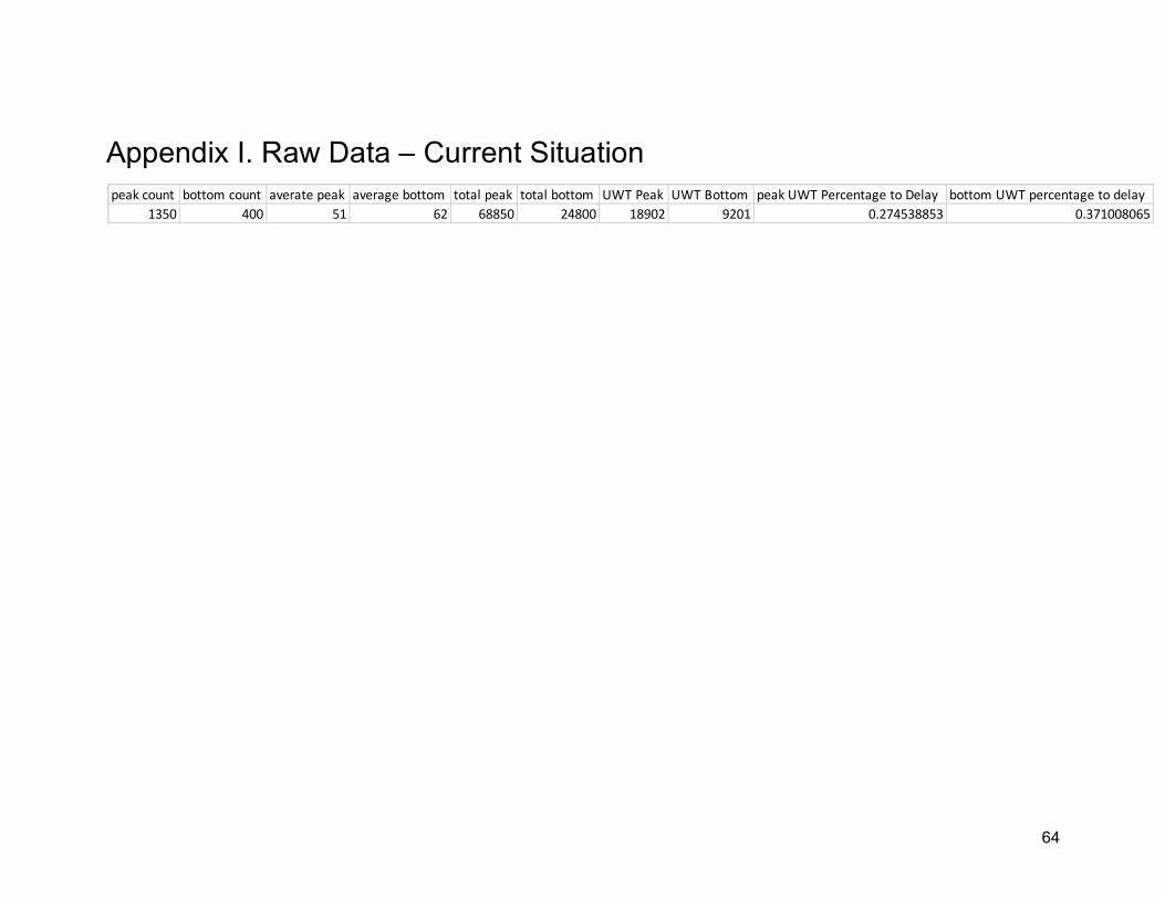
64

Appendix I. Raw Data – Current Situation

peak count bottom count averate peak average bottom total peak total bottom UWT Peak UWT Bottom peak UWT Percentage to Delay bottom UWT percentage to delay1350 400 51 62 68850 24800 18902 9201 0.274538853 0.371008065

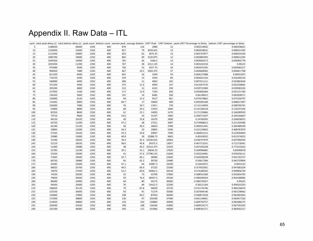
65

Appendix II. Raw Data – ITL

cycle total peak delay (s) total bottom delay (s) peak count bottom count averate peak average bottom UWT Peak UWT Bottom peak UWT Percentage to Delay bottom UWT percentage to delay5 1186650 46400 1350 400 879 116 2984 12 0.002514642 0.000258621

10 1156950 31600 1350 400 857 79 3029.625 13 0.002618631 0.00041139215 1111050 24800 1350 400 823 62 3075.25 13 0.002767877 0.00052419420 1082700 19600 1350 400 802 49 3120.875 12 0.002882493 0.00061224525 1054350 14400 1350 400 781 36 3166.5 13 0.003003272 0.00090277830 1035450 11200 1350 400 767 28 3212.125 14 0.003102154 0.0012535 972000 9200 1350 400 720 23 3257.75 19 0.003351595 0.00206521740 900450 7680 1350 400 667 19.2 3303.375 37 0.003668582 0.00481770845 811350 6400 1350 400 601 16 3349 59 0.004127688 0.0092187550 714150 5200 1350 400 529 13 3593 85 0.005031156 0.01634615455 540000 4400 1350 400 400 11 4002 105 0.007411111 0.02386363660 371250 4560 1350 400 275 11.4 4959 147 0.013357576 0.03223684265 205200 4800 1350 400 152 12 6101 190 0.029731969 0.03958333370 157950 5160 1350 400 117 12.9 7243 269 0.045856284 0.05213178375 136350 5600 1350 400 101 14 8385 358 0.06149615 0.06392857180 126900 6120 1350 400 94 15.3 9527 461 0.075074862 0.07532679785 114345 6800 1350 400 84.7 17 10669 589 0.093305348 0.08661764790 102600 7480 1350 400 76 18.7 11811 739 0.115116959 0.09879679195 91800 8080 1350 400 68 20.2 12953 1004 0.141100218 0.124257426

100 82350 8840 1350 400 61 22.1 14095 1470 0.171159684 0.166289593105 73710 9600 1350 400 54.6 24 15237 1960 0.206715507 0.204166667110 66150 10320 1350 400 49 25.8 16379 2690 0.24760393 0.260658915115 63720 11200 1350 400 47.2 28 17521 3487 0.274968613 0.311339286120 62100 12120 1350 400 46 30.3 18663 4780 0.300531401 0.394389439125 59805 13200 1350 400 44.3 33 19805 5396 0.331159602 0.408787879130 57105 14320 1350 400 42.3 35.8 20947 7490 0.366815515 0.523044693135 55080 15600 1350 400 40.8 39 22088.75 9603 0.40103032 0.615576923140 53190 16920 1350 400 39.4 42.3 23230.625 10964 0.436747979 0.647990544145 52110 18320 1350 400 38.6 45.8 24372.5 13057 0.467712531 0.712718341150 51300 19680 1350 400 38 49.2 25514.375 15203 0.497356238 0.772510163155 52785 21240 1350 400 39.1 53.1 26656.25 17829 0.504996685 0.83940678160 55350 23040 1350 400 41 57.6 27798.125 21640 0.502224481 0.939236111165 57645 24040 1350 400 42.7 60.1 28940 22640 0.502038338 0.941763727170 60750 24880 1350 400 45 62.2 30750 23480 0.50617284 0.943729904175 63585 25600 1350 400 47.1 64 33987.5 24200 0.53452072 0.9453125180 66825 26760 1350 400 49.5 66.9 37225 25360 0.557052001 0.947683109185 70470 27920 1350 400 52.2 69.8 40462.5 26520 0.574180502 0.949856734190 74250 29200 1350 400 55 73 43700 27800 0.588552189 0.952054795195 79650 30560 1350 400 59 76.4 46937.5 29160 0.589296924 0.954188482200 86400 32000 1350 400 64 80 50175 30600 0.580729167 0.95625205 94500 33600 1350 400 70 84 53412.5 32200 0.56521164 0.958333333210 106650 35120 1350 400 79 87.8 56650 33720 0.531176746 0.960136674215 125550 36400 1350 400 93 91 71274 35000 0.567694146 0.961538462220 145800 37800 1350 400 108 94.5 87024 36400 0.596872428 0.962962963225 175500 38800 1350 400 130 97 105500 37400 0.601139601 0.963917526230 214650 40800 1350 400 159 102 130883 39400 0.609750757 0.965686275235 256500 43200 1350 400 190 108 156266 41800 0.609224172 0.967592593240 332100 46000 1350 400 246 115 231866 44600 0.698181271 0.969565217

66

Appendix III. Raw Data – V2I

cycle peak count bottom count averate peak average bottom total peak total bottom UWT Peak UWT Bottom peak UWT Percentage to Delay bottom UWT percentage to delay5 1350 400 858 112 1158300 44800 3274 102 0.002826556 0.002276786

10 1350 400 840 75 1134000 30000 3285 135 0.002896825 0.004515 1350 400 814 52 1098900 20800 3309 158 0.003011193 0.00759615420 1350 400 624 23 842400 9200 3342 186 0.003967236 0.02021739125 1350 400 497 15 670950 6000 3372 214 0.00502571 0.03566666730 1350 400 389 11.7 525150 4680 3491 256 0.006647624 0.05470085535 1350 400 302 9.5 407700 3800 3547 312 0.008700025 0.08210526340 1350 400 228 9.9 307800 3960 3750 632 0.012183236 0.1595959645 1350 400 187 10.2 252450 4080 4694 953 0.018593781 0.23357843150 1350 400 152 10.5 205200 4200 5304 1176 0.025847953 0.2855 1350 400 124 10.8 167400 4320 6002 1462 0.035854241 0.33842592660 1350 400 103 11.2 139050 4480 6959 1783 0.050046746 0.39799107165 1350 400 89 11.6 120150 4640 8101 2020 0.067424053 0.43534482870 1350 400 77 12 103950 4800 9243 2376 0.088917749 0.49575 1350 400 69 13.4 93150 5360 10385 3009 0.111486849 0.56138059780 1350 400 62 14.7 83700 5880 11527 3682 0.137718041 0.62619047685 1350 400 55.3 15.8 74655 6320 12669 4201 0.169700623 0.6647151990 1350 400 49.2 16.7 66420 6680 13811 4627 0.207934357 0.69266467195 1350 400 44 18 59400 7200 14953 5198 0.251734007 0.721944444

100 1350 400 39.2 19.8 52920 7920 16835 5902 0.318121693 0.74520202105 1350 400 35 21.4 47250 8560 17908 6673 0.379005291 0.779556075110 1350 400 32 24.3 43200 9720 18942 7758 0.438472222 0.798148148115 1350 400 32.5 27.5 43875 11000 20017 8566 0.45622792 0.778727273120 1350 400 32.7 29.3 44145 11720 21470 9023 0.486351795 0.769880546125 1350 400 33 31.6 44550 12640 22809 9950 0.511986532 0.787183544130 1350 400 33.8 35.6 45630 14240 23805 11023 0.521696252 0.774087079135 1350 400 34.7 39 46845 15600 25088.75 12352.5 0.535569431 0.791826923140 1350 400 36 42.4 48600 16960 26230.625 14245.625 0.539724794 0.839954304145 1350 400 36.2 46 48870 18400 27372.5 16138.75 0.560108451 0.877105978150 1350 400 37 50 49950 20000 28514.375 18031.875 0.570858358 0.90159375155 1350 400 37.6 54 50760 21600 29656.25 19925 0.584244484 0.922453704160 1350 400 38.5 57.9 51975 23160 30798.125 21420 0.592556518 0.924870466165 1350 400 39.6 62.1 53460 24840 31940 23067 0.597456042 0.928623188170 1350 400 41.2 64.5 55620 25800 33750 24003 0.606796117 0.930348837175 1350 400 42.4 66.7 57240 26680 36987.5 24960 0.646182739 0.935532234180 1350 400 44 68 59400 27200 40225 26109 0.677188552 0.959889706185 1350 400 45.7 70 61695 28000 44293 26998 0.717935003 0.964214286190 1350 400 47 72.2 63450 28880 47462 27800 0.748022065 0.962603878195 1350 400 50.2 75 67770 30000 50002 29160 0.737819094 0.972200 1350 400 54 78 72900 31200 55023 30600 0.754773663 0.980769231205 1350 400 58.4 81.2 78840 32480 60002 32200 0.761060375 0.99137931210 1350 400 64 84.6 86400 33840 65027 33602 0.752627315 0.992966903215 1350 400 72 88 97200 35200 83046 35000 0.854382716 0.994318182220 1350 400 97 92.3 130950 36920 110586 36840 0.844490263 0.997833153225 1350 400 119 95.7 160650 38280 142934 37997 0.889723 0.992607106230 1350 400 152 100.2 205200 40080 179840 39976 0.876413255 0.99740519235 1350 400 186 106 251100 42400 200329 42192 0.797805655 0.99509434240 1350 400 245 114 330750 45600 286403 45397 0.865919879 0.995548246

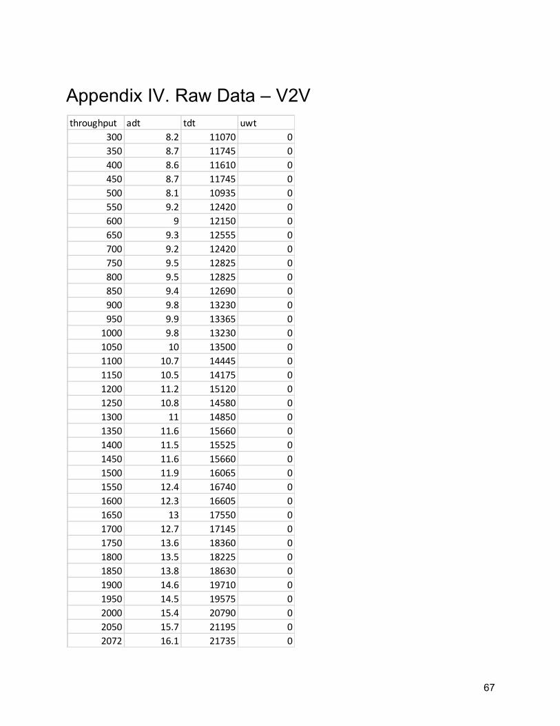
67

Appendix IV. Raw Data – V2V

throughput adt tdt uwt300 8.2 11070 0350 8.7 11745 0400 8.6 11610 0450 8.7 11745 0500 8.1 10935 0550 9.2 12420 0600 9 12150 0650 9.3 12555 0700 9.2 12420 0750 9.5 12825 0800 9.5 12825 0850 9.4 12690 0900 9.8 13230 0950 9.9 13365 01000 9.8 13230 01050 10 13500 01100 10.7 14445 01150 10.5 14175 01200 11.2 15120 01250 10.8 14580 01300 11 14850 01350 11.6 15660 01400 11.5 15525 01450 11.6 15660 01500 11.9 16065 01550 12.4 16740 01600 12.3 16605 01650 13 17550 01700 12.7 17145 01750 13.6 18360 01800 13.5 18225 01850 13.8 18630 01900 14.6 19710 01950 14.5 19575 02000 15.4 20790 02050 15.7 21195 02072 16.1 21735 0

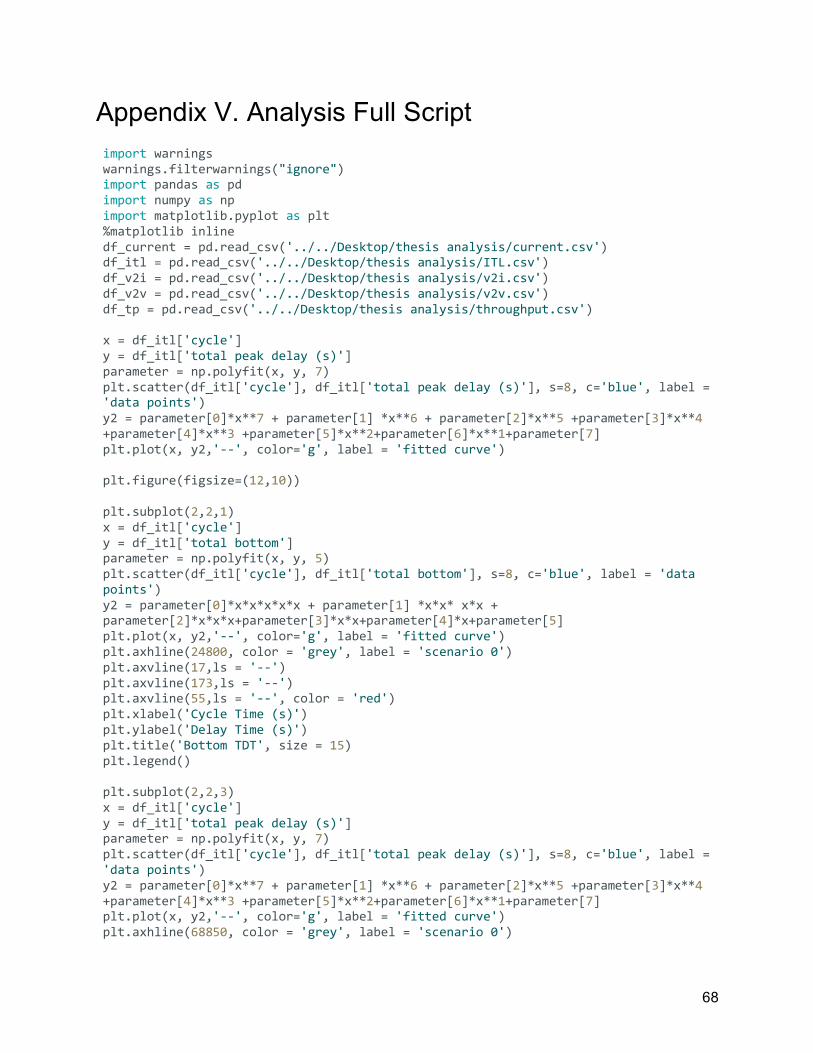
68

Appendix V. Analysis Full Script import warnings warnings.filterwarnings("ignore") import pandas as pd import numpy as np import matplotlib.pyplot as plt %matplotlib inline df_current = pd.read_csv('../../Desktop/thesis analysis/current.csv') df_itl = pd.read_csv('../../Desktop/thesis analysis/ITL.csv') df_v2i = pd.read_csv('../../Desktop/thesis analysis/v2i.csv') df_v2v = pd.read_csv('../../Desktop/thesis analysis/v2v.csv') df_tp = pd.read_csv('../../Desktop/thesis analysis/throughput.csv') x = df_itl['cycle'] y = df_itl['total peak delay (s)'] parameter = np.polyfit(x, y, 7) plt.scatter(df_itl['cycle'], df_itl['total peak delay (s)'], s=8, c='blue', label = 'data points') y2 = parameter[0]*x**7 + parameter[1] *x**6 + parameter[2]*x**5 +parameter[3]*x**4 +parameter[4]*x**3 +parameter[5]*x**2+parameter[6]*x**1+parameter[7] plt.plot(x, y2,'--', color='g', label = 'fitted curve') plt.figure(figsize=(12,10)) plt.subplot(2,2,1) x = df_itl['cycle'] y = df_itl['total bottom'] parameter = np.polyfit(x, y, 5) plt.scatter(df_itl['cycle'], df_itl['total bottom'], s=8, c='blue', label = 'data points') y2 = parameter[0]*x*x*x*x*x + parameter[1] *x*x* x*x + parameter[2]*x*x*x+parameter[3]*x*x+parameter[4]*x+parameter[5] plt.plot(x, y2,'--', color='g', label = 'fitted curve') plt.axhline(24800, color = 'grey', label = 'scenario 0') plt.axvline(17,ls = '--') plt.axvline(173,ls = '--') plt.axvline(55,ls = '--', color = 'red') plt.xlabel('Cycle Time (s)') plt.ylabel('Delay Time (s)') plt.title('Bottom TDT', size = 15) plt.legend() plt.subplot(2,2,3) x = df_itl['cycle'] y = df_itl['total peak delay (s)'] parameter = np.polyfit(x, y, 7) plt.scatter(df_itl['cycle'], df_itl['total peak delay (s)'], s=8, c='blue', label = 'data points') y2 = parameter[0]*x**7 + parameter[1] *x**6 + parameter[2]*x**5 +parameter[3]*x**4 +parameter[4]*x**3 +parameter[5]*x**2+parameter[6]*x**1+parameter[7] plt.plot(x, y2,'--', color='g', label = 'fitted curve') plt.axhline(68850, color = 'grey', label = 'scenario 0')

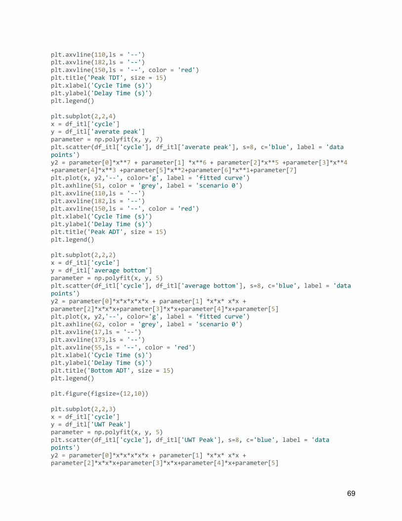
69

plt.axvline(110,ls = '--') plt.axvline(182,ls = '--') plt.axvline(150,ls = '--', color = 'red') plt.title('Peak TDT', size = 15) plt.xlabel('Cycle Time (s)') plt.ylabel('Delay Time (s)') plt.legend() plt.subplot(2,2,4) x = df_itl['cycle'] y = df_itl['averate peak'] parameter = np.polyfit(x, y, 7) plt.scatter(df_itl['cycle'], df_itl['averate peak'], s=8, c='blue', label = 'data points') y2 = parameter[0]*x**7 + parameter[1] *x**6 + parameter[2]*x**5 +parameter[3]*x**4 +parameter[4]*x**3 +parameter[5]*x**2+parameter[6]*x**1+parameter[7] plt.plot(x, y2,'--', color='g', label = 'fitted curve') plt.axhline(51, color = 'grey', label = 'scenario 0') plt.axvline(110,ls = '--') plt.axvline(182,ls = '--') plt.axvline(150,ls = '--', color = 'red') plt.xlabel('Cycle Time (s)') plt.ylabel('Delay Time (s)') plt.title('Peak ADT', size = 15) plt.legend() plt.subplot(2,2,2) x = df_itl['cycle'] y = df_itl['average bottom'] parameter = np.polyfit(x, y, 5) plt.scatter(df_itl['cycle'], df_itl['average bottom'], s=8, c='blue', label = 'data points') y2 = parameter[0]*x*x*x*x*x + parameter[1] *x*x* x*x + parameter[2]*x*x*x+parameter[3]*x*x+parameter[4]*x+parameter[5] plt.plot(x, y2,'--', color='g', label = 'fitted curve') plt.axhline(62, color = 'grey', label = 'scenario 0') plt.axvline(17,ls = '--') plt.axvline(173,ls = '--') plt.axvline(55,ls = '--', color = 'red') plt.xlabel('Cycle Time (s)') plt.ylabel('Delay Time (s)') plt.title('Bottom ADT', size = 15) plt.legend() plt.figure(figsize=(12,10)) plt.subplot(2,2,3) x = df_itl['cycle'] y = df_itl['UWT Peak'] parameter = np.polyfit(x, y, 5) plt.scatter(df_itl['cycle'], df_itl['UWT Peak'], s=8, c='blue', label = 'data points') y2 = parameter[0]*x*x*x*x*x + parameter[1] *x*x* x*x + parameter[2]*x*x*x+parameter[3]*x*x+parameter[4]*x+parameter[5]

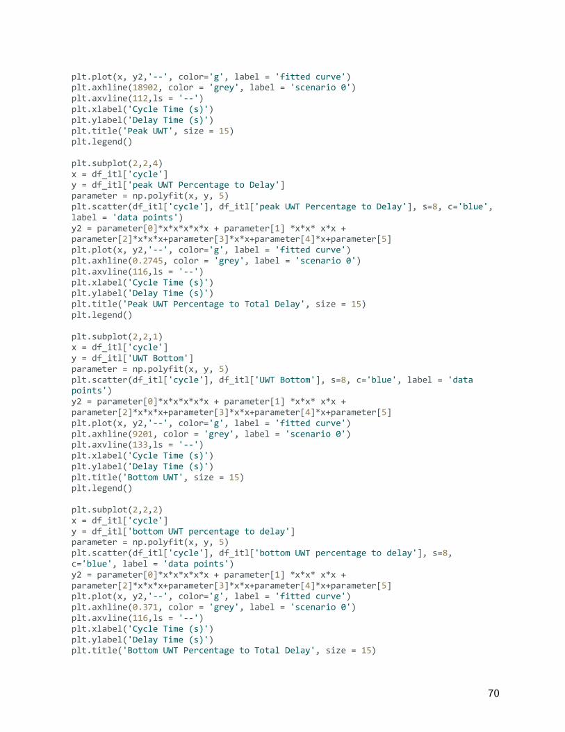
70

plt.plot(x, y2,'--', color='g', label = 'fitted curve') plt.axhline(18902, color = 'grey', label = 'scenario 0') plt.axvline(112,ls = '--') plt.xlabel('Cycle Time (s)') plt.ylabel('Delay Time (s)') plt.title('Peak UWT', size = 15) plt.legend() plt.subplot(2,2,4) x = df_itl['cycle'] y = df_itl['peak UWT Percentage to Delay'] parameter = np.polyfit(x, y, 5) plt.scatter(df_itl['cycle'], df_itl['peak UWT Percentage to Delay'], s=8, c='blue', label = 'data points') y2 = parameter[0]*x*x*x*x*x + parameter[1] *x*x* x*x + parameter[2]*x*x*x+parameter[3]*x*x+parameter[4]*x+parameter[5] plt.plot(x, y2,'--', color='g', label = 'fitted curve') plt.axhline(0.2745, color = 'grey', label = 'scenario 0') plt.axvline(116,ls = '--') plt.xlabel('Cycle Time (s)') plt.ylabel('Delay Time (s)') plt.title('Peak UWT Percentage to Total Delay', size = 15) plt.legend() plt.subplot(2,2,1) x = df_itl['cycle'] y = df_itl['UWT Bottom'] parameter = np.polyfit(x, y, 5) plt.scatter(df_itl['cycle'], df_itl['UWT Bottom'], s=8, c='blue', label = 'data points') y2 = parameter[0]*x*x*x*x*x + parameter[1] *x*x* x*x + parameter[2]*x*x*x+parameter[3]*x*x+parameter[4]*x+parameter[5] plt.plot(x, y2,'--', color='g', label = 'fitted curve') plt.axhline(9201, color = 'grey', label = 'scenario 0') plt.axvline(133,ls = '--') plt.xlabel('Cycle Time (s)') plt.ylabel('Delay Time (s)') plt.title('Bottom UWT', size = 15) plt.legend() plt.subplot(2,2,2) x = df_itl['cycle'] y = df_itl['bottom UWT percentage to delay'] parameter = np.polyfit(x, y, 5) plt.scatter(df_itl['cycle'], df_itl['bottom UWT percentage to delay'], s=8, c='blue', label = 'data points') y2 = parameter[0]*x*x*x*x*x + parameter[1] *x*x* x*x + parameter[2]*x*x*x+parameter[3]*x*x+parameter[4]*x+parameter[5] plt.plot(x, y2,'--', color='g', label = 'fitted curve') plt.axhline(0.371, color = 'grey', label = 'scenario 0') plt.axvline(116,ls = '--') plt.xlabel('Cycle Time (s)') plt.ylabel('Delay Time (s)') plt.title('Bottom UWT Percentage to Total Delay', size = 15)

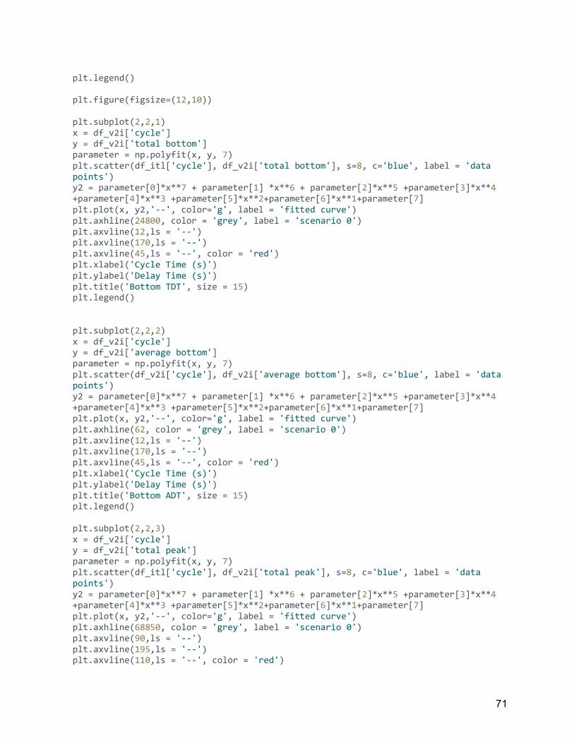
71

plt.legend() plt.figure(figsize=(12,10)) plt.subplot(2,2,1) x = df_v2i['cycle'] y = df_v2i['total bottom'] parameter = np.polyfit(x, y, 7) plt.scatter(df_itl['cycle'], df_v2i['total bottom'], s=8, c='blue', label = 'data points') y2 = parameter[0]*x**7 + parameter[1] *x**6 + parameter[2]*x**5 +parameter[3]*x**4 +parameter[4]*x**3 +parameter[5]*x**2+parameter[6]*x**1+parameter[7] plt.plot(x, y2,'--', color='g', label = 'fitted curve') plt.axhline(24800, color = 'grey', label = 'scenario 0') plt.axvline(12,ls = '--') plt.axvline(170,ls = '--') plt.axvline(45,ls = '--', color = 'red') plt.xlabel('Cycle Time (s)') plt.ylabel('Delay Time (s)') plt.title('Bottom TDT', size = 15) plt.legend() plt.subplot(2,2,2) x = df_v2i['cycle'] y = df_v2i['average bottom'] parameter = np.polyfit(x, y, 7) plt.scatter(df_v2i['cycle'], df_v2i['average bottom'], s=8, c='blue', label = 'data points') y2 = parameter[0]*x**7 + parameter[1] *x**6 + parameter[2]*x**5 +parameter[3]*x**4 +parameter[4]*x**3 +parameter[5]*x**2+parameter[6]*x**1+parameter[7] plt.plot(x, y2,'--', color='g', label = 'fitted curve') plt.axhline(62, color = 'grey', label = 'scenario 0') plt.axvline(12,ls = '--') plt.axvline(170,ls = '--') plt.axvline(45,ls = '--', color = 'red') plt.xlabel('Cycle Time (s)') plt.ylabel('Delay Time (s)') plt.title('Bottom ADT', size = 15) plt.legend() plt.subplot(2,2,3) x = df_v2i['cycle'] y = df_v2i['total peak'] parameter = np.polyfit(x, y, 7) plt.scatter(df_itl['cycle'], df_v2i['total peak'], s=8, c='blue', label = 'data points') y2 = parameter[0]*x**7 + parameter[1] *x**6 + parameter[2]*x**5 +parameter[3]*x**4 +parameter[4]*x**3 +parameter[5]*x**2+parameter[6]*x**1+parameter[7] plt.plot(x, y2,'--', color='g', label = 'fitted curve') plt.axhline(68850, color = 'grey', label = 'scenario 0') plt.axvline(90,ls = '--') plt.axvline(195,ls = '--') plt.axvline(110,ls = '--', color = 'red')

72

plt.title('Peak TDT', size = 15) plt.xlabel('Cycle Time (s)') plt.ylabel('Delay Time (s)') plt.legend() plt.subplot(2,2,4) x = df_v2i['cycle'] y = df_v2i['averate peak'] parameter = np.polyfit(x, y, 7) plt.scatter(df_itl['cycle'], df_v2i['averate peak'], s=8, c='blue', label = 'data points') y2 = parameter[0]*x**7 + parameter[1] *x**6 + parameter[2]*x**5 +parameter[3]*x**4 +parameter[4]*x**3 +parameter[5]*x**2+parameter[6]*x**1+parameter[7] plt.plot(x, y2,'--', color='g', label = 'fitted curve') plt.axhline(51, color = 'grey', label = 'scenario 0') plt.axvline(90,ls = '--') plt.axvline(195,ls = '--') plt.axvline(110,ls = '--', color = 'red') plt.xlabel('Cycle Time (s)') plt.ylabel('Delay Time (s)') plt.title('Peak ADT', size = 15) plt.legend() plt.figure(figsize=(12,10)) plt.subplot(2,2,3) x = df_v2i['cycle'] y = df_v2i['UWT Peak'] parameter = np.polyfit(x, y, 7) plt.scatter(df_itl['cycle'], df_v2i['UWT Peak'], s=8, c='blue', label = 'data points') y2 = parameter[0]*x**7 + parameter[1] *x**6 + parameter[2]*x**5 +parameter[3]*x**4 +parameter[4]*x**3 +parameter[5]*x**2+parameter[6]*x**1+parameter[7] plt.plot(x, y2,'--', color='g', label = 'fitted curve') plt.axhline(18902, color = 'grey', label = 'scenario 0') plt.axvline(112,ls = '--') plt.xlabel('Cycle Time (s)') plt.ylabel('Delay Time (s)') plt.title('Peak UWT', size = 15) plt.legend() plt.subplot(2,2,4) x = df_v2i['cycle'] y = df_v2i['peak UWT Percentage to Delay'] parameter = np.polyfit(x, y, 7) plt.scatter(df_v2i['cycle'], df_v2i['peak UWT Percentage to Delay'], s=8, c='blue', label = 'data points') y2 = parameter[0]*x**7 + parameter[1] *x**6 + parameter[2]*x**5 +parameter[3]*x**4 +parameter[4]*x**3 +parameter[5]*x**2+parameter[6]*x**1+parameter[7] plt.plot(x, y2,'--', color='g', label = 'fitted curve') plt.axhline(0.2745, color = 'grey', label = 'scenario 0') plt.axvline(97,ls = '--') plt.xlabel('Cycle Time (s)')

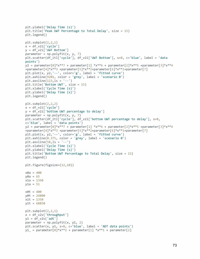
73

plt.ylabel('Delay Time (s)') plt.title('Peak UWT Percentage to Total Delay', size = 15) plt.legend() plt.subplot(2,2,1) x = df_v2i['cycle'] y = df_v2i['UWT Bottom'] parameter = np.polyfit(x, y, 7) plt.scatter(df_itl['cycle'], df_v2i['UWT Bottom'], s=8, c='blue', label = 'data points') y2 = parameter[0]*x**7 + parameter[1] *x**6 + parameter[2]*x**5 +parameter[3]*x**4 +parameter[4]*x**3 +parameter[5]*x**2+parameter[6]*x**1+parameter[7] plt.plot(x, y2,'--', color='g', label = 'fitted curve') plt.axhline(9201, color = 'grey', label = 'scenario 0') plt.axvline(123,ls = '--') plt.title('Bottom UWT', size = 15) plt.xlabel('Cycle Time (s)') plt.ylabel('Delay Time (s)') plt.legend() plt.subplot(2,2,2) x = df_v2i['cycle'] y = df_v2i['bottom UWT percentage to delay'] parameter = np.polyfit(x, y, 7) plt.scatter(df_itl['cycle'], df_v2i['bottom UWT percentage to delay'], s=8, c='blue', label = 'data points') y2 = parameter[0]*x**7 + parameter[1] *x**6 + parameter[2]*x**5 +parameter[3]*x**4 +parameter[4]*x**3 +parameter[5]*x**2+parameter[6]*x**1+parameter[7] plt.plot(x, y2,'--', color='g', label = 'fitted curve') plt.axhline(0.371, color = 'grey', label = 'scenario 0') plt.axvline(58,ls = '--') plt.xlabel('Cycle Time (s)') plt.ylabel('Delay Time (s)') plt.title('Bottom UWT Percentage to Total Delay', size = 15) plt.legend() plt.figure(figsize=(12,10)) x0a = 400 y0a = 65 x1a = 1350 y1a = 51 x0t = 400 y0t = 24800 x1t = 1350 y1t = 68850 plt.subplot(2,2,1) x = df_v2v['throughput'] y1 = df_v2v['adt'] parameter = np.polyfit(x, y1, 2) plt.scatter(x, y1, s=8, c='blue', label = 'ADT data points') y1_ = parameter[0]*x**2 + parameter[1] *x**1 + parameter[2]

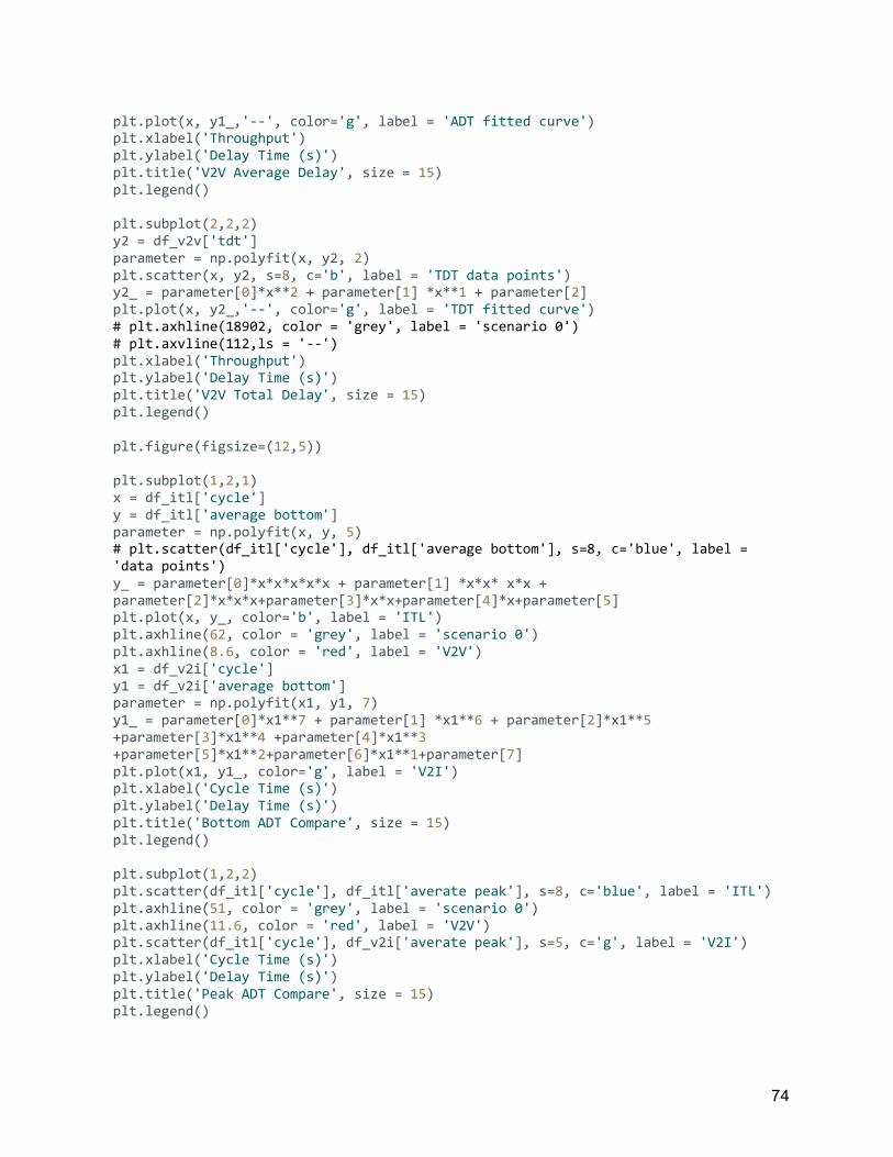
74

plt.plot(x, y1_,'--', color='g', label = 'ADT fitted curve') plt.xlabel('Throughput') plt.ylabel('Delay Time (s)') plt.title('V2V Average Delay', size = 15) plt.legend() plt.subplot(2,2,2) y2 = df_v2v['tdt'] parameter = np.polyfit(x, y2, 2) plt.scatter(x, y2, s=8, c='b', label = 'TDT data points') y2_ = parameter[0]*x**2 + parameter[1] *x**1 + parameter[2] plt.plot(x, y2_,'--', color='g', label = 'TDT fitted curve') # plt.axhline(18902, color = 'grey', label = 'scenario 0') # plt.axvline(112,ls = '--') plt.xlabel('Throughput') plt.ylabel('Delay Time (s)') plt.title('V2V Total Delay', size = 15) plt.legend() plt.figure(figsize=(12,5)) plt.subplot(1,2,1) x = df_itl['cycle'] y = df_itl['average bottom'] parameter = np.polyfit(x, y, 5) # plt.scatter(df_itl['cycle'], df_itl['average bottom'], s=8, c='blue', label = 'data points') y_ = parameter[0]*x*x*x*x*x + parameter[1] *x*x* x*x + parameter[2]*x*x*x+parameter[3]*x*x+parameter[4]*x+parameter[5] plt.plot(x, y_, color='b', label = 'ITL') plt.axhline(62, color = 'grey', label = 'scenario 0') plt.axhline(8.6, color = 'red', label = 'V2V') x1 = df_v2i['cycle'] y1 = df_v2i['average bottom'] parameter = np.polyfit(x1, y1, 7) y1_ = parameter[0]*x1**7 + parameter[1] *x1**6 + parameter[2]*x1**5 +parameter[3]*x1**4 +parameter[4]*x1**3 +parameter[5]*x1**2+parameter[6]*x1**1+parameter[7] plt.plot(x1, y1_, color='g', label = 'V2I') plt.xlabel('Cycle Time (s)') plt.ylabel('Delay Time (s)') plt.title('Bottom ADT Compare', size = 15) plt.legend() plt.subplot(1,2,2) plt.scatter(df_itl['cycle'], df_itl['averate peak'], s=8, c='blue', label = 'ITL') plt.axhline(51, color = 'grey', label = 'scenario 0') plt.axhline(11.6, color = 'red', label = 'V2V') plt.scatter(df_itl['cycle'], df_v2i['averate peak'], s=5, c='g', label = 'V2I') plt.xlabel('Cycle Time (s)') plt.ylabel('Delay Time (s)') plt.title('Peak ADT Compare', size = 15) plt.legend()

-how new technologies impact a conventional intersection

Documents