How Much Did the US Government Value its Troops’ Lives in World War II?: Evidence from Dollar-Fatality Tradeoffs in Land Battles

Chris Rohlfs1

18 January 20052

PRELIMINARY AND INCOMPLETE

Abstract

This study uses battle-level data to estimate the rate at which the US Army traded dollars for fatalities in World War II. Using data from 164 engagements, I estimate the effects American and German troops and tanks on mission accomplishment and US battle fatalities. I supplement these data with cost estimates compiled from archived US Army records. I find that the Army could have reduced fatalities by increasing its use of tanks and decreasing its use of ground troops. In 2003 dollars, my preferred estimates suggest that this policy would have cost $1 million to $2 million per life saved. This figure appears roughly similar to soldiers’ own willingness-to-pay to avoid fatality risk.

1 Department of Economics. University of Chicago. 1126 E. 59th St. Chicago IL. 60637. email: car@uchicago.edu 2 This research was made possible in part by generous support by the National Institute for Aging. Special thanks to Chris Lawrence and Richard Anderson of the Dupuy Institute for their help and guidance. Thanks also to Mark Duggan, Michael Greenstone, Steve Levitt, Casey Mulligan to numerous other colleagues for many helpful comments, and to countless members of the defense community who freely offered contacts, information, and insights.

1

“[The continuing decline in the proportion of combat troops to the total Army is] due to the mechanization of the Army, i.e., the great masses of armor and airplanes that prepare the way for the final assault of the foot soldier with the resultant saving of human life.”3

Many government policies exist to prevent premature deaths and to extend citizens’ lives.

A large literature exists in economics exploring these policies and relating fatality risks to dollar

costs. Viscusi (1996) finds considerable variation in the cost per life saved for different life-

saving government policies. In 2003 dollars, the policies he examines range in cost from $0.2

million to $130 billion per life saved. Holding constant the amount spent saving lives,

economists argue, the government could save many more lives by allocating these expenditures

more efficiently. For each life that is not saved at $130 billion a piece, the government can save

650,000 lives at $0.2 million a piece. Some government agencies have responded to this

criticism by adopting their own dollar valuations of fatality risk. The US Environmental

Protection Agency removes arsenic from drinking water until the costs exceed $6.1 million per

life. The US Department of Transportation improves roads until the costs exceed $3 million per

life.4

In this study, I measure dollar-fatality tradeoffs faced by the US military in World War II.

Defense constitutes one of the largest categories of public expenditure, both in the US and in the

rest of the world. In 1997, world defense expenditure totaled $0.93 trillion – equaling 2.5% of

world GNP and 10% of expenditure by central governments.5 In addition to these dollar

expenditures, wars involve large non-monetary costs, including human casualties and the

disruption of lives. Military policies have far-reaching effects, and the worst mistakes in military

3 Operations Division, War Department General Staff, May 1945. Quoted in Greenfield, Palmer, and Wiley (1947, pg. 255). General Stillwell appealed to the General Staff to increase the size of the ground army to avoid disaster in Japan. Chief of Staff General Marshall asked the Operations Division to compose a reply, which is quoted here. 4 EPA and DOT figures taken from Holt (2004). 5 By comparison, world public expenditure on education (the largest category) totaled $1.6 trillion/year. Data sources: US State Department (1999) and United Nations (2000). I use 1997 because this is the most recent year for which UNESCO provides world education expenditure estimates. All dollar figures in this paper have been inflated to 2003 dollars using the Consumer Price Index.

2

policy can be catastrophic. Throughout the history of modern warfare, armies have made

tradeoffs between armor expenditures and fatality risk.6 Explicitly measuring dollar-fatality

tradeoffs is one prudent, systematic, and transparent way to help military planners make difficult

and necessary decisions.

In World War II, the US Army sent 16 armored divisions and 47 infantry divisions to the

Western Front.7 As Table 1 shows, the average infantry division sent to the Western Front

included 66 tanks and 14,400 troops. The average armored division was considerably more

tank-intensive, with 281 tanks and only 11,500 troops.8 By using more troops, infantry

divisions put more soldiers’ lives at risk, and these units suffered more fatalities. Armored

divisions, on the other hand, cost considerably more money. Had the Army replaced some of its

infantry divisions with armored divisions, it could have reduced US battle fatalities. However,

doing so would have cost the Army more money. The goal of this paper is to measure how

much money such a policy would have cost the US Army per life saved.

Over the course of the war, the average infantry division suffered 2,077 battle-related

fatalities, while the average armored division suffered only 825.9 To mobilize the average

infantry division and operate and maintain it over the war cost roughly $2.1 billion. For the

average armored division, mobilization, operation, and maintenance cost a total of roughly $3.1

billion. Later in this paper, I attempt to precisely estimate the cost of reducing US fatalities,

controlling for various possible confounding factors. However, we can roughly estimate this

6 These tradeoffs continue to be relevant today (Banerjee and Hart (2004), Schmitt (2004)). 7 Data source: Stanton (1984), pp. 47-182. 8 Many of the armored division’s troops served in administrative, supply, and technical roles. Consequently, the “rifle strength” of the armored division was much lower than that of the infantry division. Anderson (2000); Greenfield, Palmer, and Wiley (1947), pg. 334. The killed and wounded figures in Table 1 only include casualties suffered by the organic unit. That is, they do not include casualties suffered by attached units. The troops, tanks, and dollar cost figures in Table 1 refer to the organic unit as well. The engagement-level data used later in the paper include troops, tanks, and casualties for the organic unit plus attachments. The dollar costs are adjusted accordingly. 9 As Table 1 shows, nonfatal injuries were also higher for infantry divisions.

3

cost by simply comparing average fatalities and dollar costs between infantry and armored

divisions. 10 On average, armored divisions cost roughly $1.0 billion more than infantry

divisions, and they experienced 1,252 fewer fatalities. Hence, by replacing infantry divisions

with armored divisions, the Army could have reduced fatalities at a cost of about $0.8 million

per life.

When the government spends money to reduce fatalities, it is making in-kind

contributions to its citizens. Economists argue that citizens themselves are the ones best

equipped to assess the dollar value of such contributions. They contend that, when making

dollar-fatality tradeoffs, the government should purchase just as many fatality reductions as

citizens would purchase on their own. Any additional fatality reductions are appreciated by the

citizens, but they would be happier to just receive the cash (i.e., lower taxes). A large literature

exists in economics measuring citizens’ own willingness-to-pay for reductions in fatality risk.

Viscusi (1993) provides a useful review. To compare the cost of saving troops’ lives with

citizens’ willingness-to-pay, this paper relies on willingness-to-pay estimates from Costa and

Kahn (2004).

The cost per life saved estimates in this paper rely on data from a variety of sources. To

measure expenditures, I assembled an assortment of archived records the US Army and other

branches of government.11 Using these data, I estimate the pay, training, equipment,

10 Infantry divisions and armored divisions served distinct purposes in combat. As I discuss later in the paper, tank intensity correlates strongly with some other important determinants of mission success and casualties. I adjust for many of these factors later in the paper and obtain similar estimates for the cost per life saved. Hence, the dollar-fatality tradeoffs shown here are probably not driven by omitted variables. These large fatality and cost differences are probably attributable to characteristics about the divisions themselves – e.g., the numbers of troops and tanks. Hence, any new armored divisions that the Army mobilized would probably resemble the average armored division in terms of fatalities and dollar costs. Similarly, the infantry divisions that they replaced would probably resemble the average infantry division. 11 Obtained primarily from Modern Military Records at National Archives II in College Park, MD and the Center for Military History in Washington, DC. Other sources include US Congressional Statues and historical US Budget reports.

4

maintenance, food, clothing, ammunition, gasoline, and transportation costs associated with

infantry and armored divisions. I relate these expenditures to combat outcomes by estimating

the effects of US troops and tanks on mission accomplishment and battle fatalities. I estimate

these combat effects with data from 164 division-level, 1- to 12-day engagements from the

Western Front in World War II. The Dupuy Institute and Colonel Trevor Dupuy’s Historical

Evaluation and Research Organization compiled these data from American and German primary

sources. The data describe each side’s troops, tanks, and fatalities, and they include indices for

mission accomplishment, terrain, weather, and human factors.

The primary objective of this paper is to provide information about the relationship

between public and private valuations of fatality risk. I focus on one specific type of public

sector activity (defense) that involves dollar-fatality tradeoffs on a large scale. As an added

benefit, this study provides information about costs for a large area of public expenditure –

military operations. Such estimates, together with studies of the benefits of military operations,

could help policymakers determine whether specific military activities are worth the costs.

Previous studies of the effects of troops on casualty effectiveness have generally obtained

mixed and unstable results. A handful of researchers have discussed possible explanations for

this finding.12 I propose a novel explanation to this puzzling finding from the literature – that

increasing own troops increases own casualties. I argue that governments willingly sent troops

into combat and accepted higher casualties as costs of accomplishing military objectives.13 In

2003 dollars, my preferred estimates suggest that reducing fatalities would have cost the US

Army $1 million to $2 million per life. Given real income levels at the time, these estimates are

comparable to what we might expect soldiers’ willingness-to-pay to have been. However, I find

12 See, for instance, Hartley (2001), Helmbold (1993), and Dupuy (1977). 13 Similarly, Lawrence (1996) discusses retreat as one way in which a fighting unit can reduce its casualties.

5

considerable variation in the cost per life saved across different situations. Hence, the

government appears to have valued lives appropriately on average. I find many specific

situations, however, in which the government appears to have overvalued or undervalued

soldiers’ lives.

The structure of the paper proceeds as follows. Section II describes some key factors

determining the US Army’s use of tanks in World War II. In Section III, I describe the data

used in this analysis, and I show some simple empirical relationships from the combat data. In

Section IV, I develop an economic model in which governments balance mission objectives

against monetary and non-monetary costs. In Section V includes empirical results from this

model and estimates of the cost per life saved for the US Army. I explore how this cost varied

across different situations, and I examine the sensitivity of the results to model misspecification.

In Section VI, I discuss the implications of these results for public policy. Section VII

concludes and is followed by a Data Appendix.

II. Key Institutional Factors

A. The Adoption of Tanks in the US Army

After World War I, British military theorists advocated increasing the use of tanks to

avoid the casualty-intensive stalemate of trench warfare.14 Colonel J.F.C. Fuller and Captain

B.H. Liddell Hart argued that using tanks could reduce battle casualties:

“[In] the first battle of Somme, our casualties per square mile of battlefield gained were 5,300; during the same months in 1917, at the third battle of Ypres, they were 8,200; and during the same period in 1918 they were 83. In the third period alone were tanks used in numbers and efficiently.”15

14 Wilson (1998), pg. 120. Liddell Hart (1925), pp. 66-77. Fuller (1928), pp. 106-151. 15 Fuller (1928), pg. 129.

6

Fuller and Liddell Hart’s ideas were influential both in the US Army and in Congress.16

However, the US Army was slow to adopt tanks due to conservatism, cronyism, and lack of

vision among high-ranking Army personnel.17 From World War I through the early part of

World War II, US tank technology lagged behind that of the other European powers. After

conducting large-scale field exercises in 1940, Army officials concluded that the tank would play

a larger role than previously thought.18 The US Army mobilized its first armored division in July

1940.19 However, the use of armor still met with stiff resistance from both the Chief of Staff and

the Commander of Army Ground Forces.20 Their criticisms arose in large part due to budget

constraints imposed by Congress and the civilian War Production Board.21

The Army’s budget and the number of available draftees were largely determined by

civilian branches of government. During the interwar period, Congressional budget cuts

seriously constrained the size of the military and the development of the tank.22 By the time

Congress expanded the budget in the early 1940s, wartime production was constrained by the

physical capacity of the US economy.23 Physical factors also severely constrained the number of

troops that the Army could draft.24 Nevertheless, many non-physical factors also affected Army

procurement. When calculating the feasibility of wartime procurement objectives, the War

16 Representative Ross Collins of Mississippi, Chairman of the US House Subcommittee on Military Appropriations, enthusiastically promoted Fuller and Liddell Hart’s ideas: “Foot troops should be provided with adequate means of protecting themselves against tanks, and, of course, the obvious means is the protection given by the armor of tanks. Soldiers with nothing to protect them but khaki are virtually asked to commit suicide.” US Seventy-Second Congress (1932), pg. 9932. 17 Steadman (1982). James (1970), pp. 356-357. Watson (1950), pp. 15-50. 18 Germany’s swift defeat of France in June reinforced this view. 19 Wilson (1997), pp. 147-150. 20 Greenfield, Palmer, and Wiley (1947), pp. 334-335; Steadman (1982). 21 Steadman (1982), Smith (1959), pp. 154-158. 22 Steadman (1982). Green, Thompson, and Roots (1955), pg. 30. 23 In September 1942, the famous economist Simon Kuznets submitted a report questioning the physical feasibility of the War Department’s production goals. His report claimed that it was not physically possible for the US economy to meet the production demands of the Victory Program. Kuznets’s report led to drastic reductions in Army spending plans (Smith, 1959, pp. 154-158). 24 The troop basis for the original Victory Program counted on the “maximum number of troops available to the Army.” Smith (1959), pg. 136.

7

Production Board also considered “the needs of the civilian and industrial economy.”25 In

response to public sympathy, Congress limited the Army’s ability to draft 18-year-olds and

fathers. The restrictions they placed varied over time, depending on the needs of the war effort.26

B. Determinants of Tank Intensity in Battle

In 1942, the first infantry divisions that the US Army sent abroad included 15,514 troops

and 0 tanks. The first armored divisions included 14,620 troops and 390 tanks. In September

1943, the US cut its armored division’s tanks by nearly a third to 263.27 The excess tanks were

used to attach a 76-tank, 750-troop tank battalion to nearly every US infantry division.28 In

practice, US Army divisions did not strictly adhere to their prescribed Tables of Organization

and Equipment. Unit commanders attached artillery and tank destroyer battalions to different

divisions as necessary.29 Later in the war, economic factors forced many divisions on both sides

to fight with less than the prescribed number of tanks.30

Infantry and armored divisions typically traveled together in corps of 2 to 4 divisions.31

US tank doctrine recommended that infantry divisions attack the enemy first to create an opening

in the enemy’s front lines. Armored forces would then exploit this opening and penetrate deep

into enemy territory, staging swift attacks in the rear of enemy forces. In practice, however, the

25 Smith (1959, pg. 154). Colonel Lewis Sanders commented on this issue in a Congressional Hearing: “[The British] have cut out many services which we have not cut out. For instance, when I was in New York I saw a man operating a sightseeing bus.” (US Seventy-Eighth Congress, 1943, pg. 197). 26 Palmer, Wiley, and Keast (1959), pp. 201-207. Greenfield, Palmer, and Wiley (1947), pp. 246-251. 27 McNair’s plan also removed administrative and supply elements from the division, cutting the personnel size to 10,937 (Wilson, 1997, pp. 182-187). In practice, the Army attached quartermaster and headquarters companies to these divisions which ended up serving the same functions (Anderson, 2000). 28 Stanton (1984), pg. 19. Greenfield, Palmer, and Wiley (1947), pg. 333. 29 The tank destroyer, or a self-propelled artillery piece, was similar in function and usefulness to a standard artillery piece. Anderson (2000), Gabel (1985a). The 1st Armored and 3rd and 34th Infantry Divisions avoided the 1943 reorganization until summer 1944, because they were in combat. The 2nd and 3rd Armored Divisions avoided the 1943 reorganization altogether. Greenfield, Palmer, and Wiley (1947), pg. 333; Wilson (1997), pg. 187; Stanton (1984), pp. 47-51. 30 Anderson (2000). This situation was particularly severe for the Germans (Gabel, 1985b, pg. 8). 31 Kahn and McLemore (1980) pp. 192-199.

8

armored division rarely traveled more than a few miles from the other elements of the corps.32

Infantry divisions spent more days in combat than armored divisions did.33 However, armored

divisions’ mobility allowed them to fight many high-value missions and to provide

reinforcements to other divisions.34

Armored divisions could travel quickly across open terrain. However, many adverse

circumstances could hinder armored divisions’ movements. Some infantry divisions ventured

into the center of the Italian peninsula, but the region’s mountainous terrain confined the

armored divisions to coastal areas.35 Adverse terrain and thick vegetation often forced tanks to

travel on roads, which were particularly vulnerable to obstacles and ambushes.36 River crossings

took longer for armored divisions than for infantry, because of the time it took for their engineers

to build heavy bridges.37 Beach landings also posed a problem for tanks.38 One of the most

important issues constraining tank movement, however, was gasoline.39 Factors such as these

32 Patton noted this himself in describing the 1st Armored Division’s activities in Italy (Greenfield, Palmer, and Wiley, 1947, pg. 332). One notable exception is the US 4th Armored Division’s campaign in Lorraine in late 1944, described in detail in Gabel (1985b, 1986). 33 202 days for infantry versus 118 days for armored. Data sources: Ruppenthal (1959, pp. 282-283) and US Army Historical Services Division (1962). Data for combat days are missing for the US 1st Armored and 85th Infantry Divisions.34 One famous such case is the 4th and 10th Armored Divisions’ relief of the 101st Airborne Division in Bastogne in December 1944. The Army designed and experimented with a handful of highly mobile motorized infantrydivisions early in the war. However, Army commanders felt that these divisions were not sufficiently effective in combat to justify their requirements for gasoline and other resources (Greenfield, Palmer, and Wiley 1947, pp. 337-339). 35 Many infantry divisions traveled along the coast as well. US II Corps and VI Corps (all infantry) traveled straight through the center of the peninsula. The British 1st and 7th Armored Divisions traveled parallel routes northwest along the opposite coasts (Pimlott, 1995, pp. 140-145, Evans, 2002, pg. 44). 36 Gabel (1985b), pg. 24; Gabel (1986), pg. 8. In February 1944, soft ground slowed the Axis advance toward Allied forces at Anzio, forcing the tanks to travel by road (Evans, 2002, pp. 49-50). At Normandy, along the eastern edge of the D-Day landings, traffic jams prevented Allied armor from supporting the British 185th Infantry Brigade (Evans, 2002, pg. 55). 37 Gabel (1986), pg. 12. 38 A considerable number of Allied tanks capsized in rough waters during the D-Day landings (Evans, 2002, pg. 54; The Dupuy Institute (2001b), pp. 65-68. 39 In summer 1942, Rommel’s armored forces had extended more than 600 miles from his main supply base in Tripoli out to western Egypt. The gasoline-starved Afrika Korps could not afford the luxury of strategic pauses when they hastily attacked British forces in Alam Halfa (Pimlott, 1995, pg. 106; Liddel-Hart, Bayerlein, and Roberts, 1956, pp. 19-20; Dupuy, 1962b, pp. 34-35). Shortages in gasoline also placed considerable constraints on the progress of Patton’s 3rd Army (which included 3 armored divisions) in Lorraine in 1944. Gasoline was abundant

9

often prevented armored forces from staging attacks or forced infantry to fight without

supporting armor.

III. Data and Descriptive Evidence

A. The Land Warfare Database and The Division-Level Engagement Database

The combat data used in this analysis describe 164 land battles fought on the Western

Front between 1942 and 1945. These data come from the Division-Level Engagements Database

and its predecessor, the Land Warfare Database.40 Both datasets were compiled from archived

American and German primary sources such as unit histories and after action reports. The Land

Warfare Database is publicly available. The Division-Level Engagements Database is

proprietary and may be acquired at a cost from The Dupuy Institute. In addition to these combat

data, this study relies upon a wide range of archival sources describing the costs of military

operations. I describe these sources in the Data Appendix.

In total, the Division-Level Engagements Database and the Land Warfare Database

include 230 engagements between American and German forces in World War II.41 Across

these 230 engagements, the number of American troops ranges from 190 to 126,000. That is,

large variation exists in the scale at which these engagements were measured. When all of these

engagements are included in the sample, the scale of the battle – which is highly correlated with

troops, tanks, and fatalities – tends to drive all the results. That is, in the larger sample, troops

in Normandy, but the 500 mile supply lines could only keep the 3rd Army at ¼ of its regular supply. Eisenhower had also given priority for supplies to Allied forces further north (Gabel, 1985b, pg. 6). Had ample gasoline existed, Patton’s forces would have pursued a more aggressive course toward Germany. Instead, the 3rd Army fought a mainly static war of attrition in Lorraine. Gabel (1986, pg. 23). 40 The Division-Level Engagements Database is constructed and maintained by The Dupuy Institute. The Land Warfare Database was constructed in the 1960s and 1970s by Colonel Trevor Dupuy’s Historical Evaluation and Research Organization. The Division-Level Engagements Database constitutes an updated and expanded version of the Land Warfare Database. Both datasets were constructed with support from the US Army Center for Army Analysis. 41 Both datasets contain many other engagements from other wars and countries. However, the data in this paper are limited to US-German battles from World War II.

10

and tanks are both positively correlated with fatalities. However, these positive relationships are

primarily driven by the fact that some battles were large and some were small. While the scale

of combat is an interesting variable, the focus of this paper is the substitution between armored

and infantry divisions of similar size. Consequently, I restrict the sample to 164 observations

that are measured at the division-level.42 These engagements include between 8,300 and 32,000

troops.43 Of the 164 engagements used in this analysis, 39 appear in both the Division-Level

Engagements Database and the Land Warfare Database. In the cases in which the 2 datasets

disagree, I use the updated data (from the Division-Level Engagements Database). Of the

remaining 125 observations, 5 come from the Land Warfare Database and 120 come from the

Division-Level Engagements Database.

In the 164-engagement dataset, roughly 47% of the observations (77 engagements) come

from North Africa and Italy. The remaining 87 engagements involve American divisions that

entered Europe from Northern France and traveled eastward into Germany. In the 164 battles,

roughly 1,500 Americans were killed in action in the Mediterranean Theater and 1,600 in the

European Theater. These battles account for roughly 4% of Americans killed in action in the

Mediterranean Theater and roughly 2% in the European Theater.44

42 If more precise data were available, many of the larger, corps-level engagements could be broken down into smaller, division-level engagements. These large observations tend to rely on rough estimates. Many of the smaller, battalion-level engagements provide incomplete measures of the number of troops available to the unit for administration, supply, and reserves. Hence, the troop measurements for these extreme observations may not be comparable to the troop measurements in the rest of the dataset. When all 230 observations are included in the data, the coefficient on troops is extremely unstable across specifications. Using this full sample, I obtain cost per life saved estimates ranging from -$2.1 million to $0.0 million, as described in the sensitivity analysis. 43 I define an engagement to be division-level if the US force’s name is coded in the data as the full division. An additional 5 observations (4 small and 1 large) are dropped because the observations are effectively regiment-level or corps-level. The numbers of US troops for these 5 engagements are 3,900, 4,800, 5,000, 5,600, and 44,000, respectively. When these 5 engagements are included in the data, I obtain cost per life saved estimates of -$0.2 million to $2.9 million. The one negative value appears in the specification with no controls. 44 Data sources: Division-Level Engagement Database; US Army Adjutant General (1953) pp. 84-89. The representativeness of the Division-Level Engagement Database is discussed in detail in The Dupuy Institute (2005). For more information on these specific campaigns, see Dupuy (1962a), Dupuy (1962b), Evans (2002), and Pimlott (1995).

11

I focus on the Western Front of World War II for a variety of reasons. By confining the

analysis to a small series of campaigns, the estimates in this study pertain to a specific set of

government policies. Consequently, these estimates can be interpreted as the value a particular

government placed on avoiding fatalities in a particular war. Differences in force sizes and

compositions across different wars are likely to be related to many other variables that influence

combat outcomes. By limiting the sample in this way, I avoid many potential sources of bias in

estimating combat effects. World War II is a modern war in which tanks and airplanes were

used extensively. Unlike most modern wars, however, many declassified records exist for both

sides, allowing for a moderately-sized sample of battles. The combat data available for the

Western Front of World War II are precisely measured and they all come from detailed primary

sources. Moreover, a wide range of archived US Army records exists documenting the costs,

expenditures, and policymaking process.

The data used in this study include directly observable variables and a range of indices

representing experts’ judgments about “human factors” in battle. The objective data on inputs

describe both sides’ force strengths and casualties – both for troops and equipment.45 All 164

observations include data on total human casualties (i.e., soldiers killed, wounded, and missing

or captured). However, only 102 include disaggregated measurements of the numbers of US

troops killed in action or wounded in action. For the remaining 62 observations, I estimate killed

in action and wounded in action as 0.12 and 0.63 times total casualties, respectively.46 The

equipment measured includes artillery pieces, tanks, and aerial sorties in close combat (fighters

45 However, the data contain many missing values for equipment losses. 46 These numbers are the fraction of casualties killed in action and the fraction wounded in action, calculated from the 102-engagement subsample. For German casualties, these fractions are 0.11 and 0.32, respectively. It is well known among empirical economists that measurement error in the dependent variable does not cause bias. Using the 102-engagement subsample, without controlling for human factors, I obtain cost per life saved estimates ranging from $0.3 million to $1.3 million. However, after controlling for human factors, the estimates (particularly the effects of tanks) become very unstable due to the low numbers of degrees of freedom. After controlling for human factors in the 102-engagement subsample, I obtain cost per life saved estimates of -$1.8 million to -$2.4 million.

12

and bombers together).47 The data also include descriptive variables such as the duration of

fighting, the width of the attacking force,48 and terrain and weather factors. The subjective data

include continuous 0 to 1 indices for human factors influencing combat outcomes. These indices

measure defensive fortifications and attacker’s advantage in leadership, intelligence, planning,

reserves, training, force quality, morale, and air superiority. One additional judgment variable I

use is an index measuring the degree to which the attacking unit accomplished its mission.49

This mission accomplishment index is one of the main dependent variables used in this study. I

describe how this variable is constructed in the Data Appendix. The degree of mission

accomplishment summarizes a variety of factors including miles advanced and targets destroyed.

This subjective mission accomplishment index appears to be the best way to measure the overall

effectiveness of a military operation.50

In addition to these variables, the empirical analysis in this paper relies on 3 variables

constructed by the researcher. The first 2 are dummies for whether the engagement occurred at a

47 These input variables measure the quantities at the start of the battle, or “feeding strengths” for the respective armies. About 24% of the American tanks used are light tanks. For the purposes of this analysis, I ignore the distinction between light and heavy tanks. As I show in the sensitivity analysis, ignoring light tanks does not change the results of this study. In 115 of the 164 battles, at least one side’s aerial sorties contain missing observations. Richard Anderson of The Dupuy Institute, in a private conversation, indicated that these observations are probably zeros. A handful of other forms of imputation were used sparingly by The Dupuy Institute in coding the primary records. Descriptions of the sources and imputation appear in the “remarks” field in the raw data. 48 Duration measured in days. Width measured in kilometers. 49 I normalize the terrain, weather, human factor, and mission accomplishment indices in this study so that they all range from 0 to 1. I exclude a handful of human factors from the regressions: initiative, technology, mobility, maneuver, momentum, force depth, and logistics. I exclude surprise, initiative and momentum because they relate to choices that may depend on troops and tanks. I exclude technology, mobility, and maneuver because these are fundamental characteristics about the number of troops and tanks. Hence, they should not be held constant when measuring troops’ and tanks’ effects. Similarly, given force size, force depth provides information about the density of the unit – which might vary based on the number of tanks. I include the existence of reserve forces as a control because these might have influenced the opponent’s behavior. I exclude logistics as a control variable largely because many supply problems are caused by the gasoline demands of tanks. Supply shortages may have affected other combat inputs such as ammunition, food, and other equipment. However, these effects were probably minor compared to the large effect that supply shortages had on the shadow price of tanks. 50 I reproduce the results of this study using 2 other, less subjective measures of mission accomplishment in the sensitivity analysis in Table 9. Using a “win-lose-draw” trichotomous variable, I obtain cost per life saved estimates ranging from $0.5 million to $2.9 million. Using “miles advanced per day,” I obtain negative estimates for the cost per life saved, ranging from -$0.3 million to -$2.9 million. Using “miles advanced per day” also produces many strange and contradictory results – such as troops decreasing mission success.

13

mountain or river.51 The third variable is Estimated US Cost per Combat Day. This variable is

constructed as the average daily costs per troop and tank times the numbers of troops and tanks,

respectively. The construction of this variable is described in detail in the Data Appendix.

B. Empirical Relationships

Table 2 shows sample means for combat outcomes, military inputs, and a handful of

descriptive variables for infantry and armored divisions. As mentioned earlier, infantry and

armored divisions frequently fought with attached non-divisional units such as artillery or tank

battalions. In the statistics shown previously (in Table 1), these attached units were not counted

in the troop, tank, casualty, or expenditure figures. These attached units are counted in the

engagement-level data described in Table 2. When attachments are taken into account, the

average infantry division in the sample fought with 110 tanks. As Table 2 shows, infantry

divisions included an average of roughly 19,000 troops. The average armored division included

16,300 troops and 267 tanks.

US killed in action and wounded in action per day were lower for armored divisions than

for infantry divisions. Infantry divisions experienced an average of 19.3 killed in action and 106

wounded in action per day. Armored divisions, on the other hand, experienced an average of

15.3 killed in action and 81.3 wounded in action per day. However, these differences are not

significant. The estimated dollar cost per day – based entirely on the troops and tanks in the

division – is significantly larger for armored divisions. Armored divisions cost $29.7 million per

51 Mountain engagements are defined as those in which the terrain was rugged and the engagement name included “Monte,” “Mount,” or “Hill.” River engagements are defined as those including “River,” “Crossing,” or the name of a river in the engagement name. River engagements also include those coded as “river crossings” by the original researchers.

14

day of combat, while infantry divisions cost only $14.4 million. If we ignore other factors and

only consider these cost and fatality differences, we obtain a cost per life saved of $3.2 million.52

However, a variety of other factors differed between armored divisions and infantry

divisions. Armored divisions were significantly more successful at killing and wounding

German troops. Armored divisions also fought against significantly smaller enemies. These

enemies had significantly fewer troops and aerial sorties and they had slightly fewer tanks. In

this 164-engagement sample, 5% of US armored engagements were mountain or river battles,

while 21% of the US infantry engagements were. Some significant differences also exist

between infantry and armored divisions in the human factor indices at the bottom of the table.

US Infantry divisions typically had of a leadership advantage against their opponents, and they

fought more fortified defenders than other divisions did. In the Empirical Section of this paper, I

adjust for these confounding factors using multivariate regression.

In addition to differences across armored and infantry divisions, wide differences in tank

intensity existed between divisions of the same type. Figure 1 shows scatterplots of US troops,

tanks, mission accomplishment, and killed in action for the 164 battles examined in this study.

Ignoring the sizes of the circles for a moment, Panel A plots the relationship between US mission

accomplishment and US troops. The positive slope indicates that, on average, larger US forces

were more significantly successful than smaller ones. In Panel A, the diameters of the circles are

52 Killed in action only account for a fraction of combat-related deaths. For US divisions on the Western Front, total battle-related fatalities were 18% higher than killed in action. Dividing the $15.3 million estimated cost difference by the 4.0 difference in killed in action, then dividing by 1.18 produces $3.2 million. The bias-corrected 95% confidence interval (obtained via bootstrap) for this figure is $1.4 million to $357 million. This estimated cost is different from the cost estimated in Table 1 because of 2 outlying observations from the 1st Armored Division. The 1st Armored Division experienced particularly high casualties in these engagements, partly due to the terrain. When these 2 observations are dropped, killed in action are significantly different between armored and infantry divisions. In the 162-engagement subsample that excludes the 1st Armored Division, I obtain a cost per life saved of $1.3 million, with a 95% confidence interval from $0.8 million to $2.4 million. Table 1 shows averages over the entire war across all infantry divisions. The 1st Armored Division’s experience has negligible effects on the Table 1 calculations due to the larger sample size.

15

proportional to the number of tanks per troop for the attacker.53 On average, the circles are

larger above the regression line than they are below it. Hence, after controlling for the positive

effect of troops, attacker tanks are positively associated with attacker mission accomplishment.

While both inputs may influence mission success, increasing the number of troops in a

battle increases the number of human targets. Panel B shows the relationship between US troops

killed in action per day and US troops. The positive slope indicates that larger US forces

experienced more fatalities. As before, the diameters of the circles are proportional to the

number of tanks per troop for the attacker. After controlling for the effects of troops, the sizes of

the circles are uncorrelated with US killed in action. Hence, tank intensity did not increase

fatalities in the way that troops did.54 Hence, while tanks require greater dollar expenditures,

troops require greater expenditures of human lives.55 It is this substitution between troops and

tanks that allows us to estimate the dollar cost of reducing fatalities in Section V.

IV. Model

In this section, I develop an economic model to formalize the argument that dollar-

fatality tradeoffs existed in World War II. In reality, armies’ and governments’ actions reflect a

complex set of strategic, economic, and political considerations. The simplified model described

below translates these considerations into clear-cut tradeoffs that we can measure in the data. I

also describe an instrumental variables method for estimating the value that the US government

53 Actually, tanks per 1,000 troops plus 0.01 so that the observations with zero tanks actually appear on the graph. I add 0.01 to tank intensity in both figures. 54 The one high-fatality, tank-intensive observation is from the US 1st Armored Division. After removing the 2 observations from the 1st Armored Division, a strong negative relationship appears between US tank intensity and killed in action. Hence, in addition to accomplishing missions without increasing fatalities, tanks may have had a protective effect. 55 One additional implication of this theory is that adding artillery, tanks, or airplanes should increase a side’s artillery, tanks, or airplane losses. Data on materiel losses are limited, but they exist for a subset of the data. For these observations, I find that adding artillery, tanks, or sorties/day increases a side’s artillery, tanks, or airplane losses, respectively. Regressions shown for tank losses in Table 5. Regressions for artillery and airplane losses not shown.

16

placed on avoiding fatalities. At the end of the section, I discuss potential sources of bias –

including omitted variables and endogenous sample selection.

A. Theoretical Framework

Consider a situation in which 2 countries, i and j, will fight each other in a war. This war

consists of M potential missions. Let miY be a number between 0 and 1 that summarizes the

degree to which country i accomplishes mission m. We will treat mission accomplishment as a

zero-sum game, so that country j’s mission accomplishment score is miY1 . Let m

iF be a

positive integer representing the number of battle fatalities suffered by country i in mission m.

Holding other factors constant, we will suppose that increasing one side’s troops or tanks

increases that side’s expected level of mission success. Increasing one side’s troops or tanks

may also influence that side’s fatalities or its enemy’s fatalities. Let miL indicate the number of

troops (i.e., labor) supplied by country i in mission m. Let miK indicate the number of tanks (i.e.,

capital) supplied by country i in mission m. We will also suppose that miY and m

iF depend on a

vector of other factors mijX and random error terms m

ije and miu . For simplicity, suppose that m

iY

and miY are independent across missions, and that m

iY is large.

Given the technology described by the functions ),,,,,( mij

mij

mj

mj

mi

mi eXKLKLY and

),,,,,( mij

mij

mj

mj

mi

mi eXKLKLF , there are multiple ways to model each country’s actions. We will

consider 2 types of games. The first is a Stackelberg game in which the Germans makes their

input decisions first. As shown in Table 2, the vast majority (88%) of engagements in the data

are cases in which Americans attacked and Germans defended. In the Stackelberg game,

America is the follower. The US observes Germany’s input decisions, and then chooses

17

miL and m

iK , taking mjL and m

jK as given quantities. The second type of game is simultaneous. In

the simultaneous game, neither side has knowledge about its opponent’s actions. Because

country i and j act simultaneously, country i’s actions cannot possibly influence country j’s

actions. However, in equilibrium, each side assumes that its opponent is rational, and each side

accurately predicts its opponent’s actions. Consequently, country i chooses miL and m

iK , taking

its accurate predictions of mjL and m

jK as given quantities.

In reality, the decision-making processes of the 2 countries were complex, multi-stage

interactions. Through spying and intelligence-gathering, both sides observed many noisy signals

about their opponents’ actions. The Dupuy Institute (2004) finds that both sides had

“considerable” prior knowledge about opponents’ formations in 46% of 149 Western Front

engagements studied. Each side may have had ample time to update its predictions and to

respond to its opponent’s true actions. The simple games described above may not accurately

capture the recursive second-guessing that actually went on in division commanders’ minds.

However, this argument applies equally to tanks and troops. It is not clear that using a simplified

model will create bias in estimating the tradeoffs between tanks and troops. While incomplete,

the stylized models in this paper provide simple and tractable ways to capture the essence of the

strategic interactions.

Given the timing of the decisions, we will model country i’s behavior as if it were a

social planner. This social planner values the welfare of its citizens, which depends on mission

accomplishment, human fatalities, and other government spending Gi. For each mission m,

suppose that country i values mission accomplishment at a rate of miP dollars per unit.56 Country

56 Because m

im

i YP and Gi are both expressed in dollar units, we have Ui / Yi = Ui / Gi = .

18

i’s social welfare can then be described by the utility functionM

m

M

mi

mi

mi

mi GFYPU

1 1),,( . Hence,

the value of success may differ across missions, but the value of avoiding fatalities is constant

across missions. Suppose too that country i faces a budget constraint Bi and exogenous57 prices

of labor and capital miW and m

iR for each mission m. To maximize social utility, the government

chooses Mi

Mimi KLKL ,,,, 11 and Gi to solve the following problem:

(1) )],,,([max][11,

M

mi

mi

M

m

mi

mi

KLi GFYPUEUE

mi

mi

subject to i

M

mi

mi

mi

mi

mi BGKRLW

1)(

where [.]E is the expected value operator. Now, assume that U(.,.,.) is increasing and concave in

M

m

mi

mi YP

1and Gi and decreasing and convex in

M

m

miF

1. That is, mission accomplishment and

other government expenditures are goods, and human fatalities are a bad. Suppose too that

country i takes country j’s input decisions as given. The optimal levels of miL , m

iK , and Gi now

satisfy the first order conditions below:58

(2) mi

mi

i

imim

i

mim

i LF

EFU

WLY

EP 1* , and

(3) mi

mi

i

imim

i

mim

i KF

EFU

RKY

EP 1* .

for all m, where = Ui / Gi is country i’s marginal utility of income. The expression on the

left-hand side of Equation (2) represents country i’s value of the marginal product of labor.

Country i equates this value to the wage rate miW minus a non-monetary component. This non-

57 Determined by political factors, market factors, and physical determinants like terrain. 58 Given that m

ije and miju are independent across missions and M is large, m

im

i YP and miF are known

quantities. Hence U / Yi, Ui / Fi, and Ui / Gi can be taken outside of the expected value operator.

19

monetary component, ]/[*)/)(/1( mi

miii LFEFU , is the (negative) dollar value of an

additional fatality times the marginal effect of labor on fatalities.59 Similarly, country i sets the

value of the marginal product of capital equal to the rental rate miR minus a different non-

monetary component.

Panel A of Figure 2 shows the first order conditions graphically for the US Army in a

given mission m. The two thick, lens-shaped curves in Panel A represent the production

isoquants for 2 scenarios. Along each isoquant, country j’s actions ( mjL and m

jK ) are held

constant. Let us define Vi as –(1/ )( Ui / Fi), the government’s valuation of a soldier’s life. In

the first scenario, the country faces no extra costs for fatalities (i.e., Vi = 0). Its isocost line has a

slope of mi

mi RW / , and it selects labor and capital levels of L’ and K’. In the second scenario,

the country consciously avoids fatalities (i.e., Vi > 0). Consequently, its isocost set takes the

form of a curve with slope ])/[/(])/[( mi

mii

mi

mi

mii

mi KFEVRLFEVW . The fatality

averse country selects labor and capital levels of L’’ and K’’. If Vi reflects long-term decisions

that country j can observe, mjL and m

jK may be different across these 2 isoquants. Assuming that

these strategic responses are relatively small, Panel A shows how countries with different levels

of Vi might behave differently. The fatality-averse country faces an extra cost of production.

Consequently, it selects a lower level of expected output (Y’’ rather than Y’). Because troops are

relatively fatality-intensive, the fatality-averse country substitutes capital for labor, increasing

K / L. Rearranging Equations (2) and (3) and substituting for miP , we obtain a closed-form

solution for Vi: 60

59 That is, the marginal utility of fatalities (which is negative) divided by , the marginal utility of income. 60 Assumes that tanks and troops inputs produce different numbers of casualties per unit of mission success (i.e.,

20

(4) ]/[]/[

]/[]/[

]/[]/[ mi

mi

mi

mi

mi

mi

mi

mi

mi

mi

mi

mi

mi

mi

i KYEKFE

LYELFE

LYEW

KYER

V .

Hence, the value of Vi – which is set by the government but not observed by the researcher – is

revealed through country i’s actions. The terms in the numerator represent the dollar cost per

unit of mission accomplishment achieved using tanks and troops, respectively. The terms in the

denominator represent the number of fatalities associated with a unit of mission accomplishment

achieved using troops and tanks, respectively. If, holding mission success constant, country i

substituted tanks for troops, it could reduce fatalities by

]/[/]/[]/[/]/[ mi

mi

mi

mi

mi

mi

mi

mi KYEKFELYELFE per unit of mission success.

However, doing this would cost country i ]/[/]/[/ mi

mi

mi

mi

mi

mi LYEWKYER dollars per

unit of mission success. By dividing this dollar cost by the number of fatalities avoided, we

obtain the dollar value the government placed on soldiers’ lives.

B. Estimation Strategy

Equation (4) expresses Vi in terms of mi

mi RW , and the expected derivatives of m

iY and

miF . This equation holds for all missions m. Unfortunately, we do not observe the shadow

prices of tanks and troops for each mission. In the Data Appendix, however, I present estimates

of the average costs of sending troops and tanks into combat. Given these average costs, it is

possible to estimate Vi by estimating derivatives of miY and m

iF and plugging them into Equation

(4). Next, we will consider a mathematically equivalent approach that uses expenditure per

combat day as a dependent variable. Let us define miE as the estimated dollar expenditure per

combat day for country i in mission m, so that:

]/[/]/[ m

im

imi

mi LYELFE does not equal ]/[/]/[ m

im

imi

mi KYEKFE ). Provided that this condition

holds, army i can adjust the fraction of its costs that are monetary.

21

(5) mi

mi

mi

mi

mi KRLWE

where , miW and m

iR are the costs per combat day for troops and tanks, respectively, for the

average battle. Sample means for this constructed variable are shown for infantry and armored

divisions in Table 2. It is straightforward to show that Vi is equivalent to

]|/[0m

idYm

imi dFdEE .61 That is, Vi is –1 times the change in dollar expenditure associated with

an increase in fatalities, holding mission accomplishment constant. In order to relate

expenditures to fatalities and mission accomplishment, we will assume that miY and m

iF are

linear functions,62 as described below.63

(6) mij

mi

mj

mj

mi

mi

mi ebXKaLaKaLaY '4321

(7) mij

mi

mj

mj

mi

mi

mi udXKcLcKcLcF '4321

where b and d are vectors, each including a coefficient for each control variable in mijX . Holding

constant the control variables in mijX , many unseen factors may influence the shadow prices of

troops and tanks. Because of these factors, we may observe otherwise similar combatants

fighting with different numbers of troops and tanks. To obtain unbiased estimates of the

coefficients of interest these unseen factors must be uncorrelated with any unobserved

determinants of miY and m

iF . That is, country i’s troops and tanks must be uncorrelated with mije

61 Assuming m

jmj KL , , and m

ijX are held constant as well. 62 Strictly speaking, the social welfare function does not have an interior solution if m

iY and miF are linear. I use

this functional form regardless., because its coefficients are very easy to interpret. I obtain similar results using alternative functional forms, as I show in the sensitivity analysis. Using a semilog (lin-log) model, I obtain costs per life saved ranging from $1.0 million to $5.5 million. Using a quadratic model, I obtain smaller costs per life saved, ranging from $0.2 million to $0.7 million. Using a log-log model, I estimate higher costs per life saved, ranging from $2.9 million to $10 million. 63 Among US combat divisions on the Western Front, killed in action accounted for most US battle-related deaths. However, total battle-related fatalities were 18% larger than total killed in action. The data do not include direct measurements of total fatalities. The coefficients shown in Table 4 are the effects of troops and tanks on US killed in action per day. When computing Vi, these coefficients are multiplied by 1.18.

22

and miu . I discuss potential sources of bias later in this section. Now, by substitution, it is

possible to express miE in terms of m

iY and miF , as shown below:64

(8) mij

mi

miji

mij

mj

mj

mi

mi

mii

mi ePuVXKLYPFVE '21 ,

where MPP mi

mi / is the dollar value of the average mission. Equation (8) relates dollar

expenditures to the goods that those expenditures purchase – fatality reductions and missions

accomplished. To estimate Vi, we need only to estimate the coefficient on miF in Equation (8).

Estimating Equation (8) using ordinary least squares produces biased estimates, because miY and

miF are correlated with the error term, m

ijm

imiji ePuV .65 However, it is possible to estimate

Equation (8) using miL and m

iK as instruments for miY and m

iF . If country i’s troops and tanks

are uncorrelated with mije and m

iu , then miL and m

iK are valid instruments. This instrumental

variables procedure is mathematically identical to estimating the coefficients from Equations (6)

and (7) and plugging them into Equation (4) directly.

To accurately estimate the government’s value of soldiers’ lives, we must obtain

unbiased estimates of the coefficients in Equations (6) and (7). In Section II, I described many

non-monetary factors influencing the use of tanks in combat. These non-monetary factors

affected the shadow prices that Army commanders faced when deciding how to allocate tanks

64 where )( 331 aPcV m

ii , )( 442 aPcV mii , and )( bPdV m

ii .65 Intuitively, Equation (8) illustrates a causal relationship similar to that of a bill at a restaurant. We observe the goods that country i received ( m

iY and miF ) and Equation (8) tells us the expenditure required to receive those

amounts. If country i wished to avoid one additional fatality, it would have to pay Vi dollars. If it wished to increase mission accomplishment by one unit, it would have to pay (on average) m

iP dollars. However, there are some

changes in miY and m

iF (those related to the error terms) that country i does not have to pay for. In these cases, we

will observe miY or m

iF changing “for free.” These “free” changes in miY and m

iF are not causal, and country i

cannot influence whether they occur. The existence of these “free” changes in miY and m

iF leads us to incorrectly estimate the true costs of accomplishing missions and reducing fatalities.

23

and troops across specific battles. It is this variation in shadow prices that allows us to estimate

the combat effects of troops and tanks. Panel B of Figure 2 shows this argument graphically.

Suppose that army i’s isocost set is the thin, solid curve, and that it selects labor and capital

levels L’’ and K’’. Now, suppose some non-monetary factor changes the relative shadow prices

of labor and capital. For instance, a traffic jam in another area might increase the cost of

supplying tanks to this battle. The isocost set contracts, and the new shadow prices are shown by

the dashed curve. For simplicity, suppose that army j does not observe the traffic jam. Hence,

mjL and m

jK are constant across the two isocost sets. Given these new shadow prices, army i

selects a lower level of production with labor and capital levels L’ and K’. Hence, for reasons

otherwise unrelated to combat, army i has switched to using a more labor-intensive unit for this

mission. The observed change in mission accomplishment describes the effect of shifting troops

and tanks from L’’ and K’’ to L’ and K’. Due to this variation in shadow prices, we can observe

otherwise similar units fighting with different levels of troops and tanks. This “other things

equal” variation in shadow prices can help us to obtain unbiased estimates of the combat effects

of troops and tanks. The remainder of this section deals with potential sources of bias in

estimating these effects.

C. Potential Sources of Bias

In empirical studies using non-experimental data, the dependent variables are typically

influenced by a wide range of factors. That is certainly the case here. Some of the battles in this

dataset occurred in Italy in 1943, and others occurred nearly 2 years later in France. It is

inevitable that our model will leave out many important factors that differ across such

observations. It is not possible to turn this into a small problem. This argument does not imply

24

that statistical analysis is hopeless or not useful. It does imply, however, that special care must

be taken in interpreting the results from this paper.

Panel B of Figure 2 illustrates the effects a change in shadow prices that occurred for

reasons otherwise unrelated to combat. Suppose instead, that some variable – terrain, for

example – affected the shadow price of capital and had a simultaneous effect on productivity.

As discussed in Section II, the shadow price of tanks is higher in rough terrain. Rough terrain

also tends to favor defending armies. Hence, our measured change in miY might reflect price-

induced changes in labor and capital and the direct effects of terrain on attacker success. Hence,

if we failed to control for terrain, we might overstate the effects of US tanks.

Another potential source of bias is sample selection. For example, a particularly small

combatant might only attack if it sees an opportunity to surprise its opponent. In this case, in the

dataset of actual battles, we would observe a negative correlation between force size and

surprise. In many situations, defenders may have been unable to avoid combat.66 Attackers,

however, exercised considerable influence over which engagements they fought. To cause bias,

the selection decision must depend on the variables of interest – troops or tanks – and some

omitted variable. A reasonably small set of control variables is probably sufficient to explain

broad brush decisions such as campaign plans. In planning specific battles, however, combatants

may have based the decision to attack on very detailed information – including variables omitted

from our regressions. This selection bias argument applies both to troops and to tanks. Vi, the

parameter of interest in this paper, depends on the tradeoffs between troops and tanks. We do

66 Few observations were lost from the dataset due to immediate retreats. Chris Lawrence of The Dupuy Institute, in a private communication, has mentioned that when retreats occurred, they almost always appeared in the dataset. However, there are important examples of defenders avoiding combat. After extensive fighting in Tunisia, 275,000 German and Italian troops surrendered and were taken prisoner in May 1943 (Dupuy, 1962b, pg. 58). After a series of defeats in Sicily, over 100,000 German and Italian troops successfully evacuated to the Italian peninsula (Evans, 2002, pg. 43).

25

not have a particular reason to suspect that this form of sample selection would bias our

estimates of Vi.

The examples given above – terrain and surprise – both involve omitted variables that

create bias in our estimates. Adding control variables to the regressions is one way to reduce the

number of potential sources of omitted variables bias. By including different sets of control

variables in our regressions, we can also learn how sensitive the results are to omitted variables

bias. If the control variables we do include do not affect our estimates very much, then we may

infer that other similar but unobserved variables probably do not affect our estimates.67 I group

the control variables in mijX into 4 categories. These include aerial sorties,68 terrain and weather

controls, location country X year interaction terms, and human factors. I examine the effects of

some other types of controls in the sensitivity analysis near the end of the paper. I also gauge the

importance of selection bias by introducing additional sample selection (of a very specific form)

to the dataset. I find that dropping attackers’ most extreme losses (in mission accomplishment)

creates bias in the regressions without controls. However, adding control variables appears to

eliminate this bias.

V. Empirical Results

In this section of the paper, I measure the costs of accomplishing missions and reducing

fatalities for the US Army in World War II. First, I use linear regressions to estimate the

relationships between military inputs and combat outcomes. Second, I use these relationships to

estimate the cost of reducing US fatalities holding mission accomplishment constant. Third, I

measure the degree to which the Army equated this cost across different situations by estimating

Vi for subsets of the data. The end of this section includes a sensitivity analysis. 67 For further arguments along these lines, see Murphy and Topel (1990) and Altonji, Elder, and Taber (2000). 68 i.e., attacker aerial sorties per day and defender aerial sorties per day. The sorties measured by this variable include only close combat support aimed at enemy front lines.

26

A. Estimation of Combat Effects

Table 3 shows regression results for Equation (5). The dependent variable in all 5

specifications is a continuous 0 to 1 index of attacker mission accomplishment. Each regression

includes a constant term and a dummy for whether the killed in action figures are imputed for

that observation. In addition to these covariates, Column (1) includes attacker/defender status as

a control variable. Column (2) adds controls for enemy troops and tanks. Column (3) adds US

and German aerial sorties per day and controls for terrain and weather. Column (4) adds location

country interacted with year dummies. Column (5) replaces these location-year interactions with

human factor indices. Column (6) includes the full set of control variables.

Table 3 shows that increasing US troops by 10,000 would have led to a 0.03 to 0.10-point

increase in US mission accomplishment. This effect is significant in 4 and marginally significant

in 1 of the 6 regressions. Table 3 also shows that 100 US tanks would have increased US

mission accomplishment by 0.01 to 0.02 points. This effect is insignificant, but it is the

predicted sign in all 5 regressions. The coefficients are somewhat sensitive to the inclusion of

control variables – especially controls for terrain and weather. Adding terrain and weather

controls to the regression doubles our estimated effect for troops and tanks.69

When the full set of controls is included, I find that one tank was 25 times as effective as

one troop.70 In the Data Appendix, I estimate that a single troop cost $751 per day of combat,

while a single tank cost $65,300 per day of combat. Hence, I estimate that a tank cost roughly 87

times as much per combat day as a troop did. Hence, mission accomplishment alone cannot

69 However, the effect for troops diminishes somewhat as more controls are added. These regressions are less sensitive to the inclusion of control variables when the 2 engagements from the 1st Armored Division are dropped from the sample. 70 That is, 100 times the coefficient on tanks divided by the coefficient on troops is roughly 25.

27

explain why the US used so many tanks. I focus on dollar-fatality tradeoffs as one way to

explain this seemingly suboptimal allocation of resources.

Next, I estimate the effects of US troops and tanks on US fatalities. Table 4 shows

regression results from Equation (6). The dependent variable in all 6 regressions is the number

of US troops killed in action per day of combat. The control variables are the same as in Table 3.

In Table 4, increasing US troops by 10,000 appears to have increased US killed in action by 5.3

to 14.1 per day. This effect is significant in 4 out of 6 regressions. As predicted, no such

fatality-increasing effects appear for tanks. Table 4 shows that increasing tanks by 100 troops

would not have significantly affected US killed in action.71

These qualitative results are stable across all 6 sets of controls in both Tables 3 and 4.

However, omitted variables appear to constitute a major problem in both tables. As we add

controls to the regression, US troops have a larger effect on US killed in action. This effect is

particularly strong when we add terrain and weather controls. For the coarse measures of terrain,

weather, and human factors in the data, we can simply include the variables as controls.

However, given that this bias exists, controlling for finer measures of these variables would

probably increase the coefficient even more. The omitted variables bias in these killed in action

regressions constitutes a major weakness in this study. I explore some additional ways to control

for bias in the sensitivity analysis at the end of this section. However, this study could be

improved upon considerably if an instrumental variable existed that could produce plausibly

unbiased estimates.

Table 5 shows effects of US troops and tanks on 3 additional outcome variables: US

wounded in action, battle casualties, and tank losses. In addition to increasing combat fatalities,

71 When the 2 engagements from the 1st Armored Division are excluded from the regression, tanks significantly decrease US killed in action. In this 162-engagement subsample, the coefficient on troops ranges from 8.6 to 14.0, and the coefficient on tanks ranges from -2.3 to -5.4.

28

increasing US troops appears to increase other forms of US casualties. In Columns (1) and (2),

the dependent variable is the number of US troops wounded in action per day. In Columns (3)

and (4) the dependent variable is US battle casualties (i.e., killed + wounded + captured +

missing) per day. In Columns (5) and (6), the dependent variable is US tank losses per day.72 In

The regressions in Columns (1), (3), and (5) control for enemy inputs (as in the second columns

in Tables 3 and 4). Columns (2), (4), and (6) include the full set of control variables (as in the

sixth columns of Tables 3 and 4).

From the first 2 columns, increasing US troops by 10,000 would have increased US

wounded in action by 40.8 to 68.0 per day. Columns (3) and (4) show that the same increase in

troops would have raised US battle casualties by 65.5 to 104 per day. These effects are

significant in 2 out of 4 regressions. As with the killed in action regressions, the effect increases

as we add controls to the regression.

When the Army sends more troops into battle, it increases the number of human targets –

consequently increasing fatalities. Similarly, sending more tanks into combat should increase the

number of tank losses. In Columns (5) and (6), we see that this is indeed the case. Increasing

US tanks by 100 would have increased tank losses by 3.7 to 4.7 per day. Adding control

variables to the regression does not dramatically change the coefficient. Unlike human fatalities,

tank losses are a purely financial issue. These losses are taken into account in the $65,300 cost

of a tank, as described in the Data Appendix.73

B. Estimation of the US Government’s Value per Life Saved

Tables 3, 4, and 5 show that troops and tanks contributed to the accomplishment of

military objectives in systematic and different ways. I will now combine these inputs’ costs and

72 These last 2 regressions are run on the 125-engagement subsample with non-missing observations for tank losses. 73 The dollar cost calculations in the Data Appendix assume a constant monthly depreciation rate for tanks. I obtain this depreciation rate from US Army Service Forces estimates.

29

effects to estimate the cost of reducing US battle fatalities in World War II. As argued in Section

IV, this cost can be interpreted as the value that the US government placed on reducing fatalities.

Table 6 shows OLS estimates of Equation (8). The dependent variable in all 3

regressions is estimated US dollar expenditure per combat day. As before, each regression

includes a constant term and a dummy for whether the killed in action figures are imputed for

that observation. In addition to these covariates, Column (1) includes attacker/defender status

and enemy troops and tanks as control variables. Column (2) adds US and German aerial sorties

per day and controls for terrain and weather. Column (3) includes the full set of controls.

The coefficient on US Battle Fatalities per Day can be interpreted as -1 times the cost of

reducing fatalities, holding mission accomplishment constant. The coefficient on US Mission

Accomplishment is the dollar cost of increasing mission accomplishment from 0 to 1, holding

fatalities constant. Table 6 produces the counterintuitive result that, holding mission

accomplishment constant, reducing fatalities would have saved the US government $25,000 to

$41,000. Table 6 also suggests that a complete victory cost only $11 million to $12 million more

than a complete failure. As argued in Section IV, ordinary least squares regressions of

expenditure on fatalities and mission accomplishment produce biased estimates.

Table 7 shows results from the instrumental variables strategy described in Section IV.

The dependent variable is estimated US expenditure per combat day, as in Table 6. The 2

endogenous regressors are US Battle Fatalities per Day and US Mission Accomplishment. The 2

excluded instruments are US Troops and US Tanks. The first-stage regressions appear in Tables

3 and 4. The control variables in Table 7 are the same as in Tables 3 and 4. The numbers in

brackets below the standard errors show a bias-corrected 95% confidence interval for –Vi. I

30

estimate this confidence interval using a bootstrap with 1,000 repetitions, where the data are

clustered by US Army division.

From Table 7, I find that reducing US fatalities cost $0.7 million to $4.6 million per life.

After controlling for the effects of terrain and weather, this cost ranges from $1.0 million to $1.9

million per life.74 In all 6 cases, the standard errors are very large, and the cost per life saved is

not significantly different from zero. However, the bootstrapped confidence intervals suggest

that the estimation error in Vi is asymmetric. Using the bootstrapped confidence intervals we

find that the cost is significantly different from zero in 4 out of 6 specifications. However, these

confidence intervals suggest that the true value of Vi could be considerably larger than the

estimates presented here. Moreover, the standard errors presented here do not take into account

measurement error in the costs of tanks and troops, which constitute extremely rough estimates.

Viscusi (1993) finds that, on average, workers regard an injury as 0.008 times as costly as

a fatality.75 Using this study as a benchmark, we might suppose that soldiers’ willingness-to-pay

to avoid injuries was 0.008 times their willingness-to-pay to avoid death. In the engagement-

level data used in this study, battle-related injuries were roughly 4.4 times more common than

fatalities.76 Using these estimates, taking into account the cost of avoiding injuries would reduce

my estimate of Vi by only a few percentage points.77 I estimate that the training and

transportation costs for replacement troops cost $5,400 per casualty.78 Adjusting for these costs

74 In the 162-engagement subsample excluding the 1st Armored Division, this cost ranges from $0.5 million to $1.4 million. 75 This figure is the average estimated value of injury divided by the average estimated value of life. For the labor market studies Viscusi examines, injuries generally include those involving at least one lost workday. 76 63% of casualties were wounded in action. 12% were killed in action, and I suppose 1.18*12% were fatalities. Hence, I calculate (63%/12%)/1.18 = 4.4. 77 In the sensitivity analysis, I suppose that nonfatal injuries were 0.1 times as costly as fatalities. Using this assumption, my cost per life saved estimates range from $0.5 million to $2.9 million. 78 As mentioned in the footnote to Table A1 and described in the Data Appendix.

31

reduces my estimate of Vi by roughly $50,000 – which also has negligible effects on my

estimates.

C. Comparison of Vi Across Subsets of the Data

According to the model in Section III, Equation (4) – the formula for Vi – held for all

battles in the data. Hence, a rational army would equate the cost per fatality avoided across all

battles. Now, suppose that we break the dataset in 2 and estimate Vi separately for each subset of

the data. If the shadow prices of tanks and troops are equal across 2 subsets, then our 2 estimates

of Vi should also be equal. If the relative shadow price of tanks is higher in one subset, then we

should observe fewer tanks used in that subset. Using the estimation procedure from this paper,

we would obtain different dollar costs for the 2 subsets of the data. In each case, the 2 subsets

together include all 164 observations from the data. Table 8 shows US tanks per troop and

estimates of Vi for different subsets of the data. Each regression controls for enemy inputs, US

and German aerial sorties, and terrain and weather, as in Column (3) of Table 7.

For the cases shown in Panel A, the shadow prices of tanks and troops are roughly equal

across the 2 subsets of the data. Hence, the theory predicts that the cost per life saved would be

equal across the 2. In practice, however, we observe considerable variation in Vi across the

different subsets. The cost per life saved appears to have been particularly low when the US was

defending or fighting with air support. The cost per life appears to have been particularly high in

cases in which the US was fighting large opponents. In all 3 cases, the ratio of US tanks per

troop is very similar across the 2 datasets. Hence, the situation – attacker/defender status, the

presence of air support, or the size of the opponent – affected the returns to using tanks. In none

of these cases did the US Army adjust to this change. One possible explanation is that

attacker/defender status, air support, and the size of the opposing division are all short-term

32

phenomena. It appears that the US Army could not change the ratio of tanks to troops quickly

enough to adjust.

The cost of saving lives appears to have been particularly high for infantry divisions.

One explanation for this phenomenon is the lack of tank-infantry cooperation. Infantry divisions

rarely trained with armor and consequently, they often had trouble making effective use of

tanks.79 Hence the data suggest that infantry divisions were given too many tanks or too little

tank-infantry training. Holding the amount of training constant, the infantry divisions’ tanks

could have been put to much better use by armored divisions. The quality of US leadership does

not appear to have dramatically affected the cost of saving lives.

For the cases shown in Panel B, there are unmeasured cost differences across the 2

subsets. For the total cost per life to be equal, our measured cost must be lower when the

shadow price of tanks is high. This prediction appears to hold for the first case shown here. The

shadow cost of tanks was extremely high for mountain and river battles. We observe very few

tanks in these cases; yet, the measured cost per life saved is low. Similarly, the cost of supplying

tanks decreased over the war due to accumulated production and learning. Indeed, tanks per

1,000 troops increased considerably over the war, from 4.5 in the early period to 8.5 in the late

period. However, these changes do not appear to be related to our estimated cost per life saved.

Tank effectiveness may have varied over time for other reasons, however – such as

improvements in tank quality and tank-infantry cooperation.

D. Sensitivity Analysis

The cost per life saved estimated in this paper relies on many idiosyncratic judgments.

The remainder of this empirical section concentrates on these different judgments and how they

affect our estimated value of a US battle fatality. Table 9 shows the cost per fatality avoided for 79 Source: Brown (1986), pp. 98-101, 122.

33

19 alternative models, each estimated with 3 different sets of control variables. Estimates for the

benchmark model appear in the first row of Table 9.

Many of the specification changes (different cost estimates,80 adjusting for wounded

troops) do not appear to affect the estimates. Ignoring light tanks81 leads to lower cost estimates.

Our cost per life saved estimates are somewhat sensitive to functional form. Including troop-

tank interactions produces lower estimates. Using a log-log model produces higher estimates.

However, both changes together lead to similar estimates as the benchmark.82

As mentioned earlier, adding larger battles to the sample leads to nonsensical estimates,

due to a scale effect. I discuss in Section III why including these observations produces

misleading results. When the US 1st Armored Division is excluded from the dataset, the

estimates are considerably more stable across different sets of controls. When the imputed

observations (including the 1st Armored Division engagements) are dropped from the data, the

sample has considerably fewer observations. For this smaller sample, the estimates with the full

set of controls are extremely imprecise. However, for the smaller set of controls, I obtain similar

results for the smaller sample as for the larger sample.

When controls are included in the regression, replacing the mission accomplishment

index with a win-lose-draw measure does not change the estimates much.83 However, measuring

mission accomplishment with Miles Advanced per Day produces nonsensical results in which

80 US Army Service Forces (1943a) estimates suggest that each division was accompanied by as many supporting troops as were in the division itself. For the extra administrative costs, I simply double the cost of a troop. For the second set of alternative costs, I use alternative estimates for the cost of a tank. I begin with US Army Services of Supply (1943, pg. 30) estimates of the cost of an armored division’s equipment. Using these estimates, the cost of an armored division is 81% as large as in my benchmark cost estimates. 81 Of the 1942 organic division’s 390 tanks, only 232 were medium tanks. The remaining 158 were light tanks. For these estimates, I ignore light tanks both for the cost estimation and the engagement-level regressions. 82 For the log-log and square root functional forms, the transformation is applied to US Killed in Action but not to US Mission Accomplishment. 83 i.e., a trichotomous variable equaling 0 for a US loss, 0.5 for a draw, and 1 for a US win.

34

US troops decrease US mission accomplishment. As argued earlier, the mission accomplishment

index used in this study appears to be the best way to measure overall mission effectiveness.

In the last 2 cases, I examine the effects of sample selection on my estimated cost per life

saved. To do this, I estimate the effects of imposing additional selection bias (of a very specific

form) on the data. In particular, I suppose that attackers were able to avoid losing battles before

they happened. I find that adding sample selection to the data does create bias. In the

specifications with the full set of controls, however, the selected sample produces similar results

as the benchmark. Hence, adding control variables to the specification appears to undo the bias.

Some of the alternative specifications considered here produce strange and

counterintuitive results. However, the main results of this paper are generally consistent across a

variety of specifications. The average cost per life saved across these 57 estimates is $3.6

million, and the median cost per life saved is $1.0 million. Across the 19 specifications

including the full set of controls, the average cost per life saved is $0.7 million, and the median

cost is $0.8 million. It is well-known in the defense community that combat data – particularly

data on casualties – are noisy and produce unstable results. In general, the results from this study

suggest that tradeoffs existed between dollar costs and human fatalities in World War II.

Moreover, evidence from this paper suggests that the value that the US government placed on

soldiers was not negligible.

VI. Policy Implications

In the early planning phases, War Department officials paid little attention to costs or

feasibility. Troops were procured via the draft. When the Army did face constraints, they often

appeared in the form of physical impossibility. Rather than consider dollar tradeoffs, the Army

35

appears to have simply procured as many goods and services as were physically possible. To

compare this planning process to that of a perfectly rational social planner may seem bizarre.

While the existence of physical constraints may affect my estimates,84 such constraints do

not invalidate the approach of this paper. Even if Congress, the War Department, and the US

Army totally ignored dollar costs, the wartime procurement program operated within a budget.

When the War Production Board opted to limit wartime procurement because of physical

feasibility, they expressed these limits in dollar terms.85 Unit commanders certainly had a rough

idea of how valuable a tank was. Commanders also frequently had to make decisions that

implicitly balanced mission objectives against the values of materiel losses and human

casualties. Through economic modeling, the current study views these rough valuations in a

stark and measurable way. This paper then asks: “What kind of rational military planner would

have made the types of tradeoffs observed in World War II?”

This paper describes a specific policy (substituting tanks for troops) that the government

could have pursued to reduce fatalities. Even without a model of a rational army or an altruistic

government, the current paper provides information about the dollar cost of this policy. When

interpreting these estimates as the government’s value for reducing fatalities, it is important to

recognize that they rely on very strong assumptions. The planner modeled in this paper pays no

84 Physical constraints on labor and capital may have raised the marginal costs of troops and tanks above the price. That is to say, the Army may have purchased all the troops and tanks that were available at reasonable prices. It is possible that strong nonlinearities existed in the prices of troops and tanks. Hence, the price of the next troop or tank may have been much higher than the observed prices paid by the US Army. By some accounts, planners felt similar degrees of constraints for both troops and equipment. Of the infantry training program, Wiley notes, “Personnel deficiencies were as serious as those of equipment,” (Palmer, Wiley, and Keast (1991), pg. 457). If physical constraints were equally important for troops and tanks, then the true value for Vi is larger than my estimates. In this special case, the true value for Vi is my estimate multiplied by the ratio of marginal costs to prices. 85 Smith (1959), pg. 155.

36

consideration to the disruption of young men’s lives.86 This planner also knows exactly how

long the war will last.87 A rational planner would equate the cost per life saved across all

situations.88 In practice, the government may have valued troops’ lives differently in many

different situations. By focusing on one isolated and measurable type of tradeoff, however, we

can gain insights into an otherwise nebulous and seemingly impossible question.

Because the estimates in this paper are imprecise, any policy implications I derive will be

limited and approximate. As argued in Section I, an efficient Army would set its value for

soldiers’ lives equal to soldiers’ own willingness-to-pay.89 For workers in 1940, Costa and Kahn

(2004) estimate a willingness-to-pay of $1.0 million to $1.3 million per life saved. This range is

very similar to my $1 to $2 million estimates of the government’s valuation of soldiers’ lives.

Ashenfelter and Greenstone’s (2002) recent study of speed limits suggests that the willingness-

to-pay may be lower than labor market estimates suggest.90 Because a combat death is nobler

than a typical workplace fatality, soldiers’ true willingness-to-pay may have been slightly lower

than this. The evidence from this paper is roughly consistent with the theory that the government

valued soldiers’ lives appropriately in World War II. Some critics have claimed that the US

86 In this study, I observe apparent over-spending on tanks, and I attribute all of this over-spending to casualty avoidance. However, the Army may have also substituted tanks for troops to avoid inconveniencing young men. If so, then the true Vi is lower than my estimates. 87 The uncertainty of production requirements and the existence of inventories are further reasons we might want to adjust my estimates of Vi upward. Near the end of the war, it became clear that the US had overproduced artillery, tanks, and airplanes. At that point, it had inventories of equipment that were never used in the war effort. Hence, expost, the cost of sending another tank to battle may have been close to zero. That is, the marginal tank was idle, and its opportunity cost was zero. However, in the planning stages, the cost of a tank should include the costs of overproduction. The uncertainty of production requirements imposes an additional real cost on military operations. If we take into account the cost of producing tanks that end up unused, then our estimate of Vi should be higher. 88 For soldiers with similar valuations of fatality risk. 89 There may be other reasons why the Army would try to preserve soldiers’ lives. For instance, it may wish to avoid the costs of procurement, training, and transportation of new troops. The dollar costs and inconvenience associated with casualties are very small, however, compared to the dollar costs and inconvenience of procuring tanks. The Army may also wish to appear strong to its enemy by experiencing few casualties. 90 Technically, this study estimates a public valuation of fatality risk based off of state-level legislation. The authors argue, however, that their study provides information on citizens’ private valuations.

37

government grossly undervalues its soldiers’ lives.91 The evidence from this study does not

seem to support this view for World War II.

Since World War II, real US Defense expenditure per troop has increased very rapidly.92

Much of this rise can be attributed to the use of highly-trained, tank-intensive forces. Over the

same time period, individuals’ willingness-to-pay for fatality reductions appears to have

increased considerably.93 Hence, we might suppose that the US increased the value that it places

on soldiers’ lives. Estimating the cost per life saved for more recent data could help provide

tangible evidence on this question.

VII. Conclusion

In this study, I relate expenditures on military inputs to their effects on combat outcomes

in World War II. Using data from 164 land battles on the Western Front, I estimate the effects of

troops and tanks on mission accomplishment and fatalities. I estimate the costs of these inputs

using archived US Army records compiled from various sources. I find that a dollar spent on

troops contributed considerably more toward mission success than did a dollar spent on tanks.

However, adding troops to a battle was very costly in terms of fatalities. Hence, the use of tanks

and troops in World War II generated implicit tradeoffs between dollars and fatalities. From

these troop-tank tradeoffs, my preferred estimates suggest that the US was willing to spend $1 to

$2 million for each life saved. As a rough approximation, the estimates I obtain suggest that the

Army was about right about what value to place on soldiers’ lives. That is, if the soldiers were

91 United States President’s Commission on an All-Volunteer Armed Force (1970), pg. 30. 92 From 1945 to 2002, real annual US Defense expenditure per troop more than tripled, rising from $70,000 per person to $250,000 per person. The US military has invested heavily in airplanes, missiles, and unmanned vehicles, and its fighting units have become increasingly capital- and training-intensive. Data sources: Office of Management and Budget (2004); Directorate for Information Operations and Reports (2004); Smith (1959), pg. 122. 93 Costa and Kahn (2004) estimate an increase of roughly 460% from 1940 to 1990. They attribute most of this change to real income growth.

38

making the tradeoffs themselves, they would have been willing to spend similar amounts of

money per fatality.

Bibliography

Altonji, Joseph G., Todd E. Elder, and Christopher R. Taber. “Selection on Observed and Unobserved Variables: Assessing the Effectiveness of Catholic Schools.” NBER Working Paper 7831. August 2000.

Anderson, Richard C., Jr. The US Army in World War II. The Dupuy Institute. 2000. Available at: http://www.militaryhistoryonline.com/wwii/usarmy/default.aspx

Ashenfelter, Orley, and Michael Greenstone. “Using Mandated Speed Limits to Measure the Value of a Statistical Life.” NBER Working Paper 9094. August 2002.

Ashenfelter, Orley, and Michael Greenstone. “Estimating the Value of a Statistical Life: The Importance of Omitted Variables and Publication Bias.” American Economic Review Papers and Proceedings. Vol. 94, No. 2. May, 2004.

Banerjee, Neela and Ariel Hart. “Inquiry Opens After Reservists Balk in Baghdad.” The New York Times, 16 October 2004.

Brown, John Sloan. Draftee Division: The 88th Infantry Division in World War II. University Press of Kentucky. 1986.

Costa, Dora and Matthew Kahn. “Changes in the Value of Life: 1940-1980.” Journal of Risk and Uncertainty. Vol. 29, No. 2. September, 2004.

Dupuy, Trevor N., The Military History of World War II: Volume 2: European Land Battles, 1944-1945. Franklin Watts, Inc. 1962a.

Dupuy, Trevor N., The Military History of World War II: Volume 3: Land Battles: North Africa, Sicily, and Italy. Franklin Watts, Inc. 1962b.

Dupuy, Trevor N., Numbers, Prediction, and War. HERO Books. Fairfax, VA. 1977.

Dupuy, Trevor N. Understanding War. History and the Theory of Combat. Paragon House.New York. 1987.

The Dupuy Institute. “Appendix P: Representativeness of the the DLEDB.” Forecast of Future Casualties in Iraq. Annandale, VA. January 2005.

The Dupuy Institute. Measuring the Value of Situational Awareness. Annandale, VA. February 2004.

39

The Dupuy Institute. User Guides for the Dupuy Institute Databases. Annandale, VA.September 2001a.

The Dupuy Institute. The Historical Combat Effectiveness of Lighter-Weight Armored Forces.Annandale, VA. August 2001b. Available at: http://www.dupuyinstitute.org/pdf/mwa-2lightarmor.pdf

Evans, Martin Marix. Vital Guide: Battles of World War II. Airlife Publishing Ltd.Shrewsbury, England. 2002.

Fuller, Colonel J.F.C., On Future Warfare. Sifton Praed & Co., Ltd. London. 1928.

Gabel, Christopher R. Seek, Strike, and Destroy: US Army Tank Destroyer Doctrine in World War II. Leavenworth Papers No. 12. Combat Studies Institute. United States Army Command and General Staff College. Fort Leavenworth, KS. 1985a. Available at: http://www-cgsc.army.mil/carl/download/csipubs/gabel2.pdf

Gabel, Christopher R. The Lorraine Campaign: An Overview, September-December 1944.Combat Studies Institute. United States Army Command and General Staff College. Fort Leavenworth, KS. 1985b. Available at: http://www-cgsc.army.mil/carl/download/csipubs/gabel3.pdf

Gabel, Christopher R. The 4th Armored Division in the Encirclement of Nancy. Combat Studies Institute. United States Army Command and General Staff College. Fort Leavenworth, KS. 1986.Available at: http://www-cgsc.army.mil/carl/download/csipubs/gabel.pdf

Green, Constance McLaughlin, Harry C. Thomson and Peter C. Roots. United States Army in World War II: The Technical Services: The Ordnance Department: Planning Munitions for War.United States Army Center of Military History. Washington, DC. 1955.

Greenfield, Kent R., Robert R. Palmer and Bell I. Wiley. United States Army in World War II: The Army Ground Forces: The Organization of Ground Combat Troops. United States Army Center of Military History. Washington, DC. 1947.

Hartley, Dean S. III. Topics in Operations Research: Predicting Combat Effects. Institute for Operations Research and the Management Sciences. Baltimore, MD. 2001. Note: includes CD with Land Warfare Database

Helmbold, Robert L. “Combat Analysis.” Phalanx, Vol. 26, No.3. Military Operations Research Society, Alexandria, VA. September 1993.

Holt, Jim. “The Way We Live Now: The Human Factor.” The New York Times, 28 March 2004.

James, Dorris Clayton. The Years of MacArthur, Vol. 1, 1880-1941. Houghton Mifflin Company. Boston, MA. 1970.

40

Kahn, Chief Warrant Officer E.J., Jr., and Technical Sergeant Henry McLemore. FightingDivisions: Histories of Each U.S. Army Combat Division in World War II. Zenger Publishing Co., Inc. Washington, DC., 1980.

Lawrence, Christopher A. “The Velocity Attrition Factor.” The International TNDM Newsletter. Vol. 1, No. 2. Annandale, VA. October, 1996. pg. 64.Available at: http://www.dupuyinstitute.org/pdf/v1n2.pdf

Liddell Hart, Captain B.H., Paris or The Future of War. E.P. Dutton & Company. New York. 1925

Liddell Hart, Captain B.H, Generalleutnant Fritz Bayerlein and Major General G.P.B. Roberts.“A Battle Report: Alam Halfa.” CSI Reprints. Combat Studies Institute. United States Command and General Staff College. Fort Leavenworth, KS. 1956.

Matloff, Maurice. United States Army in World War II: The War Department: Strategic Planning for Coalition Warfare. United States Army Center of Military History. Washington, DC. 1959.

Murphy, Kevin M., and Robert H. Topel, “Efficiency Wages Reconsidered: Theory and Evidence,” in Y. Weiss and R. Topel eds., Advances in the Theory of Unemployment. pp. 204-40. St. Martin’s Press. New York. 1990.

Palmer, Robert R., Bell I. Wiley, and William R. Keast. United States Army in World War II: The Army Ground Forces: The Procurement and Training of Ground Combat Troops. United States Army Center of Military History. Washington, DC. 1959. reprinted 1991.

Pimlott, John. The Historical Atlas of World War II. Swanston Publishing Limited. Markham, Ontario. 1995.

Rotte, Ralph and Christoph M. Schmidt. “On the Production of Victory: Empirical Determinants of Battlefield Success in Modern War.” Defence and Peace Economics, Vol. 14, No. 3. June 2003.

Schmitt, Eric. “Troops’ Queries Leave Rumsfeld on the Defensive.” The New York Times, 9 December 2004.

Smith, R. Elberton. United States Army in World War II: The War Department: The Army and Economic Mobilization. United States Army Center of Military History. Washington, DC, 1959.

Steadman, Lieutenant Colonel Kenneth M. “The Evolution of the Tank in the US Army, 1919-1940.” Combat Studies Institute Report No. 1. Combat Studies Institute. United States Army Command and General Staff College. Fort Leavenworth, KS. 1982. Available at: http://www-cgsc.army.mil/carl/resources/csi/steadman2/steadman2.asp

41

United States. President’s Commission on an All-Volunteer Armed Force. The Report of the President’s Commission on an All-Volunteer Armed Force. Government Printing Office. Washington, DC. 1970.

United States. Seventy-Eighth Congress. Married Men Exemption (Drafting of Fathers): Hearings before the Committee on Military Affairs. United States Senate. United States Government Printing Office. Washington, DC. 1943.

United States. Seventy-Second Congress. Congressional Record. Vol. 75, Part 9. (Daily ed. 10 May 1932). United States House of Representatives. United States Government Printing Office. Washington, DC. 1932.

Viscusi, W. Kip. “Economic Foundations of the Current Regulatory Reform Efforts.” TheJournal of Economic Perspectives, Vol. 10, No. 3 (Summer, 1996), pp. 119-134.

Viscusi, W. Kip. “The Value of Risks to Life and Health.” Journal of Economic Literature,Vol. 31, No. 4 (Dec., 1993), pp. 1912-1946.

Watson, Mark Skinner. United States Army in World War II: The War Department: Chief of Staff: Prewar Plans and Preparations. United States Army Center of Military History. Washington, DC. 1950. reprinted 1991.

Wilson, John B. Maneuver and Firepower: The Evolution of Divisions and Separate Brigades.United States Center of Military History. Washington, DC. 1998.

Data Sources

Crawford, Richard H. and Lindsley F. Cook. Procurement. Included in United States Army in World War II: Statistics, Whiting, Theodore E., ed. Unpublished Manuscript. United States Army Center of Military History. CMH Library Call Number 2-3.7/AA.W. Washington, DC. 1953.

Denson, Colonel L.A. and General W.A. Wood, Jr. Notes on Presentation of Requirements Division Before Procurement Review Board: Army Supply Program and Matters Related to Requirements Division. Army Service Forces, War Department. Washington, DC. 1943. Source: National Archives II, Record Group 160, Entry 94, Box 697 and Entry 88, Box 580.

Division-Level Engagement Database. This dataset is an extension of HERO’s Land Warfare Database, updated and expanded by researchers at the Dupuy Institute. The Dupuy Institute. 2004.

Greenfield, Kent R., Robert R. Palmer and Bell I. Wiley. United States Army in World War II: The Army Ground Forces: The Organization of Ground Combat Troops. United States Army Center of Military History. Washington DC, 1947.

42

Hays, J.J. United State Army Ground Forces Tables of Organization and Equipment, World War II, Vol. 2: The Armored Division 1940-1945, Part 2. Military Press. Milton Keynes, UK. 2004.

Hays, J.J. United State Army Ground Forces Tables of Organization and Equipment, World War II, Vol. 1: The Infantry Division 1940-1945, Part 1. Military Press. Milton Keynes, UK. 2002.

Keast, Major William R. Training of Officer Candidates in AGF Special Training Schools.Historical Section, Army Ground Forces, United States War Department. AGF Historical Section Study No. 31. United States Army Center of Military History. Washington, DC. 1946. CMH Library Decimal D 769 A5331 no. 31.

Land Warfare Database. Compiled by Dupuy and others at the Historical Evaluation and Research Organization (HERO), 1965-1977. Data CD included in Hartley (2001), cited above.

Palmer, Robert R., Bell I. Wiley, and William R. Keast. United States Army in World War II: The Army Ground Forces: The Procurement and Training of Ground Combat Troops. United States Army Center of Military History. Washington, DC. 1991.

Partin, John W. “Wars and New Challenges, 1939-1983.” In Partin, John W., ed., A Brief History of Fort Leavenworth. Combat Studies Institute. United States Army Command and General Staff College. Fort Leavenworth, KS. 1983. available at: http://www-cgsc.army.mil/carl/resources/csi/ftlvn/ftlvn.asp

Ruppenthal, Roland G. United States Army in World War II: The European Theater of Operations: Logistical Support of the Armies, Vol. 2. United States Army Center of Military History. Washington, DC. 1959.

Stanton, Shelby. Order of Battle: U.S. Army, World War II. Presido Press. 1984.

United Nations. Educational, Scientific, and Cultural Organization. World Education Report.Paris, France. 2000. Available at: http://www.unesco.org/education/information/wer/index.htm

United States. Army Adjutant General. Army Battle Casualties and Nonbattle Deaths in World War II: Final Report, 7 December 1941-31 December 1946. Statistical and Accounting Branch, Office of the Adjutant General. Washington, DC. 1953. Source: US National Archives II, National Archives Library Call No. 1954:4728.

United States. Army Air Forces. Army Air Forces Statistical Digest of World War II. Office of Statistical Control. Army Air Forces, War Department. Washington, DC (moved to Maxwell Air Force Base, AL in 1949). December 1945. available at: http://www.au.af.mil/au/afhra/wwwroot/aafsd/aafsd_index_table.html

United States. Army Ground Forces. “Monthly Report of Lend-Lease Charges for Chinese Officers Training Program.” Chief of Finance, Army Ground Forces, War Department. Washington, DC. May, 1947.

43

Source: US National Archives II, Record Group 337, Entry 51, Box 11.

United States. Army Historical Services Division. Statistics – Combat Days WWII. Assorted data on combat days of US Divisions, mainly compiled by ETO Headquarters. United States Army Center of Military History. CMH Library Call Number HRC 052 228.03. Washington, DC. 1962.

United States. Army Office of the Comptroller. “Estimated Annual Per Capita Cost of Enlisted Personnel, by Grade.” Public Relations and Affairs Division, Office of the Comptroller of the Army. War Department. Washington, DC. 1953. Source: Center for Military History. Contained in miscellaneous cost folder. CMH Library Call Number Misc. 121.6.

United States. Army Service Forces. A.S.F. Logistical Planning and Reference Data. General Staff Corps, Planning Division. Army Service Forces, War Department. Washington, DC. July, 1943a.Source: US National Archives II, Record Group 160, Entry 94, Box 686.

United States. Army Service Forces. Army Supply Program: Section 1: Equipment, Ground.Statistical Unit. Army Service Forces. War Department. Washington, DC. Source: US National Archives II, Record Group 160, Entry 94. April 6, 1942a. Box 704. September 1, 1942b. Box 704.

Extract of Engineer Corps, August 1, 1943b. Box 704. August 1, 1943c. Box 705. February 1, 1944a. Box 706.

United States. Army Service Forces. Replacement Factors: Requirements Division. Headquarters, Army Service Forces, War Department. Washington, DC. December 15, 1943d, June 15, 1944b, and December 15, 1944c. Source: US National Archives II, Record Group 160, Entry 94. Box 699.

United States. Army Service Forces. Statistical Review, World War II: A Summary of ASF Activities. Statistics Branch, Control Division. Headquarters, Army Service Forces, War Department. Washington, DC. 1945 (approx.). Source: US National Archives II, Record Group 160, Entry 94, Box 702.

United States. Army Service Forces Office of the Quartermaster General. Data on Cost of Equipping and Maintaining a Soldier for One Year. Budgetary Control Sub-Section, Procurement Section, Clothing and Equipage Branch, Supply Division, Office of The Quartermaster General, Army Service Forces, War Department. Washington, DC. 1944. CMH Library Call Number HRC 121.6.

United States. Army Services of Supply (later renamed Army Service Forces). Monthly Status Report Number, Equipment Section, Army Supply Program. Statistics and Progress Branch,

44

Control Division. Headquarters, Army Services of Supply, War Department. Washington, DC. August 1942a and October 1942b.Source: US National Archives II, Record Group 160, Entry 94, Box 710.

United States. Army Services of Supply (later renamed Army Service Forces). Contributions of the Services of Supply to an Armored, a Motorized, and an Infantry Division of the Army of the US. Statistics and Progress Branch, Control Division. Headquarters, Services of Supply, War Department. Washington, DC. April, 1943. Source: US National Archives II, Record Group 160, Entry 94, Box 716.

United States. Bureau of the Budget. The Budget of the United States Government. USGovernment Printing Office. Washington, DC. 1940-1947.

United States. Bureau of Economic Analysis, Current-Dollar and “Real” GDP. 2004. Available at: http://www.bea.doc.gov/bea/dn/gdplev.xls

United States. Bureau of Labor Statistics, Consumer Price Index, All Urban Consumers (CPI-U). 2004a. Available at: ftp://ftp.bls.gov/pub/special.requests/cpi/cpiai.txt

United States. Bureau of Labor Statistics. Consumer Price Index, Prices of Specific Items.2004b.Available at: http://www.bls.gov/cpi/#data

United States. Council of Economic Advisors. Economic Report of the President. United States Government Printing Office. Washington, DC. February 2004. Available at: http://www.gpoaccess.gov/eop/

United States. Department of Defense Finance and Accounting Service. “Military Pay Prior Rates.” Finance and Accounting Service. Washington, DC. 2004a. Includes pay scales for 1949-2003.Available at: http://www.dfas.mil/money/milpay/priorpay/

United States. Department of Defense Directorate for Information Operations and Reports.“Military Personnel Statistics.” 2004b. Available at: http://web1.whs.osd.mil/mmid/military/miltop.htm

United States. White House Office of Management and Budget, Executive Office of the President. Historical Tables, Budget of the United States Government, Fiscal Year 2005. U.S. Government Printing Office. Washington, DC. 2004. Available at: http://www.whitehouse.gov/omb/budget/fy2005/pdf/hist.pdf

United States. Seventy-Seventh Congress. Pay Readjustment Act of 1942. Statutes at Large. June 16, 1942, Ch. 413, 56 Stat. 359.

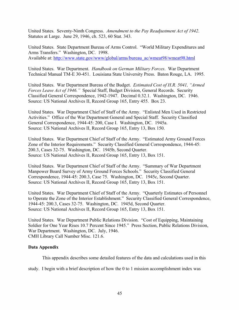
45

United States. Seventy-Ninth Congress. Amendment to the Pay Readjustment Act of 1942.Statutes at Large. June 29, 1946, ch. 523, 60 Stat. 343.

United States. State Department Bureau of Arms Control. “World Military Expenditures and Arms Transfers.” Washington, DC. 1998.Available at: http://www.state.gov/www/global/arms/bureau_ac/wmeat98/wmeat98.html

United States. War Department. Handbook on German Military Forces. War Department Technical Manual TM-E 30-451. Louisiana State University Press. Baton Rouge, LA. 1995.

United States. War Department Bureau of the Budget. Estimated Cost of H.R. 5041, “Armed Forces Leave Act of 1946.” Special Staff, Budget Division, General Records. Security Classified General Correspondence, 1942-1947. Decimal 0.32.1. Washington, DC. 1946. Source: US National Archives II, Record Group 165, Entry 455. Box 23.

United States. War Department Chief of Staff of the Army. “Enlisted Men Used in Restricted Activities.” Office of the War Department General and Special Staff. Security Classified General Correspondence, 1944-45: 200, Case I. Washington, DC. 1945a. Source: US National Archives II, Record Group 165, Entry 13, Box 150.

United States. War Department Chief of Staff of the Army. “Estimated Army Ground Forces Zone of the Interior Requirements.” Security Classified General Correspondence, 1944-45: 200.3, Cases 32-75. Washington, DC. 1945b, Second Quarter. Source: US National Archives II, Record Group 165, Entry 13, Box 151.

United States. War Department Chief of Staff of the Army. “Summary of War Department Manpower Board Survey of Army Ground Forces Schools.” Security Classified General Correspondence, 1944-45: 200.3, Case 75. Washington, DC. 1945c, Second Quarter. Source: US National Archives II, Record Group 165, Entry 13, Box 151.

United States. War Department Chief of Staff of the Army. “Quarterly Estimates of Personnel to Operate the Zone of the Interior Establishment.” Security Classified General Correspondence, 1944-45: 200.3, Cases 32-75. Washington, DC. 1945d, Second Quarter. Source: US National Archives II, Record Group 165, Entry 13, Box 151.

United States. War Department Public Relations Division. “Cost of Equipping, Maintaining Soldier for One Year Rises 10.7 Percent Since 1945.” Press Section, Public Relations Division, War Department. Washington, DC. July, 1946. CMH Library Call Number Misc. 121.6.

Data Appendix

This appendix describes some detailed features of the data and calculations used in this

study. I begin with a brief description of how the 0 to 1 mission accomplishment index was

46

constructed. I then describe the calculations and data sources used for the cost estimates used in

this analysis. The Data Sources section of the Bibliography constitutes an exhaustive list of the

sources used in these calculations. More detailed information on these calculations is available

on request.

A. Construction of Mission Accomplishment Index

Figure A1 shows the worksheet that Dupuy Institute researchers use to judge the

attacker’s mission accomplishment for a given engagement. As the figure shows, each unit is

scored on 3 types of objectives. These include conceptual accomplishment (a general evaluation

of achievement of mission objectives), geographical accomplishment (i.e., miles advanced), and

block hostile mission. Together, these objective-based scores can range from 0 to 6. In addition

to these 3 objective-based measures, the index incorporates general evaluations of the

performance of officers and enlisted men. Together these general evaluations can range from 0

to 4 points. In principle, each side’s mission accomplishment can be evaluated separately and

ranges from 0 to 10. In practice, attacker and defender mission accomplishment are nearly

perfectly negatively correlated. Mission accomplishment ratings do not exceed 8 for either side

for the 164 engagements used in this study. The measure of mission accomplishment used in

this study is (US total score – German total score)/16.

B. Cost Estimates for Infantry and Armored Divisions

One major component of this study is the estimation of dollar costs of operating infantry

and armored divisions. Table A1 shows estimated total costs over the war for infantry and

armored divisions, respectively. The estimated costs are shown for the 1942 Tables of

Organization and Equipment, prior to the reorganization in 1943.94 All dollar figures presented

94 These Tables of Organization and Equipment list the numbers of troops (by rank) and the numbers of specific items allotted to a standard infantry and armored division. As Anderson (2000) mentions, armored divisions

47

in this paper are converted to 2003 dollars using the Consumer Price Index. Some of these

estimates (transportation costs in particular) rely on strong assumptions and should be regarded

as rough approximations. I constructed these estimates using historical data on wages, prices,

and quantities for specific items – together with Army cost studies and budget estimates.

For most major expenditure categories, I find that the costs were very similar for infantry

and armored divisions. The biggest cost differences between the 2 types of divisions were for

equipment and transportation. For an infantry division, equipment costs totaled $230 million in

2003 dollars over the course of the war. For an armored division, equipment costs totaled $2,020

million – nearly 10 times as much. In total, I find that a 1942 organic infantry division cost $1.8

billion. I estimate that a 1942 organic armored division cost more than twice times that, at $4.3

million per engagement.

In Table A1, I estimate the marginal cost of providing infantry and armored divisions to

an overseas combat theater. Table A1 omits many “fixed costs” such as planning, research and

development. While all the Army divisions benefited from these expenditures, these costs do not

have to be paid again when replacing a division. The costs calculated in Table A1 include costs

incurred between the activation of a division and its departure overseas. These costs also include

transportation for the return trip. To compute initial costs for pay and equipment, I combine

quantities data from the Tables of Organization and Equipment with wages and equipment

prices.95 For most of the remaining items, I use raw data and cost studies from US Army

records.

frequently traveled with attached headquarters and supply elements after the 1943 reorganization. Hence, the 1942 Table of Organization and Equipment probably provides a more accurate description of the total cost of supplying tanks to combat. 95 Wage data obtained from US Seventy-Seventh Congress (1942). Equipment prices obtained from US Army Service Forces records.

48

To compute initial (pre-departure) personnel expenditures, I begin with the January 1942

plan for activation of an infantry division.96 This plan specifies the required training and pre-

debarkation employment lengths for all 15,514 troops in an infantry division. I assume that the

sequence of events in activation and training is the same for armored as for infantry divisions. A

division usually began with a cadre of trained, high ranking officers taken from other divisions.

For infantry divisions, this cadre included 172 officers.97 Given the larger numbers of high

ranking officers in an armored division, I assume that the armored officer cadre included 183

officers.98 To compute pay rates for different soldiers, I use the official pay scales approved by

Congress in the Pay Readjustment Act of 1942.99 This document provides the pay scales for

military personnel based on rank, tenure, and special circumstances (e.g., additional skills or

overseas service). I obtain the rank composition of infantry and armored divisions from Hays

(2002, 2000). Because pay depends on tenure, I must assume a level of tenure for each troop.100

The high ranking officers within a division acted as instructors for most of the division’s

training. This training included both basic instruction and field exercises performed at camps

throughout the US. Palmer, Wiley, and Keast (1991) suggest that the typical training period for

96 Source: Palmer, Wiley, and Keast (1991), pp. 433-441. 97 Later in the year, the pre-trained portion of the standard division increased (Palmer, Keats, and Wiley 1991, pp. 436-438). Accounting for such changes would have only a minor effect on my estimated costs. 98 Assuming that the ratio of cadre to other officers was the same as for the infantry division. 99 US Seventy-Seventh Congress (1942). 100 The vast majority of officers and enlisted men who fought in World War II were inducted from civilian life (Palmer, Wiley, and Keast, 1991, pp. 91-92). However, the higher-ranking officers were typically career military. I assume that the core officer cadre had the average tenure levels for their ranks. For other officers and enlisted men, I assume that the troops had zero tenure when they underwent training. After training was complete, I suppose that all these troops had the average tenure levels for their ranks. I assume that this tenure composition was stable over the life of the unit. I estimate average tenure for officers using average pay data from US War Department Bureau of the Budget (1946). Given average pay and the formula relating tenure to pay (from US Seventy-Ninth Congress (1946)), I impute average tenure for each rank. I perform a similar exercise for enlisted men, using average pay data from US Army Office of the Comptroller (1953). Using pay scales from US Defense Department (2004a), I impute average tenure for enlisted men by rank for 1953. I use these 1946 and 1953 average tenure levels to proxy for average tenure in the year of interest. These assumptions about tenure do not affect my estimates but are necessary to obtain wage estimates.

49

a division was 38 weeks.101 I include most of the division’s pre-debarkation wages as personnel

costs, even when the personnel worked as instructors.102 Data from Stanton (1984) indicate that

789 and 803 days passed between activation and departure overseas for armored and infantry

divisions, respectively.103 Hence, the divisions spent a considerable amount of time after training

simply shuffling around and waiting to depart.104 The personnel costs in Table A1 include wages

paid during this idle time.

I obtain the total cost of field exercises from US Bureau of the Budget (1940-1947).105

The average armored and non-armored divisions participated in 1.6 and 2.0 sets of combat

maneuvers, respectively. In total, Army Ground Forces divisions participated in 168 sets of

combat maneuvers.106 I suppose that armored divisions’ maneuvers cost 25% more than for

other types of divisions.107 I then estimate a cost per set of maneuvers by dividing the total cost

across all divisions in proportion to their participation.

All the officers and some of the enlisted men received training prior to the activation of

the division.108 Every officer received both basic enlisted training and some form of basic officer

candidate training. The higher ranking enlisted men received basic enlisted training before 101 Palmer, Wiley, and Keast (1991), pp. 440-441, 481. 102 For training before the division was activated (e.g., basic enlisted training, Officer Candidate School), I include trainee wages in the cost of training. I suppose that basic training for enlisted men and officers occurred prior to activation of the division. Advanced training appears to have frequently taken place after the activation of the division (Palmer, Wiley, and Keats, 1991, pg. 265). Hence, I add wages and allowances for trainees during basic enlisted and officer training and for Command and General Staff training. However, I do not add additional wage costs for the wages of trainees in advanced courses. I suppose that troops hold the rank of Private during basic enlisted training and Private First Class during officer candidate training. I suppose they hold the rank of Second Lieutenant during Command and General Staff Training. For advanced training, I suppose that the trainees hold the same rank as they do during the training of the division. 103 Stanton (1984), pp. 47-182. 104 Brown (1986), pp. 164-167 describes this process in further detail. 105 These estimates exclude the costs of additional military personnel who worked at the training camps. From preliminary investigations, I determined that these additional costs are negligible. 106 Counting each division’s maneuvers separately. Each field exercise typically included multiple divisions. 107 I assume that the armored:infantry cost ratio is the same for maneuvers as for replacement training camps. I describe my estimates of replacement training camp costs later in the appendix. 108 The original officer cadre included officers who had already received training for other purposes – hence, the cost of the division does not include training them. However, the division was responsible for training replacements for the officer cadre in their parent divisions. I include these replacement training costs in the cost of the division.

50

joining the division. Roughly 33% of the officers and roughly 6% of the enlisted men also

received advanced training in some special skill.109 Troops within the division served different

functions (e.g., artillery, infantry, quartermaster), and each troop attended schools particular to

his branch. I obtain data on the breakdown of infantry and armored divisions by branch from

Hays (2004, 2002) and Greenfield, Palmer, and Wiley (1947).110

Next, I determine the lengths and types of training required for each troop. I suppose that

each troop in each division was processed through an induction station and a reception center.

Each of these processes lasted a day or two.111 From early in mobilization until April 1943,

basic enlisted training lasted 13 weeks. Officer candidate school also typically lasted about 13

weeks during this period. By late 1943, both types of schooling had been lengthened to 17

weeks.112 For the purposes of this analysis, I assume that the divisions’ initial troops received

the shorter training. I assume that replacement troops received the longer training. The

specialist courses varied in length. For each branch, I assume that specialist training lasted the

average length for enlisted or officers for that branch. I compute these average lengths using

course lengths and output data from Palmer, Wiley and Keast (1991, pp. 309-319).113 I also

109 I suppose that the training went to the higher ranking officers and enlisted men and to the ranks with “technical” in the title. Both the 33% and 6% figures are rough approximations based on a variety of figures (Palmer, Wiley, and Keats 1991, pp. 249, 266, 279, 308-319). For an enlisted man who learned a special skill, the Army paid an additional allowance. I assume that this bonus coincided with taking the enlisted advanced courses. 110 Greenfield, Palmer, and Wiley (1947, pp. 320-321). Some minor imputation required. 111 War Department Chief of Staff of the Army (1945a). 112 Palmer, Wiley, and Keast (1991, pp. 332, 358, 382-385). 113 For the Officer Candidate School basic training, I also account for the cost of training students who did not graduate. I do this by scaling the course length by the branch-specific graduation rate. I obtain data on graduation rates for the branches of the ground arms (e.g., artillery, armor, infantry) from Keast (1946, pp. 27-34). I obtain data for the overall graduation rate of the service branches (e.g., ordnance, signal, quartermaster) from US Army Service Forces (1954), pg. 224. I assume that the Command and General Staff graduation rate equaled the average graduation rate for basic officer courses in the ground arms. For the basic enlisted training, I assume that the induction centers effectively screened enlisted men, and that the graduation rate was 100%. For advanced courses, I assume that the knowledge (rather than the degree) was relevant for division effectiveness, and I ignore pass rates.

51

suppose that the divisions’ highest ranking officers attended Fort Leavenworth’s 10-week

Command and General Staff course.114

I obtain estimates of the cost per week of officer training from US Army Ground Forces

(1947). This report consists of an itemized accounting of different types of training given to

Chinese officers in 1947. This report includes the estimated costs and lengths for a variety of

courses in ground arms, service branches, and Command and General Staff.115 I also use the

data from Chinese officer course lengths to estimate the length of advanced courses for the

service branches. I assume that the advanced specialist courses cost as much for enlisted men as

for officers. To estimate the cost per week for basic enlisted training, I combine these costs with

data from a few different sources.116

In addition to the initial mobilization strength, each division received replacement troops

when it lost troops due to casualties or other separations. For separations other than casualties, I

include the cost of replacements in the monthly cost of operating a division overseas. I obtain

data on the rate of separations from US Army Service Forces (1954, pp. 200, 206-209). I obtain

data on the rate of casualties (minus returns-to-duty) from US Adjutant General (1953, pg. 5).

114 The course had been abbreviated from the typical 1- to 2-year session for World War II. Partin (1983). 115 I also constructed my own estimates of the average training costs per pupil based on the schools’ non-personnel budgets and the total personnel. My estimates are slightly larger than the Chinese cost estimates, but are generally of the same order of magnitude. According to Palmer, Wiley, and Keats (1991, pg. 274) “requirements for administrative personnel were relatively inelastic, not falling proportionately with the decline in students.” Hence, we should expect the marginal cost of training to fall below the average. 116 I assume that, for each branch, the non-labor cost per pupil was the same for officer training as for enlisted training. I obtain the non-labor costs for the officer candidate schools from US Bureau of the Budget (1940-1947). I then assume that the personnel cost per pupil was proportional to the number of personnel per pupil in each school. I obtain the personnel per pupil for enlisted and officer schools from US War Department Chief of Staff of the Army (1945a through 1945d). I suppose that the labor cost per employee was the same for these schools as for the corresponding branch of officer training. For the service branches, I do not have data on non-labor costs. I assume that the non-labor cost per pupil in the Signal Corps was the same as for Field Artillery. I assume that the non-labor cost per pupil for Ordnance and the Quartermaster Corps are the same as for Infantry. For the Medical Corps, the personnel to student ratio was very similar for basic enlisted and enlisted specialist schools. Consequently, I assume that the cost per trainee week was the same for officers and enlisted men. In general for the service branches, the personnel to student ratios were very similar across officer and enlisted schools. For Military Police and Engineer Corps, I do not observe personnel to student ratios for both officer and enlisted courses. For these 2 branches, I assume that the cost per trainee week was the same for enlisted men as for officers.

52

Using these data, I estimate the monthly rates of non-casualty separations for officers and

enlisted men. Within each enlisted/officer and branch combination, I assume that the fraction

taking specialist courses was the same as with the original division. However, replacements

generally did not receive divisional training or participate in maneuvers. For casualty

replacements, I obtain the fatality rate per branch from a handful of sources.117 I do not include

the cost of replacing casualties in the monthly costs of the divisions. Instead, I estimate this cost

separately and report it separately in the text.

I obtain initial quantities requirements for major divisional equipment for infantry and

armored divisions from Hays (2004, 2002).118 The unit prices I use come from US Army

Services of Supply (1942a, 1942b) and US Army Service Forces (1942a, 1942b, 1943a, 1943b,

1943c, 1944a).119 I adjust these prices for using branch-specific monthly procurement price

indices from Crawford and Cook (1953), pg. 82. I estimate the maintenance and replacement

requirements for different items using depreciation rates from US Army Service Forces (1943d,

1944b, 1944c). These depreciation rates take into account tank losses both in and out of

combat.120 In many cases, Army Service Forces estimated separate depreciation rates for

different theaters. When separate depreciation rates were available for the Mediterranean and

European Theaters of Operations, I used an average of the 2 rates. When this was not possible, I

used depreciation rates for the overall Western Front or for the entire overseas army.

117 US Adjutant General (1953), pg. 5. Palmer, Wiley, and Keast (1991), pg. 49. US Army Service Forces (1954), pg. 123. Some branches aggregated. Some minor imputation required. Infantry accounted for the vast majority of casualty replacements. I suppose that the ratio of enlisted to officer casualties was constant across the different ground arms and service branches. 118 I use the 1942 Tables of Organization and Equipment for both infantry and armored divisions. 119 And one airplane price from United States Army Air Forces (1945). 120 I assume constant monthly depreciation rates, as US Army Service Forces did when determining replacement requirements. These depreciation rates take into account tank losses from combat. Simply using tank loss rates from the engagement data would fail to account for tank losses out of combat. Moreover, the engagement-level tank loss data do not specify the degree of damage or reparability. These constant monthly depreciation rates appear to be the most accurate way to account for tank losses.

53

Maintenance and loss data from overseas were limited, and these estimated depreciation rates are

at best very rough approximations. In a small handful of cases, the price or depreciation rate for

a specific item was not available. In these cases, I used the prices or depreciation rates for

similar items. For the 38 weeks of division training, I suppose that equipment depreciated at the

reported rates for the Continental US. I treat this depreciation as a cost of training. For the

remaining idle time pre-debarkation, I suppose that equipment did not depreciate.

For food, clothing, gasoline, and ammunition costs, I rely on a handful of historical US

Army cost studies. For a single troop’s food requirements, I use estimates from US War

Department Public Relations Division (1946). For clothing and additional equipment, I use

estimates from US Army Office of the Quartermaster General (1944).121 I then multiply both per

troop estimates by the number of men in each type of division. I obtain monthly overseas

ammunition cost estimates for a 1942 armored and infantry division from US Army Services of

Supply (1943, pg 30). I obtain monthly overseas gasoline requirements for a 1942 armored and

infantry division from US Army Service Forces (1943a).122 I then compute costs for these

gasoline requirements using the 1942 price for a gallon of gasoline from US Bureau of Labor

Statistics (2004b).

Calculating the costs of a division’s transportation is a complicated issue. I employ a

number of strong assumptions to arrive at a very rough estimate for the cost of a division’s

transportation. First, I obtain estimates of the US Army’s total travel- and transportation-related

expenditure from US Bureau of the Budget (1940 to 1947).123 Next, I obtain data on the total

121 These Quartermaster General estimates include both initial costs and monthly maintenance costs. I also add 25% of the initial costs for reserve requirements, as the study suggests. These totals include “additional equipment” such as canteens, flashlights, etc. I add these costs to the “Equipment” category in Table A1. 122 These studies do not report monthly ammunition or gasoline requirements for units still in the US. For the 38-week training period, I suppose that gasoline and ammunition usage was proportional to capital depreciation. 123 Travel appears as a separate item in the War Department’s budget. For earlier years, transportation appears in the Quartermaster section of the budget, and for later years, the Transportation Corps has its own section. In both cases,

54

number of passengers and tons moved overseas by the US Army.124 I divide the Transportation

Corps budget by the number of tons to obtain the total shipping cost associated with each ton

moved overseas. I assume that transportation cost the same per ton and per passenger for the

Pacific and Western Fronts. In addition to sending shipments overseas, the US Army used

considerable resources transporting troops and equipment across the US and Europe. I assume

that the Transportation Corps had zero fixed costs and that the intra-continental transport costs

were the same for each ton. Given all these assumptions, I arrive at a cost estimate of $800 per

ton. I divide the total Army travel expenditure by the number of troops shipped overseas to

obtain the total travel cost for each troop. Hence, I assume that intra-continental travel costs

were the same for each troop. I arrive at a total travel cost per troop shipped of $3,300.

I obtain the weight (in tons) of an infantry and armored division’s equipment from US

Army Service Forces (1943a). I assume that initial shipping costs include the cost of a 2-way

trip for each troop and each ton of material. However, for monthly maintenance and troop

replacements, I assume 1-way trips. I assume maintenance shipments had the same weight per

dollar of expenditure as the initial shipments did. In addition to regular purchases, Army supply

plans included a 4.5-month store of reserves.125 Hence, I add 4.5 months of equipment, gasoline,

and ammunition to the initial cost of each division type. I allow for 2% shipping losses for all

equipment, as suggested in Denson and Wood (1943), pg. 21.126

these budgets only report non-labor expenditure. To compute Transportation Corps labor costs, I obtain the branch strength for various years from Greenfield, Palmer, and Wiley (1947), pg. 203. I estimate the cost per employee by dividing the “Pay of the Army” section of the budget by the US Army’s total military personnel. Some minor amounts of imputation required. 124 These data come from US Army Service Forces (1953), pp. 116, 123. 125 Denson and Wood (1943), pg. 21. A preliminary examination of storage costs revealed that these were negligible. Supplies ran very low near the end of the war. As Anderson (2000) describes, to supply units in the field, some divisions were stripped of their equipment as soon as they arrived overseas. Hence, the true amounts of reserves maintained overseas may have fell considerably lower than this 4.5 months figure. 126 In other words, all equipment costs are divided by 0.98 to allow for shipping losses.

55

Putting these figures together, I estimate that a 1942 organic infantry division cost $812

million fixed plus $48.6 million per month abroad. I estimate that a 1942 organic armored

division cost $1,910 million fixed plus $132 million per month abroad. The average US infantry

and armored divisions sent to the Western Front spent 19.4 and 18.2 months abroad,

respectively.127 The figures in Table A1 assume 1942 organic infantry and armored divisions

that spent 19.4 and 18.2 months abroad, respectively.

To determine the cost of a single troop, I to each troop his share of the total expenditure

of a 1942 organic infantry division. That is, I divide $812 million fixed plus $48.6

million/month by 15,514, the number of troops in a 1942 organic infantry division. This cost

comes to $52,000 fixed plus $3,100 per month abroad. To determine the cost per tank, I subtract

troop-related expenditures (i.e., 14,620 times the cost per troop) from the armored division’s

cost. This figure gives the total equipment, ammunition, gasoline, transportation, and other costs

that armored divisions paid that equally-sized infantry divisions did not. I then divide by 390,

the number of tanks in a standard armored division.128 That is, I attribute to each tank its share

of supporting equipment and other armored division expenditures.129 This cost comes to $2.9

million fixed plus $221,000 per month abroad. I assume that the costs per troop and tank are

constant across divisions.

Next, I take these fixed and monthly costs per troop and tank, and I apply them to the

infantry and armored divisions in the 164-engagement database. For each observation, I

multiply the costs per troop and tank by the numbers of troops and tanks, respectively. I assume

that each unit in the data spent 19.4 months abroad, and that the each armored division spent 18.2

127 Data source for months abroad: Stanton (1984), pp. 47-182. 128 The division’s equipment also included other armored vehicles such as tank destroyers and armored cars. However, in the engagement data, only the tanks are counted. Hence, for the purposes of this exercise, I only count the tanks. 129 This supporting equipment includes other armored vehicles such as armored cars and tank destroyers.

56

months abroad. Given the costs per troop and tank and the total months abroad, I then compute

the total wartime cost for each division. Next, I divide these total costs by the total number of

combat days fought by each type of division. Combat days are not formally defined, but were

reported by individual divisions. These data appear in Ruppenthal (1959, pp. 282-283) and US

Army Historical Services Division (1962).130 For the cases when data exist, combat days

averaged 202 for infantry divisions and 118 for armored divisions. Hence, for each infantry

division, I divide its total costs by 202. For each armored division, I divide its total costs by

118.131 Averages for these daily cost estimates appear in Table 2 and are $14.4 million for

infantry and $29.7 million for armored. To obtain per day costs for infantry and armored

divisions, I solve a system of 2 linear equations:

(A1) $14.4 million = 19,200* miW + 110* m

iR , and

(A2) $29.7 million = 12,300* miW + 267* m

iR ,

where 19,200 and 12,300 are the average numbers of troops for infantry and armored divisions in

the data. And 110 and 267 are the average numbers of tanks for infantry and armored divisions

in the data. Solving this system of equations, I obtain costs of $751 per troop per combat day

and $65,300 per tank per combat day.

To calculate the costs in Table 1, I estimate the numbers of troops and tanks in the

average organic infantry and armored division. Of the 47 infantry divisions that went abroad,

roughly 14% of the time was spent under the 1942 structure. Of the 16 armored divisions that

130 Data for combat days are missing for the US 1st Armored and 85th Infantry Divisions. 131 In principle, given the US Army Adjutant General (1953) casualties data and the engagement-level data, it should be possible to estimate combat days. However, I obtain wide variance in estimated days depending on the measure of casualties used. Using data on total casualties, I find that infantry divisions fought 12% more days of combat. Using data on killed in action, I find that infantry divisions fought 78% more days of combat. The killed in action data are generally more variable. In a private conversation, however, Chris Lawrence of The Dupuy Institute has suggested that the killed in action data are more reliable. The definition of wounded in action tended to change depending on the level of combat intensity. Wounds were generally recognized and treated more often during low-intensity conflicts.

57

went abroad, roughly 12% of the time was spent under the 1942 structure. I construct a weighted

average of 0.14 times a 1942 infantry division’s troops plus 0.86 times a 1943 infantry division’s

troops.132 This figure gives the average number of troops in an organic infantry division. I

construct this same type of weighted average for the troops and tanks for an infantry and armored

division. The average numbers of troops and tanks in each division type appear in Table 1. I

find that the average organic infantry division included 14,400 troops and 66 tanks. I find that

the average organic armored division included 11,500 troops and 281 tanks. I assume that the

average infantry division spent 19.4 months abroad and that the average armored division spent

18.2 months abroad. I then use the fixed and monthly per troop and per tank costs described

above to calculate the total wartime costs. These totals come to $2.1 billion for an organic

infantry division and $3.1 billion for an organic armored division.

132 Data Sources: Greenfield, Palmer, and Wiley (1947), pg. 333; Wilson (1997), pg. 187; Stanton (1984), pp. 47-51.

Infantry Armored Difference

Troops 14,400 11,500 2,900

Tanks 66 281 -215

Battle-RelatedDeaths 2,077 825 1,252

Battle-RelatedNonfatal Injuries 6,972 2,741 4,231

Estimated Dollar Cost(in 2003 Dollars) $2.1 billion $3.1 billion -$1.0 billion

Table 1: Dollar Cost and Battle Casualties Over the EntireWar for the Average US Infantry and Armored Division

Notes: Estimated dollar costs, deaths, and injuries all represent totals for the entire war. Death and injury figures represent averages taken across all 47 US infantry and 16 US armored divisions that fought on the Western Front. Deaths include soldiers killed in action, dead from battle-related injuries, dead in captivity, and missing and presumed dead. Troops and tanks are taken from the US Army's defintions of infantry and armored divisions, from US Army Table of Organization and Equipment. These definitions changed in 1943. The troop and tank figures presented here are weighted averages that take into account the length of time that each division spent under 1942 organization and the 1943 organization. Source for deaths and injuries: US Army Adjutant General (1953), pp. 84-88. Dollar costs estimated from various archival sources.Additional sources and calculations described in the Data Appendix.

t-Statistic forEquality of

Variable Infantry Armored Sample Means

US Mission Accomplishment 0.56 0.58 0.5US Killed in Action per Day 19.3 15.3 -0.6German Killed in Action per Day 21.5 51.6 5.4**US Wounded in Action per Day 106 81.3 -0.7German Wounded in Action per Day 63.1 178 7.2**Estimated Dollar Cost per Day (in 2003 dollars) $14.4 mil $29.7 mil 5.0**

US Troops 19,200 16,300 -2.4**German Troops 12,300 9,800 -2.4**US Tanks 110 267 3.7**German Tanks 38.4 33.6 -0.5US Aerial Sorties/Day 17.0 11.6 -1.0German Aerial Sorties/Day 4.8 0.0 -3.3**

US is Attacker 0.88 0.90 0.4US Troops per Meter of Front Width 2.3 2.1 -0.6Duration of Engagement 2.0 1.7 -0.8Mountain or River Battle 0.21 0.05 -1.8*Rugged Terrain 0.47 0.50 0.2Wet or Rainy 0.37 0.35 -0.3Temperate Climate 0.45 0.25 -0.9Wooded or Mixed Vegetation 0.86 1.00 2.0*Urban or Conurban 0.08 0.00 -1.5

Index (0 to 1) for US Advantage in:Leadership 0.57 0.51 -1.9*Training & Force Quality 0.61 0.61 0.0Intelligence & Planning 0.51 0.52 0.2Logistics & Reserves 0.54 0.52 -0.7Morale 0.58 0.58 -0.2Surprise 0.52 0.55 0.9Defender Fortifications 0.36 0.28 -2.0*

Observations 144 20 164Unique Divisions 16 4 20

Table 2: Sample Means for Infantry and Armored Divisions from Engagement-Level Data

Notes: Each observation is a single, 1- to 12-day engagement between US and German forces. All data are for land battles fought on the Western Front in World War II. Killed in action and wounded in action are imputed as a constant fraction of casualties for roughly 38% of the data. T-tests assume robust standard errors clustered by US division. Additional details in the Data Appendix. Sources: Land Warfare Database and The Dupuy Institute's Division-Level Engagement Database .** denotes 5% significance. * denotes 10% significance.

(1) (2) (3) (4) (5) (6)

US Troops/10,000 0.033 0.068 0.100 0.103 0.071 0.083(0.024) (0.031)* (0.036)** (0.038)** (0.028)** (0.028)**

US Tanks/100 0.017 0.010 0.017 0.014 0.014 0.020(0.012) (0.011) (0.014) (0.017) (0.014) (0.013)

Includes Controls For:Enemy Inputs Yes Yes Yes Yes YesAerial Sorties Yes Yes Yes YesTerrain and Weather Yes Yes Yes YesLocation X Year Interactions Yes YesHuman Factors Yes Yes

R20.08 0.11 0.29 0.33 0.59 0.62

Table 3: First-Stage Regression: Effects of Troops and Tanks on Mission Accomplishment

Dependent Variable is a 0 to 1 Index of US Mission Accomplishment

Notes: See notes to Table 2. Each column shows coefficients from a separate linear regression. Sample includes 164 observations.The dependent variable is a continuous index from 0 to 1 representing historians' subjective judgments about how successful theUS force was. Each column shows coefficients from a separate regression. Robust standard errors, clustered by US division, areshown in parentheses. Enemy input controls include German troops and German tanks. Aerial sorties include close combat sortiesper day (bombers and fighters together), measured separately for US and German forces. Terrain and weather controls include dummies for European/Mediterranean Theater, mountain battle, river battle, rolling terrain, rugged terrain, urban, conurban, wooded vegetation, mixed vegetation, wet, light rain, heavy rain, and cold. Location X Year interactions include year dummies interacted with dummies for the country in which the battle took place (Belgium, France, Germany, Italy, Luxembourg, or Tunisia)."Human factor" controls include attacker/defender status interacted with dummies for fortified defense and prepared defense, and 0 to 1 indices for US advantage in each of leadership, intelligence, planning, reserves, training, force quality, morale, air superiorityand defensive fortifications. Each specification includes a constant term, a dummy for attacker/defender status, and a dummy forwhether the observation's killed in action figures are imputed. Additional details in the text.

(1) (2) (3) (4) (5) (6)

US Troops/10,000 6.9 7.6 12.4 12.0 11.1 14.1(4.8) (5.3) (3.9)** (4.0)** (4.4)** (3.6)**

US Tanks/100 0.3 0.1 -1.0 -0.9 -0.3 -0.6(2.8) (2.7) (3.7) (3.6) (2.1) (2.0)

Includes Controls For:Enemy Inputs Yes Yes Yes Yes YesAerial Sorties Yes Yes Yes YesTerrain and Weather Yes Yes Yes YesLocation X Year Yes YesHuman Factors Yes Yes

R20.09 0.09 0.27 0.29 0.49 0.52

Table 4: First-Stage Regression: Effects of Troops and Tanks on US Killed in Action

Dependent Variable is Number of US Killed in Action per Day of Combat

Notes: See notes to Tables 2 and 3. Data on US Killed in Action are missing 62 of these 164 observations. In those cases, Killed in Action is imputed as 0.12 times US Casualties (where casualties include killed, wounded, and missing in action).

(1) (2) (3) (4) (5) (6)

US Troops/10,000 40.8 68.0 65.5 104 -1.23 -2.42(29.3) (22.4)** (53.2) (38.4)** (2.12) (2.07)

US Tanks/100 -0.1 -6.4 4.4 4.0 3.72 4.68(14.3) (11.5) (23.2) (17.0) (0.74)** (1.30)**

Includes Controls For:Enemy Inputs Yes Yes Yes Yes Yes YesAerial Sorties Yes Yes YesTerrain and Weather Yes Yes YesLocation X Year Yes Yes YesHuman Factors Yes Yes Yes

R2 0.07 0.46 0.06 0.58 0.34 0.56Observations 164 164 164 164 126 126

Table 5: Effects of Troops and Tanks on Other Outcomes

Wounded in Action per Day Tank Losses per DayDependent Variable is US Dependent Variable is USDependent Variable is

US Casualties per Day

Notes: See notes to Tables 2 and 3. Casualties include soldiers killed, wounded, captured, or missing.

(1) (2) (3)

US Fatalities per Day $41,000 $25,000 $26,000(38,000) (38,000) (24,000)

US Mission Accomplishment $11.3 mil $10.5 mil $12.3 mil(4.0 mil)** (3.0 mil)** (3.9 mil)**

Includes Controls For:Enemy Inputs Yes Yes YesAerial Sorties Yes YesTerrain and Weather Yes YesLocation X Year Interactions YesHuman Factors Yes

R20.15 0.56 0.70

Table 6: Cost per Life Saved, OLS Estimates

Dependent Variable is Estimated US Dollar Expenditure per Combat Day (in 2003 Dollars)

Notes: See notes to Tables 2 and 3. The dependent variable is constructed as $751*(US Troops) + $65,300*(US Tanks). These per troop and per tank costs are estimated from a variety of sources, as described in the Data Appendix. The first regressor is US Battle Fatalities per Combat Day. The coefficient on this regressor is -1 times the estimated willingness-to-pay of the US government to reduce fatalities. Total US Battle Fatalities were not measured by engagement, however, US Battle-Related Fatalities were 1.18 times US Killed in Action. This regressor is constructed as 1.18*US Killed in Action per Combat Day. The second regressor is acontinuous index from 0 to 1 representing historians' subjective judgments about how successful the US force was. The coefficient on this regressor is the estimated willingness-to-pay of the US government to increase mission accomplishment from 0 to 1. Additional details in the text.

(1) (2) (3) (4) (5) (6)

US Fatalities per Day -$0.7 mil -$4.6 mil -$1.4 mil -$1.9 mil -$1.7 mil -$1.0 mil(1.8 mil) (14.9 mil) (2.2 mil) (3.5 mil) (3.0 mil) (1.1 mil)

[95% Confidence Interval] [-244, 1.6] [-433, -1.6]** [-462, -0.1]** [-158, -0.2]** [-367, -0.2]** [-778, 0.8]

US Mission Accomplishment $411 mil $725 mil $284 mil $330 mil $428 mil $297 mil(308 mil) (1,670 mil) (284 mil) (413 mil) (513 mil) (198 mil)

Includes Controls For:Enemy Inputs Yes Yes Yes Yes YesAerial Sorties Yes Yes Yes YesTerrain and Weather Yes Yes Yes YesLocation X Year Interactions Yes YesHuman Factors Yes Yes

R2-47.9 -274 -27.5 -39.3 -28.5 -10.5

Table 7: Second-Stage Regression: Cost per Life Saved, Instrumental Variables Estimates

Dependent Variable is Estimated US Dollar Expenditure per Combat Day (in 2003 Dollars)

Endogenous Regressors: US Fatalities per Day and US Mission AccomplishmentExcluded Instruments: US Troops and US Tanks

Notes: See notes to Tables 2 and 3. Bias-corrected 95% confidence interval estimated using a bootstrap with 1,000 repetitions ofsample size N, clustered by US division. Confidence interval expressed in millions. The coefficient on US Battle Fatalities perDay is -1 times the estimated willingness-to-pay of the US government to reduce fatalities.

** indicates 95% confidence interval does not include zero.

US Cost perUS Tanks per Life Saved1,000 Troops (IV Estimate) Notes

US is Attacker, N=144 6.9 -$0.1 milUS is Defender, N=20 7.0 $2.3 mil

US has Air Support, N=59 7.0 -$0.7 milUS has No Air Support, N=105 6.9 $0.8 mil

German Troops Low, N=82 7.5 $1.2 mil High, N=82 6.4 $12.5 mil

Armored Division, N=20 16.5 -$0.4 milInfantry Division, N=144 5.6 $12.2 mil

Leadership US Advantage, N=50 6.8 $1.8 mil US & Germans Equal, N=114 7.0 $0.5 mil

Mountain or River, N=31 4.7 $0.5 milNo Mountain/River, N=133 7.5 $1.4 mil

Early, N=55 4.5 $0.2 milMiddle, N=55 7.9 -$1.8 milLate, N=54 8.5 $0.1 mil

Table 8: Tank Intensity and Estimated Cost per Life Saved for Subsets of the Data

Panel A: Shadow Prices Common Across Subsets

Panel B: Shadow Prices are Different Across Subsets

Notes: See notes to Table 7. In this table, I estimate the dollar cost per life saved for various subsets of the data. Cost per life saved estimated in the same way as in Table 7. Regressions all control for enemy inputs, aerial sorties, and terrain and weather, as in Column (3) of Table 7.

Mountains, and rivers are additional, unmeasured costs of tank use. For the total (measured + unmeasured) cost to be the same across the two cases, the measured cost per life saved should be lower in mountains, and rivers. The cost of tanks lowered over the war due to accumulated production and learning. Hence, the measured cost should have increased over time.

Attacker/defender status, leadership quality, division type, and the presence of air support may affect the usefulness of tanks. However, they do not affect the costs of supplying tanks. If the US Army were perfectly efficient, then the cost per life saved would be equal across the 2 subsets in each case.

(1) (2) (3)

Benchmark Model (N = 164) $4.6 mil $1.9 mil $1.0 mil

Including Additional Administrative Costs $3.7 mil $1.1 mil $0.6 milUsing Alternative (Army Service Forces) Estimates for Tank Costs $3.5 mil $1.1 mil $0.8 mil

Ignoring Light Tanks $0.3 mil $0.3 mil $0.2 milAssuming Wounds 1/10 as Costly as Fatalities $2.9 mil $0.9 mil $0.8 mil

Including Troop-Tank Interactions $0.9 mil $0.5 mil $0.5 milLog-Log Model, N=160 $10.0 mil $4.1 mil $2.9 milLog-Log Model with Troop-Tank Interactions, N=160 $3.6 mil $2.7 mil $1.6 milSquare Root Model $2.2 mil $2.2 mil $1.8 mil

Including Regiment-Level Engagements, N=199 $9.7 mil $1.4 mil $1.1 milIncluding Corps-Level Engagements, N=204 $0.4 mil -$1.1 mil -$1.8 milIncluding All Available Data, N=230 $0.0 mil -$1.1 mil -$2.1 mil

Excluding US 1st Armored Division, N=162 $1.4 mil $0.6 mil $1.0 milExcluding Imputed Obs from Killed in Action Regression, N=164, 102 $0.8 mil $0.8 mil $4.6 milExcluding Imputed Obs from Both Regressions, N=102 $0.3 mil $1.3 mil -$2.4 mil

Using Win-Lose-Draw for Mission Accomplishment -$5.8 mil $2.5 mil $0.5 milUsing Miles Advanced per Day for Mission Accomplishment -$0.5 mil -$0.9 mil -$0.3 mil

Excluding Observations with Attacker Success:Lower Than 0.20, N=157 $127 mil $3.1 mil $1.2 milLower Than 0.40, N=137 -$8.7 mil $12.1 mil $1.3 mil

Includes Controls For:Enemy Inputs Yes Yes YesAerial Sorties Yes YesTerrain and Weather Yes YesLocation X Year YesHuman Factors Yes

Cost per Life Saved (IV Estimate)(in 2003 Dollars)

Table 9: Sensitivity Analysis — Cost per Life Saved Using Alternative Models

Specification

Notes: See notes to Table 7. Each number in this table represents a cost per life saved estimate from a slightly different model. In each case, I calculate the cost per life saved in the same way as in Table 7.

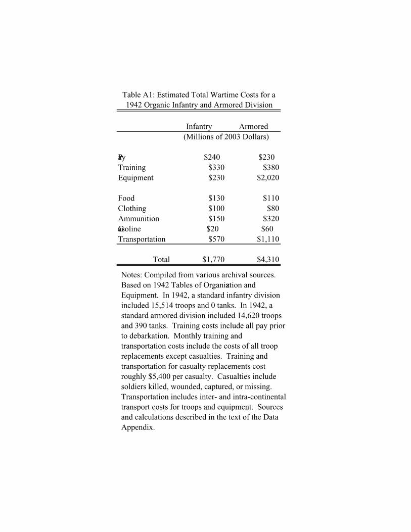
Infantry Armored

Pay $240 $230Training $330 $380Equipment $230 $2,020

Food $130 $110Clothing $100 $80Ammunition $150 $320Gasoline $20 $60Transportation $570 $1,110

Total $1,770 $4,310

(Millions of 2003 Dollars)

Table A1: Estimated Total Wartime Costs for a1942 Organic Infantry and Armored Division

Notes: Compiled from various archival sources.Based on 1942 Tables of Organization and Equipment. In 1942, a standard infantry division included 15,514 troops and 0 tanks. In 1942, a standard armored division included 14,620 troops and 390 tanks. Training costs include all pay prior to debarkation. Monthly training and transportation costs include the costs of all troop replacements except casualties. Training and transportation for casualty replacements cost roughly $5,400 per casualty. Casualties include soldiers killed, wounded, captured, or missing.Transportation includes inter- and intra-continental transport costs for troops and equipment. Sources and calculations described in the text of the Data Appendix.

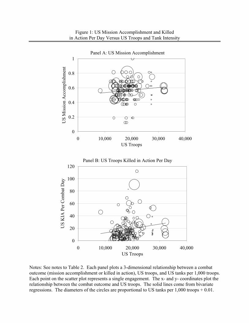
Figure 1: US Mission Accomplishment and Killed in Action Per Day Versus US Troops and Tank Intensity

Panel A: US Mission Accomplishment

0

0.2

0.4

0.6

0.8

1

0 10,000 20,000 30,000 40,000US Troops

US

Mis

sion

Acc

ompl

ishm

ent

Panel B: US Troops Killed in Action Per Day

0

20

40

60

80

100

120

0 10,000 20,000 30,000 40,000US Troops

US

KIA

Per

Com

bat D

ay

Notes: See notes to Table 2. Each panel plots a 3-dimensional relationship between a combat outcome (mission accomplishment or killed in action), US troops, and US tanks per 1,000 troops. Each point on the scatter plot represents a single engagement. The x- and y- coordinates plot the relationship between the combat outcome and US troops. The solid lines come from bivariate regressions. The diameters of the circles are proportional to US tanks per 1,000 troops + 0.01.

Figure 2: Graphical Illustration of Mission Accomplishment Isoquants

Panel A: Production Isoquants and Isocost Sets for Fatality-Neutral and Fatality-Averse Armies

Panel B: Variation in L and K Driven by Unobserved Changes in Shadow Prices

Figure A1: Mission Accomplishment Worksheet for Dupuy Institute Databases

Engagement name:____________________________

Engagement date:_____________________________

Assessment date: ____________ Assessor's Initials: _______

Attacker Defender

Unit:______________________ Unit: _____________________

Conceptual Accomplishment: 0 Conceptual Accomplishment: 0 1 1 2 2

Geographical Accomplishment: 0 Geographical Accomplishment: 0 1 1 2 2

Block Hostile Missions: 0 Block Hostile Mission: 0 1 1 2 2

Command & Staff Performance: 0 Command & Staff Performance: 0 1 1 2 2

Troop Performance: 0 Troop Performance: 0 1 1 2 2

Bonus or Penalty: Bonus or Penalty: Explain: Explain:

Total Score: _______ Total Score: _______

Notes: The 0-1 index of US Mission Accomplishment used in this study is calculated as the (US Total Score – German Total Score)/16. Source: The Dupuy Institute (2001a).