Department of Economics and Finance

Working Paper No. 09-40

http://www.brunel.ac.uk/about/acad/sss/depts/economics

Econ

omic

s an

d Fi

nanc

e W

orki

ng P

aper

Ser

ies

Ahmed Alzahrani and Len Skerratt

How Markets React to Earnings Announcements in the Absence of Analysts and Institutions Evidence from the Saudi Market

November 2009

1

“How Markets React to Earnings Announcements in the Absence of Analysts and

Institutions: Evidence from the Saudi market”

Ahmed Alzahrani and Len Skerratt

Abstract:

How stock markets react to news is an established area of research. We examine the behaviour

of the Saudi Stock market in response to earnings announcements where there are no analysts’

forecasts, with the aim of examining the efficiency of the market. The SSM seems to underreact

to positive news for the first five days and then reactions tend to strengthen in the following

weeks, indicating the presence of a post–earnings announcement drift, or PEAD. At the same

time, the SSM overreacts to negative news in the first five days and then reverses its direction

and reports an upward post-earnings announcement drift. The individually dominated market

combined with the absence of analysts’ forecasts is the main explanation for this underreaction

to positive news and overreaction to negative news.

JEL Codes:G14, G15, M40

Keywords: Post-Earnings Announcement Drift, Market Efficiency, Analysts’ forecasts, Saudi Stock

Market, Over and Under-reaction.

2

1 Introduction

This paper makes several contributions. First, we test the existence of post-earnings

announcement drift (PEAD) in a comprehensive sample in a less developed market. Second, we

provide a perspective on the way in which a market reacts to earnings announcements in the

absence of analysts’ forecasts. We test for PEAD effects not only in general, but also across

industries on the stocks listed on the Saudi stock exchange. Third, the Saudi Stock Market

(hereafter, SSM) is dominated by retail investors, which provides a perfect setting for studying

investor behaviour and reaction to informational events. Fourth, the SSM has certain

characteristics which distinguish it from many developed and emerging markets (e.g., high

government ownership, larger market capitalisation and company size, highly active trading,

lack of options and short selling and finally a market that is dominated by individuals). It is

interesting to study the effect of these unique aspects of the SSM on stock trading and returns,

especially in regard to earnings announcements.

Many stock markets in developing countries such as Saudi Arabia have no or a few

financial analysts who – regularly – follow stocks and issue forecasts and recommendations.

There is supporting evidence of high information asymmetry in developing stock markets which

can be attributed to many other factors, including information intermediaries and corporate

disclosure practice. Any attempt to measure market reaction to news in the SSM is essentially

measuring retail investor’s reaction because they dominate the market. We aim in this study to

examine how the absence of analysts can impact the behaviour of the market. If the there is no

price drift in the market, we can infer that PEAD is caused by analysts herding and bias.

However, if the price drift is larger in magnitude, we can safely infer that analysts are important

agents for the price impounding process to take places and for the market efficiency in general.

We study, indirectly, the impact of different market characteristics (the SSM being, for

example, a market less followed by analysts, with inactive institutional investors and where

short sales are not allowed) on market behaviour in regard to earnings news. We believe that the

SSM is distinct from other developed markets in that it lacks active presence of analysts who

are important information intermediaries in the market.

2 Literature Review

How investors perceive, interpret and react to news has been an active area of research since the

seminal work of Ball and Brown (1968). They empirically investigated the association between

accounting earnings as the core information in financial statement and stock returns in order to

assess the usefulness of accounting information. They were the first to report a drift in the stock

returns after earnings announcements, a phenomenon which was later given the name of the

Post-Earnings Announcement Drift (PEAD). Since then, many researchers have confirmed the

robustness of PEAD using different techniques and different data (e.g., Foster et al., 1984;

Bernard and Thomas, 1998, 1990; Ball and Bartov, 1996; and Chordia and Shivakumar, 2005).

3

Capital markets research findings suggest that earnings announcements contain information

which is believed to alter investors’ opinion about the value of stocks through the process of

impounding information on prices.

PEAD is the continuous upward (downward) drift in prices after positive (negative)

news. The price drift is the result of a persistent underreaction to earnings news. It suggests that

the market underreacts to information on earnings announcements and hence that future returns

are somewhat predictable. PEAD is considered one of the most robust stock market anomalies to

be considered in the financial literature. The Efficient Market Hypothesis (EMH) states that

prices should fully and instantaneously reflect all publicly available information.1 Hence, an

efficient market should incorporate all information (factual or predicted) into prices in a quick

and unbiased way. A price drift in general indicates that the market fails to translate the

information into prices. For this reason, many researchers consider the price drift to be a serious

empirical challenge to EMH.

While most of the PEAD studies concentrated first on US markets and data, more recent

studies have expanded the coverage to other European and emerging markets worldwide.

However, the mainstream evidence comes from US data and other stock markets have attracted

little research .Naturally, the UK market has become the second most studied market in terms of

price drift but beyond this only a few other European or Asian markets have been the subject of

studies, a mere handful, and other markets in the Middle East and North Africa have hardly been

studied at all.

Why stock prices drift after the earnings announcement

While the PEAD is well documented in the literature, the reasons for the persistent

underreaction to earnings announcements are not well understood. This phenomenon can be

explained with a number of hypotheses, but two competing hypotheses and explanations

dominate the debate. The first is the rational explanation and the second comes from the

behavioural school which suggests that investors are irrational. Advocates for the rational and

efficient market claim that PEAD can be explained by the inaccuracy of the tools used by

researchers to detect the price drift, an inaccuracy which may stem from returns

mismeasurement, risk mismeasurement or methodological biases in general. They also attribute

importance to such causes for the drift as the rational risk premium and transaction cost. This

rational explanation views the price drift anomaly as a compensation for risk associated with

shocks in the earning news (See, for example, Foster et al, 1984; Dyckman and Morse, 1986;

Garfinkel and Sokobin, 2006).

The difficulty in explaining the PEAD by an argument consistent with market efficiency has

motivated the behavioural explanations. Behavioural finance generally argues that irrationality

in the form of one or more cognitive biases has led to observed patterns of abnormal returns.

Because of shared human attributes, such as overconfidence, greed or fear, people make errors

of judgment, which are a deviation from the assumption of rational expectations in economics

and the Efficient Market Hypothesis. Findings suggest that PEAD is related to investors’

4

underraction or overreaction to earning news (see, for example, DeBondt and Thaler, 1985;

Bernard and Thomas, 1998; and Daniel et al., 1998). A common explanation for this

phenomenon is that investors underreact to earnings news and they also fail to recognise the

serial autocorrelation patterns in quarterly earnings (Bernard and Thomas, 1990; Ball and

Bartov, 1996).

Another line of research, more relevant to our paper, is aimed to distinguish between individual

trading and institutional trading. Several studies suggest that institutional trading is more

sophisticated than individual trading and accordingly, individual trading may be more

responsible for the PEAD than institutional trading is (see, for instance, De Franco et al, 2007).

Hirshleifer et al. (2008) call it the individual trading hypothesis. Bhattacharya (2001) and

Battalio and Mendenhall (2005) provide evidence consistent with the conjecture that individuals

cause the PEAD.

The magnitude of the drift may differ for good and bad news. Management plays an

important part in explaining overreaction and underreaction to news. When there is good news,

it is announced immediately. It benefits the management to announce all positive news.

However, when there is negative news, management tends to announce it at some point in time

but maybe to delay it (see, for example, Hong et al., 2000)

Market Expectation proxy (the Earning Surprise)

Kothari (2001) emphasises that the degree of return-earnings association is crucially affected by

the accuracy of the proxy set by the researcher for the unexpected earnings. It is common for

most market reaction studies to measure standard unexpected earnings (SUE), which are defined

as actual earnings minus expected earnings standardised by earning variance. Unexpected

earning is considered the explanatory variable in the regression analysis which enables us to

understand why the market reacts in such a way.

Many measures have served as proxies for unexpected earnings or the surprise component of

earnings, the two most popular of which are the time-series property of earnings and analysts’

forecasts. Time-series forecasts of earnings (yearly or quarterly) emerged first as a proxy which

researchers often used to model expected earnings (see, for instance, Foster, 1977; and Brown,

1993). These studies typically use a time-series models to predict earnings, forming two

portfolios, one composed of companies with higher earnings than predicted and the other of

companies with lower earnings than predicted by the time-series model. Analysts’ forecasts are

nowadays the most frequently followed proxy for unexpected earnings; many researchers agree

that it is a better substitute proxy for market expectations than forecasts generated by time-series

models. For a discussion on the topic, see Kothari (2001). Consensus forecasts are often used

where the average of analysts’ forecasts is considered to be the market expectation of earnings.

However, despite the growing dependence on analysts’ forecasts, there are major issues related

to the accuracy of these forecasts, such as underreaction and incentive bias. Often these

forecasts are optimistic and made by sell-side analysts who are, typically, working in an

investment bank which has a business relationships with the firm whose security is being

5

analysed. It has indeed been established that analysts’ earnings forecasts are biased and

optimistic (see, for instance, O’Brien, 1988; Brown, 1993).

A relatively new measure has been used, namely, Earning Announcement Returns

(hereafter, EAR). The scarcity of analysts in the SSM creates the need for EAR to be used as a

proxy for market expectations for earnings.2 The actual market reaction to the information

contained in the announcement could be the best estimator of the surprise. Assuming investors’

rationality and in line with the market’s “Efficiency”, the market on the aggregate level should

react to the earning announcements in the same direction. For example, if a firm announces a

large increase in earnings growth, the stock price should move upward to reflect this change in

the firm’s fundamental value. When the market does fail to fully react to the information

disseminated in the earnings announcement, we expect the anomaly of “PEAD” to occur. The

EAR can be extended to a multi-period event window. The logic for constructing more than a

one-day earnings announcement window is that announcements are sometimes made public

toward the end of the day or there could be a leakage in the market before the announcement is

due.

Brandt et al. (2008) have used this measure and find the drift for EAR strategy is

stronger than post earnings announcement drift for SUE. Chan et al. (1996) believe that

cumulative abnormal announcement returns to be a clean measure of earning surprise because it

is free of the bias which is typically associated with earning expectation models. Chan et al.

(1996) find this proxy is as good a predictor as the time series forecasts for subsequent returns.

This proxy for earning surprise has also been used by many others (see, for example, Garfinkel

and Sokbin, 2006; Lerman et al., 2008).

The Saudi Stock Market: characteristics and structure

The SSM is a pure order-driven market where only common stocks are traded with financial

derivatives and short selling not allowed in the market. In 2008, individual trading amounted to

92% of all trading volume, implying that institutional trading is negligible in the SSM.

Nonetheless, it is an extremely active stock exchange with respect to of trading volume and

market capitalization compared to other regional equity markets.3 As we can witness from Table

1 the SSM has experienced tremendous growth in market value, number of listed firms and

trading volume over the time period 2002-2008. For instance, the number of shares traded and

number of transactions have grown remarkably in the last seven years averaging 165% and

175% respectively.

6

Table1: Saudi Stock Market Main Indicators.

Year No. of

Investors No of Firms

N0. Of Shares

traded

In Millions

No. of

Transactions

‘000

Market Value

in Billions

(Saudi Riyal)

Index(Value-

weighted)

2002 N/A 68 1,735 1,033 280 2,518

2003 N/A 70 5,565 3,763 589 4,437

2004 1,383,636 73 10,298 13,319 1,148 8,206

2005 2,573,597 77 12,281 46,607 2,438 16.712

2006 3,577,618 86 54,440 96,095 1,225 7,933

2007 3,669,538 111 57,829 65,665 1,946 11,176

2008 3,954,316 126 58,727 52,135 924 4,803

Notes: Year of Trade, Number of investors present in the Saudi Stock Market, Number of Shares Traded in Millions, Number of Transactions in thousands, Market Value in Billions, and a Value Weighted Index for the Saudi Stock Market. Forty fourth Annual Report. The exchange rate is approximately ($1=3.75 Saudi Riyal). Source: SAMA.

Although the SSM is the largest stock market in the Middle East, representing 41 per cent of the

total capitalization of Arab stock exchanges, the number of listed stocks and the size of the free-

float of shares is small. Therefore, it is considered a thin market in comparison with more

developed and mature markets. In a recent country assessment report by the IMF (2006), the

Saudi equity market is regarded as buoyant, with significant turnover but with limited provision

of investment information. 4

In general, disclosure norms and announcement practices in the SSM are poor, in particular

regarding items of voluntary disclosure, such as earning forecasts and management activities.

However, publishing practice has relatively improved with automation and Internet access

being available to all investors. The time and accuracy of earning announcements has greatly

improved in the last 8 years, especially after CMA establishment.

Most of the research on the SSM has primarily extracted data of the time span preceding the

introduction of the CMA in 2004, which was a milestone in the SSM’s development. Data

analysed after the creation of CMA will be of significance not only to the CMA’s existence

itself but to the rules, developments and changes which have faced the SSM since then.

3 Data and Descriptive Analysis

The dataset includes all companies in the SSM that have operating profits, 89 firms, for the

period 2001-2007. 1667 earnings announcements were documented from the Tadawul website

after removing those announcements for which the exact timing and date of dissemination to the

7

market could not be verified. Data regarding stock daily prices were provided by the official

stock exchange.

Earning announcements are disseminates through the official website, www.tadawul.com.sa

and later in other media. Firms are required to publish their announcements in periods set by the

CMA (a two-week period from the end of each company’s quarter end for the quarterly

statements and a 40-day period from the end of the year for the yearly statements).

There is no standard format to which companies should adhere in their announcements; each

company has its own style of wording and has control over the content. In general, the

announcements contain the current quarter’s sales, operating profits and any extraordinary or

non-recurring items which might affect its earnings. The current quarter’s earnings are usually

compared (in percentages) with the previous quarter or the equivalent quarter in the previous

year (the most common). Some companies include general future expectations of the company’s

earnings. It should be noted that companies tend to give better and more detailed treatment of

positive news than negative news, e.g., the percentage of an increase in earnings is usually

mentioned whereas the percentage of a decrease is omitted sometimes.

Moreover, some companies announce accumulated earnings up to date, i.e., they announce

earnings as an accumulated figure without specifying what percentages or proportion should be

attributed to each quarter (i.e., a figure for the earnings in all quarters of the financial year

without breaking them down into quarterly numbers). Readers must refer to previous quarters to

know the exact figures for them all; such a method could be misleading and confusing, whereas

the quarter net contribution figure could easily be shown. A company may have done better in

the aggregate number, but worse in the last quarter or vice versa. . In the following anlysis, we

exmine any systematic bias which could be associated with the announcements practice in the

SSM, such as the clustering or overlapping of events and timing patterns of the announcments

Announcments by week number

Announcements were fairly evenly distributed in all weeks throughout the year. Weeks

4,16,30,43 and 44 have the highest frequency, as they occur at the same distance from the end

of each quarter in turn. A careful look at the dates of events in Figure (1) shows, however, that

many announcements are made outside these specified weeks. Announcements are made almost

evenly throughout the announcments period allowed by the CMA.

[Insert Figure 1 here]

As mentioned earler, there are no scheduled announcements for companies in the SSM.

However, an announcment period of 2 weeks starting from the last day of each firm’s quarter is

the period in which each company should report its earnings, or face a penatly levied by the

CMA. The fact that companies have longer announcement periods helps us to better interpret

normal returns results, since not all announcement are clustered around any particular date.

8

Day of the week analysis

The announcements data were further investigated for any pattern which could be of interest,

such as the day of the week effect. One of the implications of the day of the week effect is that

news announced on a Friday, which is the last trading day of the week in any developed market,

or Wednesday in the case of the SSM, might not attract investors’ attention at the time and

might therefore produce a delayed reaction.

Events were categorised by the day of the week when they occurred, including events

announced at the weekend. The SSM used to operate from Saturday through Thursday, with

Friday as the weekend. With effect from 15/06/2006, the weekend was extended to two days

(Thursday and Friday), after the cancellation of trading on Thursdays. In September 2006, also,

the trading hours were reduced from two sessions (morning and evening) to one. Before this

date, it was customary for firms to make their announcement between sessions. As seen in

Figure (2), announcements occur fairly evenly throughout the week. Only 4% of annoucnments

were made at weekends, which indicate the lack of evidence of when managements time their

annouuncements.

[Insert Figure 2 here]

Methodology (Event study)

In event study methodology, the interest is to measure the performance of a security following

an “event”.5 An important step in this process is to define what a “normal” or expected

performance is or should be, then it will be a matter of computation to realise what can be

considered as “abnormal” performance. The Abnormal return represents the difference between

the “expected” return and the actual return. Several methods are used in prior research to

estimate expected or normal return; Mean Adjusted Model, Market Adjusted Model, Market

Model, the Capital Assets Pricing Model (CAPM) and more recently Fama-French Three Factor

Model. The essence of all these models is to subtract the actual performance from the expected

performance. In other words, abnormal returns are the differences between event returns and

non event returns (expected returns unconditional on the event).

What differ among these models are the assumptions about the expected return E(Rit )

and the risk for the security with regards to the market portfolio reflected in the coefficients. In

practice, the gains from using more sophisticated models are limited because the variance of

abnormal return is not reduced significantly by choosing these models (Brown and Warner,

1985; and MacKinlay,1997).

We use market adjusted model to estimated abnormal returns, where it assumes the expected

returns are equal across all stocks at a point of time t, but not necessarily constant for a stock at

different times. The abnormal return for a stock is defined to be the residual which is calculated

as the difference between the return on the stock 𝑹𝒊𝒕 and the return on the market portfolio𝑹𝒎𝒕

written as:

𝑨𝑹𝒊𝒕= 𝑹𝒊𝒕 − 𝑹𝒎𝒕 (1)

9

This model has been used in many event studies for its simplicity and easiness of

calculation. Because the coefficients are pre-specified, there is no need for an estimation period

prior to the event period in order to find parameter estimates. We choose the Market-Adjusted

Model because it is the most appropriate model that could accommodate the nature of our data.

For each company, calendar time of the announcement is converted to event time by defining

the date of announcement (t=0). For announcements on Thursday and Friday (when the markets

are closed) and on stock exchange holidays, we use the next available trading day as the event

day, t=0. Next, we calculate the daily stock returns for each stock and for the market index as

follows:

𝑹𝒊𝒕 =

𝑷𝒊𝒕 − 𝑷𝒊𝒕−𝟏

𝑷𝒊𝒕−𝟏, 𝒂𝒏𝒅 𝑹𝒎𝒕 =

𝑻𝒕 –𝑻𝒕−𝟏

𝑻𝒕−𝟏,

(2)

Where 𝑷𝒊𝒕 is the stock price of the ith firm at time t, 𝑹𝒊𝒕 refers to its rate of return, 𝑻𝒕

represents TASI(index) value at time t , and 𝑹𝒎𝒕 is its rate of return.

The abnormal returns are aggregated through two dimensions: cross-sectional aggregation and

time aggregation. Abnormal returns are calculated over a 40-day period or an event window (-

19, +20). In the cross-sectional aggregation, 𝐴𝑅𝑖 are averaged across the N firms in the sample

on each day t to form the average abnormal returns AAR, as can be shown in the following

equation:

𝑨𝑨𝑹𝒕 =𝟏

𝑵 𝑨𝑹𝒊𝒕

𝑵

𝒊=𝟏

(3)

𝐴𝐴𝑅𝑡 = The average abnormal return across event observations N (number of companies)

One drawback of examining AARs in an event study is that they do not accurately reflect the

return realized by actual investors. There are two common ways of calculating the impact of the

event on the returns of security and an investor’s wealth: cumulative abnormal returns (CARs)

and buy-and-hold abnormal return (BHARs). BHAR is calculated by compounding each

period’s abnormal return (subtracting the stock returns from the benchmark or market returns).

Abnormal returns are calculated into a buy-and-hold measure to accurately reflect the change of

investor wealth:

𝐁𝐇𝐀𝐑𝐢,𝐭 = 𝟏 + 𝐀𝐑𝐢,𝐭

𝐓

𝐭=𝟎

(4)

Barber and Lyone (1997) favour the use of BHAR, showing that CARs suffer the bias of not

reflecting the experience of investors. However, BHAR suffer from a rebalancing bias in long-

run studies, when using equally-weighted reference portfolios with periodic rebalancing.

10

To estimate a performance measure for any time interval or event window for the total

sample, CAAR, the Cumulative Average Abnormal Return is computed. It is a measure of

abnormal performance which adds up each day’s average abnormal return AARt . In other

words, CAAR corresponds to the way in which an investor (sample) portfolio would perform

around the event window in terms of wealth change. Tests using CAAR can also be used to infer

the market efficiency as systematic non-zero cumulative abnormal returns following an event.

Furthermore, one could hypothetically benefit by trading on this anomaly (ignoring trading

costs). CAAR is defined as:

𝑪𝑨𝑨𝑹(𝒕𝟏,𝒕𝟐) = 𝑨𝑨𝑹𝒕

𝒕𝟐

𝒕=𝒕𝟏,

(5)

Where 𝑪𝑨𝑨𝑹(𝒕𝟏,𝒕𝟐) represents the cumulative market -adjusted abnormal return on a portfolio of N

events over the time period 𝑡1 to 𝑡2. For example, 𝐶𝐴𝐴𝑅 −1, +1 is the cumulative average

abnormal return across event observations from day 𝑡1 = −1 to day𝑡2 = +1.

Testing Abnormal Returns for Significance (test-statistics)

Based on the efficient market hypothesis, all tests of statistical significance are tests of the null

hypothesis that abnormal returns are zero over any event window. However, rejecting this null

hypothesis indicates the possibility of achieving predictable abnormal returns and outperforming

the market. To test whether there is any significant change in firms’ value around the

announcement day, we use aggregated returns, over firms and cumulative over time, since

individual stock returns typically have higher variance, which could affect the power of the test.

Masulis (1980), Brown and Warner (1985), Corrado and Zivney (1992), Beneish and

Gardner (1995) and many others have used the following test statistics, assuming abnormal

returns are independent across securities. In this test statistic, the mean excess return is divided

by its estimated standard deviation, which is estimated from the time-series of mean excess

returns. The test statistic for any event day “t” is as follows:

𝐭𝐞𝐬𝐭 − 𝐬𝐭𝐚𝐭𝐢𝐬𝐭𝐢𝐜𝐬 =

𝑨𝑨𝑹𝒕

𝒔𝑨𝑨𝑹𝒕𝟐

(6)

Where 𝑨𝑨𝑹𝒕 is the average abnormal return at time t for N events and 𝒔𝑨𝑨𝑹𝒕 is the estimated

standard deviation the time-series of mean excess returns for a pre- or post-event estimation

window. The variance of this series (an equally-weighted portfolio variance),𝒔𝑨𝑨𝑹𝒕 is estimated

over 21 trading days (-40, -20). The variance estimate is:

𝒔𝑨𝑨𝑹𝒕=

𝟏

𝑵 − 𝟏(𝑨𝑨𝑹𝒕 − 𝑨𝑨𝑹𝒕

) 𝟐

(7)

Where 𝑨𝑨𝑹𝒕 is the average abnormal return at time t for N events and 𝑨𝑨𝑹𝒕 is the

sample mean average abnormal return for an interval of K days from𝑡1 𝑡𝑜 𝑡2 . The expected

11

values of 𝑨𝑨𝑹𝒕 and 𝐂𝐀𝐀𝐑(𝐭𝟏,𝐭𝟐) are zero in the absence of an abnormal return. For the cross

sectional averaged abnormal returns, we can form our hypothesis as follows:

oH : Expected average abnormal return is zero or𝑨𝑨𝑹𝒕 = 𝟎 .

1H : Expected average abnormal return is different from zero or 𝑨𝑨𝑹𝒕 ≠ 𝟎 .

CAAR can also be tested by standard test statistics where the CAAR is divided by an estimate

standard deviation of the time series of average abnormal returns aggregated over event

window 𝐾. As K periods increase for the CAAR estimation window, the variance also increases.

𝐭 − 𝐬𝐭𝐚𝐭𝐢𝐬𝐭𝐢𝐜𝐬 =𝑪𝑨𝑨𝑹(𝒕𝟏,𝒕𝟐)

(𝑲 + 𝟏)𝒔𝑨𝑨𝑹𝒕𝟐

(8)

We need only to adjust the variance for the accumulation of time where K is the total number of

event time (days) observations used to calculate CAAR. The focus of this model is to test

whether or not the average return on the sample during the event window is statistically different

from the average return during a non-event period. It is crucial to make sure that events are not

clustered or overlapping; if they are, they will hinder any inference from the test statistics.

We hypothesise that CAAR = 0. In other words, investors’ wealth will not experience

abnormal returns merely because of investment decision made conditionally on the event:

oH : If the expected cumulative average abnormal return is zero, CAAR=0.

1H : If the expected cumulative average abnormal return is other than zero, CAAR≠0.

4 Results

Before we investigate the abnormal returns CAAR or BHAR in different even windows, we plot

the behaviour of the abnormal returns on figures to show visually how the SSM reacts to

earnings announcements in the period (-20,+20).

[Insert Figure 3 here]

[Insert Figure 4 here]

[Insert Figure 5 here]

12

Table 2: Average Abnormal Returns (AARs) with their t-tests and Average Performance

Indices (APIs).

A: Positive Return Portfolio B: Negative Return Portfolio

Days Relative

to

Announcements

AAR (%) t-test API AAR (%) t-test API

-19 0.09% -0.642 1.001 -0.07% 0.620 0.999

-10 -0.08% -1.255 0.999 0.33% 3.311*** 1.000

-5 0.07% 1.116 1.001 0.11% 1.320 1.001

-4 -0.07% -0.124 1.000 -0.26% -2.609*** 0.998

-3 -0.04% -1.855* 1.000 -0.34% -2.093** 0.995

-2 -0.01% -0.882 1.000 -0.24% -1.522 0.993

-1 -0.18% -2.043** 0.998 -0.05% -0.247 0.992

0 1.83% 14.145*** 1.016 -2.12% -18.273*** 0.971

1 -0.30% -7.494*** 1.013 -0.49% -15.105*** 0.966

2 -0.01% -1.014 1.013 -0.33% -3.870*** 0.963

3 -0.18% -0.005 1.011 -0.18% -3.292*** 0.961

4 -0.07% -0.579 1.010 -0.22% -2.285** 0.959

5 0.5% 0.947 1.011 -0.02% -0.490 0.959

10 0.01% 0.350 1.014 0.27% 0.461 0.974

20 0.12% 2.047** 1.036 0.18% 3.878*** 0.984

Notes: The table reports the average stock price response to earnings announcements around the

event day (0, +1). The T-test was conducted in the traditional way t =AAR t

(var AAR t ) 1

2 . The table provides

a standard test for whether the average abnormal return AARt is significantly different from zero. The positive return portfolios are reported in Panel A (708 firms) and negative return portfolios (959 firms) are reported in Panel B. Portfolios were formed on the basis of the earnings announcement returns during an extended period of two days (0, +1). We extend the announcement period to two days to capture any market reaction for announcements made after or toward the end of the trading day. The average performance index (API) uses a buy-and-hold strategy to calculate returns as follows:

API = 1 + ARit Tt=0 .* Significant at the 10% level. ** Significant at the 5% level. *** Significant at

the 1% level

Our finding rejects the null hypothesis that there is no daily abnormal return for the -3, -1, 0

and 1 days for Panel A. The higher significance levels are found at Day 0 and Day 1 at 1%. This

is expected, as these are considered the initial market reaction to the positive news. AARs for

the four days following the event day are of the wrong or opposite sign. This may point to some

underreactions to the event which is later being corrected by the fact that the AARs from day +5

until day +20 start to pick up again with positive returns.

For the negative news portfolio, AARs are significant for the following days: -10,-4,-3,

0,1,2,3 and 4. Most of these AARs are significant at the 1% level with negative t-tests. This

13

suggests that the market overreacts to bad news, starting even before the announcement day.

Negative AARs form in the period (-5, +5); after this, the market reverses its direction and

corrects its movement to a level where it would regain almost all its losses. The average

performance index API, which reflects the actual investors’ wealth change, shows us clearly that

an investor who invested initially in the specified portfolio on day t-20 could lose, on average,

up to 5% if he was to liquidate his bad news investment 5 days after the announcement day.

However the same investor would regain his losses and reach near break-even point 20 days

after the announcement. In general, It appears that prices underreact (overreact) to positive

(negative) news for the first week after the announcement, then prices reverse for both portfolios

achieving higher positive returns which drift upward for the next two and a half weeks; that is,

window(+5,+20).

Table 3: Positive and Negative news portfolios’ performances using CAAR.

Event Window

(week number)

CAAR

(in days) Good news Bad news

A:Pre-Announcement period

Weeks (-4,-1) CAAR (-20,-2) -0.65%** 0.39%

Weeks ( -2,-1) CAAR(-11,-2) -0.21% 0.40%*

Week ( -1,-1) CAAR(-5,-1) -0.66%*** -0.51%**

Day (-1,-1) CAAR(-1,-1) -0.23% -0.03%

B: Announcement day(s) CAAR (-1,+1) 2.30%*** -2.96%***

C: Post-announcement period

Week (+1,+1) CAAR (+2+5) 0.14% -0.96%***

Week (+1,+2) CAAR (+2+11) 0.41%** -0.40%**

Week (+1,+4) CAAR (+2,+20) 2.11%*** 1.24%***

D: Whole period (40 days) CAAR (-19,+20) 3.77%*** -1.33%***

No. of Firms

708 959

The table reports the positive and negative news performances over different time intervals to show how events are anticipated in the pre-event period and to examine the market reaction to news over different event windows. Event periods were divided into four panels. Panel A reports the pre-announcement cumulative returns, Panel B shows the announcement day(s) returns, Panel C the post-announcement period and Panel D the whole period (40 days). Good news firms increase on average by 3.77% over CAAR (-19, +20), while Bad news firms decrease on average by -1.33% over CAAR (-19, +20). The statistical significance of the average stock price response to the earnings announcements around

different event windows is computed as follows: T − statistics =CAAR t1,t2

K+1 sAAR t2.

For robustness, we compute CAAR using different surprise measure (Time-series) which shows similar reaction to news. * Estimate significant at the 10% level,** Estimate significant at the 5% level,*** Estimate significant at the 1% level

14

For the cumulative average abnormal return CAARs, we construct different CAAR windows to

capture any unusual activities around earnings announcements. Event windows were divided

into four periods; pre-announcement, announcement day, post-announcement and the whole

period; their results are presented in Panels A, B, C and D, respectively. Panel A shows an

event window which starts 20 days before the announcement and continues until the

announcement day. The pre-announcement period shows any anticipation or leakage of news.

We can observe statically significant cumulative abnormal returns in the period (-5, -1) for

portfolios of both Good and Bad news, indicating the importance of examining this period

carefully and testing whether this period could explain returns in subsequent periods. For the

good news portfolio, CAAR (-5,-1) interestingly shows a negative return (-0.66%) which is

significant at the 1% level. For the Bad news portfolio, the pre-announcement CAAR (-11,-2)

and CAAR (-5,-1) show statistical significance at both the 5% and 1% levels, which could

indicate a leakage of information to the market because it shows the reaction starting from Day t

= -10 with a negative sign of CAAR. A loss-averse investor is more highly motivated to

anticipate bad news to avoid losses incurred by these announcements.

In panel B, which captures market reaction around the announcement day, the CAAR for

the three days (-1 to +1) shows the good news reports price impact with a 2.3% increase which

is significant at the 1% level. Conversely, the CAAR (-1, +1) for the Bad news portfolio reports

the highest price impact, with an almost 3% decline which is significant at the 1% level. The

strongest part of the price reaction takes place in the event window (-1, +1), which suggest that

the SSM is somehow efficient to an extent in impounding the new information into the prices.

The post-announcement period in Panel C exhibits interesting patterns of return, while the Good

news portfolio clearly indicates predictability in its returns, which are characterised by initial

underraction. The Bad news portfolio does not reverse its return sign until a week after the

announcement is made.

In the Good news portfolio, CAAR (+2, +5) shows no statistical significance, which

confirms our previous analysis of the AARs that the market underreacts to Good news for the

first five days after the announcement is made and then the market starts to form a post-earnings

announcement drift for certain days (+2, +11). This is also confirmed by the CAAR (+2, +20)

which is significant at the 1% level. Around 74% of the cumulative returns in the post-

announcement period originated in weeks 3 and 4, while weeks 1 and 2 contribute only 26% of

the CAAR in this period. One explanation of this underreaction at first followed by a price drift

pattern is that most investors in the SSM are individuals who lack the ability to interpret

earnings announcements properly. Moreover, there are no analysts following the market who

could issue recommendations and forecasts; thus it takes investors more time to react to positive

news later on, when interpretation and analysis can be found in newspapers, TV interviews and

Internet forums. In the behavioural finance literature, this kind of behaviour is called “Investors’

Attention”. The Bad news portfolio shows continuous reaction in the first week after the

announcement day and then a price reversal which almost compensates for all the losses

incurred because of the announcement. Positive CAAR in the period (+2,+20), as compared to

negative CAARs in (+2+5) and (+2+11) indicate a strong price correction of the initial negative

returns in the first week after the earnings announcement. CAARs for the post- announcement

periods (+2+11) and (+2,+20) report statistical significance at both the 5% and 1% levels, with

negative returns for first period, preceding positive returns for the second period. This confirms

15

our previous analysis of overreaction in the first week followed by price reversal in the weeks 2,

3 and 4 after the announcements being released.

Overall, CAAR (-19, +20) reports 3.77% abnormal returns for the positive news firms and

(-1.33%) abnormal returns for the negative news firms that are all significant at the 1% level.

The price impact of earning news is persistent in the good news firms while much of the price

reaction in the bad news is reversed shortly after the earnings being released.

Does PEAD differ by industry?

This industry-level analysis is addressed because we believe that there are certain

characteristics associated with certain industries. For example, the banking and industrial sectors

tend to have larger than average size companies, higher government ownership and higher

institutional ownership. In contrast, the service and agriculture sectors can be described as

having low market capitalisation, higher volatility in stock prices and earnings, a lower level of

disclosure and many loss firms. We believe that reporting average and cumulative abnormal

returns around earnings announcements by industry may reveal some explanation for the PEAD

based on company characteristics.

We expect companies of small size with fewer institutional investors to have a stronger

price reaction, either in the form of a delayed price reaction or an initial overreaction followed

by a price reversal. It is very well established in the literature that small companies which are

less often followed by analysts tend to show a higher PEAD pattern in their returns around

earnings announcements; hence, we expect the drift to vary by size as well. Our selection of

industries can also serve as a proxy of size because large firms tend to be in the banking and

industrial sectors.

Table (4) lists all industries’ CAARs in Panel A, while Panel B shows how returns

around the earnings announcement impact investors’ wealth formation, using the BHAR

method. In Panel A, the average CARs for different industries vary and the upward price drift

seems to be more persistent for industrial, agricultural and insurance forms in the Good news

portfolios. In the Bad news portfolios, the banking, industrial, cement and electricity sectors

show a persistent downward price drift which is consistent with the literature, whereas the

service, agriculture, telecommunication and insurance sectors show contradicting results of

negative initial reaction to bad news followed by positive reaction in the weeks following

earnings announcements.

Panel B reports returns on both Good and Bad news portfolios of 1 S.R. invested equally

in all industries using buy-and-hold-abnormal returns method for the period between –20 and

+20. Agriculture and insurance sectors report the highest returns on their Good news portfolios

at 9% and 8%. Electricity and banking report the highest losses for the same period of

investment (-20 to +20). Interestingly, the insurance and agriculture sectors report positive

returns for the bad news portfolios at 4.2% and 2%, respectively. It should be mentioned that,

due to their relatively small size, these sectors are always the target of very speculative waves

which make their prices deviate very widely from their fundamental values.

16

The service and agriculture sectors have the highest (EAR) on days (0,+1), confirming our

expectation that small companies will show a strong price reaction due to the higher volatility

and risk associated with this type of company. Moreover, blue chip sectors (i.e., banking,

industry, cement) show lower CAAR in the days proceeding the announcement day, indicating

that the level of information leakage or price anticipation in general is lower in these sectors

than in sectors where the companies are small and less often followed by investors and the

media.

17

Table 4: Cumulative Average Abnormal Returns (CAAR) by Sector.

This table shows cumulative average abnormal returns (CAAR) and buy-and-hold-abnormal returns (BHAR) broken down by sectors. Sectors were organised in

descending order according to government and institutional ownership. Positive (negative) returns are reported for each industry in two portfolios Good and Bad.

The letter G represents the Good news portfolios while B represents the Bad news portfolios. The table reports the positive and negative news performances over

different time intervals to show how events are anticipated in the pre-event period and to examine the market reaction to news for different industries.

*Significant at the 10% level,** Significant at the 5% level and *** Significant level.

High Government and Institutional ownership Low

Event

window

Electricity

(n=31)

Banking

(n=235)

Industrial

(n=622)

Cement

(n=216)

Telecom

(n=38)

Service

(n=397)

Agriculture

( n=164)

Insurance

(n=21)

Panel A:

CAAR

G B G B G B G B G B G B G B G B

(-20,-1) -0.036 ***

0.015 ***

0.000

0.001

-0.004

0.008 **

-0.018 ***

-0.010 ***

0.008

0.013 ***

0.019 ***

0.024 ***

0.005

0.042 ***

-0.011

0.052 ***

(-10,-1) -0.029 ***

-0.002

0.002 ***

-0.001

-0.004

0.010 ***

-0.006 ***

-0.004 ***

-0.020 ***

0.015 ***

0.014 ***

0.006 **

-0.015 ***

0.032 ***

-0.019 ***

0.057 ***

(-5,-1) -0.037 ***

0.004 *

-0.002 *

0.001

-0.007 ***

-0.003

-0.003 **

-0.003 *

0.009 **

0.025 ***

0.007 **

-0.007 ***

-0.025 ***

-0.003

-0.011 **

0.064 ***

(0,+1) 0.026 ***

-0.021 ***

0.001 ***

-0.020 ***

0.032 ***

-0.036 ***

0.018 ***

-0.016 ***

0.025 ***

-0.022 ***

0.046 ***

-0.036 ***

0.047 ***

-0.047 ***

0.024 ***

-0.025 ***

(+2+5) -0.005

-0.016 ***

0.001

-0.003 **

0.002

-0.011 ***

-0.003 *

-0.006 ***

-0.008 **

0.010 ***

-0.021 ***

0.005 *

0.002

-0.022 ***

0.013 ***

-0.007 *

(+2+10) -0.008 *

-0.022 ***

-0.002 ***

0.000

0.008 ***

-0.008 ***

-0.009

-0.005 ***

-0.035 ***

0.000

-0.027 ***

-0.001

0.003

0.000

0.057 ***

-0.003

(+2,+20) 0.061 ***

-0.054 ***

-0.005 ***

-0.006 ***

0.030 ***

0.012 ***

0.002 **

-0.003 *

-0.030 ***

-0.001

-0.026 ***

-0.003

0.036 ***

0.033 ***

0.071 ***

0.017 **

Panel B:

BHAR

(-20,+20)

1.05 0.941 1.037 0.976 1.059 0.984 1.001 0.971 1.002 0.989 1.038 0.986 1.09 1.02 1.086 1.042

18

5 Conclusion

In this paper, we document the existence of PEAD in the SSM, using announcement

returns as proxy for the earnings surprise. Disregarding transaction costs, it is possible in

the SSM to outperform the market constantly by adapting the market reaction patterns and

through the use of PEAD. We also detect higher anticipation of news in the pre-

announcement period, indicating informed trading and leakage of information. The results

pose a challenge to the efficiency of the SSM. The SSM seems to underreact to positive

news for the first five days and then a positive reaction tends to be stronger for the

following weeks, indicating the existence of a post-earnings announcement drift. In

contrast, the SSM overreacts to negative news in the first five days and then reverses its

direction and reports an upward post-earnings announcement drift. Our results suggest

that the market is slow in adjusting to new information when there is good news and

overreacts to bad news. Our findings confirm the uncertain information hypothesis

suggested by Brown et al. (1988, 1993), who postulate that rational, risk-averse investors

may underreact to positive news and overreact to negative news.

The results are robust using different earnings surprises EAR and time-series

earning expectation models. The absence of analysts’ forecasts and an individually

dominated market are the main explanation of this underreaction to positive news and

overreaction to negative news. It is confirmed by higher PEAD in sectors containing

smaller firms and where there is lower government and institutional ownership.

Our earnings announcement investigation doesn’t reveal any systematic bias in the

distribution of announcement dates (i.e., announcing bad news on last trading day of the

week). Moreover, the SSM reacts strongly to year-end positive earnings announcements,

whereas the market discounts bad news gradually on the quarterly base. A possible

explanation for the stronger reaction to year-end positive news is that they usually signal

future performance. For example, it is customary in the SSM to announce dividends, stock

grants and other “good” news in the weeks following year-end positive announcements.

Transaction costs have been highlighted by many researchers as a limitation of the

arbitrage strategy of riding the PEAD wave .However, like Ng et al. (2008), we find

weaker returns response at the time of the announcement and a higher subsequent return

drift for firms with higher transacting costs, especially good news and small firms.

In conclusion, the SSM shows predictable returns around earnings announcements. It

is possible in the SSM to outperform the market constantly by adapting the market

reaction patterns using PEAD investment strategy. Disregarding transaction cost, for a

holding period of (-19, +20) an investor would achieve 3.77% abnormal market-adjusted

returns for positive news firms (15% annually) and -1.33% abnormal market-adjusted

returns for the negative news firms (-5.32%) annually.

19

References

1. BALL, R. and BARTOV, E., 1996. How naïve is the stock market’s use of earnings information. Journal of Accounting and Economics, 21, 319-337.

2. BALL, R. and BROWN, P., 1968. An Empirical Evaluation of Accounting Income Numbers

Journal of Accounting Research, 6(2), 159-178. 3. BARBER, B.M. and LYON, J.D., 1997. Detecting long-run abnormal stock returns: The empirical

power and specification of test statistics. Journal of Financial Economics, 43(3), 341-372.

4. BATTALIO, R.H. and MENDENHALL, R.R., 2005. Earnings expectations, investor trade size and

anomalous returns around earnings announcements. Journal of Financial Economics, 77(2), 289-319.

5. BERNARD, V.L. and THOMAS, J., 1990. Evidence that stock prices do not fully reflect the implications of current earnings for future earnings. Journal of Accounting and Economics, 13(4),

305-340.

6. BERNARD, V.L. and THOMAS, J., 1989. Post-earnings-announcement drift: Delayed price response

or risk premium. Journal of Accounting Research, 27(1), 1-48.

7. BHATTACHARYA, N., 2001. Investors' trade size and trading responses around earnings

announcements: An empirical investigation. Accounting Review, 76(2), 221-244.

8. BRANDT, M.W., KISHORE, R., SANTA-CLARA, P. and VENKATACHALAM, M., (January 22,

2008). Earnings Announcements are Full of Surprises. Available at http://ssrn.com/abstract=909563.

9. BROWN, K.C., HARLOW, W.V. and TINIC, S.M., 1988. Risk aversion, uncertain information and

market efficiency. Journal of Financial Economics, 22(2), 355-385.

10. BROWN, L.D., 1993. Earnings forecasting research: its implications for capital markets research. International Journal of Forecasting, 9(3), 295-320.

11. BROWN, S.J. and WARNER, J.B., 1985. Using Daily Stock Returns: The Case of Event Studies.

Journal of Financial Economics, 14(1), 3-31.

12. CHAN, L.K.C., JEGADEESH, N. and LAKONISHOK, J., 1996. Momentum strategies. Journal of

Finance, 51(5), 1681-1713.

13. CHORDIA, T. and SHIVAKUMAR, L., 2005. Inflation illusion and post-earnings-announcement

drift. Journal of Accounting Research, 43(4), 521-556.

14. DANIEL, K., HIRSHLEIFER, D. and SUBRAHMANYAM, A., 1998. Investor psychology and

security market under-and overreactions. Journal of Finance, 53, 1839-1885.

15. DE FRANCO, G., LU, H. and VASVARI, F.P., 2007. Wealth Transfer Effects of Analysts'

Misleading Behavior. Journal of Accounting Research, 45(1), 71-110.

16. DEBONDT, W.F.M. and THALER, R., 1985. Does the stock market overreact. Journal of Finance, 40(3), 793-805.

17. FOSTER, G., 1977. Quarterly Accounting Data: Time-Series Properties and Predictive-Ability

Results. The Accounting Review, 52(1), 1-21.

18. FOSTER, G., OLSEN, C. and SHEVLIN, T., 1984. Earnings releases, anomalies and the behavior of

security returns. Accounting Review, 59(4), 574-603.

19. GARFINKEL, J.O.N.A. and SOKOBIN, J., 2006. Volume, Opinion Divergence and Returns: A Study

of Post-Earnings Announcement Drift. Journal of Accounting Research, 44(1), 85-112.

20. GIVOLY, D. and PALMON, D., 1982. Timeliness of annual earnings announcements: Some

empirical evidence. Accounting Review, LVII(3), 486-508.

21. HIRSHLEIFER, D., MYERS, J., MYERS, L.A. and TEOH, S.H., 2008. Do individual investors drive

post-earnings announcement drift. working paper edn. Electronic copy available at: http://ssrn.com/abstract=1120495:.

22. HONG, H., LIM, T. and STEIN, J.C., 2000. Bad news travels slowly: Size, analyst coverage and the

profitability of momentum strategies. Journal of Finance, 55, 265-295.

23. INTERNATIONAL MONETARY FUND, June 5, 2006. Saudi Arabia: Financial System Stability

Assessment, 06/199. Washington, D.C.: International Monetary Fund country report.

24. KOTHARI, S.P., 2001. Capital markets research in accounting. Journal of Accounting and

Economics, 31(1-3), 105-231.

25. LERMAN, A., LIVNAT, J. and MENDENHALL, R.R., April 2008. The High-Volume Return

Premium and Post-Earings Announcement Drift. Available at http://ssrn.com/abstract=1122463.

26. NG, J., RUSTICUS, T.O. and VERDI, R., 2008. Implications of Transaction Costs for the Post-

Earnings Announcement Drift. Journal of Accounting Research, 46(3), 661-696

20

Figure 1: Weekly Distribution of Announcements

This Figure plots clustering of announcements per week. Some week numbers, typically, have a higher percentage of announcements because these weeks fall in the announcement period (after the end of the quarter). The total number of observations is 1667 earnings announcements.

Figure 2: Daily distribution of announcements

Figure 2 displays event occurrence by the day of the week. The number of observations of quarterly earnings announcements is 1667. Only 67 earnings news reports were made at the weekend, with the rest being reported throughout the week and no day showing a significantly

higher number of earnings announcements than any other.

0.00%

2.00%

4.00%

6.00%

8.00%

10.00%

12.00%

14.00%

1 3 5 7 9 11 13 15 17 19 21 23 25 27 29 31 33 35 37 40 42 44 46 48 50 52

% t

o t

ota

l an

no

un

cme

nts

Week number

Concentration of Announcements: by Week Number

21.67%

16.80%18.03%

20.44%19.09%

3.53%

0.45%

0.00%

5.00%

10.00%

15.00%

20.00%

25.00%

Sat Sun Mon Tue Wed Thu Fri

pe

rce

nta

ge t

o t

ota

l ob

serv

ati

on

s

Event day of the weekThu& Fri=weekend

Event Occurrence by Day of the Week

Sat

Sun

Mon

Tue

Wed

Thu

Fri

21

Figure 3: Good and Bad news (CAAR) for event window (-20, +20).

Figure (3) shows the CAAR performance for Good and Bad news portfolios. The good news portfolio (708 observations) are those companies who report positive abnormal returns on announcement days (0, +1). A Bad news portfolio (959 observations) consists of companies which report negative abnormal earnings returns on the announcement days (0, +1). The Good news portfolio does not show strong anticipation to news in the pre-announcement period. However, the bad news portfolio exhibits some reaction to news in the pre-announcement period which can be observed in the period (-14,-5), an indication of some information leakage. The Good news firms show similar PEAD pattern found in many other markets. Conversely, the bad news portfolio seems to overreact to news at first in the period (-5, +7), before a price reversal pattern

forms.

-10.00%

-8.00%

-6.00%

-4.00%

-2.00%

0.00%

2.00%

4.00%

-19 -17 -15 -13 -11 -9 -7 -5 -3 -1 1 3 5 7 9 11 13 15 17 19

Re

turn

s

Good Bad

22

Figure 4: Quarter 1-3 Announcements

Figure (4) shows CAAR performances for the window (-20, +20) first three quarters (Q1,Q2 and Q3). Good news portfolio (561 observations) = companies achieving positive returns on the announcement days (0, +1). Bad news portfolios (779 observations) = companies achieving negative returns on the announcement days (0,+1). Both portfolio performances show anticipation of the news before the announcement day; however, Bad news firms seem to raise the anticipation of news. The first three quarters were analysed here to examine whether the market could react in a different way for the fourth quarter, when year-end financial reporting is required. By law, the earnings in the first three quarters in the SSM are announced shortly after the quarter’s end, whereas the fourth quarter’s announcement can be extended to 40 days after the end of the financial year.

-12.00%

-10.00%

-8.00%

-6.00%

-4.00%

-2.00%

0.00%

2.00%

4.00%

-19 -17 -15 -13 -11 -9 -7 -5 -3 -1 1 3 5 7 9 11 13 15 17 19

Re

turn

s

Days Relative to Announcement Day

23

Figure 5: Quarter 4 (year-End) Announcements

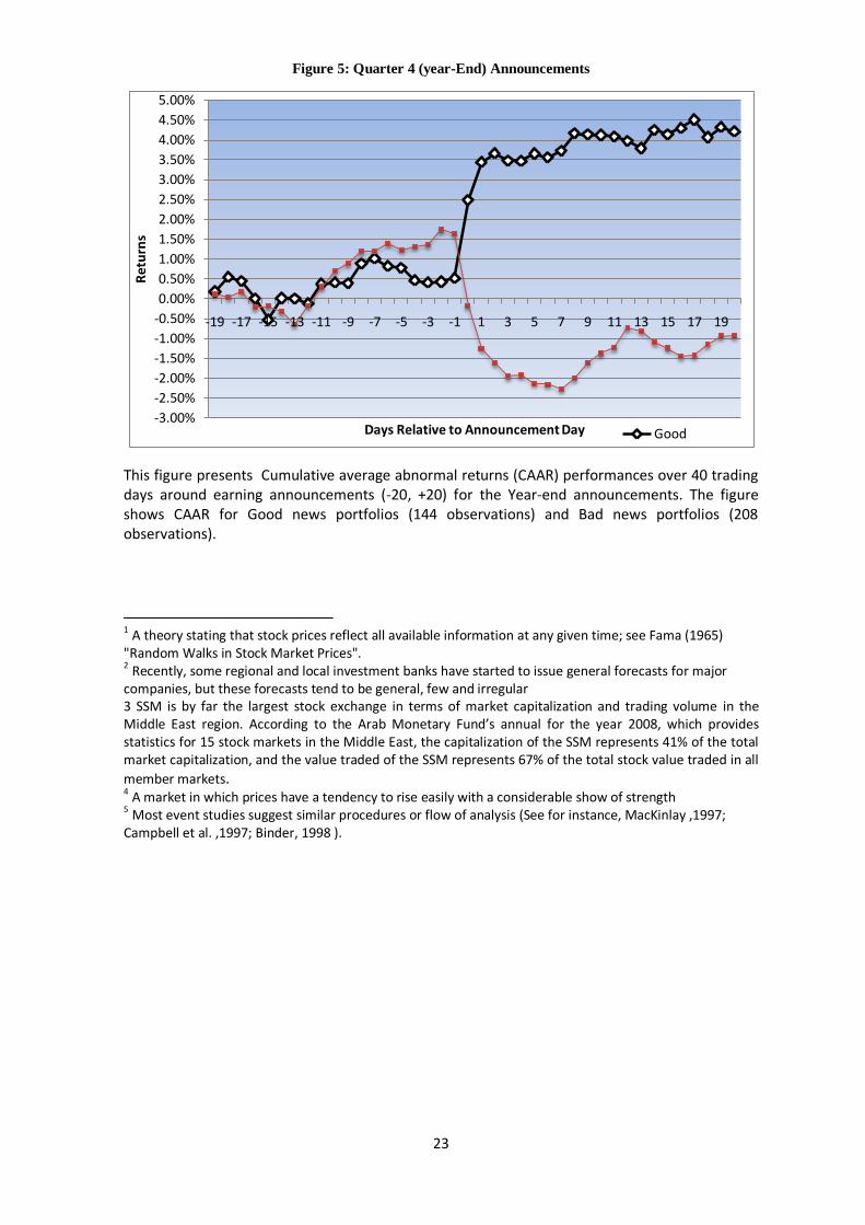
This figure presents Cumulative average abnormal returns (CAAR) performances over 40 trading days around earning announcements (-20, +20) for the Year-end announcements. The figure shows CAAR for Good news portfolios (144 observations) and Bad news portfolios (208 observations).

1 A theory stating that stock prices reflect all available information at any given time; see Fama (1965) "Random Walks in Stock Market Prices". 2 Recently, some regional and local investment banks have started to issue general forecasts for major

companies, but these forecasts tend to be general, few and irregular 3 SSM is by far the largest stock exchange in terms of market capitalization and trading volume in the Middle East region. According to the Arab Monetary Fund’s annual for the year 2008, which provides statistics for 15 stock markets in the Middle East, the capitalization of the SSM represents 41% of the total market capitalization, and the value traded of the SSM represents 67% of the total stock value traded in all

member markets. 4 A market in which prices have a tendency to rise easily with a considerable show of strength

5 Most event studies suggest similar procedures or flow of analysis (See for instance, MacKinlay ,1997; Campbell et al. ,1997; Binder, 1998 ).

-3.00%

-2.50%

-2.00%

-1.50%

-1.00%

-0.50%

0.00%

0.50%

1.00%

1.50%

2.00%

2.50%

3.00%

3.50%

4.00%

4.50%

5.00%

-19 -17 -15 -13 -11 -9 -7 -5 -3 -1 1 3 5 7 9 11 13 15 17 19

Re

turn

s

Days Relative to Announcement Day Good