how many people are in your future? - academicsacademics.smcvt.edu/gashline/papers/99 mcgraw-hill...

HHOOWW MMAANNYY PPEEOOPPLLEE AARREE IINN YYOOUURR FFUUTTUURREE??

ELEMENTARY MODELS OF POPULATION GROWTH

George L. Ashline, Assistant Professor of Mathematics Joanna A. Ellis-Monaghan, Instructor of Mathematics

Saint Michael’s College The Case

The year is 2022 AD. Forty million people crowd New York City. An air-locked plastic bubble preserves the small handful of sickly trees remaining. Bodies pack stairwells at night. Only the very wealthy can afford fresh vegetables, strawberry jam, or even hot running water. Teeming masses of desperate people mill around derelict cars on filthy streets, wearing surgical masks against the thick yellow smog. They fight for crumbs of government-supplied protein crackers, and bulldozers control daily food riots, scooping crying, starving people into bloody piles. Sanitation trucks soon arrive for routine collection of the dead.

Is this your future? How would you know whether or not it is? Should you believe people who say it is your future? Background The scenario above depicts the future portrayed in the 1973 dystopian science fiction classic Soylent Green [F]. But why would anyone think this is a realistic model of the future? Who would predict such population growth and on what basis? In the prologue to the 1966 book Make Room! Make Room!, which was the basis for Soylent Green, the author Harry Harrison writes that

…within fifteen years, at the present rate of growth, the United

States will be consuming over 83 per cent of the annual output of the earth’s materials. By the end of the century, should our population continue to increase at the same rate, this country will need more than 100 per cent of the planet’s resources to maintain our current living standards. This is a mathematical impossibility--aside from the fact that there will be about seven billion people on this earth at that time and--perhaps--they would like to have some of the raw materials too.

In which case, what will the world be like?

Ashline and Ellis-Monaghan 1999

Given that it is now more than fifteen years (in fact more than thirty years) since the book was published, what do you think of Harrison’s prediction? Harrison’s statement shows that he based his vision of the future on an exponential model of human population growth. Throughout history many people have, either deliberately or out of ignorance of other models, chosen to use a particular population model specifically to make a case for a particular point of view. For example, Paul Ehrlich, in The Population Bomb, uses an exponential model to predict that in 900 years world’s population will be 60,000,000,000,000,000, or 100 people per square yard of the earth’s surface, land and sea. ([E], p. 18). He then uses this dire prediction to justify such draconian measures as involuntary sterilization of the general population through contraceptives in the water supply, with the antidote “carefully rationed by the government to produce the desired population size” ([E], p. 135), although he admits such measures would be difficult to enforce.

In fact, not only are populations in many parts of the world not growing

exponentially, they aren’t even growing—they are declining. The replacement growth rate (the rate needed for an unchanging population) is about 2.2 children born to each woman. ([C], p. 288). However, in 1997, the rate in both Spain and Italy was only 1.2 children per woman. Europe as a whole is well below replacement level, with an average total fertility rate of 1.4. Even the U. S. is only at 2.0 children per woman ([PRB]). Many other countries have fertility levels below the replacement level and it is expected that this trend will also eventually manifest in many of the remaining countries. ([T], pp. 168-169). So, although exponential models can be very helpful if used appropriately, (and these models will be developed in this case study), as Cohen points out, they have repeatedly failed as good forecasters of long term population growth.

Because of its great simplicity, the exponential model is remarkably useful for very short-term predictions: the growth rate of a large population during the next one to five years usually resembles the growth rate of that population over the past one to five years. Because of its great simplicity, the exponential model is not very useful for long term predictions, beyond a decade or two. Surprisingly, in spite of the abundant data to the contrary, many people believe that the human population grows exponentially. It probably never has and probably never will. ([C], p. 84).

Why is population growth such an urgent concern? Who wants to know? And

why is it so hard to predict? Haub addresses the first two questions:

Interest in [population] projections involves much more than a simple curiosity about what may lie ahead. Having some sense of the number of people expected, their age distribution, and where they will be living provides city planners and local governments, for instance, sufficient “lead time” to prepare for coming needs in terms of schools and


traffic lights, or reservoirs and pipes to deliver water supplies. Businesses have a vital interest in the coming demand for their products and services.” ([H], p. 3).

World population projections have been a cause of considerable concern, particularly because of the population “explosion” of the post-World War II years. The probable consequences of rapidly expanding human numbers have been the subject of lively debate. Recently, that debate has been joined in controversy by the issue of population decline resulting from the very low birth rates in some countries. Books on these concerns range from Paul Ehrlich’s “The Population Bomb” to Ben Wattenberg’s “The Birth Dearth.” ([H], p. 4).

Despite the urgency of the questions, answers to human population concerns are hard to determine. Complicating the prediction process is the fact that the forecasters may themselves be biased, influencing their choice of models and their basic assumptions. As Simon notes,

…several groups have had a parochial self-interest in promoting these doom-saying ideas [of explosive population growth leading to scarce resources]. …these groups include (a) the media, for whom impending scarcities make dramatic news; (b) the scientific community, for whom fears about impending scarcities lead to support for research that ostensibly will ease such scarcities; and (c) those political groups that work toward more government intervention in the economy; supposedly worsening scarcities provide an argument in favor of such intervention.” ([S], pp. 3-4). Demographers honestly admit that they can not predict the future: “Here is one of

the best-kept secrets of demography: most professional demographers no longer believe they can predict precisely the future growth rate, size, composition and spatial distribution of populations.” ([C], pp. 109-110). Furthermore, any mathematical model hoping to predict future conditions can only assume that existing trends will continue unchanged or will change in a predictable way. This is a very tenuous assumption, especially regarding such factors as fertility and mortality rates. But decisions must be made, by the business community, by governments, by policy makers, and by individuals. These decisions depend on estimates of future conditions. If you needed to predict population trends, to allocate resources for example, how would you do it? And how would you argue for the effectiveness of your models?

In order to address these questions, it’s first necessary to know what models are

available, and why you should think that they could be applied to human population changes. During this course, you will examine models given by the exponential and logistic curves. After collecting data from laboratory cultures of various organisms, you will see that both functions are quite effective models of population growth in the


microcosm of the laboratory experiment. In fact, both can even give quite accurate predictions of future growth. Because these two curves so accurately model other organisms, it seems likely that they can offer useful information about the human condition as well. Like other more sophisticated models (such as the cohort methods not discussed here), the exponential and logistic curves have limitations as long range forecasters of human populations. However, they are both very good for short-term predictions, and they are especially good for backward analysis.

People themselves create the major difficulty in applying these models to the human condition. Unlike bacteria in a laboratory which simply reproduce until they have exhausted all available nutrients, humans have highly complex value systems which effect their reproductive trends and use of resources.

Humans seem to resolve conflicts of values by personal and social processes that are poorly understood and virtually unpredictable at present. How such conflicts are resolved can materially affect human carrying capacity, and so there is a large element of choice and uncertainty in human carrying capacity. … Not all of those choices are free choices. Natural constraints restrict the possible options…. ([C], p. 296).

Because of this,

Estimating how many people the Earth can support requires more

than demographic arithmetic. …it involves both natural constraints that humans cannot change and do not fully understand, and human choices that are yet to be made by this and by future generations. Therefore the question “how many people can the Earth support?” has no single numerical answer, now or ever. Because the Earth’s human carrying capacity is constrained by facts of nature, human choices about the Earth’s human carrying capacity are not entirely free, and many have consequences that are not entirely predictable. Because of the important roles of human choices, natural constraints and uncertainty, estimates of human carrying capacity cannot aspire to be more than conditional and probable estimates…. ([C], pp. 261-262).

In this course, aspiring only to ‘conditional and probable estimates’, you will develop the necessary mathematical tools to understand exponential and logistic curves. You will conduct laboratory experiments using various organisms, then use the models to analyze the growth of these cultures. Human population data will be collected from a variety of sources, including internet sites giving the most up-to-date information currently available. Having gained some confidence in the effectiveness of the models from your experience with laboratory-grown organisms, you can then apply them to the human populations of various countries. You’ll be able to check your short-term predictions against known results and use the new data to refine your models. Finally you will use your models to predict future populations, both for individual countries and


for the entire world population. Internet resources are available to see how your predictions compare to the most recent estimates of professional demographers. So, is Soylent Green your future? By the end of this course, you should be able to make an educated assessment as to whether or not you should be stocking up on strawberry jam and surgical masks.

Bibliography

[C] Cohen, Joel E., How Many People Can the Earth Support? 1995, W. W. Norton and Company, New York, London.

[E] Ehrlich, Paul R., The Population Bomb, 1968, Ballantine Books, New York.

[F] Fleischer, Richard, dir. Soylent Green. With Charleton Heston, Leigh Taylor-Young, Chuck Connors, Joseph Cotten, Edward G. Robinson. MGM, 1973.

[Har] Harrison, Harry, Make Room! Make Room!, 1966, Gregg Press, Boston.

[H] Haub, Carl, “Understanding Population Projections”, Population Bulletin, Vol. 42, No. 4, December 1987.

[PRB] Population Reference Bureau, 1997 World Population Data Sheet, 1997.

[S] Simon, Julian L., Population Matters, 1990, Transaction Publishers, New Brunswick.

[T] Tapinos, Georges and Piotrow, Phyllis T., Six Billion People, 1980, McGraw-Hill Book Company, New York.



Global Teacher’s Notes

Objectives and Overview of the Case Study The main objective of this case study is to give students interesting, motivating

contexts for the material in a first semester calculus course. The students become possessive of and involved in their own data—their yeast cultures, their chosen country’s census information. Concepts such as rate of growth, concavity, differential equations and area then have a physical context that personally interests the students. Students also gain greater appreciation of the technological resources available to them. A student confronted with the computational tedium of manipulating real data quickly realizes the value of a CAS or graphing calculator. Similarly, a student exploring the effects of changing birth and death rates in Nigeria is as quickly impressed with the population resources available on the World Wide Web.

This case study also demonstrates how a mathematical model can address

complex questions and yield answers simply not discernible from the raw data alone. This strongly motivates the use of modeling and the importance of mathematics in studying biological and sociological issues (and, by extension, issues in other fields). Furthermore, in proceeding from microbiology to demography, students see the use of laboratory experiments as a microcosm for larger questions, and they experience the process of questioning and validating mathematical techniques. These experiences give them a taste and a vision of how this class is likely to be useful to them in any chosen career or endeavor.

The biology experiments in this study are tailored to illustrate the growth

functions typically encountered in the calculus course. For example, in addition to the experiments using microorganisms, there are experiments using slime molds and flour beetles which demonstrate exponential growth. Also exponential and logistic growth can be empirically studied in projects using ciliated protistans and/or yeast cultures with varying nutrient levels. Finally, for the sake of comparison, sustained growth can be modeled using pond water.

After empirically analyzing biological growth, a major research project toward the end of the case study allows students to investigate how their laboratory results can be extended to the question of human population growth. This leads students to begin to grapple with the highly complex issue of human population modeling. There are also references later in this section to some resources with dramatically different population projections for students to consider at the beginning of the case study and then to discuss at the end in light of what they have learned.


The final project involves synthesizing all the important concepts students have learned throughout the course, and then applying them in the area of demography. Students choose a country or geographic region and then use a variety of library resources and electronic tools such as the internet and IntlPop (a demographic projection software package) to gather data. This information is used to develop and then refine population models for the countries. Hopefully, students will discover some of the inherent difficulties of modeling human population change as they compare their results with known census reports. But as they interpolate and extrapolate based on their data and models, they will also learn a real respect for the power of mathematical modeling, and the value of the mathematical skills they learned in calculus. When to Introduce the Case Study

Ideally, this case study would be run throughout a first semester calculus course. Some lab experiments take several weeks to develop growth patterns, and these should be started at the beginning of the course. Others take as little as a few days to complete. Meaningful discussion of the data from these labs can begin after the definition of the derivative has been developed and various properties and examples of derivatives have been considered. The study is designed to give a context for and hands-on experience with central concepts such as derivatives, exponential and logarithmic functions, properties of graphs, and integration in roughly the order that they are introduced in a standard elementary calculus course.

Necessary Concepts The following concepts are necessary to this case study. Students must either be familiar with them before beginning it, or they should be learning them concurrently with it.

1. Dependent vs. independent variables; 2. Functions and their basic properties, examples of functions; 3. Graphs of functions and interpretations of such graphs; 4. Asymptotes of graphs (horizontal asymptotes needed for logistic growth

models); 5. Slopes of graphs, increasing vs. decreasing functions; 6. Shapes of graphs, concave up (increasing at an increasing rate or decreasing at

a decreasing rate) vs. concave down (increasing at a decreasing rate or decreasing at an increasing rate), inflection points of graphs;

7. Limits and their basic properties and examples; 8. Rates of change, average vs. instantaneous velocities; 9. Slopes of secant lines and tangent lines; 10. The derivative of a function, examples and properties;


11. Inverse functions, exponential and logarithmic functions; 12. Derivatives of exponential and logarithmic functions; 13. Integration of exponential and logarithmic functions.

Use of Technology As previously mentioned, several of the major components of this case study offer opportunities to integrate technology. The level of integration will depend upon the resources available to the teacher, but a certain level of technology is necessary for the success of the case study. Ideally, the in-class demonstrations in this study should be replicated in the classroom using whatever technology (CAS or graphing calculator) is available. However, if necessary, they can also simply be reproduced on an overhead and discussed in class. In particular, students must have access to a graphing calculator or CAS which assist in the calculation and interpretation of various parts of the case study. Additionally, as they investigate their final research topics concerning human population projections, internet access will be very useful.

Sample Population Internet Sites

Note: Addresses of internet sites change frequently, as do the sites themselves. If any of the following sites become invalid, many similar sites will still be available and can be found using a web browser.

http://www.census.gov/ Home page of the US Census Bureau Provided by the U.S. Census Bureau, this site offers a rich collection of social, demographic, and economic information. For example, one can search for population information indexed by word, place, or a clickable map. Using the place search and the “U.S. Gazetteer”, one can obtain 1990 census data for various towns, cities, and counties throughout the United States.

http://geosim.cs.vt.edu/ Home page of Project GeoSim at Virginia Tech Project GeoSim is a research project of the Departments of Geography and Computer Science at Virginia Tech. Many educational modules for introductory geography courses have been created through this project. Two such modules include HumPop and IntlPop. HumPop is a multimedia tutorial program introducing and illustrating population concepts and issues, while IntlPop is a useful population simulation program for the various countries and regions around the world.


http://www.nidi.nl/links/nidi6000.html Home page of NiDi Maintained by the Netherlands Interdisciplinary Demographic Institute, this site offers a comprehensive overview of demographic resources on the internet. It contains over 370 external links to various useful sites on software and demographic models, demographic research institutes and organizations, etc.

http://www.popnet.org/ Home page of Popnet Created by the Population Reference Bureau, Popnet offers links to many sites containing global population information. For example, it contains links to organizational sources in many countries throughout the world, offers various demographic statistics, and includes a “demographic news update”. It also contains a clickable world map through which the user can obtain a directory of websites that provide region specific information. http://www.prb.org/ Home page of the Population Reference Bureau (PRB) The Population Reference Bureau is a nonprofit, nonadvocacy organization which is “dedicated to providing timely, objective information on U.S. and international population trends”. The PRB has been providing information about demographic trends shaping the world since 1929. http://www.iisd.ca/linkages/ Home page of Linkages Provided by the International Institute for Sustainable Development (IISD), which publishes the Earth Negotiations Bulletin, Linkages is “designed to be an electronic clearing-house for information on past and upcoming international meetings related to environment and development”. For example, it contains a link (http://www.iisd.ca/linkages/cairo.html) to the home page of the 1994 Cairo International Conference on Population and Development.

http://popindex.princeton.edu/ Home page of the Population Index Created by the Office of Population Research at Princeton University, the Population Index presents an “annotated bibliography of recently published books, journal articles, working papers, and other materials on population topics”. It contains an on-line database (for 1986-1997) which can be searched by author, geographical region, subject matter, and year of publication. http://coombs.anu.edu.au/ResFacilities/DemographyPage.html

Home page of Demography and Population Studies at ANU Provided by the Coombs Computing Unit in the Research Schools of Social Sciences & Pacific and Asian Studies at the Australian National University, this site contains 155 links to demographic information centers and facilities world-wide. These include links to various demography and population studies WWW servers, databases of interest to demographers, and demography and population studies gopher servers. Many excellent sites can be found using this Home page.


gopher://SJUVM.STJOHNS.EDU:70/11/discipln/business/census Census & demographic data

Maintained by St. John’s University, this gopher site offers 1990 demographic data for every state in the United States. Census information for each state includes total population and population breakdowns according to sex, age, and race. Data is also given for the various types of households found in each state.

Supplementary Resources

Alonso, William and Starr, Paul (editors), The Politics of Numbers, The Russell Sage Foundation, New York, 1987.

Ehrlich, Paul R., The Population Bomb, 1968, Ballantine Books, New York. Fleischer, Richard, dir. Soylent Green. With Charleton Heston, Leigh Taylor-

Young, Chuck Connors, Joseph Cotten, Edward G. Robinson. MGM, 1973. (available on videocassette)

Glase, Jon C. and Zimmerman, Melvin, “Population Ecology: Experiments with

Protistans”, Experiments to Teach Ecology, pp. 37-69, Ecological Society of America, Tempe, AZ, 1993.

May, Robert M. (editor), Theoretical Ecology Principles and Applications, W.B.

Saunders Company, Philadelphia, 1976. Seeley, Harry W. and VanDemark, Paul J., Microbes in Action, pp. 82-83, W.H.

Freeman & Company, San Francisco, 1981. Shryock, Henry S., Siegel, Jacob S., and Associates, The Methods and Materials

of Demography (Volume 2), U.S. Bureau of the Census, Washington D.C., 1973.

Simon, Julian L., Population Matters, 1990, Transaction Publishers, New

Brunswick. Fleischer, Richard, dir. Soylent Green. With Charleton Heston, Leigh Taylor-

Young, Chuck Connors, Joseph Cotten, Edward G. Robinson. MGM, 1973.



Preliminaries

Teacher’s Notes At the outset of this case study, the following activities begin. • Distribution of scenes from the science fiction movie Soylent Green to begin

discussion of motivating sociological and political issues surrounding population changes.

• Assignment of background reading, perhaps containing dramatically different

population projections, to illustrate some of the difficulties in forming accurate demographic predictions (see The Politics of Numbers, by Alonso and Starr, for example).

• Set up of the experiments to be used in the case study. Some of the biology

experiments can take up to several weeks to run. It is important to set them up at the beginning so that students can collect data for their final projects throughout the course. Information for setting up and running the experiments follows. There is also a student handout for recording data.

• Introduction to the technology that will be used within the case study. In order to do

the exercises associated with this study, students need to be able to use the available technology (CAS, graphing calculators, etc.) to perform basic equation and function manipulations. In particular, they must be able to use the technology to solve equations and systems of equations, and to find the roots of functions. They must be able to differentiate and to verify solutions of differential equations. They must also be able to plot points and graph functions. The student worksheet at the end of this section will verify that they have the necessary skills to continue.

• Discussion of some of the necessary mathematical concepts, including asymptotes,

increasing vs. decreasing functions, extrema, concavity, inflection points.


Laboratory Notes

In this case study, various types of population growth will be simulated and examined under controlled conditions and environments. Below is the basic information for each lab which can be included in this study. For each experiment, the equipment needed is listed and the procedure is specified. If there isn’t time or facilities to do all of the experiments, it suffices to choose one example of exponential growth and one of logistic growth. If absolutely necessary, student participation in the experiments can be omitted. In this case, the teacher must simply provide the students with appropriate raw data.

The populations studied include slime molds (to qualitatively model exponential growth), flour beetles (to model exponential growth), yeast cultures (to model both exponential and logistic growth), ciliated protistans (to model exponential and logistic growth), and pond water organisms (to model sustained growth as a supplementary experiment).

Some of the materials needed can be obtained at a grocery store. Other items can

be ordered from biological supply companies, such as the following:

Carolina Biological Supply Company 2700 York Road Burlington, NC 27215 1 (800) 334-5551 Connecticut Valley Biological 82 Valley Road, P.O. Box 326 Southampton, MA 01073 1 (413) 527-4030

I. Modeling exponential growth with slime molds and flour beetles Equipment needed

• Slime molds • Non-nutrient agar (2% agar) • Oatmeal • Petri dishes Slime Mold Procedure:

The slime molds are grown in a petri dish on sterile agar with oatmeal sprinkled on top. When the slime molds run out of oatmeal, they will move out in search of food. The actual timing of this “migration” will depend on how much food is initially given to them (this could even become the basis of an experiment,


if so desired). It will most likely take at least 2 weeks for the slime molds to begin migrating. The experiment with flour beetles is outlined in Part B of Glase and Zimmerman’s “Population Ecology: Experiments with Protistans”. (See Supplementary Resources at the end of the Global Teacher’s Notes). The beetles provide a good example of exponential growth, but a difficulty with this experiment is that it takes upwards of 7 weeks to get a good illustration of this growth.

II. Modeling exponential/logistic growth with a yeast culture A yeast culture will exhibit exponential growth during the first 10 to 36 hours of the experiment and logistic growth if the experiment continues for 48 hours.

Equipment needed

• culture tubes containing 15 ml of YPD broth (consisting of 1% yeast extract, 2% peptone, and 2% dextrose)

• Counting chamber (A spectrophotometer can also be used.) • Microscope (400X) • Yeast culture (Dry yeast available in grocery stores can be used.) • Orbital shaker

Yeast Procedure: Add one grain of dried yeast to 15 ml of sterile YPD in a culture tube. Gently dissolve the yeast grain. Incubate the tube at room temperature, or for faster growth at 30o C. Periodically (and at least at the beginning of the experiment), remove 10 ul of broth and place on the counting chamber. At room temperature, observations should be made every 4 hours or so. Count the number of cells to determine the concentration of yeast cells. The small squares of the counting chamber have an area of 1/400 mm2. The depth of the liquid is 1/50 mm. Cell concentration is reported as cells/ml. If a spectrophotometer is used, then the absorbance of the culture can be measured at 600 nm.

III. Modeling logistic growth with a bacterial culture This is perhaps the least complicated of all the experiments. In this experiment bacterial cultures get restricted nutrients and exhibit logistic growth. The amount of time needed to see the logistic growth will depend upon the incubation temperature of the agar plates. At 35°C, it could take 24 to 36 hours, whereas at room temperature it may require days.


Equipment needed • Bacterial culture (Bacillus subtilis) • Tryptic soy agar plate (DIFCO) • Ruler

Bacterial Procedure: Streak out Bacillus subtilis on a tryptic soy agar plate (DIFCO) such that you will obtain well-separated colonies. To accurately measure colony growth, it may be most effective to grow a single culture on a single plate. The plates can be incubated at either room temperature or 35°C, depending upon how quickly you want growth. At room temperature, observations should be made about once a day. The diameters of the resulting bacterial colonies can be measured with a ruler.

IV. Population crash with ciliated protistans

This experiment allows students to observe exponential and logistic growth followed by a precipitous decline or “crash” in population using a few different species of ciliated protistans.

Equipment needed • Handout entitled “Population Ecology: Experiments with Protistans” • Protistan cultures • Stereoscopic binocular microscope • Pasteur pipettes and bulbs • Volumetric pipettes and dispensers • Depression slides and counting plates • Sterile spring water • Culture vials and plugs • Concentrated liquid food

Protistan Procedure:

The experimental procedure is outlined in detail in Part A of “Population Ecology” (see Supplementary Resources at the end of the Global Teacher’s Notes). Four to five different protistan species are available for selection. One type containing photosynthetic green algae(Paramecium bursarie) is useful in experiments of light vs. dark growth. For the purposes of this case study, it may be most worthwhile to simplify the parameters of the experiment as much as possible and to set up only single species cultures. In such cultures, the predator species Didinium would not be a feasible selection (since it is used primarily in predator/prey experiments). The “Population Ecology” handout discusses more complicated variations of a single species study, such as predator/prey and


competition experiments, which may be worthwhile if time permits. Protistan cultures are grown in culture vials and pp. 42-43 of “Population Ecology” give precise and detailed techniques for counting individual organisms. For example, after thoroughly mixing the vials, Pasteur pipettes are used to place a sample of the cultures onto counting plates for microscopic inspection. Using these methods, protistan growth can be closely monitored and then modeled.

V. Modeling sustained growth with pond water (supplementary)

Equipment needed

• Screwcap test tube • Water and mud (stones removed) from lake or pond • Shredded paper/powdered cellulose • Salts of sulfate, carbonate, and phosphate • Pasteur pipette • Microscope

Pond Water Procedure:

The experimental procedure is given in the “Microbes in Action” (see Supplementary Resources at the end of the Global Teacher’s Notes). It outlines the construction of a small ecological system known as a Winogradsky column which simulates microbial processes (such as those occurring in the water/mud of a lake/pond/river). The column is a clear container (like a test tube) which is packed with shredded paper (for energy and carbohydrate); lake mud mixed with salts of sulfate, carbonate, and phosphate; and water. One of the difficulties with this experiment is that it takes quite a bit of time to complete. An incubation period of 2-3 weeks (with the column covered) is needed to eliminate any presence of algae. Another several weeks of incubation with the column uncovered near a light source is needed for microorganisms to grow. During this period, a Pasteur pipette can be used to sample the column and examine the growth microscopically. Also, macroscopic examinations can be made throughout the experiment to detect changes in the column.


Student Handout – Data Recording During the course of this class you will collect data from several laboratory experiments. For each experiment, record your data in a table like the one below. Name: Course/Section: Experiment: Organism observed: Measurement method: Observation # Date and Time # of Hours (in

decimals) Observation

Comments:


Student Handout – Exercises

The following exercises are for you to practice using either a CAS or graphing calculator to do the types of computations which are likely to arise as you work on this case study. 1. Solving equations, finding roots of functions, and solving systems of

equations.

a) Solve for x: . 0642 =−− xxb) Solve for x: . 02 =++ cbxax

c) Find the roots of the following function by setting the function equal to zero and

then solving: ( ) x. xxh 33 −=

d) Roots of functions can determine the time when something happened. For example, if ( ) ( ) e . tf t.- 20302= is the concentration of a drug in the blood at time t, then you can find the time at which the concentration was 2.9 milligrams by finding the roots of . ( ) 92.tf −

Determine at what time the concentration of the drug is 1.3 milligrams, and interpret your solution.

e) Solve the system of equations: 122353 =−−= xy, x y .

f) You should be able to solve systems of equations involving exponential

expressions, finding the initial value and the growth constant. For example, suppose that a bacterial culture is growing exponentially. Also, assume that 1 hour after the experiment begins, there are 200 thousand bacteria present and that 2.5 hours after, there are 265 thousand. Then, you should be able to find the constants in by solving ( ) ktCetp = ( ) 2001 =p and ( ) 2655.2 =p for C and k.

Find the constants C and k discussed above.

g) Unfortunately, when very large or small numbers are involved your graphing calculator or CAS may give you an error message. For example, try solving

and for C and k, where ( ) 2001 =p ( ) 95026 =p ( ) ktCetp = . If you get an error message using the technique above, you can still solve for k by using the fact that

for exponential functions the growth constant is equal to 21

21 )ln()ln(tt

AA−− , where

A1 is the amount at time t1 and A2 is the amount at time t2. Thus, you can first

find 261

)950ln()200ln(−−

=k , and then solve for C.

Find the constants C and k discussed above.


2. Differentiation.

a) Differentiate . ( ) 23 xxxf −= b) Differentiate with respect to t. ( ) ktCetg =

c) Show that ( ) ( )kteMtv −−= 1 is a solution to the differential equation

)( vMkdtdv

−= .

3. Graphing.

a) Graph xexf =)( .b) Graph , where kxCexg =)( 18.2 and ,0386.0 == kC .

c) Graph MktBeMth −+

=1

)( , where 18.0 and ,5.21 ,32 === kBM .


Student Handout – Solutions

1. Solving equations, finding roots of functions, and solving systems of equations.

a) 102,102 −+ .

b) aac

24bb 2−+−

, aac

24bb 2−+

.

c) 3,3 ,0 − .

d) t = 2.852724293. The solution indicates that about 2 hours and 54 minutes later the concentration of the drug will be 1.3 milligrams.

e) 746 ,

727

== yx , or in decimal form: y = 6.571428571, x = 3.857142857.

f) C = 165.7878668, k = 0.1876083063.

g) C = 187.9153474, k = 0.0623257847 .

2. Differentiation.

a) 3x2 – 2x.

b) )()( ktCketgdtd

=.

c) To verify that )( vMkdtdv

−= , we calculate the derivative of ( ) ( )kteMtv −−= 1 .

We find that )()( vMkMkedtdv kt −== − , as required.


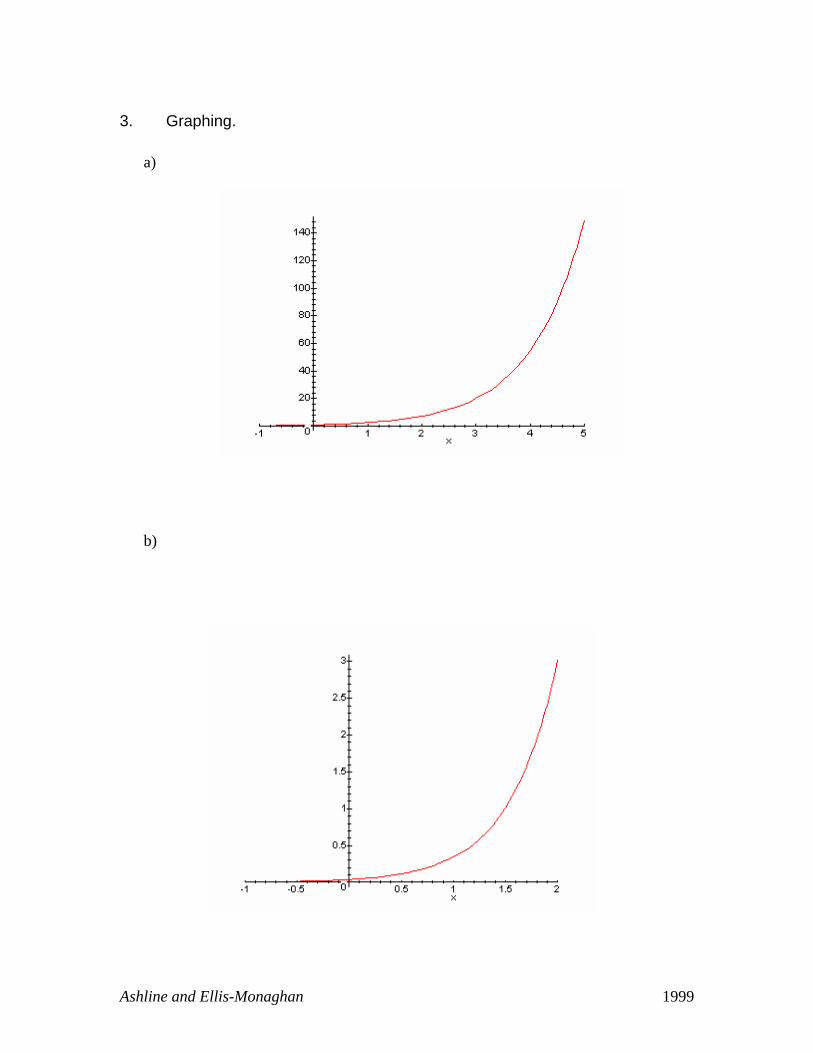
3. Graphing.

a)

b)


c)



Exponential Growth

Teacher’s Notes Introduce the exponential growth model at this point in the case study. This model describes the population growth observed in several of the ongoing experiments, particularly the slime molds, flour beetles, and yeast cultures. This section involves the following activities:

• Motivation of the exponential function as a basic tool for modeling population growth.

• Introduction of the exponential function , its basic properties, and its derivative being itself (which can be verified empirically by plotting the slopes of the tangent lines at any domain value and noticing that the resulting function is the same as the original function).

e x

• Discussion of inverse functions and their basic properties. • Consideration of the natural logarithm function ln( x ) as the inverse to

(logarithms are especially important if ecological experiment with protistans is to be used in this case study). e x

• Introduction to differential equations and, in particular, the differential equation to which ′ =y y

yy e x= is a solution.

• Description of exponential growth via the differential equation with initial condition

′ =y ky C( )0 = , which has a solution . y Cekx=

• Realization that real world phenomena are modeled by the exponential function (examples include a bacterial culture which grows at a rate proportional to its size).



1. a) Show that satisfies the differential equation ktCey = kyy =′ .

b) Show that MktBeMty −+

=1

)( satisfies the differential equation = ky(M – y). ′y

2. Suppose a yeast culture has 1.2 thousand organisms present at 10:00 a.m. on Tuesday, and 3.6 thousand at 1:45 p.m. on Friday, and assume the culture is growing exponentially.

a) Find a function P(t) for the number of yeast organisms present t hours after noon on Monday (remember to convert hours into decimals).

b) How many organisms were present initially (i.e. at noon on Monday)?

c) What is the growth constant?

d) How many organisms were there at noon on Wednesday?

e) When will there be 5 thousand organisms present?

f) How fast will the population be growing at that time?

g) How long does it take for the population to double in size?

3. Graph P(t) and use it to check your answers in Exercise 2.



1. a) To verify that )(tkydtdy

= , we calculate the derivative of ( ) ktCety = . We find that

)(tkykCedtdy kt == , as required.

b) To verify that )( yMkydtdy

−= , we calculate the derivative of MktBeMty −+

=1

)( .

We find that ))()(( tyMtkydtdy

−= , as required.

2. a) tetp 014503125.08721905501.)( =

b) C = .8721905501

c) k = .01450313251

d) p(48) = 1.749627665

e) t = 120.4005597, or Saturday at 12:24 p.m.

f) ′P (120.4) = .07251507396

g) t = 47.79292888, or about 47 hours and 48 minutes 3.



Logistic Growth

Teacher’s Notes

The logistic curve models the restricted population growth observed in several of the ongoing experiments, including those involving yeast cultures (with restricted nutrient levels) and ciliated protistans. The following activities accompany this part of the case study.

• Review of concavity and inflection points of curves as well as horizontal asymptotes of graphs.

• Introduction of the logistic curve and its mathematical properties, including the significance of its concavity changes and horizontal asymptote (called the carrying capacity of the environment).

• Illustration of the characteristics of logistic growth with some real world examples (such as disease epidemics).

• Comparison of exponential growth (growth rate proportional to the population size), limited growth (growth rate proportional to distance between the size of the population and the carrying capacity), and logistic growth which is a combination of exponential and limited growth (growth rate proportional to the size of the population and the distance between the size of the population and the carrying capacity).

• Construction of a logistic curve model by using some data points to compute curve parameters and checking the accuracy of the resulting model with other data points.

• Introduction of the notions of an integral and the average value of a function (to measure average population growth).


In-class demonstration – Growth Curves Exponential growth: This models unrestricted growth, where the rate of growth is proportional to the amount present. The function y = Cekt, where C is the initial amount and k is the growth constant, satisfies the differential equation ′y = ky. For example, here is a plot of y(t)=Cekt where C = 5.05, and k = .023.

Limited growth: The limited growth curve models limited growth, where the rate of growth is proportional to how close the amount is to the carrying capacity of the system. Such a curve looks like y(t) = M(1 – e-kt), where M is the carrying capacity and k is the growth constant. It satisfies the differential equation ′y = k(M – y). Here is a graph of y(t) = M(1 – e-kt) where M = 15 and, k = 1.23.


Logistic growth: The logistic growth curve models logistic growth, where the rate of growth is proportional to both the amount present and how close the amount is to the

carrying capacity of the system. A logistic model looks like MktBeMty −+

=1

)( , where M

is the carrying capacity, B is a number that depends on the carrying capacity and the initial amount, and k is the growth constant. It satisfies the differential equation ′y =

ky(M – y). Here is a graph of MktBeMty −+

=1

)( , where M = 25, B = 22 and k = 0.23.


In-class Demonstration – A Logistic Model

In the example below, a logistic curve is used to model the growth of a bacterial culture. The bacteria were grown in a petri dish, and every few days the diameter of the bacteria culture was measured.

Below is data collected from a bacteria culture in the spring of 1995. Here are the recorded data points: ti gives the time and di the diameter (in millimeters). The times are the number of hours (converted to decimals) after 12:45 p.m. on 4/11/95. The areas are

given by ai and computed by 4

2i

id

aπ

= .

ti di ai

t0 = 0 d0 = 2.5 a0 = 1.5625π =4.908738522 t1 = 23.16666667 d1 = 5 a1 = 6.25 π =19.63495409 t2 = 49.9167 d2 = 5 a2 = 6.25 π =19.63495409 t3 = 98.5 d3 = 6 a3 = 9.00 π =28.27433389 t4 = 148.85 d4 = 6.6 a4 = 10.8900 π =34.21194400 t5 = 167.5 d5 = 6.75 a5 = 11.390625 π =35.78470382 t6 = 192.1667 d6 = 6.52 a6 = 10.627600 π =33.38759009

Below, pairs of data points, together with an estimate for the carrying capacity M,

are used to determine a logistic function L(t) which models the growth of the bacteria. In general, a logistic curve has the following form, for some constants M, B, and

k:

)(1)( MktBe

MtL −+= .

The constant M is the carrying capacity, or limit of what the system can support.

The best way to get a preliminary estimate for M is to plot the data points and do a freehand sketch through them to estimate M. Here is a plot of the points:


That second data point looks a little too big, and the last one a little too small. This is probably because of inaccuracy in measurement. This does happen unfortunately, but we should still be able to get a good model. A good guess for the carrying capacity, M, seems to be 34.5, so

)5.34(115.34)( ktBe

tL −+= .

Now, use t0 and a0 to solve for B, getting that B = 6.028282287. Thus, L(t) looks like

)5.34(76.02828228115.34)( kte

tL −+= .

Next, use t2 and a2 to find k. Normally, we’d use t1 and a1 here, but as we noted

above, that data point looked wrong, so we went to the next one that looked good. We find that

k = 0.001204767896.

With this, L(t) looks like

)0415649241.0(76.02828228115.34)( te

tL −+= .

Now, check how well this function models the four data points. Here is what the

function L(t) gives at the times t0, t1, etc.:

ti L(ti) ai

t0 4.908738522 4.908738522 t1 10.44986633 19.63495409 t2 19.63495409 19.63495409 t3 31.34950928 28.27433389 t4 34.07758738 34.21194400 t5 34.30413399 35.78470382 t6 34.42948532 33.38759009

All but the second look pretty good. Here is the graph of L(t):


Next, here is how the actual data points fit on this curve:


With this mathematical model, we can answer some questions we couldn’t have answered just using the observed data.

I. What was the area covered by the colony at 10:00 a.m. on 4/16? First, you have to determine what t is at that time by counting 5 days less 2 ¾ hours from the start of the experiment at 12:45 on 4/11. This gives

ts = 5(24) – 2.75, or ts = 117.25. Now, evaluate L(t) at that time to find the area covered:

L(ts) = 32.97968560.

II. At what rate is the area increasing at that time? We need the derivative of L(t) to answer this. Fortunately, L(t) satisfies the differential equation y′ = ky(M – y), so we have the following formula for L′(t):

L′(t) = kL(t) (M – L(t)). Evaluate that at t to get the rate:

L′(ts) = .06040644899. III. What is the carrying capacity of the system? The carrying capacity is just M = 34.5.

IV. When does the rate slow down? In other words, when does the population stop growing at an increasing rate and start growing at a decreasing rate? (This is just asking where the inflection point is).

You can get a good estimate for this just by looking at the graph. It looks like about 43 hours after the start of the experiment.

Alternatively, you can find the second derivative of L(t), set it equal to zero and solve for t, getting that the t-coordinate of the inflection point is 43.22107658.

V. What is the average area covered by the colony during the course of the experiment?


First, we need to find the total area by integrating L(t) from t0 to t6, which gives 5012.92708. Dividing this by t6 – t0 = t6 gives that the average area covered by the colony during the course of the observed experiment is 26.08635080 mm2.


Some yeast was grown in a petri dish, and the diameter of one colony was measured, giving the following data:

date time diameter 9/3 10:00 a.m. 0.75 mm 9/4 9:10 a.m. 1.5 mm 9/5 11:55 a.m. 3 mm 9/7 12:30 p.m. 4 mm 9/9 2:51 p.m. 5.1 mm 9/10 9:30 a.m. 5.25 mm 9/11 10:10 a.m. 5.33 mm 9/12 6:15 a.m. 5.39 mm

As in the in-class demonstration, find a logistic curve to model this data, and then answer the following questions:

I. What was the area covered by the colony at 10:25 a.m. on 9/6? II. At what rate is the area increasing at that time? III. What is the carrying capacity of the system? IV. When does the rate of growth slow down? In other words, when does the

population stop growing at an increasing rate and start growing at a decreasing rate?

V. What is the average area covered by the colony during the course of the

experiment?

VI. Include a graph of the data points, a graph of your logistic curve, and a graph of the logistic curve with the data points superimposed on it.



Note: Your answers may be slightly different from these, depending on your estimate for M and which data points you used to solve for k. Here, M = 23, and t4 and a4 were used to solve for k.

I. 6.134311355 mm2.

II. 0.1814808817 mm2/hr.

III. M = 23.

IV. t = 97.48, or about 11:30 a.m. on 9/7.

V. 12.41022016 mm2.

VI. Graphs:



Biological Modeling

Teacher’s Notes

Having studied the important characteristics of the exponential and logistic models of growth, students can now apply these concepts to their own experiments. This involves the following activities.

• Completion of ongoing experiments (involving growth of yeast, slime molds, protistans, and/or pond water) and collection of last set of empirical data.

• Construction of experimental population models based on gathered results.

The handout below offers a guide for students to efficiently summarize and analyze their data. For their analysis they will fit their data using the exponential and logistic models of growth learned in this case study.


Student Handout – Lab Analysis During the course of this class you collected data from several laboratory experiments. Now, using the techniques you have learned, it is time to develop mathematical models for your experiments and use them to answer some questions which could not be answered from just the raw data. 1. For each experiment, record your data in the format given in the Student Handout –

Data Recording in the Preliminaries section. 2. Decide what kind of curve (e.g. exponential or logistic) seems to fit your data.

Explain why you chose the model you did. 3. Use the available technology (graphing calculator, CAS etc.) to get a specific

function that models your data. Your work must include the following:

a. a graph of your data points. b. work showing how you got your growth and other constants. c. a comparison between the actual data and the values predicted by your

modeling function. d. a plot of your function. e. a plot of your function with the actual data points plotted on the same graph.

NOTE: You may need to try several different values for your constants (e.g. try different data points to solve for your growth constants—even take advantage of the growth constants you get from different pairs of data points; adjust your guess for M, the carrying capacity; etc.) until you get a curve that models your data well. 4. Answer the following questions: These are questions which you could not have answered just from the experimental data, but which you can answer now that you have a mathematical model for the experiment, and the tools of calculus. Use the modeling function that you found to answer these questions. Be sure to include units and comments when appropriate in your answers. Turn in the calculations you used to find the answers to these questions. I. What are the constants you used? II. What was the area covered by the colony at 10:00 a.m. on the 5th day of the experiment? III. At what rate was the area increasing at that time?


IV. Was the rate at 10:00 a.m. on the 5th day greater or less than the rate at 10:00 a.m. on the 8th day?

V. At what time did the growth rate start slowing down? In other words, when did

the area stop growing at an increasing rate and start growing at a decreasing rate?

VI. What was the average area covered by your colony between the first measurement and the last?

VII. What do you think the population would be 24 hours after your last observation? How about 48 hours later?

VIII. Comment on your results. How well do they seem to reflect or predict reality?



Human Populations

Teacher’s Notes

After modeling the growth observed in their biological experiments, students will use similar modeling techniques to predict human population levels based on current demographic data. Students will undertake the following activities.

• Creation of human population models for various countries based on recent population levels (to test model accuracy, earlier population data can be used to project figures for years in which census data is available).

• Use of library and internet resources to gather demographic information (see the end of the Global Teacher’s Notes for addresses of some useful internet sites).

• Application of the internet program “Intlpop” (an abbreviation of “International Population”) which, for various countries/regions in the world, provides such data as recent population levels, life expectancies, fertility rates, infant mortality rates, and net migration data (other sites provide similar population data for various regions in the world and in the United States).

• Discussion of the politics of census figures and population projections leading to the realization that different sources often provide very different projections (Carl Haub’s “Understanding Population Projections” in the Population Bulletin is helpful).


Student Handout – Demographic Projections This is the final project for this case study, where you will take all the concepts learned and apply them to study the original question of human population change. 1. Choose a country that interests you, and using library or internet resources, collect as

much population data as you can prior to 1950. 2. Use this data to develop a model for the population of that country. Explain your

choice of modeling function. 3. Using your modeling function, predict the population of that country in 1960, 1970

and 1980. 4. Collect data on the actual population of your country in 1960, 1970 and 1980. What

do you think accounts for any discrepancies? 5. Use the data from the ‘80s and ‘90s to refine your modeling function. If you change

your modeling function, explain your decision. 6. Compare the actual data with the populations given by your modeling function and

see if you can find reasons for any discrepancies. How well do you think your model estimates the actual populations in 1965 and 1975? Compare your results to actual data if it is available.

7. Use your new modeling function to predict the population of your country for the

years 2000, 2010, and 2020. 8. Research population literature (including “Intlpop”) to get predictions for the future

population of your country. How do your predictions compare with those in the literature? What might account for any discrepancies (“they have a better model” is not an adequate answer—you need to discuss what factors their model considers that yours does not and to consider differences in the assumptions made).

9. How are human populations different from organisms grown in the lab? How might

the modeling functions be modified to give better predictions? BONUS: Find the population of New York City in 1973 when the movie Soylent Green was made. Develop a population model supporting the movie’s premise that the population of NYC in 2022 will be 40 million. What does your model predict that the population of NYC would have to be today? Find the most recent census data available for the actual population of NYC today and compare it to the value predicted by your model. Comment on your results.


how many people are in your future? - academicsacademics.smcvt.edu/gashline/papers/99 mcgraw-hill...

Documents