How Is Power Shared In Africa?

Patrick Francois, Ilia Rainer, and Francesco Trebbi∗

November 2012

Abstract

This paper presents new evidence on the power sharing layout of national politicalelites in a panel of African countries, most of them autocracies. We present a model ofcoalition formation across ethnic groups and structurally estimate it employing data onthe ethnicity of cabinet ministers since independence. As opposed to the view of a singleethnic elite monolithically controlling power, we show that African ruling coalitions arelarge and that political power is allocated proportionally to population shares acrossethnic groups. This holds true even restricting the analysis to the subsample of the mostpowerful ministerial posts. We argue that the likelihood of revolutions from outsidersand the threat of coups from insiders are major forces explaining such allocations.

∗University of British Columbia, Department of Economics and CIFAR, patrick.francois@ubc.ca; GeorgeMason University, Department of Economics, irainer@gmu.edu; and University of British Columbia, De-partment of Economics, CIFAR and NBER, francesco.trebbi@ubc.ca, respectively. The authors would liketo thank Daron Acemoglu, Matilde Bombardini, Ernesto Dal Bo, Raphael Frank, David Green, ThomasLemieux, Vadim Marmer, Paul Schrimpf, Eric Weese, and seminar participants at CIFAR, SITE 2012, UBCand Yale for useful comments and discussion. Chad Kendall provided exceptional research assistance. Weare grateful to the National Bureau of Economic Research Africa Success Project and to the Initiative onGlobal Markets at Chicago Booth for financial support.

1 Introduction

This paper investigates the process by which political power is shared across ethnic

groups in African autocracies. Analyzing how ruling elites evolve, organize, and respond

to particular shocks is central to understanding the patterns of political, economic, and

social development of both established and establishing democracies. For autocratic or

institutionally weak countries, many of them in Africa, it is plausible that such understanding

is even more critical (Acemoglu and Robinson (2001b, 2005), Bueno de Mesquita, Smith,

Siverson, and Morrow (2003), Wintrobe (1998), Besley and Persson (2011), Aghion, Alesina,

and Trebbi (2004)).

Scarcity and opacity of information about the inner workings of ruling autocratic elites

are pervasive. Notwithstanding the well-established theoretical importance of intra-elite

bargaining (Acemoglu and Robinson (2005), Bueno de Mesquita et al. (2003)), systematic

research beyond the occasional case study is rare.1 This is not surprising. Institutionally

weak countries usually display low (or null) democratic responsiveness and hence lack reliable

electoral or polling data.2 This makes it hard to precisely gauge the relative strength of

the various factions and political currents affiliated with different groups. Tullock’s (1987)

considerations on the paucity of data employable in the study of the inner workings of

autocracy are, in large part, still valid.

This paper presents new data on the ethnic composition of African political elites, specif-

ically focusing on the cabinet of ministers, helpful in furthering our understanding of the

dynamics of power sharing within institutionally weak political settings. Our choice of fo-

cusing on ethnic divisions and on the executive branch are both based on their relevance

within African politics and their proven importance for a vast range of socioeconomic out-

comes. First, the importance of ethnic cleavages for political and economic outcomes in

Africa cannot be overstated.3 Second, it is well understood in the African comparative poli-

1Posner (2005) offers an exception with regard to Zambian politics. Other recent studies relevant to theanalysis of the inner workings of autocracies include Geddes (2003), who investigates the role of partieswithin autocracies, and Gandhi and Przeworski (2006), who consider how a legislature can be employed asa power-sharing tool by the leader.

2Posner and Young (2007) report that in the 1960s and 1970s the 46 sub-Saharan African countriesaveraged 28 elections per decade, less than one election per country per decade, 36 in the 1980s, 65 in the1990s, and 41 elections in the 2000-05 period.

3The literature is too vast to be properly summarized here. Among the many, see Bates (1981), Berman

1

tics literature that positions of political leadership reside with the executive branch, usually

the president and cabinet.4 Legislative bodies, on the other hand, have often been relegated

to lesser roles and to rubber-stamping decisions of the executive branch5. Arriola (2009) en-

capsulates the link between ethnic divisions and cabinet composition in patrimonial states:

“All African leaders have used ministerial appointments to the cabinet as an instrument for

managing elite relations.”

We begin by developing a model of allocation of patronage sources, i.e. the cabinet

seats, across various ethnic groups by the country’s leader. We then estimate the model

structurally. Our model, differently from the large literature following the classic Baron and

Ferejohn (1989) legislative bargaining setting, revolves around nonlegislative incentives.6

This makes sense given the focus on African polities. However, similarly to Baron and

Ferejohn, we maintain a purely noncooperative approach. We assume leaders wish to avoid

revolutions7 and coups, and enjoy the benefits of power. The leader decides the size of

his ruling coalition to avoid revolutions staged by groups left outside the government and

allocates cabinet posts in order to dissuade insiders from staging a palace coup. To a first

approximation, one can think of the revolution threat as pinning down the size of the ruling

coalition (by excluding fewer groups the leader can make a revolution’s success less likely)

(1998), Bienen et al. (1995), and Easterly and Levine (1997), Posner (2004).4Africanists often offer detailed analysis of cabinet ethnic compositions in their commentaries. See

Khapoya (1980) for the Moi transition in Kenya, Osaghae (1989) for Nigeria, Posner (2005) for Zambia.Arriola (2009) considers cabinet expansion as a tool of patronage and shows cabinet expansion’s relevancefor leader’s survival in Africa. Kramon and Posner (2011) present evidence from Kenya on the large impact ofhaving a co-ethnic minister of education on educational attainment of an ethnic group. They also explicitlystate that “Scholars such as Joseph (1987), van de Walle (2007), and Arriola (2009) emphasize the extentto which presidents keep themselves in power by co-opting other powerful elites—usually elites that controlethnic or regional support bases that are distinct from the president’s—by granting them access to portionsof the state (what Joseph, following Weber, calls prebends) in exchange for their loyalty and that of theirfollowers. In practice, this is done by allocating cabinet positions, with the understanding that the holdersof those cabinet positions will use their ministries to enrich themselves and shore up their own regional orethnic support bases, and then deliver them to the president when called upon.”

5See Barkan (2009, p.2).6The literature on bargaining over resource allocation in non-legislative settings is also vast. See Ace-

moglu, Egorov, and Sonin (2008) for a model of coalition formation in autocracies that relies on self-enforcingcoalitions and the literature cited therein for additional examples. Our model shares with most of this lit-erature a non-cooperative approach, but differs in its emphasis on the role of leaders, threats faced by theruling coalition, and payoff structure for insiders and outsiders.

7Throughout the paper we use the term “revolution” to indicate any type of large-scale political violencethat pegs insiders to the national government against excluded groups. Civil wars or paramilitary infightingare typical examples.

2

and the coup threat as pinning down the shares of patronage accruing to each group (by

making an elite member indifferent between supporting the current leader and attempting

to become a leader himself). The empirical variation in size of the ruling coalition and

post allocations allows us to recover the structural parameters of the revolution and coup

technologies for each country, which in turn we employ in a set of counterfactual simulations.

Methodologically, our approach is similar to that in Diermeier, Eraslan and Merlo (2003) and

in Merlo (1997) in that we estimate a structural model of government formation. A marked

difference however arises in the theoretical approach to government formation. This reflects

the difference in the underlying forces that determine governmental stability in sub-Saharan

African regimes relative to those in parliamentary democracies that were their focus.

Contrary to a view of African ethnic divisions as generating wide disproportionality

in access to power, African autocracies function through an unexpectedly high degree of

proportionality in the assignment of power positions, even top ministerial posts, across ethnic

groups. While the leader’s ethnic group receives a substantial premium in terms of cabinet

posts relative to its size (measured as the share of the population belonging to that group),

such premia are comparable to formateur advantages in parliamentary democracies. Rarely

are large ethnic minorities left out of government in Africa, and their size does matter in

predicting the share of posts they control, even when they do not coincide with the leader’s

ethnic group.8 We show how these findings are consistent with large overhanging coup threats

and large private gains from leadership. Large ruling coalitions (often more than 80 percent

of the population are ethnically represented in the cabinet) also suggest looming threats of

revolutions for African leaders. We also show that the patterns of political inclusion follow

the precise nonlinearities predicted by our model and that the data formally reject alternative

models not relying on such mechanisms.

We do not take these findings to imply that proportionality in government reflects equality

of political benefits trickling down to common members of all ethnicities. African societies

8While these results are new, this observation has been occasionally made in the literature. Contrastingprecisely the degree of perceived ethnic favoritism for the Bemba group in Zambia and the ethnic compositionof Zambian cabinets, Posner (2005, p.127) reports “...the average proportions of cabinet ministers that areBemba by tribe are well below the percentages of Bemba tribespeople in the country as a whole, and theproportion of Bemba-speakers in the cabinet is fairly close to this group’s share in the national population.Part of the reason for this is that President Kaunda, whose cabinets comprise twelve of the seventeen in thesample, took great care to balance his cabinet appointments across ethnic groups.”

3

are hugely unequal and usually deeply fragmented. Our findings imply that a certain fraction

of each ethnic group’s upper echelon is able to systematically gain access to political power

and the benefits that follow. The level of proportionality in ethnic representation seems to

suggest that the support of critical members of a large set of ethnic groups is sought by

the leader. There is no guarantee, however, that such groups’ non-elite members receive

significant benefits stemming from this patronage, and they often do not. Padro-i-Miquel

(2007) explains theoretically how ethnic loyalties by followers may be cultivated at extremely

low cost by ethnic leaders in power. We also explore this theme theoretically in an extension

to the model developed in the Appendix to the paper.

This last point highlights an important consideration. There is overwhelming empirical

evidence in support of the view of a negative effect of ethnic divisions on economic and

political outcomes in Africa.9 The question is whether at the core of these political and

economic failures lays a conflict between ethnic groups in their quest for control, or whether

it is the result of internal struggles between elites and non-elites that arise within ethnic

enclaves. Our data show that almost all ethnic groups have access to a certain measure

of political power at the elite level. This finding argues against an overly direct view of

the relationship between ethnic fractionalization, state dysfunction and conflict, consistent

with the interpretation of Fearon and Laitin (2003). Standing ethnic divisions and cleavages

within a country are well understood by leaders, and accounted for in power allocations.

As Fearon and Laitin argue, the potential for ethnic tensions to precipitate conflict exists,

but these are best thought of as proximate determinants of actual break down. Similarly,

we demonstrate that successful leaders are able to act in ways that defuse threats to regime

coherence that would arise from underlying ethnic tensions. This finding provides indirect

evidence that frictions within ethnic groups may be playing a larger role than previously

assessed vis-a-vis frictions between groups.

Finally, by emphasizing the presence of non trivial intra-elite heterogeneity and redistri-

bution, our findings support fundamental assumptions made in the theory of the selectorate

(Bueno de Mesquita, et al. (2003)), the contestable political market hypothesis10, and in

9See Easterly and Levine (1997), Posner (2004), Michalopoulos and Papaioannou (2011).10Mulligan and Tsui, (2005) in an adaptation of the original idea in product markets by Baumol et al.

(1982).

4

theories of autocratic inefficiency (Wittman (1995)).

The rest of the paper is organized as follows. Section 2 presents our model of coalition

formation and ministerial allocations and Section 3 presents our econometric setup. Section

4 describes the data. Section 5 reports the main empirical evidence on the allocation of

cabinet posts at the group level. Section 6 presents our counterfactuals. Section 7 compares

our model to alternative modes of power sharing. Section 8 presents our conclusions.

2 Model

Consider an infinite horizon, discrete time economy, with per period discount rate δ.

There are N ethnicities in the population. Denote the set of ethnicities N = 1, ..., N.

Each ethnicity is comprised of two types of individuals: elites, denoted by e, and non-elites,

denoted by n. Ethnic group j has a corresponding elite size ej and non-elite size nj, with

ej = λnj and λ ∈ (0, 1). The population of non-elites is of size P , so that ΣNi=1ni = P .

Let N = n1,..., nN. Without loss of generality we order ethnicities from largest to smallest

e1 > e2 > ... > eN−1 > eN . Elites decide whether non-elites support a government or not.

Each elite decides support of 1/λ non-elite from its own ethnicity.

At time 0 a leader from ethnic group j ∈ N is selected with probability proportional to

group size

(1) pj (N) =exp(αej)

ΣNi=1 exp(αei)

.

Let l ∈ N indicate the ethnic identity of the selected leader and O the set of subsets of N .

The leader chooses how to allocate leadership posts (i.e., cabinet positions or ministries),

which generate patronage to post holders, across the elites of the various ethnic groups.

Let us indicate by Ωl the set of ethnic groups in the cabinet other than the leader’s group,

implying the country is ruled by an ethnic coalition(Ωl ∪ l

)∈ O. Elite members included

in the cabinet are supporters of the leader. This means that, in the event of a revolution

against the leader, the 1/λ non-elite controlled by each one of these ‘insiders’ necessarily

supports the leader against the revolutionaries11.

11In the theoretical appendix we present a derivation of the elite-nonelite bargaining problem and discussthe intra-group support decision.

5

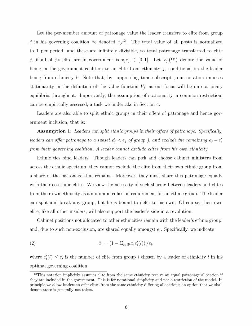
Let the per-member amount of patronage value the leader transfers to elite from group

j in his governing coalition be denoted xj12. The total value of all posts is normalized

to 1 per period, and these are infinitely divisible, so total patronage transferred to elite

j, if all of j’s elite are in government is xjej ∈ [0, 1]. Let Vj(Ωl)

denote the value of

being in the government coalition to an elite from ethnicity j, conditional on the leader

being from ethnicity l. Note that, by suppressing time subscripts, our notation imposes

stationarity in the definition of the value function Vj, as our focus will be on stationary

equilibria throughout. Importantly, the assumption of stationarity, a common restriction,

can be empirically assessed, a task we undertake in Section 4.

Leaders are also able to split ethnic groups in their offers of patronage and hence gov-

ernment inclusion, that is:

Assumption 1: Leaders can split ethnic groups in their offers of patronage. Specifically,

leaders can offer patronage to a subset e′j < ej of group j, and exclude the remaining ej − e′jfrom their governing coalition. A leader cannot exclude elites from his own ethnicity.

Ethnic ties bind leaders. Though leaders can pick and choose cabinet ministers from

across the ethnic spectrum, they cannot exclude the elite from their own ethnic group from

a share of the patronage that remains. Moreover, they must share this patronage equally

with their co-ethnic elites. We view the necessity of such sharing between leaders and elites

from their own ethnicity as a minimum cohesion requirement for an ethnic group. The leader

can split and break any group, but he is bound to defer to his own. Of course, their own

elite, like all other insiders, will also support the leader’s side in a revolution.

Cabinet positions not allocated to other ethnicities remain with the leader’s ethnic group,

and, due to such non-exclusion, are shared equally amongst el. Specifically, we indicate

(2) xl = (1− Σi∈Ωlxie′i(l)) /el,

where e′i(l) ≤ ei is the number of elite from group i chosen by a leader of ethnicity l in his

optimal governing coalition.

12This notation implicitly assumes elite from the same ethnicity receive an equal patronage allocation ifthey are included in the government. This is for notational simplicity and not a restriction of the model. Inprinciple we allow leaders to offer elites from the same ethnicity differing allocations; an option that we shalldemonstrate is generally not taken.

6

The leader also obtains a non-transferrable personal premium to holding office, denoted

by amount F . F may be interpreted as capturing the personalistic nature of autocratic

rents. Let Vj (Ω) denote the value of being in the government coalition to an elite member

from ethnicity j conditional on the leader being from ethnicity j (and the member not being

the leader himself).

Leaders lose power or are deposed for different reasons. Leaders can lose power due to

events partially outside their control (e.g. they may die or a friendly superpower may change

its regional policy). We will refer to these events as ‘exogenous’ transitions. Alternatively,

leaders can be deposed by government insiders via a coup d’etat or by outsiders via a

revolution; which are both events we consider endogenous to the model. In particular we

will search for an equilibrium in which a leader constructs a stable government by providing

patronage to elites from other ethnicities in order to head-off such endogenous challenges.

Two factors guide the allocation of patronage by the leader: 1. The leader must bring in

enough insiders to ensure his government dissuades revolution attempts by any subset of

outsiders. 2. He must allocate enough patronage to insiders to ensure they will not stage a

coup against him.

2.1 Revolutions

Revolutions are value-reducing. They lower the patronage value of the machine of gov-

ernment, but can yield material improvements to revolutionaries if they succeed in deposing

the leader. The probability of revolution success depends on the relative sizes of government

supporters versus revolutionaries fighting against them. With NI insiders supporting the

government and, for example, NO = P −NI outsiders fighting the revolution, the revolution-

aries succeed with probability NONI+NO

. This linear specification of the revolutionary contest

function does imply some loss of generality. Specifically, since only aggregates matter in the

composition of the fighting forces, the composition of ethnicities that comprise the aggre-

gates is irrelevant under this specification. We can allow for a more general contest function

where the fractionalization amongst ethnicities within the contesting forces may reduce their

effectiveness. If the insider forces include groups i ∈ NI ⊂ N and outsider forces include

i ∈ NO ⊂ N , then a more general specification of the contest function isΣi∈NOn

χi

Σi∈NOnχi +Σi∈NIn

χi,

7

which corresponds with our linear specification when χ = 1. We proceed to develop the

model with the simpler linear specification for ease of exposition, but report results for the

non-linear generalization in the Appendix.

A successful revolution deposes the current leader. A new leader is then drawn according

to the same process used at time 0, i.e. according to (1), and this leader then chooses

his optimal governing coalition. Losing a revolution leads to no change in the status of

the government. Revolutionary conflicts drive away investors, lower economic activity, and

reduce government coffers independently of their final outcome. Consequently, the total

value of all posts – normalized to 1 already – is permanently reduced to the amount r < 1

after a revolution.

Let V 0j denote the value function for an elite of ethnicity j who is excluded from the

current government’s stream of patronage rents, and V transitionj denote the net present value

of elite j in the transition state; i.e. before a new leader has been chosen according to (1).

A group of potential elite revolutionaries who are excluded from the patronage benefits of

the current government has incentive to incite the non-elite they control to revolt and cause

a revolution if this is value increasing for them. Specifically an excluded elite of ethnicity j

has incentive to instigate a revolution with NO outsiders against a government of NI insiders

if and only if: NONI+NO

rV transitionj +

(1− NO

NI+NO

)rV 0

j ≥ V 0j .

Leaders allocate patronage to insiders to buy their loyalty and hence reduce the impetus

for outsiders to foment revolution. In deciding on whether to start a revolution, elites act

non-cooperatively using Nash conjectures. That is, when an elite from an outsider group

triggers a revolution, he uses Nash conjectures to determine the number of other elites that

will join in (and hence the total revolutionary force and the probability of success) in the

ensuing civil war. Under these conjectures, once a revolution is started and all valuations

are reduced 1 − r proportionately, it follows immediately that all outsiders will also have

incentive to join the revolution. If the revolution succeeds, outsiders receive rV transitionj

which strictly exceeds rV 0j when the leader’s group wins. In short, outsiders can do no worse

than suffering exclusion from the government, their current fate, by joining a revolution once

already started.

Thus, for a revolution to not ensue, necessarily, each outsider must find it not worthwhile

8

to trigger a revolution. Since NO +NI ≡ P , it is necessary that:

(3)NO

PrV transition

j ≤(

1−(

1− NO

P

)r

)V 0j , ∀j /∈ Ωl.

It is immediate to see that this condition is easier to satisfy the greater is the size of the

ruling coalition13.

We assume that the leader suffers ψ ≤ 0 after a revolution attempt. We shall assume

throughout that ψ is large enough to always make it optimal for leaders to want to dissuade

revolutions. This assumption aims at capturing the extremely high cost of revolution for the

rulers, in a fashion similar to Acemoglu and Robinson (2001, 2005) and will make it optimal

for a leader to completely avoid revolutions.14

We also allow that insiders may start a revolution. A group of insiders from a single

ethnicity can choose to leave the cabinet and mount a revolution with their own non-elite

against the government. Again, group j ∈ Ωl decides under Nash conjectures, with the group

deviating from the ruling government unilaterally. As in all revolutions, they know that in

the revolution sub-game triggered by their deviation they will be joined by all excluded

outsiders against the leader. For a leader to ensure no such insider deviations from any of

the included ethnicities, j, yields an additional condition:

(4)NO + nj

PrV transition

j +

(1− NO + nj

P

)rV 0

j ≤ Vj(Ωl), ∀j ∈ Ωl.

That is, a group that is currently an insider and receiving Vj(Ωl)

(the right hand side of the

expression) does not want to join a revolution with the remaining outsiders that succeeds

with probabilityNO+njP

and precipitates a transition of leader yielding rV transitionj (the left

hand side of the expression). If the revolution fails, with probability(

1− NO+njP

), the

previously insider group is banished and receives rV 0j .

We can now define the leader’s utility from coalition Ω: Wl(Ω) = ψ ∗<(Ω) +V leaderl (Ω) ∗

(1−<(Ω)) with a revolution indicator defined as:

(5) <(Ω) =

0 if both (3) and (4) hold,1 otherwise.

13Provided that V transitionj /V 0

j > 1, and this ratio is unaffected by the size of the ruling coalition, whichwe shall demonstrate subsequently.

14As we will see when we come to the data, for our sample of 15 Sub-Saharan African countries, revolutionsare rare events, validating our theoretical treatment of revolutions as arising ‘exogenously’ and not as eventsto be expected along the equilibrium path. Roessler (2011) reports 5 rebellions in total among these 15countries between 1960 and 2004.

9

<(Ω) takes value 1 if either the opposition is large enough to gain in expectation from

a revolution or there exists at least one group from within that would want to trigger a

revolution by joining with the outsiders. Let V leaderl (Ω) denote the value of being the leader,

if from ethnicity l and absent revolutions on the equilibrium path. The optimal coalition

selected by a leader with ethnic affiliation l is then:

(6) Ωl = arg max(Ω∪l)∈O

Wl(Ω) .

2.2 Transitions and Coups

2.2.1 Exogenous Transitions

Suppose that with probability ε something exogenous to the model happens to the leader,

meaning that he cannot lead any more. We can think of any one of a number of events

happening, including a negative health shock or an arrest mandate from the International

Criminal Court. This will also lead to a ‘transition’ state, with value function V transitionj as

defined previously. As at time 0, not all ethnicities are necessarily equal in such a transition

state as the probability having the next leader is given by pj (N). The value of being in the

transition state is

(7) V transitionj = pj (N) Vj

(Ωj)

+N∑

l=1,l 6=j

pl (N)[I(j ∈ Ωl

)Vj(Ωl)

+(1− I

(j ∈ Ωl

))V 0j

],

where I(.) is the indicator function denoting a member of j being in leader l’s optimal

coalition.15 Notice that we ignore here the small probability event that individual j actually

becomes the leader after a transition. It can be included without effect. The interpretation

of equation (7) is that after an exogenous shock terminating the current leader, j can either

become a member of the ruling coalition of a co-ethnic of his, with probability pj (N) , or

with probability pl (N) he obtains value Vj(Ωl)

under leader of ethnicity l if included or V 0j

if excluded.

15We slightly abuse notation by not considering that individuals of group j could potentially suffer adifferent destiny in case the group were split. We precisely characterize this when we explicitly representV transitionj below.

10

2.2.2 Coups

Coups do not destroy patronage value, and the success chance of a coup is independent

of the size of the group of insiders (i.e. anyone can have the opportunity of slipping cyanide

in the leader’s cup). Assume – in the spirit of Baron and Ferejohn’s (1989) proposer power

– that each period one member of the ruling coalition has the opportunity to attempt a

coup and the coup is costless. The identity of this individual is private information. If

the coup is attempted, it succeeds with probability γ, and the coup leader becomes the

new leader. If challenger j loses, he suffers permanent exclusion from this specific leader’s

patronage allocation, getting V 0j : V 0

j = 0 + δ((1− ε)V 0

j + εV transitionj

). Stationarity implies

V 0j =

δεV transitionj

1−δ(1−ε) .

Leaders transfer sufficient patronage to the elite they include from group j to ensure that

these included elite will not exercise a coup opportunity. Since the returns from a coup are

the gains from future leadership, a successful coup leader of ethnicity j also knows he will pay

patronage xi to each included elite i ∈ Ωj, were he to win power and become the next leader.

Here, we impose sub-game perfection. This ensures that the conjectured alternative leader

is also computing an optimal set of patronage transfers to his optimally chosen coalition.

In computing his optimal xi this coup leader also must dissuade his own coalition members

from mounting coups against him, and so on. This leads to a recursive problem, which is

relatively simple because of our focus on stationary outcomes. The current leader’s optimal

transfers xi will be the same as the optimal transfers that a coup leader would also make to

an elite member of group i if he were to become leader and try to avoid coups. Hence, to

ensure no coups arise, for each insider of ethnicity j, necessarily:

xj + δ((1− ε)Vj

(Ωl)

+ εV transitionj

)≥ γ

(xj + F + δ

((1− ε)V leader

j

(Ωj)

+ εV transitionj

))+ (1− γ)

(0 + δ

((1− ε)V 0

j + εV transitionj

)).(8)

The left hand side of (8) is straightforward. As part of the ruling government an elite stays

in power as before with probability 1 − ε. With probability ε a transition occurs and then

its fate is governed by equation (7). The first term on the right hand side of (8) indicates

the value of a successful coup. The coup succeeds with probability γ, paying the new leader

a flow value xj + F plus the continuation value of being in the leadership position next

11

period, as long as nothing unforeseen realizes, which may happen with probability ε. If

an ε shock hits, the newly minted leader moves into the transition state too. The second

term on the right hand side of (8) indicates the value of an unsuccessful coup. The coup

fails with probability 1 − γ. In that case, the coup plotter gets zero while the same leader

stays in power. He will likely be in jail or dead (if elites are dead, then this must be a

dynastic valuation). However, the unsuccessful coup instigator may still get lucky, as the

old leader may turn over with ε probability, hence moving into the transition state. In order

to minimize payments to coalition members, the leader will make sure (8) binds.

Given the value functions Vj(Ωl)

= xj+δ((1− ε)Vj

(Ωl)

+ εV transitionj

)and V leader

j (Ωj) =

xj + F + δ((1− ε)V leader

j (Ωj) + εV transitionj

), we can again exploit stationarity to obtain:

Vj(Ωl)

=xj+δεV

transitionj

1−δ(1−ε) , and V leaderj (Ωj) =

xj+F+δεV transitionj

1−δ(1−ε) . Substituting these and V 0j de-

fined above into equation (8) yields the binding (and hence optimal) patronage allocation

for group j:

(9) xj = γ (xj + F ) ,

where xj is that level of per-person patronage that a leader from ethnicity l 6= j must grant

to the elite of group j to just dissuade each member of j′s elite from mounting a coup if the

opportunity arises, and xj was defined in (2). Notice that this amount depends upon the

member of j′s optimally chosen coalition, Ωj, to be determined in the next section, but is

independent of the leader’s ethnicity l. Any leader wanting to enlist an elite member from

group j 6= l needs to pay him at least xj, or risk a coup from him. Additionally, the leader

must have sufficient residual remaining to share with his own co-ethnics, so that none of

them pursues a coup against him. Specifically, it must be the case that xl ≤ xl where xl is

computed using (9) to ensure no coups arise from this set.

Consistent with what is known about dictator behavior, we shall analyze equilibria in

which leaders do all in their power to ensure coups do not arise from members of their inner

circle. Condition (9) tells us the minimal amount of patronage a leader must transfer to

ensure this. When we come to the data we shall thus interpret observed coups as arising due

to factors that cannot be influenced by patronage allocations to the inner circle, and these

are then akin to exogenous terminations of a leader’s tenure, as modeled in Section 2.2.1.16

16Our interpretation of observed coups is thus as events arising from sources that are not within the

12

2.3 The optimal coalition

Equation (6) defines the optimal coalition Ωl for a leader from group l. In this section we

demonstrate the existence and uniqueness of such an optimal coalition for each ethnicity.

2.3.1 Optimal Size

From equation (3), substituting for V 0j and rearranging, we have NO ≤ δε(1−r)

r[1−δ] P . This

implies that there exists a maximal number of individuals excluded from the government such

that these outsiders are just indifferent to undertaking a revolution, that is NO = δε(1−r)r[1−δ] P .

Define n∗ as the minimal size of the forces mustered by the governing coalition, i.e. NI +nl,

such that a revolution will not be triggered: n∗ ≡(

1− δε(1−r)r[1−δ]

)P . The remaining P −n∗ do

not find it worthwhile to undertake a revolution. Note that n∗ is independent of the leader’s

ethnicity. Also let e∗ ≡ λn∗. e∗ is the corresponding smallest number of elite (in control of

n∗ non-elite) such that with these e∗ loyal to the government, the excluded elites will not find

it worthwhile to mount a revolution. Since ethnic groups can be split in offers of patronage,

it is always possible for a leader to meet this constraint precisely.

There are many different combinations of ethnic elites that could be combined to ensure

this level of government supporters. For what follows it proves useful to define notation for

the set of groups required to sum up to n∗ if larger groups are included in that set ahead of

smaller ones. To do this, use the ordering of groups by size to define j∗ as:

(10)

j∗−1∑i=1

ni/P <n∗

P<

j∗∑i=1

ni/P .

With all ethnicities up to and including the j∗ largest included in a leader’s governing group,

the remaining ethnicities would not find it worthwhile to mount a revolution.17

leader’s control. As Roessler (2011) documents, most coups in Sub-Saharan Africa originate from withina sub-set of the army or security establishment, with the originating officers often drawn from a relativelyjunior layer in the command hierarchy. Of course, leaders will do what they can to avoid these, but by theirnature these are evidently not fully controllable, and even less likely to be anticipated and insured againstthrough ministerial allocations.

17Note that in order to rule out revolutions we have only considered the constraint coming from dissuadingoutsiders, i.e., equation (3). However since the constraint arising from dissuading revolutions triggered bydefecting insiders, equation (4) is not necessarily weaker, and generally yields a different optimal size, itcannot be ignored. We do so here for brevity of exposition. The insider constraint is fully considered in thealgorithm implementing our structural estimation, and turns out to be always weaker than the outsider one.We do not waste space considering its implications further.

13

2.3.2 Optimal Composition

Each leader faces a similar problem: how to ensure the loyalty of at least e∗ elite. His own

co-ethnic elite, el individuals for a leader of ethnicity l, share residual spoils proportionately

with him. The remaining e∗−el have their loyalty bought by patronage according to equation

(9).

Since each leader will choose the ‘cheapest’ elite for whom loyalty can be assured, and

since the patronage allocations required to ensure no coups are independent of the identity of

the leader, these cheapest co-governing elite will be common across all leaders, unless there

are a large number of elite receiving the same patronage transfers in an equilibrium. The

following lemma shows that this cannot be the case, and the base set of included elites is in

fact common across leaders.

Lemma 1. In any equilibrium in which there are no coups, there exists a ‘base’ set of

governing elite which every leader includes in their governing coalition. If they are not

from the leader’s own group, the leader transfers patronage according to (9). That is, ∃

C ⊆ N : j ∈ Ωl ∀ j ∈ C and ∀ l.

The proof of the lemma and all subsequent proofs are in the Appendix. The base groups

are the ethnicities who are ‘cheapest’ to buy loyalty from. Since the transfers required to

ensure loyalty are independent of the leader’s identity in any equilibrium, it then follows

that leaders of all ethnicities will, in general, fill their government with the same ‘base’ set

of ethnicities. An implication of this lemma is that, with a single exception, ethnic elites

will be included en masse in each leader’s governing coalition. That is, if a member of elite

j is in this cheapest set of size e∗ − el from leader l, then all other members of elite j will

also be in this cheapest set. A leader will, at most, split the elite of a single ethnic group,

and that being the ethnic group that is the most expensive (per elite) of those he chooses

to include. Thus elite from this ‘marginal’ (i.e., l′s most expensive included) group will be

the only ones not included wholly and hence denoted by a prime (′). The notation e′(l),

without a subscript identifying the ethnicity of the group, thus refers to the number from

the marginal group included by l, and the payments to l′s marginal group can similarly be

denoted x′(l).

14

The allocations determined in (9) thus describe a system of equations that determine a

set of equilibrium ‘prices’. The base governing elites are paid these prices whenever a leader

is not from their own group. The non-base governing elite may be paid this price if they are

included in the government of a particular leader, and if not, then equation (9) determines

a shadow price that would have to be paid by the leader if he did want to include them

and ensure their loyalty. We now show that it is possible to order groups by the patronage

required to ensure ethnic elites will not mount coups.

Lemma 2. Larger groups in the base set receive less patronage per member than smaller

ones: for ej > ek, xj < xk,∀j, k ∈ C.

Intuitively, members of larger groups are ‘cheaper’ to buy off than members of smaller

ones because members of larger groups have less to gain from mounting a coup. The leader

of a larger group must share the residual leadership spoils (i.e., the patronage left after

sufficiently many other groups have been bought off to dissuade a revolution) amongst more

co-ethnic elite. Consequently, smaller patronage transfers are sufficient to dissuade elites

from larger groups from mounting coups.

The payments just sufficient to ensure elites of any group j do not undertake a coup

depend only on the composition of j′s optimal leadership group, Ωj, and the payments j

makes to i ∈ Ωj, xi. These are thus independent of whether group j is in the base group

of elite, and independent of whether the j would be split by another leader or not. This

implies that equation (9) can be used to compute minimal payments required for incentive

compatibility of each ethnicity. These N conditions are given by (9) for j = 1 . . . N .

We now characterize the solution to this system:

Proposition 1. In any equilibrium without coups, i.e. with patronage transfers satisfying

conditions (9), if a leader includes any elite of ethnicity j in his governing coalition, then all

elite of ethnicity i < j are included as well.

The proposition implies that in any equilibrium satisfying the no coup condition (9),

leaders construct governing coalitions to comprise elites from larger ethnicities ahead of

smaller ones. Since a leader of any ethnicity l finds it optimal to satisfy the same no coup

condition for any admitted ethnic group, given by xj satisfying (9) and they first fill their

15

government with elites from larger ethnicities, and since each one has to buy off e∗− el elite

from other ethnicities we have:

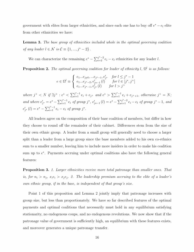
Lemma 3. The base group of ethnicities included whole in the optimal governing coalition

of any leader l ∈ N is C ≡ 1, ..., j∗ − 2 .

We can characterize the remaining e∗ −∑j∗−2

i=2 ei − el ethnicities for any leader l.

Proposition 2. The optimal governing coalition for leader of ethnicity l, Ωl is as follows:

e ∈ Ωl ≡

e1...ej 6=l, ...ej∗−1, e

′j∗ for l ≤ j∗ − 1

e1...ej∗−2, e′j∗−1 (l) for l ∈ [j∗, j+]

e1...ej∗−1, e′j∗ (l) for l > j+

where j+ < N if ∃j+ : e∗ <∑j∗−1

i=1 ei + ej+ and e∗ >∑j∗−1

i=1 ei + ej++1, otherwise j+ = N ;

and where e′j∗ = e∗−∑j∗−1

i=1 ei of group j∗, e′j∗−1 (l) = e∗−∑j∗−2

i=1 ei− el of group j∗− 1, and

e′j∗ (l) = e∗ −∑j∗−1

i=1 ei − el of group j∗.

All leaders agree on the composition of their base coalition of members, but differ in how

they choose to round off the remainder of their cabinet. Differences stem from the size of

their own ethnic group. A leader from a small group will generally need to choose a larger

split than a leader from a large group since the base members added to his own co-ethnics

sum to a smaller number, leaving him to include more insiders in order to make his coalition

sum up to e∗. Payments accruing under optimal coalitions also have the following general

features:

Proposition 3. 1. Larger ethnicities receive more total patronage than smaller ones. That

is, for ni > nj, xiei > xjej. 2. The leadership premium accruing to the elite of a leader’s

own ethnic group, if in the base, is independent of that group’s size.

Point 1 of this proposition and Lemma 2 jointly imply that patronage increases with

group size, but less than proportionately. We have so far described features of the optimal

payments and optimal coalitions that necessarily must hold in any equilibrium satisfying

stationarity, no endogenous coups, and no endogenous revolutions. We now show that if the

patronage value of government is sufficiently high, an equilibrium with these features exists,

and moreover generates a unique patronage transfer.

16

Proposition 4. Provided the patronage value of government is sufficiently high, the patron-

age transfers just sufficient to dissuade members of each ethnic elite from mounting a coup;

i.e. xj for j ∈ [1, j∗ − 1] are:

xjej =γ[1− xj∗e′j∗ −

γF1−γΣj∗−1

i=1 ei

]1 + γ(j∗ − 2)

+γF

1− γej,

where

xj∗e′j∗ =

1−e′j∗ej∗

γ2(j∗ − 2 +e′j∗−1

ej∗−1)

1 + γ(j∗ − 2)

−1

×

γ

1− (j∗ − 2 +e′j∗−1

ej∗−1

)γ[1− γF

1−γΣj∗−1i=1 ei

]1 + γ(j∗ − 2)

− γF

1− γ(Σj∗−2i=1 ei + e′j∗−1

) e′j∗ej∗

+ e′j∗F

,

and

e′j∗ = λP

(1− r −

j∗−2∑i=1

ni/P − nj∗−1/P

), e′j∗−1 = λP

(1− r −

j∗−2∑i=1

ni/P − nj∗/P

).

These leaders’ coalitions, and supporting transfers are the unique sub-game perfect sta-

tionary equilibrium of the model in which there are no endogenous coups or revolutions.

It is now also possible to explicitly specify the value function V transitionj defined in equation

(7), details of which we leave to the Appendix. The characterization of the uniquely optimal

coalition for each leader and of the patronage shares are both features extremely valuable to

the structural estimation of the model, to which we now proceed.

3 Econometric Specification and Estimation

To operationalize the solution in Proposition 4 additional assumptions are necessary. We

assume that the allocated shares of patronage are only partially observable due to a group-

specific error νjt. We imperfectly observe xie′i (l)i∈Ωl , the vector of the shares of patronage

allocated to ethnic groups in the ruling coalition (and consequently we also imperfectly

observe the leader group’s share xlel). Every player in the game observes such shares exactly,

but not the econometrician. For excluded groups j /∈ Ωl and j 6= l we also assume the

possibility of error to occur. For instance, consider the case of erroneously assigning a

minister to an ethnic group that is actually excluded from the ruling coalition.

17

At time t, let us indicate xjt = xj if j ∈ Ωl and xjt = 0 if j /∈ Ωl and j 6= l. Note

that the time dimension in xjt arises from the identity of the leader l shifting over time due

to transitions, as per Proposition 2. We define the latent variable X∗jt = xjte′j (l) + νjt and

specify:

(11) Xjt =

X∗jt if X∗jt ≥ 00 if X∗jt < 0

where Xjt indicates the realized cabinet post shares to group j ∈ N , hence Xjt ∈ [0, 1] with

allocation vector Xt= X1t,..., XNt. Note that (11) ignores right-censoring for X∗jt ≥ 1, as

Xjt = 1 never occurs in the data.

The error term ν is assumed mean zero and identically distributed across time and

ethnic groups. The distribution of ν with density function β(.) and cumulative function

B(.) is limited to a bounded support [−1, 1] and ν ∼ Beta (−1, 1, ξ, ξ) with identical shape

parameters ξ, a particularly suited distribution function18.

As noted in Adachi and Watanabe (2007), the condition Σi∈NXit = 1 can induce ν to

be dependently distributed across groups. Generally, independence of the vector νiti∈N is

preserved since Σi∈NXit = 1 6= Σi∈NX∗it due to censoring, but not for all realizations of the

random shock vector νiti∈N . To see this, notice that if all the observations happen to be

uncensored, then Σi∈NXit = Σi∈NX∗it = 1, implying that Σiνit = 0, which would give to the

vector νiti∈N a correlation of −1. In this instance we would only have N − 1 independent

draws of ν but N equations. A solution to this problem is to systematically employ only

N − 1 independent equations for each observed cabinet. Conservatively, we always exclude

the smallest group’s (N) share equation from estimation.

Absent any information on λ, the model can still be estimated and one is able to identify

the product λPF (but not λ and F separately). We follow this approach, set in the estimation

λP = 1, and rescale F when we discuss our results19. We also calibrate δ = .95.

Given the vector of model parameters θ = (γ, F, r, ξ, α, ε), conditional on the vector of

18For a discussion see Merlo (1997), Diermeier, Eraslan, and Merlo (2003), and Adachi and Watanabe(2007).

19Although systematic studies of African elites are rare, survey evidence in Kotze and Steyn (2003) in-dicates λ to be possibly approximated by population shares of individuals with tertiary education in thecountry. Any bias introduced by employing tertiary education shares as proxies for λ can be, in theory,assessed by comparing estimates of the other parameters of interest relative to our baseline which operateswithout any assumption on the size of λ. For space limitations we do not explore this avenue here.

18

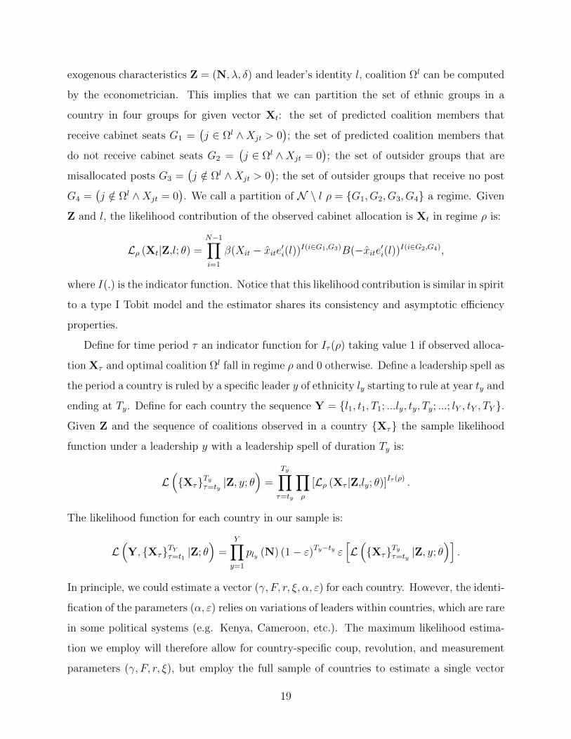
exogenous characteristics Z = (N, λ, δ) and leader’s identity l, coalition Ωl can be computed

by the econometrician. This implies that we can partition the set of ethnic groups in a

country in four groups for given vector Xt: the set of predicted coalition members that

receive cabinet seats G1 =(j ∈ Ωl ∧Xjt > 0

); the set of predicted coalition members that

do not receive cabinet seats G2 =(j ∈ Ωl ∧Xjt = 0

); the set of outsider groups that are

misallocated posts G3 =(j /∈ Ωl ∧Xjt > 0

); the set of outsider groups that receive no post

G4 =(j /∈ Ωl ∧Xjt = 0

). We call a partition of N \ l ρ = G1, G2, G3, G4 a regime. Given

Z and l, the likelihood contribution of the observed cabinet allocation is Xt in regime ρ is:

Lρ (Xt|Z,l; θ) =N−1∏i=1

β(Xit − xite′i(l))I(i∈G1,G3)B(−xite′i(l))I(i∈G2,G4),

where I(.) is the indicator function. Notice that this likelihood contribution is similar in spirit

to a type I Tobit model and the estimator shares its consistency and asymptotic efficiency

properties.

Define for time period τ an indicator function for Iτ (ρ) taking value 1 if observed alloca-

tion Xτ and optimal coalition Ωl fall in regime ρ and 0 otherwise. Define a leadership spell as

the period a country is ruled by a specific leader y of ethnicity ly starting to rule at year ty and

ending at Ty. Define for each country the sequence Y = l1, t1, T1; ...ly, ty, Ty; ...; lY , tY , TY .

Given Z and the sequence of coalitions observed in a country Xτ the sample likelihood

function under a leadership y with a leadership spell of duration Ty is:

L(XτTyτ=ty

|Z, y; θ)

=

Ty∏τ=ty

∏ρ

[Lρ (Xτ |Z,ly; θ)]Iτ (ρ) .

The likelihood function for each country in our sample is:

L(Y, XτTYτ=t1

|Z; θ)

=Y∏y=1

ply (N) (1− ε)Ty−ty ε[L(XτTyτ=ty

|Z, y; θ)]

.

In principle, we could estimate a vector (γ, F, r, ξ, α, ε) for each country. However, the identi-

fication of the parameters (α, ε) relies on variations of leaders within countries, which are rare

in some political systems (e.g. Kenya, Cameroon, etc.). The maximum likelihood estima-

tion we employ will therefore allow for country-specific coup, revolution, and measurement

parameters (γ, F, r, ξ), but employ the full sample of countries to estimate a single vector

19

Carlo simulations. For given parameter values we simulated country histories and made sure

the estimation based on the simulated data converged on the original structural values.

Given the parsimony of our model, the likelihood function depends on a relatively small

number of parameters. This allows for a fairly extensive search for global optima over the

parametric space. In particular, we first employ a genetic algorithm (GA) global optimizer

with a large initial population of 10, 000 values and then employ a simplex search method

using the GA values as initial values for the local optimizer. This approach combines the

global properties of the GA optimizer with the proven theoretical convergence properties of

the simplex method. Repeating the optimization procedure consistently delivers identical

global optima.

4 Data and Descriptive Statistics

In order to operationalize the allocation of patronage shares we rely on data on the

ethnicity of each cabinet member for fifteen African countries, sampled at yearly frequency

from independence to 2004. The full data description and the construction of ethnicity and

ministerial data, as well as evidence in support of the importance of this executive branch

data, is available in Rainer and Trebbi (2011). Here we will illustrate briefly the process of

data collection for each country. We devised a protocol involving four stages.

First, we recorded the names and positions of all government members that appear in the

annual publications of Africa South of the Sahara or The Europa World Year Book between

1960 and 2004. Although their official titles vary, for simplicity we refer to all the cabinet

members as “ministers” in what follows.

Second, for each minister on our list, we searched the World Biographical Information

System (WBIS) database for explicit information on his/her ethnicity. Whenever we could

not find explicit information on the minister’s ethnicity, we recorded his or her place of birth

and any additional information that could shed light on his/her ethnic or regional origin (e.g.,

the cities or regions in which he or she was politically active, ethnic or regional organizations

he/she was a member of, languages spoken, ethnic groups he/she wrote about, etc.).

Third, for each minister whose ethnicity was not found in the WBIS database, we con-

ducted an online search in Google.com, Google books, and Google Scholar. Again, we pri-

20

marily looked for explicit information on the minister’s ethnicity, but also collected data on

his/her place of birth and other information that may indicate ethnic affiliation. In addition

to the online searching, we sometimes also employed country-specific library materials, local

experts (mostly former African politicians and journalists with political expertise), and the

LexisNexis online database as alternative data sources.

Fourth, we created a complete list of the country’s ethnic groups based on ethnic cat-

egories listed by Alesina, et al. (2003) and Fearon (2003), and attempted to assign every

minister to one of these groups using the data collected in the second and third stages. When

our sources explicitly mentioned the minister’s ethnicity, we simply matched that ethnicity

to one of the ethnic groups on our list. Even when the explicit information on the minister’s

ethnicity was missing, we could often assign the minister to an ethnic group based on his or

her place of birth or other available information. Whenever we lacked sufficient evidence to

determine the minister’s ethnic group after this procedure, we coded it as “missing”. The

exact ethnic mappings are available in Rainer and Trebbi (2011).

This paper employs completed data since independence from colonization on Benin,

Cameroon, Cote d’Ivoire, Democratic Republic of Congo, Gabon, Ghana, Guinea, Liberia,

Nigeria, Republic of Congo, Sierra Leone, Tanzania, Togo, Kenya, and Uganda. In these

countries we were able to identify the ethnic group of more than 90 percent of the ministers

between 1960 and 2004. Our cross-sectional sample size exceeds that of most studies in

government coalition bargaining for parliamentary democracies.20

Table 1 presents the basic summary statistics by country for our sample, while Table 2

presents summary statistics further disaggregated at the ethnic group level.

4.1 Stylized Facts

An informative descriptive statistic is the share of the population not represented in the

cabinet for our African sample. Table 3 reports country averages. African ruling coalitions

are often in the 80 percent range. Just as comparison, in parliamentary democracies typically

only 50 percent of the voters find their party represented in the cabinet due to simple

20See for instance Diermeier, Eraslan, and Merlo (2003) and Ansolabehere, Snyder, Strauss, and Ting(2005).

21

majoritarian incentives (arguably not the relevant dimension for African autocracies). Given

no ethnic group in our sample represents more than 39 percent of the population, and in

no country in our sample does any leader’s group represent more than 30 percent of the

population, Table 3 implies that at least some members of non-leader ethnic groups are

always brought into the cabinet.

To further illustrate this feature, Table 4 reports a reduced-form specification with c

indicating a specific country, j the ethnic group, and t the year of the likelihood of inclusion

in a coalition:

Mcjt = αM1njcPc

+ γMc + δMt + ηMcjt

and with Mcjt indicator for ethnicity j at time t belonging to the cabinet. In a Probit

specification in Column (1), the marginal effect on the ethnic group share of the population,

αM1 , is positive and statistically significant. An extra 1 percent increase in the share of

the population of a group increases its likelihood of inclusion by 6.6%. This underlines a

strong relationship between size and inclusion in government. It is easy to see why. 94.5%

of all group-year observations representing 10% of the population or more hold at least one

position. 83.7% of those with 5% population or more hold at least one position. Column

(2) adds a control for the party/group being the largest in terms of size, in order to capture

additional nonlinearities, with similar results. Repeating the same exercise, but with respect

to the likelihood of a group holding the leadership, reveals an important role for size as well.

Table 4 Column (3) reports a marginal effect on the likelihood of leadership of .54 percent

per extra 1 percent increase in the share of the population of a group. This stylized fact

supports our assumption in (1).

We can also assess the overall degree of proportionality of African cabinets. The issue

of disproportionality is the subject of a substantial literature in political economics and

political science as a feature of electoral rules.21 Some Africanists have discussed the issue

of cabinet disproportionality in detail (Posner, 2005), emphasizing how for countries with

few reliable elections, cabinet disproportionality might be a revealing statistic. Recalling

that Xj indicates the realized cabinet post shares to group j, a first operational concept is

21In particular seat-votes differences. Gallagher (1991) explores the issue in detail and Carey and Hix(2011) offer a recent discussion.

22

the degree of proportionality of the cabinet. A perfectly proportionally apportioned cabinet

is one for which for every j ∈ N , nj/P = Xj. Governments, particularly in autocracies,

are considered to operate under substantial overweighting (nj/P < Xj) of certain factions

and underweighting (nj/P > Xj) of other ethnic groups. As discussed in Gallagher (1991),

deviations from proportionality can be differentially weighted, with more weight given to

large deviations than small ones or focusing on relative versus absolute deviations. Following

Gallagher, we focus on his preferred measure of disproportionality, the least squares measure

πLSqt =√

12

∑Ni=1 (100 ∗ (Xit − ni/P ))2.

We report the time series for πLSq for each country in Figure 1. The average levels of

disproportionality for the elites in each country are reported in Table 3, with larger values

indicating less proportionality and an average level of 16.72. As a reference, using party vote

shares and party cabinet post shares in the sample of democracies of Ansolabehere et al.

(2005) πLSq = 33.97 on average. Notice that πLSq captures well-known features of the data,

for example, the political monopoly of the Liberian-American minority in Liberia until the

1980’s. Overall, African cabinet allocations tend to closely match population shares with

cabinet seat shares, and disproportionality is low.

To further illustrate this feature, Table 5 reports a straightforward reduced-form regres-

sion of cabinet shares on population shares:

Xcjt = αX1njcPc

+ αX2 Lcjt + γXc + δXt + ηXcjt

with Lcjt an indicator function for the country leader belonging to ethnicity j at time t.

Lcjt captures the straightforward nonlinearity stemming from leadership premia. Column

(1) in Table 5 shows two striking features. First, the coefficient on the ethnic group share

of the population αX1 is positive and statistically significant, indicating a non trivial degree

of proportionality between population shares and cabinet allocations, around .77. This

rejects clearly the hypothesis of cabinet posts being allocated independently of the population

strength of a group and at the whim of the leader and verifies point 1 of Proposition (3).

Second, the leader’s seat premium in the cabinet is precisely estimated, positive, but not

excessively large: around 11 percent. Given an average cabinet size of 25 posts in our African

sample, the leadership premium can be assessed as an additional 1.75 = 25 ∗ (0.11 − 1/25)

23

ministerial positions on top of the leadership itself.

A more subtle implication of our model is the combination of Proposition (3) and Lemma

(2), as for two non-leader groups j and k, if ej > ek, then xjej < xkek but xj < xk.

Column (2) includes the square of the group size to capture the reduction in representation

for larger groups. The coefficient on (njc/Pc)2 is negative and statistically precise. This

reduced-form finding supports the view of larger groups gaining seats but being relatively

less well represented than smaller ones; the specific type of nonlinearity implied by Lemma

(2). In Column (3) we restrict the analysis to non-leader ethnicities, with more precise

estimates. Figure 2 gives a graphical representation of this result fitting a nonparametric

lowess of cabinet shares as function of population shares, pooled across countries and non-

leader ethnicities. Note that the bandwidth of the lowess is 0.8, so the curvature at the

upper extreme of the graph is not driven by a few large observations, but estimated using

groups as low as 0.04. Overall, the concavity of the reduced-form relationship is a validation

of this specific aspect of our model.

The allocation of top positions in African cabinets is explored in Column (4) of Table

5. We include as top ministerial posts: the Presidency/Premiership, Defense, Budget, Com-

merce, Finance, Treasury, Economy, Agriculture, Justice, Foreign Affairs. Both size and

leadership status are positive and significant. Quantitatively, it is surprising that αX1 re-

mains sizable in Column (4), close to that estimated in Column (1). Notice also how the

effect of leadership increases for top ministerial appointments, this is however the result of

the leader representing a larger share of a smaller set of posts. Given an average top cabinet

size of 9 posts, the leadership premium can be assessed as an additional 0.87 = 9∗(.208−1/9)

ministerial positions on top of the leadership itself.

Not only do African cabinet allocations tend to mirror population shares closely, but they

do so consistently over time. As an illustration, we report the time series of (Xit − ni/P )

across all ethnic groups in Guinea (Figure 3) and in Kenya (Figure 4)22. The time series

hover around zero, unless the leader is from that specific ethnicity (in which case there is a

positive gap). As predicted by our model, there appear to be leadership premia. In Guinea

the shift in power between Malinke and Susu in 1984 at the death of Ahmed Sekou Toure,

22Similar patterns recur across the other countries.

24

a Malinke, produced a visible drop in overweighting of that group and a jump for the Susu,

the new leader’s group. Similar dynamics are evident under Moi in Kenya. Overall, these

stylized facts strongly justify our focus on stationary equilibria.

5 Results

5.1 MLE Results

Table 6 presents our maximum likelihood estimates of the model. We report the full vec-

tor of model parameters θ = (α, ε, γ,F, r, ξ) where we use the notation γ =(γBEN , γCMR, ..., γUGA

),

F =(FBEN , FCMR, ..., FUGA

), and so on, for country-specific parameters.

Beginning from the common parameters governing the leadership transitions, we find

immediate support for the view that larger groups are more likely to produce leaders, i.e.

α > 0. In addition, α is precisely estimated at 11.5 > exp(1), implying that large groups are

substantially overweighted relative to small groups. This finding highlights increasing returns

to scale in terms of likelihood of leadership appointment for ethnic groups. If it were possible,

different ethnic groups could gain in terms of likelihood of generating a leader by merging.

Regarding the likelihood of exogenous breakdowns in power, inclusive of uninsurable coups

or other shocks, we estimate an ε around 11.5%, again very statistically significant23 This

indicates a fairly high likelihood of per-period breakdown and translates into an effective per

period discount rate24 of δ(1− ε) = .95 ∗ .905 = 84%.

Concerning the country-specific parameters, let us begin from the revolution technology

parameter r, where 1−r is the share of value destroyed by the revolution. For virtually every

country, r is precisely estimated. In a fashion completely consistent with the large ruling

coalitions highlighted in Figure 1, Table 6 reports values of r generally above 80%. Larger

values of r imply cheaper, less destructive revolutions. Cheaper revolutions, in turn, imply

larger threats to the leader from outsiders, pushing him toward more inclusive governments.

It is not surprising, then, that we estimate r = 0.99 for Guinea, a country with average

23Note also that our assumption about i.i.d. ε transitions is valid. A diagnostic Breusch and Pagan(1980) LM test for cross-country dependence of ε cannot reject independence with a p-value of .84 and anArellano-Bond panel model of a leader transition on its lag cannot reject serial independence with a p-valueof .95.

24It should also be clear from this calculation why we calibrate δ = .95, as it cannot be separately identifiedfrom ε.

25

observed coalitions around 92% of the population (the highest of all 15 countries). There are

only 9 ethnicities in Guinea and the top 7 by size all have nontrivial observed cabinet shares,

while the bottom two groups are only 1% of the population each. So, one could imagine the

estimator trying to include at least the top 7.

The precision parameter ξ governing the Beta distribution of the error terms is generally

quite high. Larger values of ξ imply tighter distributions of the ν’s in (11) and underline

a good fit of the model (further explored below). The country with the lowest precision is

Liberia, with a fit ξ = 24.5.

Indeed Liberia requires a short diversion. One can recall that the stylized facts reported in

Figure 1 present Liberia as a clear outlier during the 1960-1980 period; a period of American-

Liberian rule. During the Americo-Liberian era, the country was essentially ruled by a small

minority of freed American slaves repatriated to this particular area since the 1820s under

the auspices of the United States government. On average the Americo-Liberian regime

concentrated around 50% of cabinet seats into a 4% population minority. The international

economic and political support for the Americo-Liberians sustained their central rule, but

waned over time. With a coup ending the regime in 1980. The Americo-Liberian period

clearly clashes with our model’s assumptions as we are ignoring the vast military-economic

advantage and international support with which the Americo-Liberians were endowed. We

consider Liberia in much of the discussion below as a useful falsification case.

The coup technology parameter, γ, and the private returns to leadership F (expressed

as share of total transferable patronage) are of particular interest for understanding the

allocation of seats. Increasing γ for given F makes coups more threatening for a leader

because of their higher success rate, and induces a more proportional allocation of government

posts. Increasing F for given γ makes coups more threatening for a leader as well, because

of the higher value of taking over if the coup is successful, and this again induces a more

proportional allocation of posts in order to avoid coups. Both parameters are generally

precisely estimated in Table 6. For Benin, Cameroon, and Gabon the model does not pin

down γ and F precisely, pushing γ toward a corner of 0 and F toward very large valuations.

Uganda instead displays an imprecise, low γ. As we will show below, the model fit for these

countries is not particularly poor even though estimates do not allow us to precisely assess

26

the role of γ and F independently. Only Liberia, and for the reasons stated before, seems to

reject the model.

Averaging the estimates of γ in the ten countries for which we have interior estimates and

excluding Liberia, one can notice the importance of the coup threat in driving the allocation

of cabinet posts. The average likelihood of coup success γ is fairly large, about 35%. The

quantitative interpretation of the reported F , which averages at 2.5, is harder. First of all,

we need to scale by λP the estimates of F reported in Table 6. This delivers private rents to

the leader as a share of total value of patronage in the country. Using as benchmark for the

elite share of the population 1/1000 gives us a scaling factor 1/λP = (.001∗P )−1. Averaging

the estimates of the rescaled F , implies that yearly private rents as share of total patronage

allocated in a country of 20 million people are around 2.5/(.001 ∗ 20M), probably not an

unrealistic figure when multiplied by total value of government patronage in the country.25

Table 7 reports two additional statistics and their standard errors. First we compute the

structural slope of cabinet allocations as function of size of the ethnic group γF/(1 − γ).

These estimates are positive and statistically significant with the exception of Liberia, which

is negative, implying over-representation of small groups (an unsurprising fact given the

pre-1980 era). Positive slopes imply that a larger group size predicts a larger share of posts

(and patronage), as implied by point 1 of Proposition (3). For the ten countries for which

we have interior estimates of γ and F and excluding Liberia, the slope is also statistically

smaller than 1 implying under-representation of non-leader groups and positive leadership

premia, which we verify in the second column of Table 7. For Benin, Cameroon, Gabon,

and Uganda point 1 of Proposition (3) is also verified, as the estimated slope is positive and

significant. Concerning the estimated leadership premia accruing to a member of the base

coalition, typically the estimates are precise and positive, consistent with our theoretical

setup. We find average leadership premia across our countries around 9− 12 percent share

of the cabinet seats. Notice also that a leadership premium of about 12 percent is a figure

similar to that which was estimated in Section 3 in the reduced-form relationship.

25As an hypothetical benchmark one can consider a country with a GDP of $30 Billion and governmentspending/GDP of 30% (similar to current Kenya or Cameroon in our sample). This would deliver yearlyprivate rents from office around $1.4 million. Such estimates, however, have to be considered with extremecaution, as it is particularly complex to exactly quantify the absolute size of both ethnic elites and governmentpatronage.

27

An important check comes from the analysis of top cabinet positions, like defense or

finance. Our results are not just an artifact of the leadership allocating minor cabinet roles

to ethnicities different from the leader’s own. The results hold true even when restricting the

analysis to the subsample of the most powerful ministerial posts. In Tables 8-9 we report

ML estimates for a model that gives weight 1 to the top posts and 0 to all other cabinet

appointments. Proportionality and leadership premia appear remarkably stable across the

top position model and the full sample model, although the estimated precision parameters

ξ governing the Beta distribution are now lower, a natural consequence of the coarser nature

of the allocated top shares. Given the precision of our ML estimates, we can typically reject

equality of the estimates across the two models, but the magnitudes appear economically

similar. Given the crucial strategic role of some of these cabinet positions within autocratic

regimes (e.g. ministry of defense), it appears natural to infer that some real power is actually

allocated from the leadership to other ethnic factions.

Finally, in Appendix Table A1 we report the results for the full model under the more

general revolution contest function (Σi∈NOn

χi

Σi∈NOnχi +Σi∈NIn

χi), which nests our specification and al-

lows for ethnic fractionalization within contesting groups in a revolution to alter effectiveness

due to coordination costs χ. The baseline model in Table 6 imposes χ = 1, while Table A1

shows that a model with a χ slightly below 1 fits the data better in a majority of countries.

This suggests another reason for leaders to prefer elites from larger groups in their governing

coalitions – in addition to their being ‘cheaper’ via the model’s coup constraint. A positive

χ value lower than 1 implies that reducing fractionalization increases the effectiveness of

given government forces in the contest function. The other parameter estimates are largely

unaltered and we focus on the simpler χ = 1 specification from here on.

5.2 In-Sample and Out-of-Sample Goodness of Fit

Our model predicts that ruling coalitions should include first and foremost large groups,

that the share allocated to such groups should be stable over time, and that cabinet posts

should be allocated proportionally to group size but at diminishing rates. Failing to match

any of these moments in the data will deliver poor fit of the model. We now illustrate the

28

goodness of fit of our model by focusing on a set of characteristics of African coalitions.26

In Sample

We begin by checking the in-sample fit over the entire 1960-2004 period using the esti-

mates of Table 6 and the implied optimal coalitions. Figure 5 reports the observed coalition

sizes in terms of share of population represented by each group in government. This means

that an observed average coalition of .7 in Ghana indicates that summing up the ethnic

shares of the population of every ethnicity with at least one minister covers 70% of the pop-

ulation on average each year over the 1960-2004 period. Our model predicts a very similar

coalition size, about 73%. With the exception of Liberia and Tanzania our model fares very

well in predicting the size of the coalitions as fractions of the population. On average we are

able to correctly predict around 80% of the population based on the assignment to govern-

ment insiders or outsiders, as reported in Figure 6. This means that our model accurately

predicts the membership of the cabinet in terms of relevant groups in the population. Even

considering simple counts of groups correctly predicted in or out of government, i.e. equally

weighing very large and very tiny ethnicities, we observe a high success rate, often correctly

assigning more than 2/3 of the ethnic groups in our sample. Excluding Liberia, the observed

coalitions cover on average 79.4% of the population based on ministerial ethnic affiliations,

while our in-sample prediction is 84.4%.

Concerning how we fit government shares, and not just government participation, it

would be cumbersome to report shares for every ethnicity across 15 countries. Instead, we

focus on two specific typologies of groups which are of paramount relevance. We fit the

cabinet shares of the ethnic group of the leader in Figure 7 and the cabinet shares of the

largest ethnic group in the country in Figure 8. These two ethnic groups do not overlap

substantially (78% of the leader’s group observations are not from the largest ethnicity).

Once again, inspection of the figures reveals a very good match of the theoretical allocations

and the allocations observed in the data. Excluding Liberia, observed cabinet post shares

to leaders are 20.2% on average, while our model predicts 22%. Excluding Liberia, observed

26In the appendix we also report the fit obtained under a generalization of the model that allows frac-tionalization to influence the effectiveness of coalitions under the contest function. That model embeds thelinear contest functions here as a special case, and by allowing non-linearities, does an even better job inmatching characteristics of the data.

29

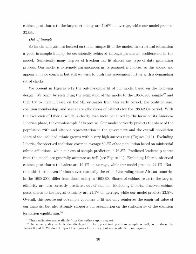
cabinet post shares to the largest ethnicity are 21.6% on average, while our model predicts

23.8%.

Out of Sample

So far the analysis has focused on the in-sample fit of the model. In structural estimation

a good in-sample fit may be occasionally achieved through parameter proliferation in the

model. Sufficiently many degrees of freedom can fit almost any type of data generating

process. Our model is extremely parsimonious in its parametric choices, so this should not

appear a major concern, but still we wish to push this assessment further with a demanding

set of checks.

We present in Figures 9-12 the out-of-sample fit of our model based on the following

design. We begin by restricting the estimation of the model to the 1960-1980 sample27 and

then try to match, based on the ML estimates from this early period, the coalition size,

coalition membership, and seat share allocations of cabinets for the 1980-2004 period. With

the exception of Liberia, which is clearly even more penalized by the focus on its Americo-

Liberian phase, the out-of-sample fit is precise. Our model correctly predicts the share of the

population with and without representation in the government and the overall population

share of the included ethnic groups with a very high success rate (Figures 9-10). Excluding

Liberia, the observed coalitions cover on average 82.5% of the population based on ministerial

ethnic affiliations, while our out-of-sample prediction is 76.3%. Predicted leadership shares

from the model are generally accurate as well (see Figure 11). Excluding Liberia, observed

cabinet post shares to leaders are 19.1% on average, while our model predicts 24.1%. Note

that this is true even if almost systematically the ethnicities ruling these African countries

in the 1980-2004 differ from those ruling in 1960-80. Shares of cabinet seats to the largest

ethnicity are also correctly predicted out of sample. Excluding Liberia, observed cabinet

posts shares to the largest ethnicity are 21.1% on average, while our model predicts 23.5%.

Overall, this precise out-of-sample goodness of fit not only reinforces the empirical value of

our analysis, but also strongly supports our assumption on the stationarity of the coalition

formation equilibrium.28

27These estimates are available from the authors upon request.28The same quality of fit is also displayed in the top cabinet positions sample as well, as produced by

Tables 8 and 9. We do not report the figures for brevity, but are available upon request.

30

5.3 Fit Along Additional Dimensions

By considering the relative fit of the model over different subsamples, some of the country

institutional and political details, deliberately omitted from the model, can be assessed. Were

the model missing relevant institutional dimensions, the fit would drastically deteriorate in

that specific subsample.

Informally, we can observe in Table 6 that fit and precision of our estimates are consistent

across English and French colonial origin countries and East and West African countries. Our

model seems to capture allocation mechanisms of historically different regimes, occasionally

even delivering quantitatively similar outcomes (e.g. Guinea and Kenya in Table 6).

More formally, we can evaluate different subsamples separately, assessing whether the

main results are driven by any specific dimension of the data and whether the fit is con-

sistently accurate across samples. We chose two important dimensions: military nature of

the regime and form of government. For military versus civilian rule, about 58% of our

country-year observations fall in the latter category based on a classification that incorpo-

rates both Archigos and the Europa Year Book (Rainer and Trebbi, 2011). Military regimes

are often considered organizationally different than civilian structures, as more hierarchical

in nature. With regard to autocratic versus democratic forms of government, about 14% of

our country-year observations fall in the latter category based on the Polity2 score of the

country (we define a democracy as Polity2 score > 5, as standard in the literature). We

do not report the ML estimates for all the separate subsamples29, but only focus on the

predictions of our model for coalition size and leader group’s share.

The fit is consistently good across subsamples. For military regimes, the predicted average

coalition size pooling all countries and time periods is .83 versus an actual size of .78 and the

predicted leader’s share is .20 versus an actual share of .19. For civilian regimes, the predicted

average coalition size is .88 versus an actual size of .77, while the predicted leader’s share

is .26 versus an actual share of .24. For autocratic regimes, the predicted average coalition

size is .83 versus an actual size of .77, while the predicted leader’s share is .24 versus an

actual share of .22. For democratic periods, the predicted average coalition size is .77 versus

an actual size of .80, while the predicted leader’s share is .25 versus an actual share of

29All results available from the authors upon request.

31

.22. Surprisingly, even though there are few democratic regimes and our model is clearly

not apt to describe modern democratic power sharing, the model’s fit is still accurate. A

conjecture would be that democratic transitions do not completely make tabula rasa of the

power structure in place during autocratic periods.

6 Counterfactuals

We now investigate a set of counterfactual experiments based on our structural estimates.

Concerning the role of the revolution and coup technologies in the allocation of ministerial

posts in Africa, we focus on three counterfactuals: i) an increase in the cost of the revolution

parameter, 1− r; ii) a reduction in the likelihood of success of coups, γ; and iii) a reduction

of the size of the private benefits from leadership, F . Lowering r produces more exclusive

coalitions by increasing the cost of revolt against the leader and hence makes revolutions

less threatening. Drops in γ and F make coups less threatening for the leader as well. As

leadership becomes safer to maintain, lower γ and F induce a less proportional allocation of

seats relative to group size and more rents for the leader’s ethnic group. Large coalitions and

close-to-proportional patronage allocations are a result of the fragility of the institutional

structure of Sub-Saharan countries. As fourth counterfactual, we explore the effects of

counterfactual ethnic group distributions within countries. We show how an increase in

ethnic fractionalization translates into larger coalitions and seats losses to the leadership.

We begin by estimating the model for the 1960-1980 sample. We then modify only one

parameter at a time and observe how the model predictions change in the 1980-2004 sample.

One could potentially simulate the counterfactuals using the entire 1960-2004 sample as well.

We opt for the former approach in order to show how different the out-of-sample predictions

would be in presence of structural breaks in each of the main parameters of the model.

A. Reducing the Threat of Revolutions

Figures 13-15 present the counterfactual coalitions in presence of a 10% drop in r vis-a-

vis the baseline predicted coalition, shares allocated to leaders, and shares allocated to the

largest group. In Figure 13 the population share with at least one minister represented in

the coalition falls substantially when lowering r. The threat of revolutions is so reduced by

the increase in their cost that coalitions drop in size from 76.3% in the baseline to 48.3%

32

of the population in the counterfactual (on average across all countries, excluding Liberia).

Concerning allocated shares within these smaller coalitions, we notice that the leader’s groups

now enjoy substantially higher shares of cabinet seats, going from 24.1% to 56.2% on average

across all countries (Figure 14). In Figure 15 the largest group also gains seat shares, moving

from 23.5% to 37.8%.

B. Reducing the Threat of Coups

Figures 16-18 present the counterfactual coalitions and allocations in presence of a 25%

relative drop in γ. Similarly, Figures 19-21 present the same counterfactuals in presence of

a 25% relative reduction in F . Notice that changing γ and F does not necessarily affect the

optimal coalition unless the insider revolt constraint (4) starts binding. However, changing

γ and F always affects how much a member of the coalition is paid.

The difference between modifying the coup technology and modifying the revolution

technology is substantial. In both Figure 16 and Figure 19 we notice that even a drastic

drop in γ or F does not affect the optimal coalition, leaving the insider constraint (4) slack.

Insiders are paid less when they are less dangerous (as they have lower incentives to stage a

coup), but they do not appear to have incentive to abandon the ruling coalition and hence

the leader does not change the composition of Ωl. Counterfactual coalitions under the new

γ and F have the same membership as the baseline in Figures 16 and 19. Notice that this

is true even if in relative terms the drops in γ or F are much higher than the relative drop

in r we have considered above.

Reducing the threat of coups does have an effect on allocations within the coalition.

When reducing γ, the leader’s group gets to enjoy a higher seat share, going from 24.1% to

34% on average across all countries excluding Liberia (Figure 17). Interestingly, the largest

group is less of threat now and therefore the leader assures its loyalty more cheaply. In

Figure 18 the largest group loses seat shares, moving from 23.5% to 21.6% when γ drops.

In the counterfactual reducing F , the leader’s group again enjoys higher shares of seats, up

from 24.1% to 30% on average across all countries excluding Liberia (Figure 20). In Figure

21 the largest group again loses seat shares, moving down from 23.5% to 21.5%.

C. Increasing Ethnic Fractionalization

A standard index of ethnic fractionalization considered here is the Herfindahl concentra-

33

tion30 ELF = 1−ΣNi=1 (ni/P )2. Typically an increase in ELF will require a shift towards a

more equal distribution of population across groups. Insider groups, the large ones according

to our model, should lose clout vis-a-vis outsiders, which are typically small.31

As an example, let us impose a reduction of 1 percent of the population to any group

above the median group size, while adding 1 percent to any group below the median (the

median group is left unchanged). This modification essentially tilts the distribution towards

equal shares of 1/N , which maximizes ELF . It also unambiguously strengthens small groups

on the outside of the government and weakens government insiders. The endogenous response

predicted by our model is a more inclusive coalition, which is what we observe across the

board in the counterfactuals of Figure 22. The increase in ethnic fractionalization has the

effect of increasing the average coalition size from 75.5 percent of the population to 76.9

percent. Interestingly, both the allocations to the leader’s own group and to the largest

group in the country decrease in Figures 23-24. By reducing the inequality in group size,

an increase in ELF makes challengers to the leadership more threatening and induces more

redistribution of the leadership and insiders’ spoils. The average share to the leader’s group

across the countries in our sample drops from 25.9 to 24.1 percent, while the largest group’s

share drops from 22.3 to 20 percent. The latter is a more than proportional reduction given

the 1 percent fall in the largest group population shares.

7 Alternative Models of Allocation

We now assess the relative performance of our model versus two relevant alternative

hypotheses. A first model of allocation, which could challenge our theoretical interpretation,

is one of pure window dressing on the part of the leader. One could reasonably conjecture

a proportional mechanism of cabinet allocation simply based on random sampling from the

30See Alesina et al. (2003); Fearon (2003), but also Posner (2004) for a criticism and an alternativemeasure. For an analysis of the determinants of ethnolinguistic diversity see Michalopoulos (2012).

31This intuition is generally correct. However, the specific effect of ELF on post allocations needs to bestudied on an case-by-case basis within our framework. The reason is that there are multiple ways an ethnicgroup distribution N = n1,..., nN can be modified to increase ELF . Carefully shifting mass across groupsmay produce no change in the balance of strength between insiders and outsiders, while still increasing ELF .This ambiguity is the result of the large amount of degrees of freedom allowed when the full vector of groupsizes N is modified. The following example clarifies how our model captures distributional changes in astraightforward case.

34

population of elites. Were the leader only concerned with giving an appearance of fair

representation of ethnic interests, he could just pick political pawns at random (plus or

minus a statistical error ν). Censoring should be allowed in such alternative setup as well,

but only due to the coarseness of the cabinet allocation process (e.g. a group with 1/30

of the population can not be proportionally represented in a cabinet of 20 seats) and not

because of revolution constraints. Formally, this would imply:

xjtej = ej for any j

and latent shares equal to:

X∗jt = xjtej + νjt.

Although relying on somewhat arbitrary assumptions about the lack of rationality of non-

elites (systematically fooled by such window dressing), this alternative model would appear

a strong challenger to our baseline. It embeds an assumption of proportionality of seat

allocation and has the ability to accommodate censoring.

A second alternative model of allocation that we explore here is a strong version of

the “big man” autocratic model. We wish to reject starkly a pure interpretation of ethnic

favoritism on the part of the ruler, a winner-take-all specification of the form:

xjtej =

0 for any j 6= l1 for l

and latent shares equal to:

X∗jt = xjtej + νjt.

We already have a sense that such degree of disproportionality might be rejected by the data

in light of the evidence above. However, one should consider that the alternative models

presented here are much more parametrically parsimonious than the model of Section 2, by

45 parameters, a factor which weighs against our baseline in formal model selection tests.

Since all models are non-nested, a standard econometric approach is to run generalized

likelihood ratio tests of model selection. We employ both the Vuong (1989) and Clarke

(2003) model selection tests. The null hypothesis for both the Vuong and Clarke tests is

that the baseline and the alternative model are both true against a two-sided alternative

that only one of the two models is true. The former test has better power properties when

35

the density of the likelihood ratios of the baseline and the alternative is normal, while the

latter is a more powerful test when this condition is violated. The baseline specification is

always our main model from Table 6, and it is tested against the random allocation model,

first, and the “big man” model, next. Table 10 reports all test statistics and p-values.

Our model fares substantially better than the proposed alternatives according to the

Vuong test for non-nested models.32 The test statistic of the baseline against the random

allocation model is 19 and we reject the null of equivalent fit with a p value of < 0.001 based

on a difference of 45 degrees of freedom (r, F, γ for 15 countries)33. Our model appears closer

to the actual data generating process. The rejection of the the “big man” autocratic model

is even starker, with a test statistic of 60.1 in favor of the baseline. Employing the Clarke

(2003) test we reject the null of equal fit for the random coalition model with a p-value of 0.

We reject the null of equal fit for the “big man” model with a p-value of 0.0002. Interestingly

the “big man” model fares slightly better using the Clarke test, as the statistic is based on

the number of positive differences between individual loglikelihoods, independently on the

actual size of those differences.

Table 10 reports the Vuong and Clarke tests for four subsamples considered in Section 5.3

(military, civilian, autocracies, democracies). In all subsamples the baseline model trumps

both alternative models, indicating that our theoretical setup is not dominated by alternative

mechanisms that may be at work within these specific subsets. The only exception is the

case of democratic regimes for the random allocation model. Here we see that, although

the loglikelihood for the baseline model is higher than the loglikelihood for the random

allocation model, the tests reject the baseline in favor of the random model. The reason is

the relative lack of parsimony of the baseline model relative to the random model. Both

Vuong and Clarke statistics penalize lack of parsimony, especially with small samples like for

this case (only 722 out of 11749 group-country-year observations). Due to the small sample

of democratic regimes, we would not venture in asserting that democratic periods present

radical breaks from our baseline allocation model.

32In the appendix we show that the generalization of the model including non-linearities in the contestfunction fits better still.

33The Vuong test statistic is asymptotically distributed as a standard normal.

36

8 Conclusions

This paper presents a model of the allocation of power within African polities and esti-

mates it employing a novel data set of the ethnic composition of African ministerial cabinets

since independence. Our data offer new insight into the internal mechanics of autocracies,

otherwise particularly opaque government forms, and their diverse upper echelons.

The data reject strongly the view of African autocracies as being run as “one man shows”

by a single leader and his ethnic group, with the sole exception of Liberia. The data display

inclusive coalitions and a positive and highly statistically significant degree of proportionality

of ministerial positions to ethnic group size in the population, suggesting a substantial degree

of political bargaining occurring within these polities. These findings are confirmed when

limiting the analysis to top cabinet posts alone.

Through the lens of our model these empirical regularities conform to a view of large

threats from revolutions and internal coups, which push African leaders towards inclusive-

ness. Our parsimonious model displays an excellent fit of the data in and out of sample

and can be considered a useful stepping stone for the analysis of African politico-economic

dynamics. We also perform new counterfactual experiments by modifying the revolution and

coup technologies in each country.

Future research should address the determinants of relative power among ethnic groups

besides sheer population size, the consequences of shocks to specific ethnic groups, including

climatic or terms of trade shocks to local resources, and should employ group-level informa-

tion for non-elites to further analyze the process of within-group political bargaining. In the

Appendix of this paper we extend our model to highlight the connection between within-

ethnic group frictions and between-ethnic group tensions that will also form the basis of

future work with this data. The data employed in this paper will also aid future research on

the internal organization of autocracies, especially with regard to the dynamics of ministerial

and inner circle turnover (Francois, Rainer, and Trebbi, 2012).

37

9 Appendix

9.1 Proofs

Proof of Lemma 1:Consider a hypothetical equilibrium that does not have a base coalition C. Denote the

equilibrium payments to elites of ethnicity j by xej in such an equilibrium. Moreover, assumethat xek = inf xe1..xeN and suppose this infimum is unique. Since there are no base ethnicitiesin this equilibrium, for any such ethnicity k, there exists at least one leader l 6= j whooptimally chooses not to include k in his governing coalition. But this implies that l cannotbe optimally choosing his coalition, as he is excluding support from the elite of an ethnicitywho will provide it at a price lower than those in his chosen coalition. So inf xe1..xeN beingunique is inconsistent with the non-existence of a base coalition.

It now remains to show what happens if inf xe1..xeN is not unique. There must now be atleast two infima, and denote these two k and j with xek = xej . Since there is no base coalition,there exists at least one leader l 6= k, j who optimally chooses not to include k and/or j inhis governing coalition. If not, either k or j would constitute a ‘base’ set of ethnicities C,violating the supposition. But for both k, j to not be included in all other leaders’ optimalcoalitions, i.e. for a base group of ethnicities not to exist, this must imply that there existsat least one more group m for whom xem = xej = xek. Without at least one alternative groupm, it would be impossible for leaders to not choose either k or j when choosing their optimalcoalition. Applying the same reasoning to group m, the only way that there cannot exista base group of ethnicities is if there exists a set of groups whose elites sum to a numberstrictly larger than e∗ in total and whose equilibrium xe values are all equal to the lowestequilibrium payment inf xe1..xeN . Without this, different leaders would be forced to chooseat least some members of the same ethnicities when constructing optimal coalitions. Only ifthere exist an amount strictly greater than e∗ of ethnicities all equally receiving the lowestvalues of x can a leader from m choose an ethnicity not included in a leader from l′s optimalcoalition, so that a base coalition may not exist.

So it remains possible that the per-elite member cost of buying support is identical forall leaders, but comprised of differing sets of elite. Denote such per elite member costs xe.The total payment of patronage required to buy support is thus (e∗ − el)xe, for a leader of

ethnicity l, implying per period returns of 1−(e∗−el)xeel

+ F. But for this to be consistent with

equivalent values (xe) for each leader, necessarily for two leaders m and l, where m denotesthe larger of the two so that em = wel and w > 1, we have:

xe ≡ xl = γ

(1− (e∗ − el)xe

el+ F

)= γ

(1− (e∗ − em)xe

em+ F

)= xm ≡ xe

=⇒ 1− (e∗ − el)xe

el=

1− (e∗ − wel)xe

wel=⇒ (1− (e∗ − el)xe)w = 1− (e∗ − wel)xe

=⇒ w (1− e∗xe) = 1− e∗xe

=⇒ w = 1.

But this is a contradiction, so it is not possible that the amount required to buy support

38

of ethnicities of different sizes is equivalent. Given this, necessarily there must exist a basegroup of ethnicities included in all leaders’ coalitions.

Proof of Lemma 2: Consider the payments required for members of two distinct elites,j and k in the base group that are being bought off by the coalition being formed by a leaderfrom group l, denoted Ωl, and suppose that ej > ek. Using (9) and (2) and the fact that atmost there is a unique included ethnicity that will be split, these are given by:

xjej = γ(

1− Σi 6=k,i∈Ωjxiei − x′(j)e

′(j)− xkek + ejF

)(12)

xkek = γ(

1− Σi 6=j,i∈Ωkxiei − x′(k)e

′(k)− xjej + ekF

).

We explicitly denote the split group separately with a ′. Since both j and k are in the basecoalition they both have identically comprised governing coalitions: when a j is leader, allelites from k are included and paid xk when a k is leader, all elites from j are included and paidxj. This implies that for the remainder, there is equivalence: Σi 6=k,i∈Ωjxiei = Σi 6=j,i∈Ωkxiei.Also both types of leader will have identically sized split groups, comprising the cheapest non-base elites available so that x

′(j)e

′(j) = x

′(k)e

′(k). Consequently, subtracting the second

from the first equation above leaves:

xjej − xkek = γ (xjej − xkek) + (ej − ek) γF

∴(xjej − xkek)

(ej − ek)=

γF

(1− γ).(13)

Let w > 1 denote the ratio of elite sizes, j and k so that ej = wek. Rewriting (13) using thisnotation yields:

wxj − xkw − 1

=γF

(1− γ)

∴ xk = wxj +(1− w) γF

(1− γ).(14)

To prove the claim it is necessary to show that since ej > ek necessarily xk > xj. Using (14),xk > xj if and only if:

wxj +(1− w) γF

(1− γ)> xj

xj >γF

(1− γ)

or γxj < xj − γF .

But we know from (12) that,

xj − γF =γ(1− Σi 6=k,i∈Ωjxiei − x′(j)e′(j)− xkek

)ej

≡ γxj.

39

So we need to show that:

γxj < γxj

⇔xj < xj.

Since we only consider equilibria without coups or revolutions, a necessary condition is thatelite from any governing ethnicity, including the leader’s own, have no incentive to mount acoup. Thus, necessarily for an equilibrium of this form to exist xj < xj, we ignore the zeromeasure parameter configuration where the residual left after paying off all other ethnicitiesjust equals the incentive compatible amount for co-ethnics (i.e., ignoring xjej = xjej). Ifthis condition were violated leader j′s co-ethnic elite would have incentive to mount a coup.Which thus proves the claim.

Proof of Proposition 1: Since any candidate equilibrium has payments determined by(9) we know that, for an elite of group j the payment is xj = γ

((1− Σi∈Ωjxiei − x

′(j)e

′(j))/ej + F

)and for elite j + 1 it is xj+1 = γ

((1− Σi∈Ωj+1xiei − x

′(j + 1)e

′(j + 1)

)/ej+1 + F

). The dif-

ference xj − xj+1 can be expressed as:

γ((

1− Σi∈Ωjxiei − x′(j)e

′(j))/ej + F

)− γ

((1− Σi∈Ωj+1xiei − x

′(j + 1)e

′(j + 1)

)/ej+1 + F

)≡ γ

ejej+1

[(1− Σi∈Ωjxiei − x

′(j)e

′(j))ej+1 −

(1− Σi∈Ωj+1xiei − x

′(j + 1)e

′(j + 1)

)ej

](15)

where x′(j + 1) is the per elite payment to the highest paid group for leader j + 1. Nownote that since ej > ej+1 a leader of ethnicity j+ 1 must buy the support of a strictly largernumber of elite than does a leader of j and therefore includes all elite included by j andsome additional ones to whom he pays x′(j + 1)(ej − ej+1). Consequently, since all includedelite other than the split group are common so that Σi∈Ωjxiei = Σi∈Ωj+1xiei and for the splitgroups: x

′(j + 1)e

′(j + 1) = x

′(j)e

′(j) +

(e′(j + 1)− e′(j)

)x′(j + 1). Substituting these into

(15) we have xj − xj+1:

≡ γ

ejej+1

[(1− Σi∈Ωjxiei) (ej+1 − ej)− x

′(j)e

′(j)ej+1 + x′(j + 1)e′(j + 1)ej

]≡ γ

ejej+1

[(1− Σi∈Ωjxiei) (ej+1 − ej)− x

′(j)e

′(j)ej+1 + x′(j + 1)e′(j)ej

+x′(j + 1) (e′(j + 1)− e′(j)) ej

]≡ γ

ejej+1

[(1− Σi∈Ωjxiei) (ej+1 − ej)− x

′(j)e

′(j)ej + x′(j)e′(j) (ej − ej+1)

+x′(j + 1)e′(j)ej + x′(j + 1) (e′(j + 1)− e′(j)) ej

]Since for the group e′(j), x

′(j)e

′(j) = x′(j + 1)e′(j)

≡ γ

ejej+1

[(1− Σi∈Ωjxiei) (ej+1 − ej) + x′(j)e′(j) (ej − ej+1) + x′(j + 1) (e′(j + 1)− e′(j)) ej]

and since e′(j + 1)− e′(j) = ej − ej+1 , we have

≡ γ

ejej+1

[(x′(j + 1)ej − (1− Σi∈Ωjxiei − x′(j)e′(j))) (ej − ej+1)] .

40

The term (1 − Σi∈Ωjxiei − x′(j)e′(j))/ej ≡ xj, i.e. the share of patronage received by amember j′s own ethnicity if j is leader.

(16) xj − xj+1 ≡γ

ejej+1

(ej − ej+1)ej [x′(j + 1)− xj] .

Necessarily, xj ≥ xj or else j′s own elite would mount a coup against him, violating oursupposition. So provided xj > x′(j+1) then it follows immediately from (16) that xj+1 > xj.Suppose the contrary: xj ≤ x′(j + 1). Then since xj < xj necessarily xj < x′(j + 1). Butsince x′(j + 1) are the highest payments j + 1 makes, necessarily j ∈ Ωj+1. But if j ∈ Ωj+1

then j ∈ Ωj+2 as j+ 2 must include a strictly larger number of elite from other ethnicities toattain e∗. Consequently, if there exist two groups j and j+1 such that xj > xj+1 necessarilythe elite of j are included in the government of a leader of any ethnicity i > j.

Now consider any z < j, so that ez > ej. The same reasoning implies that either xz < xjin which case since j is included by leaders of all ethnicities j + 1...N , i.e., z ∈ Ωi∀i > j. Orif xz ≥ xj then as in the comparison between j and j + 1, it follows from the analog of (16)for z that xz < x′(j) and therefore that xz < x′(j) so that z ∈ Ωj which also implies thatz ∈ Ωi∀i > j.

So, if there exist two groups for which xj > xj+1 then j and all groups i < j must alsobe included in the government of all groups j + 1 to N . But if j + 1 is such that Σj

i=1ei > e∗

then we have a contradiction, since including all groups from 1 to j + 1 yields a coalitionsize exceeding e∗, which can never be optimal. So it is only possible that if there existsj : xj > xj+1 that j is such that Σj

i=1ei ≤ e∗ implying that j is in the base group. Thusany leader’s optimal coalition includes j and all groups larger than j, i.e., 1...j − 1. It alsofollows that for all ethnicities z > j + 1 then xz < xz+1. Because either these are in the basegroup, and they are ordered from Lemma 2, or if they are not in the base group they cannotviolate this ordering without including all groups above them in the base group, in whichcase base groups would exceed e∗ in size.

Consequently, either the ordering is xj < xj+1∀j implying that larger groups are preferredin the governing coalition as they are uniformly cheaper. Or if there exists a j for whichxj > xj+1 then j and j + 1 are in the base group, as are all i < j, and for all z > j + 1, xz <zz+1. This also implies that larger groups are preferred in the governing coalition.

Proof of Lemma 3: It is optimal for any leader to ensure that there are no revolutions.The cheapest way for any leader to ensure no revolutions is to have a total of e∗ = n∗/λ elitemembers in their government – including their own elite el. Since e1 +

∑j∗−2i=2 ei < e∗, and

since e1 is the largest ethnicity, it then follows that el +∑j∗−2

i=1,i 6=l ei < e∗. Moreover, sincefor any leader xj < xj+1, all leaders will find it optimal to include groups 1 to j∗− 2 in theirgoverning coalition.

Proof of Proposition 2: It is already shown that any leader from ethnicity l optimallyincludes

∑j∗−2i=1 ei in Ωl. Since any leader must reach e∗ ethnic elites in total in his government,

for leader l the remaining number to be included is given by:

egap (l) = e∗ −j∗−2∑i=1,i 6=l

ei − el.

41

Consider leader l ≤ j∗ − 1. For such a leader egap (l) = e∗ −∑j∗−1

i=1 ei. Since xj < xkfor k > j and ej∗ > egap (l) from the definition of j∗. It then follows immediately that the

cheapest egap (l) elites to include are from group j, thus egap (l) = e′j∗ = e∗ −∑j∗−1

i=1 ei, forl < j∗ − 1.

Consider a leader l > j∗ − 1. For such a leader, either: egap (l) = e∗ −∑j∗−1

i=1 ei + el < 0

or e∗−∑j∗−1

i=1 ei + el ≥ 0. Consider the former first, this corresponds to an l < j+, as definedin the statement of the proposition. For such an l :

egap (l) = e∗ −j∗−2∑i=1

ei − el,

since including all of the elite from j−1 would exceed e∗ and ethnicity j−1 is the cheapest re-maining ethnicity not included in the coalition, the leader optimally sets egap (l) = e′j−1 (l) ≡e∗ −

∑j∗−2i=1 ei + el. Now consider the latter, i.e., l ≥ j+ : egap (l) = e∗ −

∑j∗−1i=1 ei + el ≥ 0.

By definition, for such a leader, only including ethnicities up to and including j∗ − 1 in Ωl

is insufficient to achieve e∗ elite. So for such an l :

egap (l) = e∗ −j∗−1∑i=1

ei − el.

Clearly, from the definition of j∗ in equation (10) , ej∗ > egap (l) = e∗ −∑j∗−1

i=1 ei − el,and since j∗ is the cheapest remaining ethnicity not in the included coalition, leader l setse′j∗ = egap (l) = e∗ −

∑j∗−1i=1 ei − el.

Finally, note that j∗ ≤ j+. However, if the smallest ethnicity, eN is sufficiently large thate∗ <

∑j∗−1i=1 ei + eN , then set j+ = N .

Proof of Proposition 3: Statement 1. Since γ denotes the probability of a coup beingsuccessful, γ < 1, and F > 0 is the non-divisible office rent, the RHS of (13) > 0. Sinceej > ek it then follows directly that (xjej − xkek) > 0, thus proving statement 1 in theproposition.

Statement 2. Consider the leadership premia accruing to members of two distinct elites,j and k ∈ C in case the leader belongs to their groups respectively and suppose that ej > ek:

(1− Σi∈Ωjxiei − x′(j)e′(j))− xjej = premiumj(17)

(1− Σi∈Ωkxiei − x′(k)e′(k))− xkek = premiumk.

We can rewrite (17):(1− Σi 6=k,i∈Ωjxiei − xkek − x′(j)e′(j)

)− xjej = premiumj(

1− Σi 6=j,i∈Ωkxiei − xjej − x′(k)e′(k))− xkek = premiumk

and noticing that Σi 6=k,i∈Ωjxiei−x′(j)e′(j) = Σi 6=j,i∈Ωkxiei−x′(k)e′(k), as both are in the basegroup, this implies premiumj = premiumk. This further implies the leadership premiumper elite member is higher in small groups premiumk/ek > premiumj/ej.

Proof of Proposition 4:

42

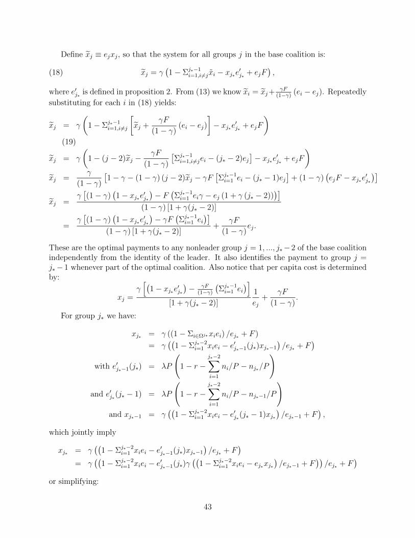
Define xj ≡ ejxj, so that the system for all groups j in the base coalition is:

(18) xj = γ(1− Σj∗−1

i=1,i 6=jxi − xj∗e′j∗ + ejF

),

where e′j∗ is defined in proposition 2. From (13) we know xi = xj+γF

(1−γ)(ei − ej). Repeatedly

substituting for each i in (18) yields:

xj = γ

(1− Σj∗−1

i=1,i 6=j

[xj +

γF

(1− γ)(ei − ej)

]− xj∗e′j∗ + ejF

)(19)

xj = γ

(1− (j − 2)xj −

γF

(1− γ)

[Σj∗−1i=1,i 6=jei − (j∗ − 2)ej

]− xj∗e′j∗ + ejF

)xj =

γ

(1− γ)

[1− γ − (1− γ) (j − 2)xj − γF

[Σj∗−1i=1 ei − (j∗ − 1)ej

]+ (1− γ)

(ejF − xj∗e′j∗

)]xj =

γ[(1− γ)

(1− xj∗e′j∗

)− F

(Σj∗−1i=1 eiγ − ej (1 + γ (j∗ − 2))

)](1− γ) [1 + γ(j∗ − 2)]

=γ[(1− γ)

(1− xj∗e′j∗

)− γF

(Σj∗−1i=1 ei

)](1− γ) [1 + γ(j∗ − 2)]

+γF

(1− γ)ej.

These are the optimal payments to any nonleader group j = 1, ..., j∗−2 of the base coalitionindependently from the identity of the leader. It also identifies the payment to group j =j∗− 1 whenever part of the optimal coalition. Also notice that per capita cost is determinedby:

xj =γ[(

1− xj∗e′j∗)− γF

(1−γ)

(Σj∗−1i=1 ei

)][1 + γ(j∗ − 2)]

1

ej+

γF

(1− γ).

For group j∗ we have:

xj∗ = γ ((1− Σi∈Ωj∗xiei) /ej∗ + F )

= γ((

1− Σj∗−2i=1 xiei − e′j∗−1(j∗)xj∗−1

)/ej∗ + F

)with e′j∗−1(j∗) = λP

(1− r −

j∗−2∑i=1

ni/P − nj∗/P

)

and e′j∗(j∗ − 1) = λP

(1− r −

j∗−2∑i=1

ni/P − nj∗−1/P

)and xj∗−1 = γ

((1− Σj∗−2

i=1 xiei − e′j∗(j∗ − 1)xj∗)/ej∗−1 + F

),

which jointly imply

xj∗ = γ((

1− Σj∗−2i=1 xiei − e′j∗−1(j∗)xj∗−1

)/ej∗ + F

)= γ

((1− Σj∗−2

i=1 xiei − e′j∗−1(j∗)γ((

1− Σj∗−2i=1 xiei − ej∗xj∗

)/ej∗−1 + F

))/ej∗ + F

)or simplifying:

43

xj∗ =γ

1− γ2e′j∗ (j∗−1)e′j∗−1(j∗)

ej∗ej∗−1

(1− Σj∗−2

i=1 xieiej∗

(1− γe′j∗−1(j∗)/ej∗−1

)+ F

(1− γe′j∗−1(j∗)/ej∗

)).

We can compute Σj∗−2i=1 xiei from (19) and it is a linear function of xj∗ :

Σj∗−2i=1 xiei =

γ[1− xj∗e′j∗(j∗ − 1)− γF

1−γΣj−1i=1ei

]Σj∗−2i=1 ei

1 + γ(j∗ − 2)+γF (j∗ − 2)

1− γ.

This implies:

xj∗ =

1−γ(1− γe′j∗−1(j∗)/ej∗−1

)γ

1+γ(j∗−2)

e′j∗ (j∗−1)

ej∗Σj∗−2i=1 ei

1− γ2e′j∗ (j∗−1)e′j∗−1(j∗)

ej∗ej∗−1

−1

∗ γ

1− γ2e′j∗ (j∗−1)e′j∗−1(j∗)

ej∗ej∗−1

∗

1− γ[1− γF1−γΣj−1

i=1 ei]Σj∗−2i=1 ei

1+γ(j∗−2)− γF (j∗−2)

1−γ

ej∗

(1− γe′j∗−1(j∗)/ej∗−1

)+ F

(1− γe′j∗−1(j∗)/ej∗

) .

For existence of an equilibrium without coups or revolutions it is necessary that for aleader randomly drawn from any group the value of patronage is large enough to ensure thatafter incentive compatible payments are made to elites required to ensure no revolutions,there still remains sufficient residual patronage for elites from the leader’s own ethnic groupto dissuade them mounting coups. A sufficient condition is that:

x1 =γ[(

1− xj∗e′j∗)− γF

(1−γ)

(Σj∗−1i=1 ei

)][1 + γ(j∗ − 2)]

1

e1

+γF

(1− γ)> 0.

This condition is sufficient, because if this holds for group 1 then it necessarily holds for allother groups as well since x1 < xi for all i > 1.

To prove uniqueness, we know that our equilibrium set of optimal transfers must satisfyx: xjej = γ (1− Σi∈Ωjxiei − x′(j)e′(j) + ejF ). Consider an alternative equilibrium denotedby ′′ for which x

′′j > xj. It follows from the equality two sentences previous that there must

exist at least one coalition member, k ∈ Ωj for which x′′

k < xk in this alternative equilibrium.But this immediately violates equation (14) above.

Since the solution to the set of equations (9) is unique, and these equations determinethe payments in equilibria consisting of a base set of ethnicities chosen by any leader, theoptimal coalitions defined in Proposition (2) will also apply whenever there exists a base setof ethnicities included in all governing coalitions. An alternative equilibrium set of paymentsand optimal coalition can only arise were there to be equilibria where there does not exist a‘base’ set of ethnicities chosen by all leaders. We have already shown in Lemma 1 that thiscannot occur.

44

No revolutions along the equilibrium path conditionIf (3)or (4) fails, then the indicator variable, <(Ω) = 1 always so that the government

faces a constant revolution. We thus have:

Wl(Ω) = ψΣi/∈ΩlniP

∗+V leaderl (Ω) ∗

(1− Σi/∈Ωlni

P

).

Note that we do not have to consider a leader constructing a coalition that included aninsider mounting revolutions against the government each period. If such a group wouldrevolt as insiders, they would also, at worse, revolt as outsiders, and they do not cost theleader patronage in that case, so they would not be included. A sufficient condition to ruleout constant revolutions is that it is not worthwhile for the leader to tolerate such revolutionsfrom even the smallest group of outsiders, nN . This group represents the lowest chance ofrevolution success, so a leader unwilling to bear this risk, will not bear it from any largerexcluded group. Let Ω

′denote the coalition formed by including all groups i 6= N. Thus we

have as a sufficient condition for no revolutions along the equilibrium path:

ψnNP∗+V leader

l (Ω′) ∗(

1− nnP

)< V leader

l (Ω) ,

This is satisfied for sufficiently low ψ, and we assume that ψ is sufficiently low so that thiscondition never binds.

No coups along the equilibrium path condition.We will now derive and discuss a sufficient condition for the leader’s choice of completely

ensuring against coups from any group j ∈ Ωl.Under xj solving (8) it is never worthwhile for an elite included in the coalition to

exercise his coup option. We now show the condition under which the leader will choose togive transfers solving (8). What is the alternative to solving this condition? It may be betterfor a leader to include a group so that it will not be willing to walk out and join a revolutionagainst the leader, but that it would still exercise a coup option if one arose. Under thiscondition, the xj given to it can be lower, denote it x′j. This x′j has to be high enough thatthe group j does not simply walk straight out and start a revolution, but not high enough sothat j will be loyal if he has a coup chance. This is solved as follows. Let V ′j

(Ωl)

denote thevalue to a member of group j in leader l′s coalition if he is receiving x′j < xj. The amountthat is just sufficient to stop a member of j forming a coalition against him is given by:(∑

i/∈Ωl ni + nj

P

)rV transition

j +

(1−

∑i/∈Ωl ni + nj

P

)rV 0

j = V ′j(Ωl)

.

Since V ′j(Ωl)

=x′j+δεV

transition

1−δ(1−ε) , V 0j = 0+δεV transition

1−δ(1−ε) and this implies

x′j = V transitionj

[(1− δ (1− ε))

(∑i/∈Ωl ni + nj

P

)r +

(1−

∑i/∈Ωl ni + nj

P

)rδε− δε

]The trade off faced by the leader is between personally saving

(xj − x′j

) ejel

and facing apossible coup if the opportunity arises for any member of group j. Notice that the trade off

45

is in theory ambiguous with respect to which size group should be paid below xj. A largegroup allows large savings, but it is also a very likely source of coups.

Similarly to the case of revolutions, we assume there is a personal cost ω > 0 associatedwith the leader falling victim of a coup (independently of winning or losing, as for revolu-tions). A sufficiently high loss ω will rule out any willingness by the leader of taking chanceswith coups. The condition for the leader to exclude coups from group j is:

xl + δ((1− ε)V leader

l

(Ωl)

+ εV transitionl

)≥(

1− γ ej∑i∈Ωl ei

)(xl +

ejel

(xj − x′j

)+ F + δ

((1− ε)V leader

l

(Ωl)

+ εV transitionl

))+γ

ej∑i∈Ωl ei

(−ω + δ

((1− ε)V loss

l + εV transitionl

)).

Notice that this condition is monotonic in the loss ω, hence there is always a sufficiently highcost of a coup so that the leader chooses to fully insure against it.

The rationale behind this sufficient condition is parsimony in the number of model pa-rameters to be estimated from the data. The advantage of this treatment is that since costω is not incurred on the equilibrium path, and we assume it is large enough so that theleader’s no coup condition never binds, ω will not enter into the estimating equations.

A final comment is in order. If a leader is victim of a coup, then he suffers a large oneperiod cost ω > 0. This is asymmetric in that such cost is not also incurred by the failedcoup leader, who only gets 0 upon failure in (8). We think of ω as the counterpart of theleadership premium F that the leader also receives asymmetrically. Leaders are differentfrom other elites: when you become a leader you obtain personal rents, but you also face arisk of a large negative cost if you are deposed.

Explicit form of V transitionj . Recall that this value function depends on the probability

of an elite in j being selected into a governing coalition by a new leader which we can, usingProposition 2, define.

V transitionj varies depending on whether an ethnicity is in the base group of larger eth-

nicities (and thus always included in leader’s optimal coalitions), or a smaller group (whoseinclusion in government only arises when one of their own is the leader), or one of the groupsj∗ and j∗ − 1 (whose inclusion in government depends on the size of the particular leader’sethnicity at the time). Specifically, from Proposition 2 it follows that:For j < j∗ − 1 :

V transitionj = pj (N) Vj

(Ωj)

+ (1− pj (N))Vj(Ωl).

For j = j∗ − 1 :

V transitionj∗−1 = pj∗−1 (N) Vj∗−1

(Ωj∗−1

)+

N∑l=1,l 6=[j∗,j+]

pl (N)Vj∗−1

(Ωl)

+

j+∑l=j∗

pl (N)

(e′j∗−1 (l)

ej∗−1

Vj∗−1

(Ωl)

+

(1−

e′j∗−1 (l)

ej∗−1

)V 0j∗−1

).

46

For j = j∗ :

V transitionj∗ = pj∗ (N) Vj∗

(Ωj∗)

+

j∗−1∑l=1

pl (N)

(e′j∗

ej∗Vj∗(Ωl)

+

(1−

e′j∗

ej∗

)V 0j∗

)+

N∑l=j+

pl (N)

(e′j∗ (l)

ej∗Vj∗(Ωl)

+

(1−

e′j∗ (l)

ej∗

)V 0j∗

)+

j+−1∑l=j∗+1

pl (N)V 0j∗ .

For j > j∗ :V transitionj = pj (N) Vj

(Ωj)

+ (1− pj (N))V 0j .

9.2 Theory Extensions: Elite – Non-Elite Divisions

A final issue worth addressing concerns the clientelistic microfoundations of the within-ethnic group organization34. In this section we answer the following questions: Why donon-elites support a leader who allocates a patronage position to their representative elite?How much of the value generated by such a patronage position does an elite keep, and howmuch does he have to share with his non-elite? Why do elites have incentives to organizetheir non-elites in support of a leader?

We define the patronage value of a government post (i.e., the dollar amount that aminister gets from controlling appointments, apportionment, acquisitions in his ministry) asV . V was normalized to 1 in Section 2, but we will keep it unnormalized here to focus onits explicit division between elite and non-elite. An elite member controlling x governmentposts controls a flow of resources xV . We still assume x is continuous and abstract from thediscreteness of post allocations.

Assume the use value of a government post to a member of the non-elite is U in totalif it is controlled by their own elite. If my group controls a ministry, I benefit by beingmore likely to be able to get benefits from this ministry. If it is education, for instance, mychildren will be more likely to access good schools. If it is public works, our people will bemore likely to get jobs in the sector and the benefits of good infrastructure. If it is the army,our men will be more likely to get commands. An empirical illustration of this logic for roadbuilding in Kenya is given by Burgess et al. (2010).

The use value of a post to the non-elite if it is controlled by someone else is φU . Letφ ≤ 1 be related to the degree of ethnic harmony. If φ = 1 non-elites do not care about theidentity of the minister, they get as much out of the ministry no matter who controls it. Ifφ = 0, society is extremely ethnically polarized. A ministry controlled by someone else is ofno use to me.

34We follow the intuition in Jackson and Roseberg (1982, p.40): “The arrangements by which regimesof personal rule are able to secure a modicum of stability and predictability have come to be spoken ofas ”clientilism”.....The image of clientilism is one of extensive patron-client ties. The substance and theconditions of such ties can be conceived of as the intermingling of two factors: first, the resources of patronage(and the interests in such resources, which can be used to satisfy wants and needs) may be regarded as themotivation for the personal contracts and agreements of which patron-client ties consist; and second theloyalty which transcends mere interests and is the social ‘cement’ that permits such ties to endure in theface of resource fluctuations. Both of these factors are important as an explanation for some of the stableelements in African personal rule.”

47

9.3 Nash Bargaining

The elite obtains posts in return for delivering support. The non-elites give support inreturn for having the control of posts in the hands of their own ethnic elites. We assumethat these two parties bargain over the allocation of the patronage value of the posts thatthe elite receive from the leader, xV . We also assume that they can commit to agreementsex ante. That is, if the non-elites withdraw support, a post will revert to some other ethnicelite member, with the consequent loss of value (1− φ)xU for them. If the elite loses thepatronage value of the post, he loses xV . This implies a Nash bargain, with κ denoting theshare of V going to the elite, as follows:

maxκ

(κxV − 0

1

)((1− κ)xV + (1− φ)xU

1/λ

)and implying that κ = 1+(1−φ)U

2V. So that the value to an elite of controlling x posts is:

κV x =1 + (1− φ)U

2x.

This result has several important implications. First of all, the greater the degree of ethnictension in a country (i.e. the lower φ), the greater the share of the value going to the eliteof each group is. Clearly, ethnic group leaders have incentive to incite ethnic tensions inthis setting in a fashion similar to Padro-i-Miquel (2007). High levels of ethnic tensions canproduce substantial inequality between the elite and the non-elite of ethnic groups. Secondly,the larger the use value of a government post to a member of the non-elite, U , the greaterthe share of the value going to the elite of each group.

Finally, suppose that the cost to an elite of organizing his 1/λ non-elite in support ofthe leader are c ≥ 0. For an elite from ethnicity j receiving xj posts for participating in thegovernment to be willing to participate in the government we have the following individualrationality constraint:

κV xj =1 + (1− φ)U

2xj ≥ c.

This must be satisfied for all groups in government. Let xIR ≡ c/1+(1−φ)U2

. Since xj issmaller for larger groups, it implies that if there exists some groups for whom xj < xIR thenthese will be paid xIR. This does not upset the ordering determined in Section 2, but doesrequire a re-calculation of the equilibrium patronage values. More interestingly, κ does affectthe share of post values accruing to the elite members, but does not affect the total numberof posts elites must receive from the leader, unless the participation constraint binds. Hence,particularly if φ affects ε adversely, country leaders will have strictly lower incentives to inciteethnic tension than ethnic group elites have. It is important to underscore the asymmetrybetween the incentives of leaders and ethnic group elites along this dimension.

48

REFERENCES

[1] Acemoglu, Daron and James Robinson. 2001. “A Theory of Political Transitions”American Economic Review, 91(4): 938-963.

[2] Acemoglu, Daron and James Robinson. 2005. Economic Origins of Dictatorshipand Democracy. Columbia University Press, New York.

[3] Acemoglu, Daron Georgy Egorov and Constantin Sonin. 2008. “Coalition For-mation in Non-Democracies”, Review of Economic Studies, 75: 987-1009.

[4] Adachi, Takanori and Yasutora Watanabe. 2007. “Ministerial Weights and Gov-ernment Formation: Estimation Using a Barganing Model” Journal of Law, Economics,and Organization. 24(1).

[5] Aghion, Phillipe, Alberto Alesina, and Francesco Trebbi. 2004. “EndogenousPolitical Institutions.” Quarterly Journal of Economics. 119(2), May.

[6] Alesina, Alberto, Arnaud Devleeshauwer, William Easterly, Sergio Kurlat,Romain Wacziarg. 2003.“Fractionalization” Journal of Economic Growth, 8(2): 155-194

[7] Ansolabehere, Stephen, Snyder, James, Aaron B. Strauss, and Michael M.Ting. 2005. “Voting Weights and Formateur Advantages in the Formation of CoalitionGovernments” American Journal of Political Science, 49(3): 550-563.

[8] Arriola, Leonardo R. 2009. “Patronage and Political Stability in Africa” ComparativePolitical Studies, 42(10), 1339-62.

[9] Baron, David and John Ferejohn (1989), “Bargaining in Legislatures” AmericanPolitical Science Review 83 (December), 1181

[10] Baumol, William J., John C. Panzar and Robert D. Willig. 1982. ContestableMarkets and the Theory of Industry Structure. New York: Harcourt Brace Jovanovich.

[11] Bates, Robert. 1981. Markets and States in Tropical Africa: The Poltical Basis ofAgricultural Policies. University of California Press.

[12] Berman, Bruce. 1998. “Ethnicity, Patronage and the African State: The Politics ofUncivil Nationalism.” African Affairs 97:305-341.

[13] Besley, Timothy and Torsten Persson. 2011. Pillars of Prosperity: The PoliticalEconomics of Development Clusters, Princeton, NJ: Princeton University Press.

[14] Bienen, John, Henry Londregan and Nicolas van de Walle. 1995. “Ethnicityand Leadership Succession in Africa.” International Studies Quarterly, 39(1):1-25.

[15] Breusch, T.S. and Adrian R. Pagan. 1980. “The Lagrange Multiplier Test and ItsApplications to Model Specifications in Econometrics”, Review of Economic Studies,47: 239-253.

49

[16] Bueno de Mesquita, Bruce, Alastair Smith, Randolph Siverson, and JamesD. Morrow. 2003. The Logic of Political Survival. MIT Press, Cambridge.

[17] Burgess, Robin, Remi Jedwaby, Edward Miguel, Ameet Morjaria, and Ger-ard Padro i Miquel. 2011. “Ethnic Favoritism” mimeo LSE.

[18] Carey, J., and Hix, S. 2011. “The electoral sweet spot: Low-magnitude proportionalelectoral systems”. American Journal of Political Science, 55, 383-397.

[19] Clarke, Kevin A. 2003. “Nonparametric Model Discrimination in International Rela-tions,” Journal of Conflict Resolution, 47(1), 72-93.

[20] Diermeier, Daniel, Hulya Eraslan, and Antonio Merlo. 2003. “A StructuralModel of Government Formation” Econometrica, 71(1): 27-70.

[21] Diermeier, Daniel and Antonio Merlo. 2004. “An Empirical Investigation of Coali-tional Barganing Procedures” Journal of Public Economics, 88(3-4): 783-797.

[22] Diermeier, Daniel and Randy Stevenson. 1999. “Cabinet Survival and CompetingRisks” American Journal of Political Science, 43(5): 1051-1098.

[23] Easterly, William R. and Levine, Ross. 1997. “Africa’s Growth Tragedy: Policiesand Ethnic Divisions.” Quarterly Journal of Economics, November 1997, 112(4), pp.1203-50.

[24] Fearon, James D. 2003. “Ethnic and Cultural Diversity by Country” Journal of Eco-nomic Growth, 8(2): 195-222.

[25] Fearon, James D. and David D. Laitin. 2003. “Ethnicity, Insurgency, and CivilWar” American Political Science Review, 97(1): 75-90.

[26] Francois, Patrick, Ilia Rainer, and Francesco Trebbi. 2012. “The Dictator’s InnerCircle.” mimeo UBC.

[27] Gandhi, Jennifer and Przeworski, Adam. 2006. “Cooperation, cooptation andrebellion under dictatorship.” Economics and Politics, 18(1), 1-26.

[28] Gallagher, Michael. 1991. “Proportionality, Disproportionality, and Electoral Sys-tems”. Electoral Sudies 10:33-51.

[29] Geddes, Barbara. 2003. Paradigms and sand castles: Research design in comparativepolitics. Ann Arbor: University of Michigan Press.

[30] Jackson RH and CG Rosberg. 1982. Personal Rule in Black Africa: Prince, Auto-crat, Prophet, Tyrant. UC Berkely Press CA.

[31] Khapoya, Vincent. 1980. “Kenya Under Moi: Continuity or Change?” Africa Today,27(1), 17-32.

50

[32] Kotze Hennie and Caryl Steyn. 2003. African Elite Perspectives: AU and NEPAD.A Comparative Study Across Seven African Countries Konrad-Adenauer-Stiftung: Jo-hannesburg, South Africa.

[33] Kramon, Erik and Daniel Posner. 2011. “Ethnic Favoritism in Primary Educationin Kenya” mimeo MIT.

[34] Merlo, Antonio. 1997. “Bargaining Over Governments in a Stochastic Environment”Journal of Political Economy, 105: 101-131.

[35] Michalopoulos, Stelios. 2012. “The Origins of Ethnolinguistic Diversity” AmericanEconomic Review, 102(4): 1508-39.

[36] Michalopoulos, Stelios and Elias Papaioannou. 2011. “The Long-Run Effects ofthe Scramble For Africa” NBER WP 17620.

[37] Mulligan, C. and K. Tsui. 2008. “Causes and Consequences of Political Competi-tiveness” mimeo University of Chicago.

[38] Osaghae, Eghosa E. 1989. “The Federal Cabinet, 1951-1984.” In Federal Characterand Federalism in Nigeria, edited by Peter Ekeh and Eghosa Osaghae. Ibadan: Heine-mann Educational Books.

[39] Padro-i-Miquel, Gerard. 2007. “The Control of Politicians in Divided Societies: ThePolitics of Fear”, Review of Economic Studies, 74(4): 1259-127.

[40] Posner, Daniel 2004. “Measuring Ethnic Fractionalization in Africa.” American Jour-nal of Political Science, 48: 849–863.

[41] Posner, Daniel. 2005. Institutions and Ethnic Politics in Africa. Cambridge: Cam-bridge University Press.

[42] Posner, Daniel and Daniel Young. 2007. “The Institutionalization of Political Powerin Africa.” Journal of Democracy 18(3).

[43] Rainer, Ilia and Francesco Trebbi. 2011. “New Tools for the Analysis of PoliticalPower in Africa.” NBER Africa Project Volume.

[44] Roessler, Philip. 2011. “The Enemy Within: Personal Rule, Coups and Civil War inAfrica” World Politics 63(2): 300-346.

[45] Tullock,Gordon. 1987. Autocracy. Kluwer Academic Publishers, The Netherlands.

[46] Vuong, Quang H. 1989. “Likelihood Ratio Tests for Model Selection and Non-NestedHypotheses,” Econometrica, 2, 307-333

[47] Wintrobe, Ronald. 1998. The Political Economy of Dictatorship. Cambridge: Cam-bridge University Press.

[48] Wittman, Donald A.1995. The Myth of Democratic Failure: Why Political Institu-tions are Efficient. Chicago: University of Chicago Press.

51

Table 1: African Cabinets - Summary Statistics by Country

Number of Percent of

Average Total Average Government- Government-

Time Years Number of Number of Size of Number of Number of Number

of Ministers Ministers

Period Years with Two Number of Leaders Government- Government Unique Governments Ethnic with Missing with Missing

Country Covered Missing Governments Governments in Power Ministers (# posts) Ministers per Minister Groups Ethnicity Ethnicity

Benin 1960-2004 1969, 1975 1968, 1970 45 10 730 16.22 209 3.49 15 1 0.14%

Cameroon 1960-2004 1969, 1975 1968 44 2 1445 32.84 262 5.52 21 43 2.98%

Cote d'Ivoire 1960-2004 1975 1970 45 4 1256 27.91 233 5.39 17 0 0%

Dem. Rep. Congo 1961-2004 1972, 1974 1970, 1973 44 4 1352 30.73 515 2.63 30 5 0.37%

Gabon 1960-2004 1975 44 2 1173 26.66 185 6.34 10 6 0.51%

Ghana 1960-2004 1975 1970 45 9 1140 25.33 362 3.15 22 0 0%

Guinea 1960-2004 1975 1969 45 2 1213 26.96 244 4.97 9 4 0.33%

Kenya 1964-2004 1975 1970 41 3 1010 24.63 155 6.52 16 2 0.20%

Liberia 1960-2004 1975 1970 45 10 938 20.84 272 3.45 15 9 0.96%

Nigeria 1961-2004 1975 1970 44 11 1499 34.07 473 3.17 17 13 0.87%

Rep. of Congo 1960-2004 1969, 1975 1968, 1970 45 7 918 20.40 239 3.84 10 9 0.98%

Sierra Leone 1960-2004 1972, 1975 1970, 1973 45 9 1109 24.64 288 3.85 14 0 0%

Tanzania 1965-2004 1972, 1974 1970, 1973 40 3 1016 25.40 158 6.43 37 0 0%

Togo 1960-2004 1975 1970 45 3 757 16.82 199 3.80 20 0 0%

Uganda 1963-2004 1972, 1974 1970, 1973 42 6 1037 24.69 205 5.06 26 3 0.29%

Notes: In the "Number of Leaders in Power" column, we count a new nonconsecutive term in office of the same leader as a new leader. Source: Rainer and Trebbi (2011).

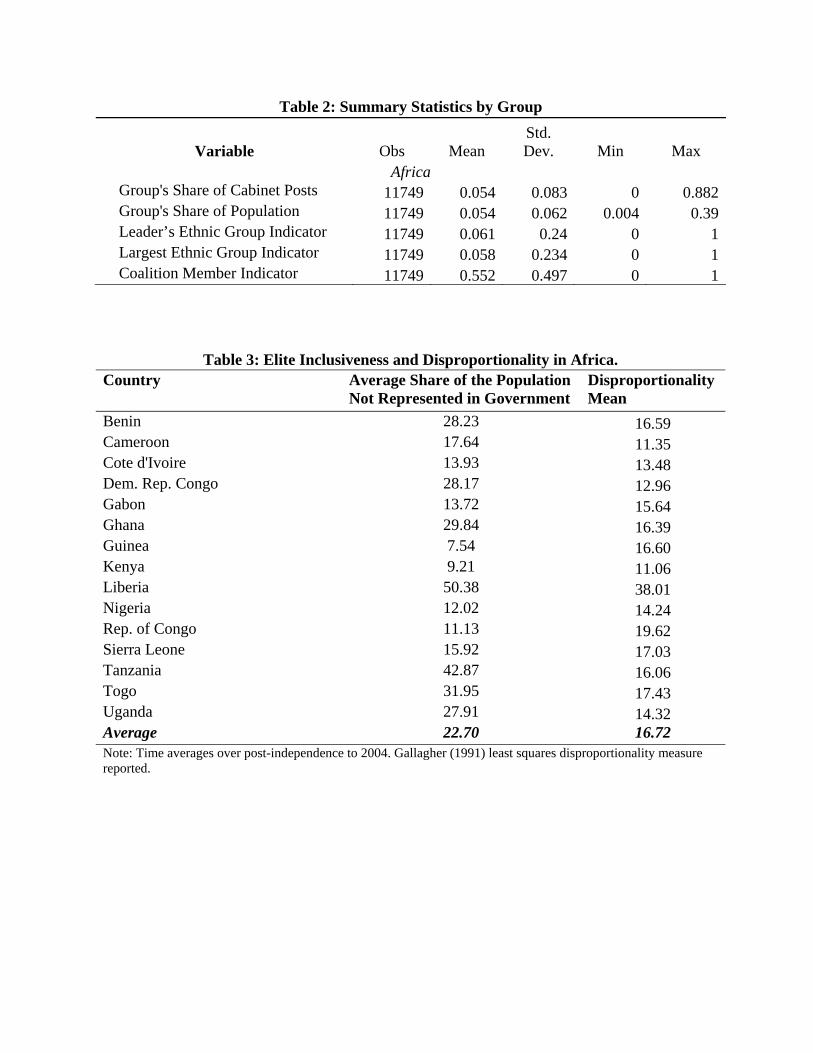
Table 2: Summary Statistics by Group

Variable Obs Mean Std. Dev. Min Max

Africa Group's Share of Cabinet Posts 11749 0.054 0.083 0 0.882Group's Share of Population 11749 0.054 0.062 0.004 0.39Leader’s Ethnic Group Indicator 11749 0.061 0.24 0 1Largest Ethnic Group Indicator 11749 0.058 0.234 0 1Coalition Member Indicator 11749 0.552 0.497 0 1

Table 3: Elite Inclusiveness and Disproportionality in Africa. Country Average Share of the Population

Not Represented in Government Disproportionality Mean

Benin 28.23 16.59 Cameroon 17.64 11.35 Cote d'Ivoire 13.93 13.48 Dem. Rep. Congo 28.17 12.96 Gabon 13.72 15.64 Ghana 29.84 16.39 Guinea 7.54 16.60 Kenya 9.21 11.06 Liberia 50.38 38.01 Nigeria 12.02 14.24 Rep. of Congo 11.13 19.62 Sierra Leone 15.92 17.03 Tanzania 42.87 16.06 Togo 31.95 17.43 Uganda 27.91 14.32 Average 22.70 16.72 Note: Time averages over post-independence to 2004. Gallagher (1991) least squares disproportionality measure reported.

Table 4: Group Size, Leadership, and Cabinet Membership, 1960-2004. All Ethnic Groups

Is in Government Coalition?

Is in Government Coalition?

Is Leader Group?

Is Leader Group?

(1) (2) (3) (4) Group Size 6.5887 8.0741 0.5353 0.5807

(1.0925) (0.6245) (0.0871) (0.1540) Largest Group -0.5702 -0.0125

(0.0593) (0.0356) Country FE Yes Yes Yes Yes

Year FE Yes Yes Yes Yes N 11,749 11,749 11,749 11,749

Notes: Dep. Var. (1), (2) = Dummy for membership of the ruling coalition. Dep. Var. Cols. (3), (4) = Dummy for the group being the ethnicity of the leader. Group Size = Ethnic Share of Population. Largest Group = Largest Ethnic Group. Probit marginal effects and standard errors clustered at the country level in parentheses below.

Table 5: Leadership in Cabinet Formation, Group Size, and Allocation of Cabinet Seats, 1960-2004. All Ethnic Groups

Share of All Cabinet

Seats

Share of All Cabinet

Seats

Share of All Cabinet

Seats

Share of Top

Cabinet Seats

Share of Top

Cabinet Seats

Share of Top

Cabinet Seats

(1) (2) (3) (4) (5) (6) Group Size 0.7740 1.0118 1.0198 0.7649 0.9033 0.8869

(0.0755) (0.1482) (0.1228) (0.0713) (0.1667) (0.1398) Group Size2 -0.924 -0.945 -0.538 -0.560

(0.445) (0.405) (0.613) (0.517) Leader Group 0.1126 0.1108 0.2084 0.2073

(0.0270) (0.0271) (0.0257) (0.0258) Country FE Yes Yes Yes Yes Yes Yes

Year FE Yes Yes Yes Yes Yes Yes R2 0.55 0.55 0.50 0.49 0.49 0.30 N 11,749 11,749 11,029 11,749 11,749 11,029

Notes: Dep. Var. Cols. (1)-(3) = Share of All Cabinet Posts Reported. Dep. Var. (4)-(6) = Share of Top Cabinet Posts (Presidency/Premiership, Defense, Budget, Commerce, Finance, Treasury, Economy, Agriculture, Justice, Foreign). Columns (3) and (6) exclude the leader’s ethnic group in each country-year. Standard errors clustered at the country level in parentheses below coefficients. Group Size = Ethnic Share of Population. Group size squared coefficient and standard errors are x10,000.

Table 6: Full Cabinet - Maximum Likelihood Estimates 11.5 (1.4) 0.115 (0.012) 0.95

Country r F logLL Insider IC constraint

violated? Benin 63.5 0.893 1.0e-13 1.2e+13 106.8494 no (5.0) (0.011) (0.018) (2.1e24)Cameroon 254.5 0.9692 3.8e-13 2.6e+12 589.6414 no (15.3) (0.0047) (0.0083) (5.5e+23)Congo, D. Rep. 178.8 0.886 0.200 3.99 514.6169 no (10.3) (0.011) (0.034) (0.95)Cote d'Ivoire 172.7 0.9209 0.381 0.33 418.7874 no (11.8) (0.0076) (0.016) (0.12)Gabon 72.9 0.9847 3.8e-11 2.5e+10 201.4787 no (6.8) (0.0092) (0.081) (5.3e+19)Ghana 79.6 0.854 0.77 0.41 150.2744 no (4.8) (0.013) (0.38) (0.89)Guinea 126.7 0.9909 0.089 6.9 270.5889 no (10.5) (0.0035) (0.021) (2.1)Kenya 250.9 0.9667 0.107 6.9 562.5347 no (14.5) (0.0042) (0.025) (2.0)Liberia 24.5 0.894 0.233 -2.26 -67.6506 yes (2.0) (0.014) (0.056) (0.23)Nigeria 139.9 0.9577 0.385 1.03 521.5482 no (7.3) (0.0046) (0.045) (0.22)Rep. of Congo 76.0 0.9317 0.498 0.000 261.4404 no (5.2) (0.0071) (0.033) (0.086)Sierra Leone 69.8 0.9010 0.574 0.262 180.2609 no (5.2) 0.0092) (0.034) (0.051)Tanzania 142.8 1.0000 0.112 4.84 337.3617 no (7.2) (0.0058) (0.040) (2.56)Togo 53.6 0.840 0.582 0.34 45.4974 no (4.2) (0.014) (0.060) (0.17)Uganda 134.3 0.929 1.0000 1.5e-12 273.8432 no (8.5) (0.016) (8.1e-8) (1.4e-7) Notes: Asymptotic Standard Errors in Parentheses. The logLL reported is specific to the contribution of each country. The insider constraint of a unilateral deviation of a coalition member is checked ex post in the last column. This is constraint (4) in the text.

Table 7: Full Cabinet - Slopes and Leadership Premia

Country Slope:

FLeadership

Premium Benin 1.26 0.120 (0.034) (0.025)Cameroon 0.98 0.086 (0.016) (0.008)Congo, D. Rep. 1.00 0.074 (0.040) (0.009)Cote d'Ivoire 0.20 0.148 (0.066) (0.008)Gabon 0.93 0.100 (0.058) (0.020)Ghana 1.36 0.016 (0.120) (0.021)Guinea 0.67 0.199 (0.032) (0.010)Kenya 0.82 0.105 (0.029) (0.006)Liberia -0.69 0.430 (0.260) (0.041)Nigeria 0.64 0.058 (0.035) (0.008)Rep. of Congo 0.00 0.270 (0.085) (0.009)Sierra Leone 0.35 0.198 (0.055) (0.016)Tanzania 0.60 0.070 (0.095) (0.015)Togo 0.48 0.234 (0.140) (0.013)Uganda 1.68 -2.7e-14 (0.053) (2.1e-9)Average (excluding LIB) 0.78 0.12Notes: Asymptotic Standard Errors in Parentheses.

Table 8: Top Cabinet Posts Only - Maximum Likelihood Estimates 11.5 (1.4) 0.115 (0.012) 0.95

Country r F logLL Insider IC constraint

violated? Benin 18.6 0.821 0.35 2.0 209.9855 no (2.1) (0.016) (0.18) (2.1)Cameroon 40.1 0.837 0.443 0.27 259.4370 no (3.9) (0.014) (0.067) (0.41)Congo, D. Rep. 29.3 0.853 0.053 20.4 485.2384 no (2.9) (0.014) (0.056) (25.5)Cote d'Ivoire 22.9 0.910 0.116 1.59 281.0537 no (2.9) (0.015) (0.041) (2.21)Gabon 18.9 0.815 5.6e-13 2.5e+12 57.2651 no (2.1) (0.017) (0.33) (1.6e+24)Ghana 10.4 0.816 0.29 1.36 488.0237 no (1.0) (0.016) (0.18) (2.91)Guinea 25.9 0.919 0.405 0.43 19.3376 no (2.9) (0.008) (0.079) (0.32)Kenya 23.4 0.907 6.2e-15 6.0e+14 152.3001 no (2.5) (0.016) (0.004) (1.1e+26)Liberia 10.8 1.000 0.071 -3.0121 282.3815 yes (1.6) (0.023) (0.029) (1.3e-5)Nigeria 27.6 0.9218 0.275 1.47 180.0479 no (2.7) (0.0085) (0.071) (0.83)Rep. of Congo 19.7 0.9057 0.583 -0.48 75.7406 no (2.2) (0.0093) (0.058) (0.10)Sierra Leone 16.6 0.897 0.36 1.35 205.9451 no (1.3) 0.012) (0.10) (0.79)Tanzania 43.0 0.876 0.249 0.18 403.8598 no (4.0) (0.012) (0.042) (0.55)Togo 15.8 0.836 0.411 0.36 382.4744 no (2.1) (0.014) (0.082) (0.45)Uganda 24.5 0.832 9.8e-14 1.5e+13 439.4047 no (2.5) (0.015) (0.03) (4.7e+24) Notes: Asymptotic Standard Errors in Parentheses. The logLL reported is specific to the contribution of each country. The insider constraint of a unilateral deviation of a coalition member is checked ex post in the last column. This is constraint (4) in the text.

Table 9: Top Cabinet Posts Only - Slopes and Leadership Premia

Country Slope:

FLeadership

Premium Benin 1.06 0.282 (0.31) (0.030)Cameroon 0.22 0.312 (0.27) (0.018)Congo, D. Rep. 1.13 0.207 (0.15) (0.028)Cote d'Ivoire 0.21 0.436 (0.21) (0.031)Gabon 1.44 0.347 (0.34) (0.026)Ghana 0.57 0.346 (0.74) (0.044)Guinea 0.30 0.293 (0.13) (0.026)Kenya 0.989 0.282 (0.058) (0.023)Liberia -0.23 0.572 (0.10) (0.074)Nigeria 0.56 0.209 (0.13) (0.033)Rep. of Congo -0.67 0.319 (0.22) (0.028)Sierra Leone 0.68 0.223 (0.14) (0.037)Tanzania 0.06 0.152 (0.17) (0.020)Togo 0.25 0.341 (0.25) (0.030)Uganda 1.483 0.243 (0.086) (0.026)Average (excluding LIB) 0.59 0.28Notes: Asymptotic Standard Errors in Parentheses.

Table 10: Specification Tests

Full Sample. Generalized likelihood ratio tests: Null is equivalent fit between the specified model and the Baseline model

Model Log-likelihood

Vuong test statistic

p-value

Clarke test statistic

p-value

Baseline 4367.1 - - - -Random Allocation 3136.7 19.0 0.000 7478 0.000Big Man Allocation -5134.2 60.1 0.000 6070 0.000Observations 11749Note: Clarke statistic corresponds to number of positive differences between log likelihoods. The null corresponds to Observations/2=5875 positive differences. Vuong test statistic is distributed N(0,1).

Military Regimes Only. Generalized likelihood ratio tests: Null is equivalent fit between the specified model and the Baseline model

Model Log-likelihood

Vuong test statistic

p-value

Clarke test statistic

p-value

Baseline 2099.2 - - - -Random Allocation 1400.1 13.7 0.000 3270 0.000Big Man Allocation -2282.1 40.1 0.000 2699 0.000Observations 5156Note: Clarke statistic corresponds to number of positive differences between log likelihoods. The null corresponds to Observations/2=2578 positive differences. Vuong test statistic is distributed N(0,1).

Civilian Regimes Only. Generalized likelihood ratio tests: Null is equivalent fit between the specified model and the Baseline model

Model Log-likelihood

Vuong test statistic

p-value

Clarke test statistic

p-value

Baseline 2552.7 - - - -Random Allocation 1880.1 12.4 0.000 3976 0.000Big Man Allocation -2832.2 44.5 0.000 3381 0.036Observations 6593Note: Clarke statistic corresponds to number of positive differences between log likelihoods. The null corresponds to Observations/2=3297 positive differences. Vuong test statistic is distributed N(0,1).

Table 10: Specification Tests (cont.)

Autocratic Regimes Only. Generalized likelihood ratio tests: Null is equivalent fit between the specified model and the Baseline model

Model Log-likelihood

Vuong test statistic

p-value

Clarke test statistic

p-value

Baseline 4173.6 - - - -Random Allocation 2986.3 18.8 0.000 6910 0.000Big Man Allocation -4799.0 58.2 0.000 5699 0.000Observations 11013Note: Clarke statistic corresponds to number of positive differences between log likelihoods. The null corresponds to Observations/2=5507 positive differences. Vuong test statistic is distributed N(0,1).

Democratic Regimes Only. Generalized likelihood ratio tests: Null is equivalent fit between the specified model and the Baseline model

Model Log-likelihood

Vuong test statistic

p-value

Clarke test statistic

p-value

Baseline Model 278.8 - - - -Random Allocation 183.1 -3.5 0.000 234 0.000Big Man Allocation -318.9 12.7 0.000 366 0.682Observations 722Note: Clarke statistic corresponds to number of positive differences between log likelihoods. The null corresponds to Observations/2=361 positive differences. Vuong test statistic is distributed N(0,1). Note: Values in bold indicate the test rejects equal fit of the models in favor of the main baseline model against the alternative model. Positive log-likelihood values are a natural occurrence in censored models.

Figure 1: Disproportionality in Cabinet Allocation, African Sample, 1960-2004

03

060

030

60

03

060

030

60

1960 1980 2000

1960 1980 2000 1960 1980 2000 1960 1980 2000

Benin Cameroon CongoKinshasa Cote d'Ivoire

Gabon Ghana Guinea Kenya

Liberia Nigeria Republic of Congo Sierra Leone

Tanzania Togo Uganda

LS

q D

ispr

opo

rtio

nal

ity

YearGraphs by Country

Figure 2: Allocation of Cabinet Shares and Population Shares. 1960-2004

0.1

.2.3

.4.5

Eth

nic

Gro

up'

s C

abin

et S

har

e

0 .1 .2 .3 .4 .5Ethnic Group's Population Share

Share of Posts to Non-leader Groups

Lowess Fit

Linear Fit

45 Degrees

Figure 3: Difference between Cabinet Shares and Population Shares. Guinea, 1960-2004

Figure 4: Difference between Cabinet Shares and Population Shares. Kenya, 1960-2004

-20

02

0-2

00

20

-20

02

0

1960 1980 2000

1960 1980 2000 1960 1980 2000

Fulani Kissi Kpelle

Malinke Mano Susu

Toma Yalunka

If Leader Group If Not Leader

Leader Transition

Share of Cabinet Seats - Pop. Share in Guinea

Graphs by Ethnicity

-20

020

-20

020

-20

020

-20

020

1960 1980 2000

1960 1980 2000 1960 1980 2000 1960 1980 2000

Boran Embu Kalenjin Kamba

Kikuyu Kisii Luhya Luo

Masai Meru Mijikenda Rendille

Somali Taita Turkana

If Leader Group If Not Leader

Leader Transition

Share of Cabinet Seats - Pop. Share in Kenya

Graphs by Ethnicity

Figure 5: In-Sample Fit of Coalition Size

Figure 6: In-Sample Successfully Predicted Groups in % of Population

0.000

0.100

0.200

0.300

0.400

0.500

0.600

0.700

0.800

0.900

1.000

Coalition size (fraction of population)

Predicted

Observed

Ben

in

Cam

eroo

n

Con

go

Cot

e d'

Ivoi

re

Gab

on

Gha

na Gui

nea

Ken

ya

Libe

ria

Nig

eria

Rep

. of C

ongo

Sie

rra

Leon

e

Tan

zani

a

Tog

o

Uga

nda

0.000

0.100

0.200

0.300

0.400

0.500

0.600

0.700

0.800

0.900

1.000

Correct predictions (fraction of population)

Predicted out

Predicted in

Figure 7: In-Sample Leadership Shares

Figure 8: In-Sample Shares to Largest Group

0.000

0.100

0.200

0.300

0.400

0.500

0.600

Leadership share

Predicted

Observed

0.000

0.050

0.100

0.150

0.200

0.250

0.300

0.350

0.400

Largest ethnicity share

Predicted

Observed

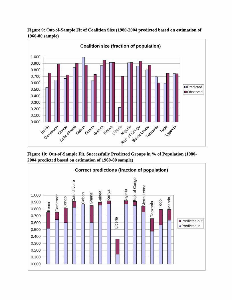
Figure 9: Out-of-Sample Fit of Coalition Size (1980-2004 predicted based on estimation of 1960-80 sample)

Figure 10: Out-of-Sample Fit, Successfully Predicted Groups in % of Population (1980-2004 predicted based on estimation of 1960-80 sample)

0.000

0.100

0.200

0.300

0.400

0.500

0.600

0.700

0.800

0.900

1.000

Coalition size (fraction of population)

PredictedObserved

Ben

in

Cam

eroo

n

Con

go Cot

e d'

Ivoi

re

Gab

on

Gha

na

Gui

nea

Ken

ya

Libe

ria

Nig

eria

Rep

. of C

ongo

Sie

rra

Leon

e

Tan

zani

a

Tog

o

Uga

nda

0.000

0.100

0.200

0.300

0.400

0.500

0.600

0.700

0.800

0.900

1.000

Correct predictions (fraction of population)

Predicted outPredicted in

Figure 11: Out-of-Sample Fit of Leadership Shares (1980-2004 predicted based on estimation of 1960-80 sample)

Figure 12: Out-of-Sample Fit, Shares to Largest Group (1980-2004 predicted based on estimation of 1960-80 sample)

0.000

0.100

0.200

0.300

0.400

0.500

0.600

0.700

0.800

0.900

1.000

Leadership share

PredictedObserved

0.000

0.050

0.100

0.150

0.200

0.250

0.300

0.350

0.400

0.450

Largest ethnicity share

Predicted

Observed

Figure 13: Counterfactual Coalition Size (1980-2004 predicted based on estimation of 1960-80 sample). r/r = -.1

Figure 14: Counterfactual Shares to Leader’s Group (1980-2004 predicted based on estimation of 1960-80 sample). r/r = -.1

0.0000.1000.2000.3000.4000.5000.6000.7000.8000.9001.000

Coalition size (fraction of population)

PredictedCounterfactual

0.000

0.200

0.400

0.600

0.800

1.000

1.200

Leadership share

Predicted

Counterfactual

Figure 15: Counterfactual Shares to Largest Group (1980-2004 predicted based on estimation of 1960-80 sample). r/r = -.1

Figure 16: Counterfactual Coalition Size (1980-2004 predicted based on estimation of 1960-80 sample). / = -.25

0.000

0.100

0.200

0.300

0.400

0.500

0.600

0.700

0.800

Largest ethnicity share

PredictedCounterfactual

0.0000.1000.2000.3000.4000.5000.6000.7000.8000.9001.000

Coalition size (fraction of population)

PredictedCounterfactual

Figure 17: Counterfactual Shares to Leader’s Group (1980-2004 predicted based on estimation of 1960-80 sample). / = -.25

Figure 18: Counterfactual Shares to Largest Group (1980-2004 predicted based on estimation of 1960-80 sample). /= -.25

0.000

0.100

0.200

0.300

0.400

0.500

0.600

0.700

0.800

0.900

1.000

Leadership share

Predicted

Counterfactual

0.000

0.050

0.100

0.150

0.200

0.250

0.300

0.350

0.400

0.450

Largest ethnicity share

PredictedCounterfactual

Figure 19: Counterfactual Coalition Size (1980-2004 predicted based on estimation of 1960-80 sample). F/F = -.25

Figure 20: Counterfactual Shares to Leader’s Group (1980-2004 predicted based on estimation of 1960-80 sample). F/F = -.25

0.0000.1000.2000.3000.4000.5000.6000.7000.8000.9001.000

Coalition size (fraction of population)

PredictedCounterfactual

0.000

0.100

0.200

0.300

0.400

0.500

0.600

0.700

0.800

0.900

1.000

Leadership share

Predicted

Counterfactual

Figure 21: Counterfactual Shares to Largest Group (1980-2004 predicted based on estimation of 1960-80 sample). F/F = -.25

Figure 22: Counterfactual Coalition Size (1980-04 predicted based on estimation of 1960-80 sample). Counterfactual distribution ni= ni - 1% for i=1,..,N/2-1; ni= ni + 1% for i=N/2+1,..,N.

0.000

0.050

0.100

0.150

0.200

0.250

0.300

0.350

0.400

0.450

Largest ethnicity share

PredictedCounterfactual

0.0000.1000.2000.3000.4000.5000.6000.7000.8000.9001.000

Coalition size (fraction of population)

PredictedCounterfactual

Figure 23: Counterfactual Shares to Leader’s Group (1980-04 predict. based on estimation of 1960-80 sample). Counterfactual ni= ni - 1% for i=1,..,N/2-1; ni= ni + 1% for i=N/2+1,..,N.

Figure 24: Counterfactual Shares to Largest Group (1980-04 predict. based on estimation of 1960-80 sample). Counterfactual ni= ni - 1% for i=1,..,N/2-1; ni= ni + 1% for i=N/2+1,..,N.

0.000

0.200

0.400

0.600

0.800

1.000

1.200

Leadership share

PredictedCounterfactual

0.000

0.050

0.100

0.150

0.200

0.250

0.300

0.350

0.400

0.450

Largest ethnicity share

Predicted

Counterfactual

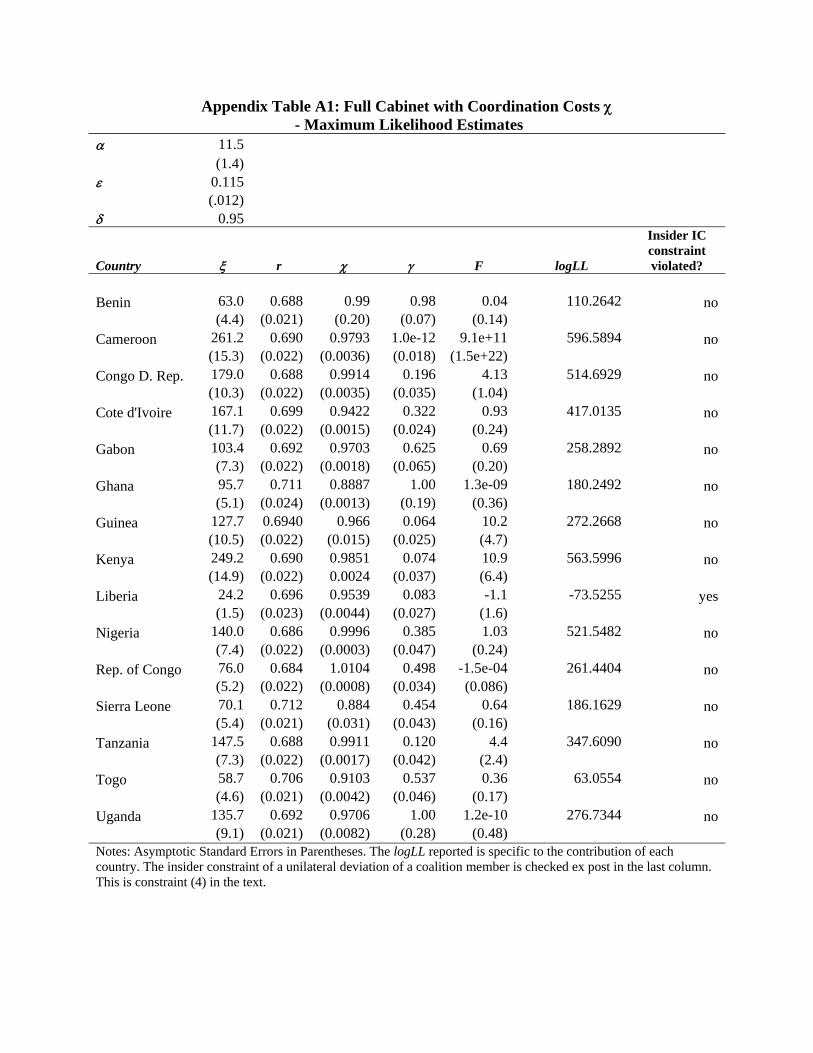
Appendix Table A1: Full Cabinet with Coordination Costs - Maximum Likelihood Estimates

11.5 (1.4) 0.115 (.012) 0.95

Country r F logLL

Insider IC constraint violated?

Benin 63.0 0.688 0.99 0.98 0.04 110.2642 no (4.4) (0.021) (0.20) (0.07) (0.14) Cameroon 261.2 0.690 0.9793 1.0e-12 9.1e+11 596.5894 no (15.3) (0.022) (0.0036) (0.018) (1.5e+22) Congo D. Rep. 179.0 0.688 0.9914 0.196 4.13 514.6929 no (10.3) (0.022) (0.0035) (0.035) (1.04) Cote d'Ivoire 167.1 0.699 0.9422 0.322 0.93 417.0135 no (11.7) (0.022) (0.0015) (0.024) (0.24) Gabon 103.4 0.692 0.9703 0.625 0.69 258.2892 no (7.3) (0.022) (0.0018) (0.065) (0.20) Ghana 95.7 0.711 0.8887 1.00 1.3e-09 180.2492 no (5.1) (0.024) (0.0013) (0.19) (0.36) Guinea 127.7 0.6940 0.966 0.064 10.2 272.2668 no (10.5) (0.022) (0.015) (0.025) (4.7) Kenya 249.2 0.690 0.9851 0.074 10.9 563.5996 no (14.9) (0.022) 0.0024 (0.037) (6.4) Liberia 24.2 0.696 0.9539 0.083 -1.1 -73.5255 yes (1.5) (0.023) (0.0044) (0.027) (1.6) Nigeria 140.0 0.686 0.9996 0.385 1.03 521.5482 no (7.4) (0.022) (0.0003) (0.047) (0.24) Rep. of Congo 76.0 0.684 1.0104 0.498 -1.5e-04 261.4404 no (5.2) (0.022) (0.0008) (0.034) (0.086) Sierra Leone 70.1 0.712 0.884 0.454 0.64 186.1629 no (5.4) (0.021) (0.031) (0.043) (0.16) Tanzania 147.5 0.688 0.9911 0.120 4.4 347.6090 no (7.3) (0.022) (0.0017) (0.042) (2.4) Togo 58.7 0.706 0.9103 0.537 0.36 63.0554 no (4.6) (0.021) (0.0042) (0.046) (0.17) Uganda 135.7 0.692 0.9706 1.00 1.2e-10 276.7344 no (9.1) (0.021) (0.0082) (0.28) (0.48) Notes: Asymptotic Standard Errors in Parentheses. The logLL reported is specific to the contribution of each country. The insider constraint of a unilateral deviation of a coalition member is checked ex post in the last column. This is constraint (4) in the text.