how important are terms of trade shocks?mu2166/tot/slides.pdf · how important are terms of trade...
TRANSCRIPT

How Important Are Terms of Trade Shocks?
Stephanie Schmitt-Grohe Martın Uribe
Columbia University
October 28, 2015
1

Conventional View:
Terms-of-trade shocks are a major source of business-cycle fluctuations
in poor and emerging countries. (ex: Mendoza, IER 1995; Kose,
2002.)
This paper:
Terms-of-trade shocks explain on average only about 10 percent
of the variance of output in poor and emerging countries.
2

The Terms of Trade:
tott =PxtPmt
tott = terms of trade.
Pxt = price of exports.
Pmt = price of imports.
3

Mendoza (IER, 1995): “Results show that terms-of-trade shocks
account for nearly 1/2 of actual GDP variability.”
Methodology:
1. Collect annual terms-of-trade data from 23 developing countries.
Sample period is 1960 to 1990. HP filter log of tott. Compute
serial correlation and standard deviation of tott. Then take
averages (means) across countries. This yields:
corr(tott, tott−1) = 0.414 std(tott) = 0.1177
2. Build a theoretical model with 3 sectors, exportables, importables,
and nontradables. Calibrate the model. Assume that tott is
exogenous to the country and follows a univariate process
with serial correlation 0.414 and standard deviation 0.1177.
4

3. Compute the standard deviation of output under the assumption
that terms-of-trade shocks are the only source of uncertainty.
This yields std(GDPmodelt ).
4. Compare std(GDPmodelt ) with the cross-country average standard
deviation of GDP observed in his panel. Mendoza (1995)
finds
std(GDPmodelt )
std(GDP datat )
= 0.56
Thus, terms-of-trade shocks explain 31 percent (= 0.562 ×100) of the variance of GDP.
5

Observations on Standard Methodology
• The finding that TOT shocks explain over 1/3 of the variance
of output is obtained in the context of highly stylized structural
model (essentially, an open-economy version of the RBC model).
• The methodology relies on the theoretical model representing a
reasonable approximation to the actual transmission mechanism
of TOT shocks. This, aspect, however, is typically unexplored.
An Alternative Methodology: SVAR Analysis
• The SVAR approach presented here uses the same restrictions
to identify TOT shocks, but allows for a more flexible specification
of the transmission mechanism.
6

Part I: SVAR Analysis
7

Empirical Model
• Let xt =[tott, tbt, yt, ct, it, RERt
]′.
• VAR: xt = Axt−1 + ut
• Identification of ToT shocks:
ut = Πεtεt ∼ (0, I)Π1,j = 0 for j = 2, . . . ,6
• ToT process is univariate: A1,j = 0 for j = 2, . . . ,6
• All variables (except tbt) are log-quadratically detrended.
• Estimate the SVAR country-by-country using OLS.
8

Data:
• Include all poor and emerging countries that have at least 30
consecutive annual observations of output, consumption, investment,
net exports, the terms of trade, and the real exchange rate in
the World Bank’s WDI database.
• Poor and emerging countries are defined as countries with
average PPP-converted GDP per capita in U.S. dollars of 2005
over the period 1990 to 2009 below 25,000 dollars.
• 38 countries satisfy both criteria.
Algeria, Argentina, Bolivia, Botswana, Brazil, Burundi, Cameroon, Central African Republic,
Colombia, Congo, Dem. Rep., Costa Rica, Cote d’Ivoire, Dominican Republic, Egypt,
Arab Rep., El Salvador, Ghana, Guatemala, Honduras, India, Indonesia, Jordan, Kenya,
Korea, Rep., Madagascar, Malaysia, Mauritius, Mexico, Morocco, Pakistan, Paraguay, Peru,
Philippines, Senegal, South Africa, Sudan, Thailand, Turkey, and Uruguay.
9

• Sample period: 1980-2011 (32 years).
• Our sample of 38 countries.
tott = ρtott−1 + σtotεtott ; εtott ∼ (0,1)
Estimate ρ and σtot country by country
ρ σtot√1−ρ2
Median 0.52 0.10Interquartile Range [0.41,0.61] [0.09,0.13]
10

Impulse Response to A 10% Increase in the Terms of Trade
SVAR Evidence, Median across 38 countries
0 5 100
2
4
6
8
10Terms of Trade
% d
ev. fr
om
tre
nd
0 5 10−0.1
0
0.1
0.2
0.3
0.4
0.5
0.6Trade Balance
% d
ev. fr
om
GD
P tre
nd
0 5 10−0.2
−0.1
0
0.1
0.2
0.3
0.4
0.5Output
% d
ev. fr
om
tre
nd
0 5 10−0.4
−0.3
−0.2
−0.1
0
0.1
0.2
0.3Consumption
% d
ev. fr
om
tre
nd
0 5 10−0.2
0
0.2
0.4
0.6
0.8
1
1.2Investment
% d
ev. fr
om
tre
nd
0 5 10−2
−1.5
−1
−0.5
0
0.5Real Exchange Rate
% d
ev. fr
om
tre
nd
11

Observations on the estimation results:
• half-life of TOT shock is just 1 year.
• R2 of tot equations is modest on average, 30 percent
• HLM effect (i.e., tb ↑ in response to a ToT appreciation) hold
in 29 out of the 38 countries.
• On average, increase in GDP is 0.4 percent on impact.
• On average, c and i increase with a one-year delay.
• Tot appreciation leads to an appreciation of the real exchange
rate.
12

Share of Variance Explained by Terms of Trade Shocks:
SVAR Evidence
tot tb y c i RER
Median 100 12 10 9 10 14Median Absolute Deviation 0 7 7 6 7 11
13

Share of Variance of Output Explained by Terms of Trade Shocks
0 10% 20% 30% 40% 50% 60%0
2
4
6
8
10
12
14
16
18
20
Algeria
Bolivia
Burundi
C. African R.
Congo, DR
Costa Rica
El Salvador
Ghana
Guatemala
Honduras
Kenya
Korea, Rep.
Madagascar
Malaysia
Mauritius
Morocco
Pakistan
Paraguay
Senegal
Brazil
Cameroon
Colombia
Dominican R.
India
Jordan
Mexico
Peru
Philippines
South Africa
Thailand
Turkey
Argentina
Indonesia
Sudan
Uruguay Cote d’Ivoire
Botswana
Egypt
Share of Variance of Output Explained by TOT Shocks (percent)
Nu
mb
er
of
Co
un
trie
s
14

Summary of SVAR Approach
• On average, TOT shocks explain 10 percent of the variance
of output in poor and emerging countries.
• In only 5 countries (Botswana, Egypt, Cote d’Ivoire, Sudan,
and Uruguay) do ToT shocks explain more than 30 percent of
the variance of output.
• Thus, the SVAR evidence is at odds with the conventional
wisdom according to which ToT shocks account for a large share
of output variability in poor and emerging markets.
15

Part II:
Use a structural model to assess the importance of ToT shocks.
Estimate some model parameters country-by-country using data
from same 38 emerging and poor countries used in the SVAR.
16

The Theoretical Model
• small open economy that takes terms of trade as given.
• 3 sectors of production: exportable goods, importable goods,
nontradable goods, with variable capital and labor inputs.
• Similar to Mendoza (IER,1995) but with more flexibility:
—Capital in the nontraded sector can vary over time.
—Labor in the importable and exportable sectors can vary.
—Investment goods have a domestically produced component.
—Allow for sector specificity in capital and labor.
17

The household problem:
Preferences:
E0
∞∑
t=0
βtU(ct, hmt , h
xt , h
nt )
Budget constraint:
ct+imt +ixt +int +pτt dt+Φm(kmt+1−kmt )+Φx(kxt+1−k
xt )+Φn(knt+1−
knt ) =pτt dt+11+rt
+ wmt hmt + wxt h
xt +wnt h
nt + umt k
mt + uxt k
xt + unt k
nt
18

Final Goods Production
yft =
[χτ (aτt )
1− 1µτn + (1 − χτ) (ant )
1− 1µτn
] 1
1− 1µτn ,
yft = final goods.
aτt = composite of traded goods.
ant = nontraded goods.
µτn = elasticity of substitution between T and N goods.
χτ = expenditure share on tradables if µτn.
19

Production of the Tradable Composite Good
aτt =
[χm (amt )
1− 1µmx + (1 − χm) (axt )
1− 1µmx
] 1
1− 1µmx
aτt = composite of traded goods.
amt = importable goods.
axt = exportable goods.
µmx = elasticity of substitution between importables and exportables.
χm = expenditure share if µmx = 1.
20

Production of Importable Goods
ymt = Am (km)αm (hm)1−αm
ymt = quantity of importable goods produced domestically.
Am = level of productivity in the importable sector.
kmt = capital input in the importable sector.
hmt = labor input in the importable sector.
1 − αm = labor share in the importable sector.
21

Production of Exportable Goods
yxt = Ax (kx)αx (hx)1−αx
yxt = quantity of exportable goods produced.
Ax = level of productivity in the exportable sector.
kxt = capital input in the exportable sector.
hxt = labor input in the exportable sector.
1 − αx = labor share in the exportable sector.
22
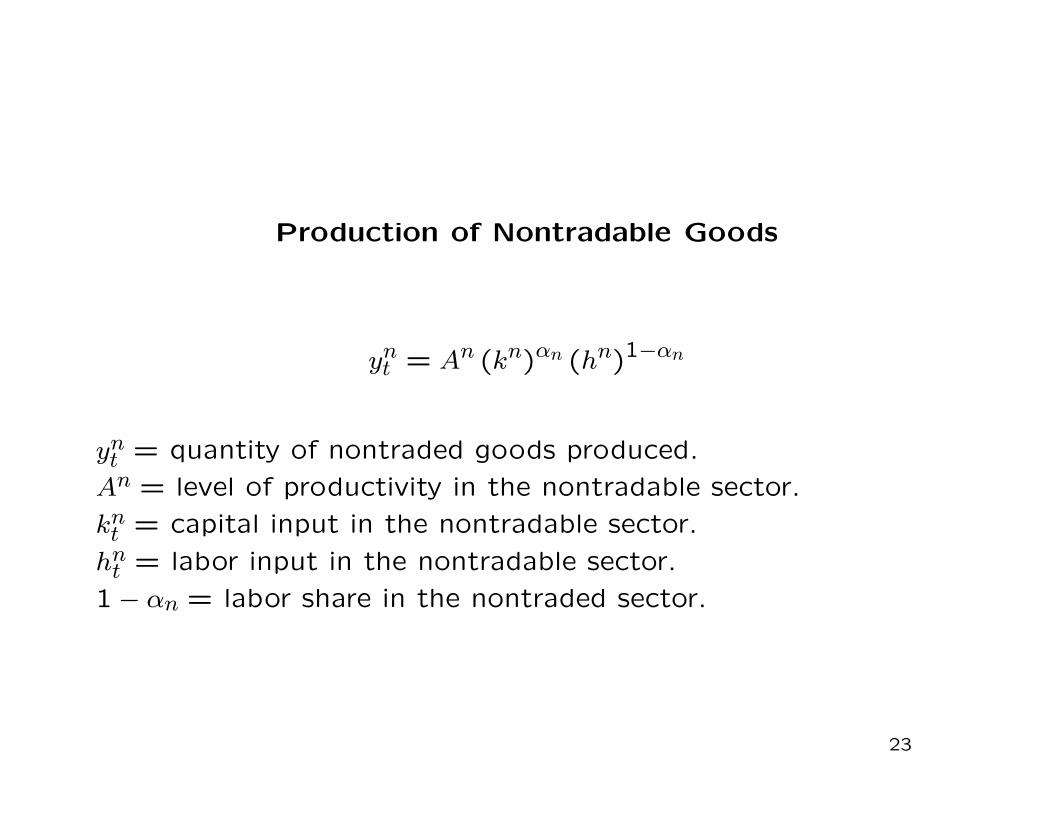
Production of Nontradable Goods
ynt = An (kn)αn (hn)1−αn
ynt = quantity of nontraded goods produced.
An = level of productivity in the nontradable sector.
knt = capital input in the nontradable sector.
hnt = labor input in the nontradable sector.
1 − αn = labor share in the nontraded sector.
23

To ensure a stationary equilibrium process for external debt, we
assume that the country interest-rate premium is debt elastic,
rt = r∗ + p(dt+1)
24

Terms of Trade Process
ln
(tott
tot
)= ρ ln
(tott−1
tot
)+ σtotε
tott ; εtott ∼ (0,1)
tot > 0.
ρ ∈ (−1,1).
σtot > 0.
25

Functional Form Assumptions
p(d) = ψ(ed−d− 1
)
Φj(x) =φj
2x2; j = m,x, n
26

Calibrated and Estimated Parameters
Calibrated Structural Parametersρ σtot αm, αx αn ωm, ωx, ωn µmx µτn tot Am, An β σ δ r∗
∗ ∗ 0.35 0.25 1.455 1 0.5 1 1 1/(1 + r∗) 2 0.1 0.11Moment Restrictionsσiσy
σtbσy
σim+ix
σinsn sx stb
pmym
pxyx
∗ ∗ 1.5 0.5 0.2 0.01 1Implied Structural Parameter Values
φm φx φn ψ χm χτ d Ax β∗ ∗ ∗ ∗ 0.8980 0.4360 0.0078 1 0.9009
Notes.
∗Country-specific estimates.
σiσy
and σtbσy
are conditional on tot shocks
sn ≡ pnyn/y,
sx ≡ x/y,
stb ≡ (x−m)/y, where y ≡ pmym + pxyx + pnyn.
27

Key parameters determining the importance of terms of trade
shocks:
• ρ and σtot, the more volatile and the more persistent are terms
of trade shocks, the more volatile is output.
• The size of the nontraded sector: pnyn
y (= 50%). The larger the
nontraded sector, the smaller the output effects of tot shocks.
• The steady-state trade share: x+my (= 39%). The larger the
trade share, the larger the output effects of tot shocks.
28

Estimate capital adjustment cost parameters and the debt elasticity
of the interest rate, φm, φx, φn, ψ, χm, to match country-by-
country the relative standard deviations
σi/σy and σtb/σy
conditional on terms of trade shocks and σix+im/σin = 1.5.
29

Medians of Country-Specific Estimates of the Capital Adjustment
Cost Parameters and the Debt Elasticity of the Interest Rate
σi/σy σtb/σyφm φx φn ψ Data Model Data Model
Median 1.13 1.40 0.69 0.84 3.36 3.00 0.64 0.74MAD 1.13 1.40 0.69 0.77 1.42 0.52 0.33 0.34
30

Median of Country-Specific Predicted Impulse Response to a Ten-Percent Terms-of-Trade Shock
0 5 100
5
10Terms of Trade
0 5 10−2
−1.5
−1
−0.5
0RER
0 5 100
0.5
1
1.5
2p
N
0 5 10−0.5
0
0.5
1
1.5Trade Balance
0 5 100
5
10
15Imports
0 5 100
2
4
6Exports
0 5 100
0.5
1
1.5
2GDP
0 5 100
0.5
1Consumption
0 5 100
1
2
3
4Investment
0 5 10−4
−2
0
2y
M
0 5 100
2
4
6
8y
X
0 5 100.5
1
1.5
2y
N
0 5 10−60
−40
−20
0
20iM
0 5 10−50
0
50
100iX
0 5 100
2
4
6iN
31

Observations of the figure:
• Substitution effect of an increase in tott on supply side. Firms producemore exportables and less importables, and given pnt would produce lessnontradables.
• Substitution effect of an increase in tott on demand side. Demandfor importable goods and nontraded goods rises, domestic demand forexportable goods falls. Wealth effect is positive increasing the demandfor all goods. Price of nontradables, pnt , rises and the real exchange rateappreciates.
• Both exports and imports increase. Net effect on trade balance turnsout to be positive. Thus model impulse response is consistent withHarberger-Laursen-Metzler effect.
• Aggregate investment increases by less than 10% on impact. But investmentin the exportable sector rises by 61% while in decreases by over 40% inthe importable sector.
32

Variance Decomposition:
We construct the counterpart to the observable variable ‘GDP
at constant LCU’ in the theoretical model as:
yconstant pricest = pxssy
xt + pmssy
mt + pnssy
nt ,
where piss denotes the steady-state price of good i = x,m, n.
In the theoretical model, we deflate consumption and investment
by the GDP deflator (constructed as a Paasche index):
Pt =pxt y
xt + pmt y
mt + pnt y
nt
pxssyxt + pmssy
mt + pnssy
nt
33

Finding:
The median share of the variance of output explained by tot
shocks, according to the 38 calibrated models is 13 percent.
This number is close to the SVAR results but far from the
conventional wisdom.
34

Median Share of Variance Explained by Terms of Trade Shocks
tb y c i RERTheoretical Model 21 13 18 11 1SVAR Model 12 10 9 10 14
35

Cross Country Variation in the Share of Variance Explained
by Terms of Trade Shocks in the Theoretical Model
tot tb y c i RERCross-country Median 100 21 13 18 11 1Median Absolute Deviation 0 13 8 12 6 1
36

Evaluating The Conventional WisdomHow Does the Model Fit Country-Level Data?
0 10 20 30 40 50 600
10
20
30
40
50
60
Alg
Arg
Bol
Bot
Bra
Bur
Cam
Cen
Col
Con
Cos
Cot
Dom
Egy
El
Gha
Gua
Hon
Ind
Ind
Jor
Ken
Kor
Mad
Mal
Mau
Mex
Mor
Pak
Par
Per
Phi
Sen
Sou
Sud
Tha
Tur
Uru
Alg
Arg
Bol
Bot
Bra
Bur
Cam
Cen
Col
Con
Cos
Cot
Dom
Egy
El
Gha
Gua
Hon
Ind
Ind
Jor
Ken
Kor
Mad
Mal
Mau
Mex
Mor
Pak
Par
Per
Phi
Sen
Sou
Sud
Tha
Tur
Uru
Data
Mo
de
l
Share of Output Variance Due to ToT Shocks
The RBC framework appears to have difficulty capturing the
propagation of TOT shocks.
37

Variance of Consumption, Investment, the Trade Balance, and the Real Exchange Rate
Explained By Terms-of-Trade Shocks: SVAR Versus Model
0 20 40 600
10
20
30
40
50
60Consumption
SVAR Model
Theore
tical M
odel
0 20 40 600
10
20
30
40
50
60Investment
SVAR Model
Theore
tical M
odel
0 20 40 600
10
20
30
40
50
60Real Exchange Rate
SVAR Model
Theore
tical M
odel
0 20 40 600
10
20
30
40
50
60Trade Balance
SVAR Model
Theore
tical M
odel
38

Conclusion
1. Conventional wisdom has it that terms of trade shocks represent
a major source of fluctuations for emerging countries.
2. Using SVAR analysis, the present study finds a modest role
for TOT shocks.
3. The analysis suggests that the theoretical framework on which
the conventional wisdom is based, an open economy version
of the RBC model, fails to capture well the transmission
mechanism of TOT shocks at the country level.
39

Extras
40

Model Predictions Using the Median ToT Process
and Matching Median Momentsφm φx φn ψ ρ σtot0.00 41.16 0.37 1.56 0.52 0.08
Share of Variance Explained by Terms of Trade Shocks
tb y c i RERSVAR Model 12 10 9 10 14Theoretical Model 24 19 15 13 0
41

tott = a11tott−1 + π11ε1t ; ε1t ∼ (0,1)
Table 1: The Terms of
Trade Process: Country-by-
Country Estimates
Country a11 π11 R2
Algeria 0.43 0.20 0.18Argentina 0.41 0.08 0.19Bolivia 0.52 0.08 0.29Botswana 0.52 0.06 0.33Brazil 0.53 0.08 0.31Burundi 0.59 0.17 0.34Cameroon -0.05 0.13 0.00Central African Republic 0.86 0.09 0.71Colombia 0.29 0.08 0.08Congo, Dem. Rep. 0.41 0.14 0.17Costa Rica 0.53 0.07 0.30
(continued on next page)
42

Table 1 (continued from previous page)
Country a11 π11 R2
Cote d’Ivoire 0.46 0.16 0.22Dominican Republic 0.44 0.09 0.19Egypt, Arab Rep. 0.70 0.09 0.50El Salvador 0.32 0.13 0.12Ghana 0.17 0.09 0.03Guatemala -0.43 0.11 0.19Honduras 0.55 0.10 0.32India 0.63 0.09 0.38Indonesia 0.55 0.11 0.30Jordan 0.48 0.08 0.22Kenya 0.66 0.07 0.52Korea, Rep. 0.69 0.05 0.41Madagascar 0.65 0.09 0.43Malaysia 0.51 0.05 0.27Mauritius 0.57 0.05 0.40Mexico 0.78 0.09 0.60Morocco 0.41 0.06 0.17
(continued on next page)

Table 1 (continued from previous page)
Country a11 π11 R2
Pakistan 0.61 0.08 0.39Paraguay 0.40 0.12 0.15Peru 0.52 0.08 0.27Philippines 0.53 0.08 0.35Senegal 0.75 0.09 0.50South Africa 0.74 0.04 0.53Sudan 0.61 0.09 0.40Thailand 0.55 0.04 0.34Turkey 0.32 0.05 0.11Uruguay 0.39 0.07 0.19
Median 0.52 0.08 0.30MAD 0.11 0.01 0.11

Table 2: Share of Variance
Explained by Terms of
Trade Shocks: Country-
Level SVAR Evidence
Country tot tb y c i RERAlgeria 100 67 8 58 10 25Argentina 100 28 22 14 16 33Bolivia 100 6 6 8 11 6Botswana 100 20 50 32 32 8Brazil 100 47 16 4 28 57Burundi 100 4 2 4 1 9Cameroon 100 9 14 13 13 16Central African Republic 100 37 6 14 13 53Colombia 100 7 18 7 13 13Congo, Dem. Rep. 100 3 1 1 7 12Costa Rica 100 17 3 1 2 2Cote d’Ivoire 100 30 43 36 43 70
(continued on next page)
43

Table 2 (continued from previous page)
Country tot tb y c i RERDominican Republic 100 20 17 16 28 14Egypt, Arab Rep. 100 62 58 46 65 48El Salvador 100 8 2 4 4 22Ghana 100 4 4 3 3 4Guatemala 100 5 1 2 2 13Honduras 100 7 5 1 7 15India 100 4 13 19 1 1Indonesia 100 13 22 17 23 14Jordan 100 31 13 32 4 5Kenya 100 6 4 9 12 2Korea, Rep. 100 17 2 3 28 36Madagascar 100 7 8 1 3 6Malaysia 100 6 5 3 5 1Mauritius 100 9 2 6 2 4Mexico 100 12 17 12 10 28Morocco 100 2 2 2 3 10Pakistan 100 2 7 2 1 3
(continued on next page)
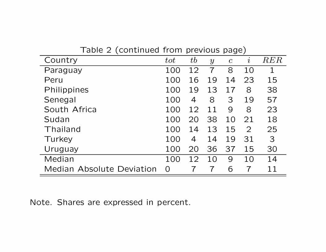
Table 2 (continued from previous page)
Country tot tb y c i RERParaguay 100 12 7 8 10 1Peru 100 16 19 14 23 15Philippines 100 19 13 17 8 38Senegal 100 4 8 3 19 57South Africa 100 12 11 9 8 23Sudan 100 20 38 10 21 18Thailand 100 14 13 15 2 25Turkey 100 4 14 19 31 3Uruguay 100 20 36 37 15 30
Median 100 12 10 9 10 14Median Absolute Deviation 0 7 7 6 7 11
Note. Shares are expressed in percent.

Table 3: Country-Specific Estimates ofthe Capital Adjustment Cost Parametersand the Debt Elasticity of the InterestRate
σi/σy σtb/σyCountry φm φx φn ψ Data Model Data ModelAlgeria 0.01 60.49 32.27 0.01 2.79 6.36 2.10 4.66Argentina 0.55 4.87 1.03 3.33 2.01 2.37 0.36 0.52Bolivia 0.00 76.88 0.00 1.07 4.28 3.32 0.78 0.78Botswana 12.66 0.00 0.00 0.12 5.93 4.45 1.62 1.62Brazil 0.00 108.63 0.00 4.34 3.24 2.72 0.48 0.48Burundi 15.36 0.00 0.04 0.09 2.52 4.23 0.90 1.71Cameroon 0.98 1.07 9.33 84.41 2.14 3.11 0.10 0.15Central African Republic 87.13 0.02 31.60 0.03 7.78 2.92 1.65 1.65Colombia 0.00 47.58 0.00 16.10 3.09 2.56 0.39 0.39Congo, Dem. Rep. 0.00 22.96 0.00 16.82 8.18 2.45 0.30 0.30Costa Rica 12.54 1.06 2.39 0.12 3.05 3.08 1.50 1.50Cote d’Ivoire 0.00 16.81 0.00 16.65 3.37 2.40 0.27 0.27Dominican Republic 0.95 63.29 1.62 7.67 2.86 2.44 0.41 0.41Egypt, Arab Rep. 129.27 0.00 44.73 0.14 5.74 3.37 0.97 0.97El Salvador 0.08 68.21 1.15 6.07 3.35 2.88 0.60 0.60Ghana 0.00 76.88 0.00 3.49 9.55 3.59 0.91 0.91Guatemala 1.28 0.05 1.71 3.10 9.28 9.15 1.81 2.06Honduras 15.51 0.00 0.00 0.29 6.02 3.42 1.09 1.09India 0.30 2.05 0.76 0.97 1.49 1.54 0.27 0.39Indonesia 0.00 41.24 0.00 10.21 4.26 2.37 0.30 0.30Jordan 2.88 2.88 0.62 0.03 1.04 3.40 1.30 2.65Kenya 143.99 0.00 114.22 0.28 5.17 3.07 0.71 0.71Korea, Rep. 133.26 0.00 63.34 0.15 4.86 3.36 0.95 0.95Madagascar 47.35 0.17 0.00 0.28 2.61 2.91 0.85 0.84Malaysia 12.13 0.05 0.05 0.09 4.39 4.67 1.68 1.82
(continued on next page)
44

Table 3 (continued from previous page)σi/σy σtb/σy
Country φm φx φn ψ Data Model Data ModelMauritius 13.07 0.01 0.13 0.05 4.25 4.71 2.34 2.26Mexico 7.56 1.01 0.61 0.24 1.58 1.61 0.40 0.60Morocco 0.00 116.29 0.00 3.25 5.03 3.15 0.67 0.67Pakistan 23.32 0.00 0.00 0.20 8.43 3.48 1.16 1.16Paraguay 0.00 10.68 4.50 0.72 2.13 3.45 0.62 1.02Peru 0.25 14.39 2.61 9.82 2.21 2.27 0.20 0.28Philippines 0.10 8.17 1.11 1.12 1.78 2.43 0.44 0.61Senegal 104.65 0.00 57.74 0.16 14.21 3.22 0.86 0.86South Africa 122.76 0.01 56.35 0.68 2.47 2.63 0.28 0.40Sudan 98.98 0.00 0.00 0.96 4.14 2.41 0.45 0.45Thailand 1.74 1.74 1.32 0.30 0.74 1.62 0.61 0.97Turkey 0.00 16.91 0.00 20.02 6.29 2.50 0.31 0.31Uruguay 0.40 0.40 2.05 4.72 1.70 2.04 0.27 0.42Median 1.13 1.40 0.69 0.84 3.36 3.00 0.64 0.74Median Absolute Deviation 1.13 1.40 0.69 0.77 1.42 0.52 0.33 0.34

Table 4: Share of Variance Explained byTerms of Trade Shocks: Country LevelPredictions of the Theoretical and SVARModels
tb y c i rerCountry TH SVAR TH SVAR TH SVAR TH SVAR TH SVARAlgeria 635 67 16 8 410 58 95 10 3 25Argentina 17 28 6 22 6 14 6 16 0 33Bolivia 16 6 16 6 30 8 19 11 0 6Botswana 2 20 6 50 1 32 2 32 1 8Brazil 54 47 19 16 13 4 23 28 0 57Burundi 65 4 10 2 39 4 7 1 6 9Cameroon 2 9 2 14 2 13 3 13 2 16CAR 920 37 149 6 308 14 44 13 11 53Colombia 9 7 22 18 31 7 11 13 0 13Congo 11 3 4 1 4 1 2 7 1 12Costa Rica 56 17 10 3 30 1 7 2 2 2Cote d’Ivoire 17 30 23 43 27 36 12 43 2 70Dom Rep 10 20 8 17 7 16 10 28 0 14Egypt 33 62 31 58 61 46 12 65 1 48El Salvador 102 8 27 2 25 4 39 4 3 22Ghana 16 4 14 4 8 3 2 3 0 4Guatemala 352 5 30 1 14 2 136 2 0 13Honduras 48 7 37 5 20 1 16 7 1 15India 104 4 161 13 236 19 18 1 1 1Indonesia 20 13 34 22 19 17 11 23 1 14Jordan 23 31 2 13 10 32 7 4 2 5Kenya 29 6 19 4 33 9 19 12 3 2Korea, Rep. 22 17 2 2 4 3 17 28 1 36Madagascar 28 7 30 8 87 1 13 3 3 6Malaysia 6 6 4 5 10 3 5 5 0 1
(continued on next page)
45

Table 4 (continued from previous page)tb y c i rer
Country TH SVAR TH SVAR TH SVAR TH SVAR TH SVARMauritius 35 9 8 2 63 6 9 2 1 4Mexico 85 12 56 17 197 12 36 10 7 28Morocco 10 2 9 2 6 2 6 3 1 10Pakistan 4 2 15 7 13 2 0 1 2 3Paraguay 58 12 13 7 14 8 48 10 0 1Peru 8 16 5 19 10 14 7 23 0 15Philippines 27 19 10 13 18 17 12 8 1 38Senegal 56 4 126 8 254 3 15 19 3 57South Africa 13 12 6 11 18 9 5 8 1 23Sudan 14 20 27 38 18 10 5 21 0 18Thailand 2 14 1 13 2 15 0 2 0 25Turkey 4 4 13 14 7 19 5 31 0 3Uruguay 12 20 9 36 6 37 5 15 0 30Median 21 12 13 10 18 9 11 10 1 14MAD 13 7 8 7 12 6 6 7 1 11