How Family Status and Social Security Claiming Options Shape Optimal Life Cycle Portfolios

Andreas Hubener, Raimond Maurer, and Olivia S. Mitchell

March 5, 2014

Pension Research Council Working Paper Pension Research Council of the Wharton School, University of Pennsylvania

3620 Locust Walk, St 3000 SH-DH Philadelphia, OPA 19104

http://www.pensionresearchcouncil.org                      

The research reported herein was performed pursuant to a grant from the U.S. Social Security Administration to the Michigan Retirement Research Center as part of the Retirement Research Consortium. Additional research support was provided by the Deutsche Forschungsgemeinschaft, the German Investment and Asset Management Association (BVI), the Pension Research Council/Boettner Center at The Wharton School of the University of Pennsylvania, the Metzler Exchange Professor program, and the Eunice Shriver Kennedy National Institute of Child Health and Development Population Research Infrastructure Program R24 HD-044964-10 at the University of Pennsylvania. The authors thank David Love, Sita Slavov, Karen Smith, and John Shoven for generously sharing data and computer code; Yong Yu for excellent programming assistance; and James Anderson for research assistance. Opinions and errors are solely those of the authors and not of the institutions with whom the authors are affiliated. © 2014 Hubener, Maurer, and Mitchell. All rights reserved.

 

 

How Family Status and Social Security Claiming Options Shape Optimal Life Cycle Portfolios

Abstract

This paper investigates how demographic shocks – marriage, divorce, widowhood, and children – along with complex financial options arising from Social Security benefit claiming rules affect optimal household decisions about saving, asset allocation, insurance, and work patterns. In line with empirical evidence, the model predicts stable equity fractions and earlier claiming by wives versus husbands and single women; life insurance is mainly purchased by men. Policy simulations show that Social Security benefit changes will alter work more than financial outcomes. Andreas Hubener Finance Department Goethe University of Frankfurt Grueneburgplatz 1 (Uni-PF. H 23) 60323 Frankfurt am Main, Germany hubener@finance.uni-frankfurt.de Raimond Maurer Finance Department Goethe University of Frankfurt Grueneburgplatz 1 (Uni-PF. H 23) 60323 Frankfurt am Main, Germany maurer@finance.uni-frankfurt.de Olivia S. Mitchell The Wharton School, University of Pennsylvania and NBER 3620 Locust Walk, 3000 SH-DH Philadelphia, PA 19104 mitchelo@wharton.upenn.edu

1  

 

How Family Status and Social Security Claiming Options Shape Optimal Life Cycle Portfolios

1. Introduction

Two crucial factors drive households’ optimal life cycle saving and investment

decisions: labor market work and family status. This is because decisions about hours of work

as well as retirement shape labor earnings, which in turn influence how people spend, save,

invest, and build up retirement benefits through the Social Security system. Not only are

wages uncertain, but so too is family status due to marriage/divorce, the arrival/departure of

children, and spousal death. Each of these poses risks to the household’s financial position:

for instance, the arrival of children changes both household spending and saving patterns due

to higher consumption needs, college costs, and child support in the case of marital

dissolution (Love, 2010). Not only do children influence finances directly; they also change

the amount of time that household members, especially mothers, can work to earn income

essential to build up financial assets (Kimmel and Connelly, 2007).

Also central to life cycle decisions is the role of the Social Security system. In the

United States, this is a national mandatory deferred life annuity scheme with complex

claiming options and cash-flow patterns that depend on age, work history, and family status.

Social Security is especially crucial because it represents such a large component of

household assets. For example, the median Baby Boomer household on the verge of

retirement has accumulated $600,000, of which 40 percent is comprised of Social Security

wealth; the remainder is divided evenly between home equity, non-pension financial assets,

and pension wealth.1 The risk and return profile of the Social Security asset should therefore

have important consequences for how households manage their financial wealth, both during

their worklives and in retirement. Moreover, it is increasingly becoming clear that when to

exercise the option to claim Social Security benefits is one of the most crucial and complex

financial decisions facing workers. For example, claiming benefits at age 70 instead of age 62

boosts lifelong payments by 76 percent (Myers, 1985). Also the financial decision of when to

claim Social Security benefits is different from, although related to, the decision about when

to leave the labor force (c.f., Coile et al., 2002). For example, workers can retire early at age

62, delay claiming until age 70 to earn higher deferred benefits, and draw down financial

                                                            1 This measure (in $2010) includes financial assets, home equity, business and pension assets, and Social Security benefits, and it nets out financial and mortgage debt (see Gustman et al., 2010).  

2  

 

assets to maintain consumption. Or they could claim at the earliest possible age, 62, by

accepting lower benefits but continuing to work, and concurrently receive income from work

and Social Security benefits.

The Social Security system also includes a complex set of rules regarding family

benefits that shape optimal financial wealth and claiming patterns. For instance, couples build

up entitlements to their own old age retirement benefits over their worklives, along with

spousal and widow(er) benefits that depend on the partners’ work histories. Moreover, Social

Security rules permit individuals to first claim old age benefits on their own work records, and

later switch to spousal/widow benefits. In other words, the decision about when to claim

benefits depends intimately on family status; in turn, the claiming age has a large effect on

payouts to spouses and survivors. For these reasons, family benefits can have a pronounced

effect on saving and investment decisions including the demand for risky stocks and life

insurance products. Accordingly, theoretical analysis of the claiming dynamics and the

influence of Social Security benefits on financial wealth management requires examining a

full household optimization framework over the complete life cycle, jointly modeling work,

saving, investment, and claiming decisions. Until now, such a rich and detailed model has not

been available in the literature.

The present paper is the first to incorporate all of these key elements of the household

life cycle – Social Security benefits and family dynamics including children – in a

realistically-calibrated portfolio and consumption choice life cycle model in discrete time with

forward-looking rational multi-person households. We allow for risky asset returns as well as

uncertainty in family status, mortality, labor income, and retirement income. Using data from

the Panel Study of Income Dynamics (PSID), we calibrate wage rate dynamics by age, sex,

education, and family status. In addition, we calibrate the impact of child care needs on

household time using the American Time Use Survey (ATUS). We track individual work

histories for each person separately, and we realistically model Social Security benefits with

spousal and survivor benefits as well as delayed claiming options. In this environment, people

make decisions about saving, investment (stocks/bonds/life insurance products), work hours,

and benefit claiming.

We show that family status has a powerful impact on investment and claiming

decisions. Couples with children invest less in risky assets and purchase much more life

insurance than childless couples or singles. Also, married women claim their own Social

Security benefits much earlier than single women, while married men claim much later.

Interestingly, children have little impact on claiming decisions. These predictions from our

3  

 

theoretical model are consistent with empirical evidence in the Health and Retirement Study

(HRS). Policy simulations confirm that changing Social Security benefits can have a strong

influence on household wealth management and work patterns. For instance, eliminating

survivor benefits would substantially increase women’s claiming ages, by 4 years on average,

while men would claim a year earlier. It would also lead to much higher life insurance

demand for men, with few consequences for household allocations to risky stocks.

Our research builds on and extends the literature initiated by Merton (1969) on life

cycle consumption and portfolio choice models. Recent research has sought to make those

models more realistic by introducing new sources of risk,2 important non-financial assets,3

and endogeneity of labor supply or retirement ages.4 Nevertheless, most of these took the

perspective of an individual representative agent, rather than examining the possibly differing

perspectives of households of varying sizes and compositions. Love’s (2010) work is an

important and invaluable exception, as his was the first model5 to incorporate the effect of

family and marital status risk on portfolio and saving choice. Drawing on PSID data and the

Urban Institute’s Model of Income in the Near Term (MINT), he fitted family transition

probabilities, housing cost processes, and labor income paths that depended on age, sex,

marital status, and children. His main results were that children lead to less accumulation of

financial assets when living at home, and households with children have substantially higher

demand for term life insurance than singles. Nevertheless, that important study was silent on

the likely impact of endogenous labor supply and retirement age on optimal household

patterns, taking account of Social Security rules. By contrast, our more realistic formulation

of Social Security benefit options departs rather dramatically from prior work which assumes

that retirement benefits are simply a fixed fraction of labor earnings as of a pre-specified date.

And our more general approach also permits us to evaluate potential policy reforms including

changes in Social Security rules.

Other papers related to ours in the household finance literature include Shoven and

Slavov (2012) and Coile et al. (2002), both of which explored benefit claiming options under

U.S. Social Security system rules. Using a structural estimation model, Gustman and

Steinmeier (2005) analyzed how retirement and claiming patterns responded to Social

                                                            2 For example, non-tradable risk labor income by Viceira (2001) and Cocco et al. (2005), interest rate risk by Campbell and Viceira (2001), health risk by French (2005), and risk on housing expenditures by Gomes and Michaelides (2005). 3 For example, housing wealth by Cocco (2005), life annuities by Horneff et al. (2008) and Inkmann et al. (2011). 4  See Bodie et al. (1992), Farhi and Panageas (2007), Gomes at al. (2008), and Chai et al. (2011). 5 Earlier work by Scholz et al. (2006, 2007) explored the impact of children on wealth accumulations within a life cycle framework, but it assumed exogenous labor supply/retirement dates and excluded portfolio choice decisions.

4  

 

Security incentives. Yet those studies did not integrate the portfolio choice problem within a

household lifetime optimization framework. Hubener et al. (2013) developed a multi-person

portfolio choice model, allowing for investments in risky stocks, annuities, and life insurance

purchases. Once again, however, that paper focused on retired couples and said nothing about

the work life issue; it also included a simple Social Security benefit rule rather than the more

realistic one we examine here.

In what follows, Section 2 develops the structure of the life cycle portfolio choice

model for households with uncertain family status, time budget constraints that depend on the

arrival and presence of children of various ages, and realistic Social Security benefit options.

Section 3 presents the parameter calibration, most importantly the impact of children on

available time for work and the dynamics of uncertain wage rates. In Section 4, we discuss the

main findings from the model simulations and compare our model predictions about claiming

with empirical evidence from HRS data. Section 5 explores possible policy reforms like

changes in benefit structures under Social Security rules. A final Section concludes and

summarizes results.

2. The Life Cycle Optimization Model

In our model, agents face the risk of exogenous family transitions throughout their

working lives and into retirement. In the following, ( ) denotes a woman (man). Time

0,… , is measured in years. At time 0 (assuming age 20 for women and 24 for

men), the individual starts working life as either single or married; we assume that the four-

year age difference between spouses is fixed over the life cycle. Each individual has an

uncertain life span and may live for a maximum of 80 years.

2.1 Family dynamics

The state variable family is modeled at each point in time as a Markov chain with

35 discrete states. Before retirement, the possible family states are never married, married

couple, divorced, and widowed. We further differentiate each of these states for the woman

and man. In addition, a household can have between zero and three children. We do not

distinguish between never married, divorced, and widowed single retirees. Possible retirement

states for couples include only the wife being retired, only the husband being retired, and both

spouses being retired. When modeling spousal benefits, it is also necessary to differentiate

these states with respect to the age when the husband claimed his own retirement benefits (see

section 2.5). A complete list of all possible family states is given in Appendix A.

5  

 

The time-dependent transition matrix Π , | for this

Markov chain is influenced by five factors: mortality, marriage, divorce, fertility, and children

leaving the household. We abstract from multiple births and divorces during retirement. We

only allow married couples to receive children, and we treat three or more children as the

same family state.6 In the case of a divorce, children are assumed to stay with their mothers.7

At the end of our projection horizon (age 100 for women and 104 for men), we set the

survival probability to zero. In the following, we describe the model for couples and refer to

the single case only when it is not a straightforward simplification of ignoring the absent

partner.

2.2 Financial products

Individuals may select from three different financial products to manage their liquid

wealth: riskless bonds, risky stocks, and term life insurance. Bonds are characterized by a

constant annual real gross rate of return . The distribution of the stock return is assumed

to be lognormal and serially independent.

Each period the individual , may purchase a one-year term life insurance

contract. If the insured person dies within the period , 1 , any surviving spouse or

children receive the face value at time 1. If the insured person survives, no payments

are distributed, since no cash value is built up by the insurance contract. According to the

actuarial principle of equivalence, the premium charged by the insurance company equals

the present value of the expected payout plus some expense loadings , which is given by

1 ⋅ 1 ⋅ . (1)

Here denotes the probability from a mortality table that individual conditional on being

alive at time survives to time 1. The (age-dependent) loading factor reflects expenses

covered by the insurance company for administration and to control for adverse selection.8

2.3 Time budget

Each individual has an available time budget Θ. Depending on family status and age, a

certain amount of time must be spent on child care , . Before retirement, the worker can

decide how much of his available time he will spend in the paid labor market to generate

                                                            6 This limits computational effort. Moreover, the marginal effects of an additional child regarding consumption scaling or child care time decrease with the number of children. 7 The different number of children for a divorced husband matters only for child support payments and affects the possible family states to which he may switch. 8 Modeling life insurance as multi-year contracts would require at least one more state variable for each additional spouse, which would make the model intractable. See Hubener et al. (2013) for a discussion of how single period life insurance contracts can substitute for longer-running contracts.

6  

 

labor income. Working for pay inflicts (unpaid) commuting time t,trav. Time remaining is

utility-increasing leisure . Accordingly, the time budget equation is given as follows:

Θ , t,trav (2)

2.4 Labor income

Depending on the time devoted to paid work , each agent earns uncertain labor

income specified as follows:

⋅ , ⋅ ⋅ , (3)

Here , denotes the wage rate which depends on sex, age, and family status. The variable

is an independent identically lognormal distributed transitory income shock with mean of one,

and is the permanent component of the wage rate with lognormal shock evolving

according to:

⋅ (4)

Note that, in the case of a couple, the transitory shock as well as the permanent income

component is assumed to affect both spouses identically or, equivalently, both transitory and

permanent shocks are perfectly correlated across partners.9 The permanent income component

(and its shock ) have a mean of one, such that , is the average wage for the given

combination of sex, age, and family state.

2.5 Retirement income

From age 62 onward, each spouse has the possibility of claiming Social Security

retirement benefits, up to age 70 when claiming becomes mandatory. The retirement income

payable to the individual is equal to his Primary Insurance Amount (PIA), which is based on

lifetime earnings with adjustment for early or delayed benefit claiming. The Social Security

retirement benefit is given by:

,ret ⋅ ⋅ ret (5)

with being the adjustment factor for early claiming reduction or delayed retirement credit

(relative to the Full Retirement Age), and ret is a lognormal transitory shock with a mean of

one.

                                                            9 The modeling of different income shocks requires one additional state variable which increases the computational burden of solving the model.

7  

 

In accordance with U.S. practice, the PIA is based on the individual’s earnings history.

Using a concave piece-wise linear function, the PIA is computed from the Average Indexed

Monthly Earnings (AIME), which is the worker’s average monthly labor earnings over his

(wage-appreciation adjusted) best 35 years. To keep the model tractable, we use the PIAs for

each spouse as state variables. To be precise, the state variable after claiming is the benefit

amount, which is the product ⋅ of the PIA and the adjustment factor for early claiming

reduction or delayed retirement credit. Hence we need not treat the claiming age as a different

state variable.10 Further details on how the PIAs are used as state variables can be found in

Appendix C.

After claiming retirement benefits, individuals still have the opportunity to continue

working until age 70. If they do, they are taxed at a rate of 50 cents per dollar earned above

the exempt amount of the retirement earnings test, consistent with the U.S. Social Security

rules.11

After both partners have claimed their retirement benefits, the partner with the lower

retirement income may elect to receive spousal benefits instead of his own benefits. These

amount to 50% of the partner’s benefits, unless the spousal benefits are claimed before

reaching Full Retirement Age, whereupon a permanent reduction of up to 30% applies. In

contrast to own retirement benefits, claiming spousal benefits after the Full Retirement Age is

not incentivized with an increase of lifelong payments. Since tracking the claiming age for

spousal benefits requires an additional state variable, our model framework only allows for

claiming spousal benefits at the Full Retirement Age.12 After this age, a partner receives

spousal benefits, if these exceed the own already-claimed old age retirement benefits. Another

rule is that if one partner claims after his Full Retirement Age, the delayed retirement credit

only increases his own benefits, but not his partner’s spousal benefits. In order to exclude the

delayed retirement credit for spousal benefits, we use separate retirement states for different

claiming ages of the husband.13

When a spouse passes away, the surviving spouse may switch to widow(er) benefits.

These are equal to 100% of the deceased spouse’s benefits. In our model, this is not an active

decision; instead, these benefits are automatically paid if the widow(er) benefits are higher. If                                                             10 For a couple, there are 81 possible combinations. 11 Survey evidence shows that most people do understand Social Security benefits are reduced by the earnings test, but most are unaware that their benefits foregone are paid back after the Full Retirement Age; see Brown et al. (2013). Nevertheless, this has been true only since the year 2000. 12 If the spousal benefits exceed the wife’s own benefits at the Full Retirement Age, but she would like to receive benefits from age 62 onwards, she can claim her own benefits at this age, and switch to her spousal benefits four years later. In this way, she can avoid a permanent benefit reduction. 13 Our results suggest that this differentiation is only necessary for husbands, since their retirement benefits are never less than half their wives’ benefits. 

8  

 

retirement benefits have not yet been claimed, the PIA of the surviving spouse is substituted

in place of the PIA of the deceased spouse. Accordingly, we need not track whether the

widow(er)’s PIA results from own work history or that of a deceased spouse.

This quite realistic formulation of Social Security benefit options differs from and

extends substantially the typical approach taken in prior portfolio choice life cycle studies.

That is, the usual approach until now has been to assume that the worker’s retirement benefit

is given by a fixed proportion of his last labor income as of a prespecified date.14 Moreover,

prior studies have not modeled spousal or survivor payments, ignoring the possibility that one

spouse can claim first on her own account, and later switch to alternative benefit payment

streams.

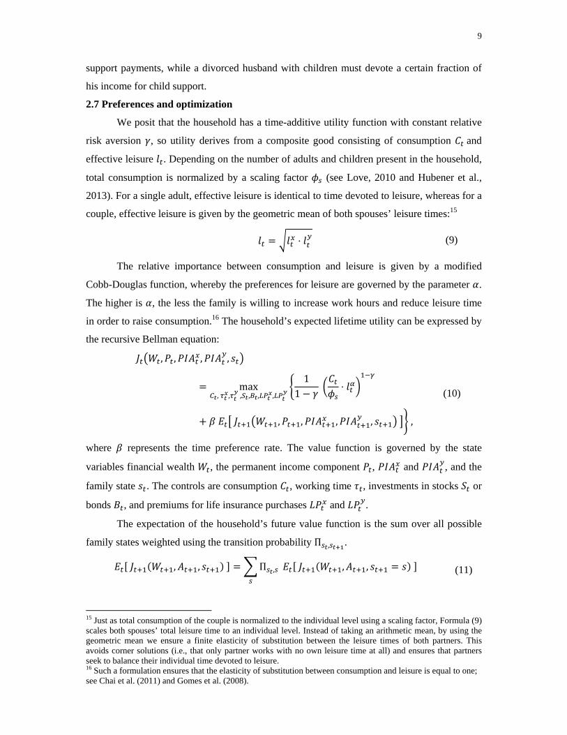
2.6 Wealth dynamics

Besides determining how much time to spend working, each period the household

must also decide how much of its liquid wealth ( ) to spend on consumption ( ), life

insurance premiums for ( , ) for the wife (husband) x (y), and how to allocate savings

to bonds and stocks . The household is liquidity-constrained so it cannot borrow to

finance consumption and life insurance purchases:

(6)

0 0 0 0 (7)

Next period’s liquid wealth is given by any remaining wealth including capital market

returns, labor income ( ), and Social Security benefits ( ,ret), less income taxes according to

proportional rates labor and ret and housing expenses , :

⋅ ⋅ 1 1

⋅ 1 labor,ret ,ret ⋅ 1 ret ⋅ 1 ,

(8)

The indicator variables and are equal to one if the corresponding spouse is alive

at time and zero otherwise. Other cash flows might result due to family state transitions. If

one of the spouses dies, the remaining spouse receives the payment from the life insurance

contract . If a child leaves the household, we assume the parents must pay college fees (here

designed as a lump sum). Furthermore, a divorced woman with children receives child

                                                            14 See for instance Cocco et al. (2005) and Love (2010). Chai et al. (2011) do incorporate a flexible retirement age and a delayed retirement credit, but their study does not track lifetime earnings. Also it takes the perspective of a single representative worker instead of a multi-person household with uncertain family status, as here. 

9  

 

support payments, while a divorced husband with children must devote a certain fraction of

his income for child support.

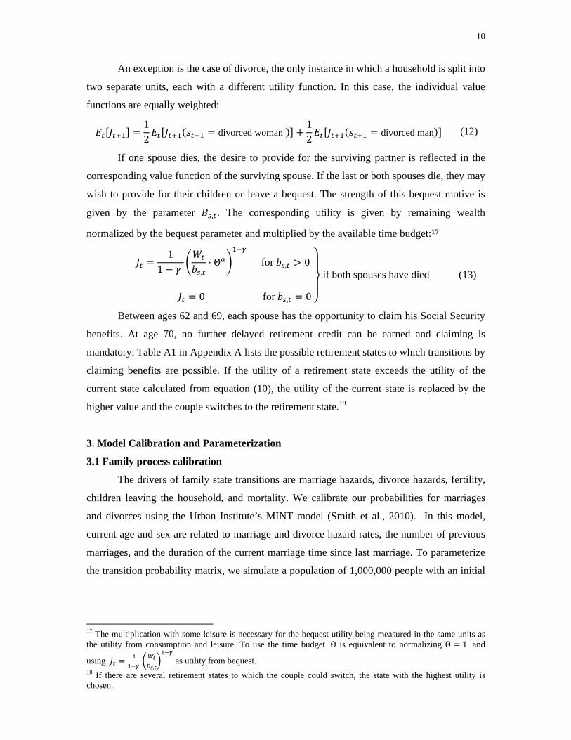
2.7 Preferences and optimization

We posit that the household has a time-additive utility function with constant relative

risk aversion , so utility derives from a composite good consisting of consumption and

effective leisure . Depending on the number of adults and children present in the household,

total consumption is normalized by a scaling factor (see Love, 2010 and Hubener et al.,

2013). For a single adult, effective leisure is identical to time devoted to leisure, whereas for a

couple, effective leisure is given by the geometric mean of both spouses’ leisure times:15

⋅ (9)

The relative importance between consumption and leisure is given by a modified

Cobb-Douglas function, whereby the preferences for leisure are governed by the parameter .

The higher is , the less the family is willing to increase work hours and reduce leisure time

in order to raise consumption.16 The household’s expected lifetime utility can be expressed by

the recursive Bellman equation:

, , , ,

max, , , , , ,

11

⋅

, , , , ,

(10)

where represents the time preference rate. The value function is governed by the state

variables financial wealth , the permanent income component , and , and the

family state . The controls are consumption , working time , investments in stocks or

bonds , and premiums for life insurance purchases and .

The expectation of the household’s future value function is the sum over all possible

family states weighted using the transition probability Π , .

, , Π , , , (11)

                                                            15 Just as total consumption of the couple is normalized to the individual level using a scaling factor, Formula (9) scales both spouses’ total leisure time to an individual level. Instead of taking an arithmetic mean, by using the geometric mean we ensure a finite elasticity of substitution between the leisure times of both partners. This avoids corner solutions (i.e., that only partner works with no own leisure time at all) and ensures that partners seek to balance their individual time devoted to leisure. 16 Such a formulation ensures that the elasticity of substitution between consumption and leisure is equal to one; see Chai et al. (2011) and Gomes et al. (2008).

10  

 

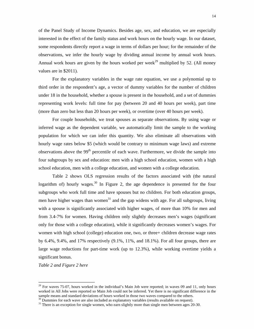
An exception is the case of divorce, the only instance in which a household is split into

two separate units, each with a different utility function. In this case, the individual value

functions are equally weighted:

12

divorced woman 12

divorced man (12)

If one spouse dies, the desire to provide for the surviving partner is reflected in the

corresponding value function of the surviving spouse. If the last or both spouses die, they may

wish to provide for their children or leave a bequest. The strength of this bequest motive is

given by the parameter , . The corresponding utility is given by remaining wealth

normalized by the bequest parameter and multiplied by the available time budget:17

11 ,

⋅ Θ for , 0

0 for , 0

if both spouses have died (13)

Between ages 62 and 69, each spouse has the opportunity to claim his Social Security

benefits. At age 70, no further delayed retirement credit can be earned and claiming is

mandatory. Table A1 in Appendix A lists the possible retirement states to which transitions by

claiming benefits are possible. If the utility of a retirement state exceeds the utility of the

current state calculated from equation (10), the utility of the current state is replaced by the

higher value and the couple switches to the retirement state.18

3. Model Calibration and Parameterization

3.1 Family process calibration

The drivers of family state transitions are marriage hazards, divorce hazards, fertility,

children leaving the household, and mortality. We calibrate our probabilities for marriages

and divorces using the Urban Institute’s MINT model (Smith et al., 2010). In this model,

current age and sex are related to marriage and divorce hazard rates, the number of previous

marriages, and the duration of the current marriage time since last marriage. To parameterize

the transition probability matrix, we simulate a population of 1,000,000 people with an initial

                                                            17 The multiplication with some leisure is necessary for the bequest utility being measured in the same units as the utility from consumption and leisure. To use the time budget Θ is equivalent to normalizing Θ 1 and

using ,

as utility from bequest. 18 If there are several retirement states to which the couple could switch, the state with the highest utility is chosen.

11  

 

marriage rate of 20%,19 for which we track the number and duration of marriages. These then

evolve according to the MINT hazard rates. We derive the transition probability Π , by

dividing the number of transitions in our simulated population from state to state at age

by the number of paths in state . In the MINT model, the number of children does not affect

hazard rates, so these transitions are independent of the number of children. Fertility-driven

transitions probabilities are determined in a subsequent step.

For the transitions between family states with different numbers of children, we use

2009 values of the all-race fertility rates from the National Vital Statistics Reports (Martin et

al., 2011). Reported fertility rates are adjusted for the fact that in our model only married

couples have children.20

We assume that children leave the household when they turn age 18. Since our state

variables track only the numbers of children but not their ages, we again simulate a population

with the already-calibrated fertility, marriage, and divorce transitions, and we track the ages

of the children and have them leave the household after 18 years. The transition probability to

states with one fewer child Π , is given by the number of paths at age with a child turning

18 in state , divided by the total number of paths in state .

Mortality transitions to widow or widower states are given by sex and age-dependent

one-year survival probabilities, for which we use the U.S. 2009 population life table in the

National Vital Statistics Report (Arias, 2014). We assume survival probabilities are

independent of family status.

3.2 Time budget and child care time

Each spouse is assumed to have a time budget of Θ 16 hours per day, and the

possible work week consists of five days (relevant for distinguishing between full, part-time,

and overtime work). We further assume a year to have 52 weeks (relevant for transformation

to annual values) and a month to be 1/12th of a year (relevant for determining the AIME and

PIA).

To calibrate state and age dependent child care time , we use data from 2003-2011

waves of the American Time Use Survey.21 The U.S. Census Bureau conducts the ATUS as

                                                            19 A marriage rate of 20% for 20 year old women and 24 year old men is in line with the MINT study and a bit higher than the National Health Statistics Report (Copen et al., 2012), which reports a marriage rate of 17.3% for women and 11.3% for men age 20-24. But if we add the cohabitation rates (most comparable to the married couple family state) of 18.7% and 15.0%, our assumption is on the low side. 20 The National Vital Statistics Reports give the fertility rate of the complete population tot, the fertility rate of unmarried women , and the fraction of unmarried births to all births. The fertility of married women is then

derived by: tot

.

21 A good description of the ATUS can be found in Hamermesh et al. (2005). 

12  

 

an extension to the Current Population Survey (CPS). Two to five months after households

complete the last CPS interview, they are eligible for the ATUS. One adult per household is

randomly selected to do the interview; this structure precludes us from analyzing empirically

the interaction of couples’ time allocations. The 24-hour time diaries are collected using

telephone interviews, when the respondents report each activity of the previous day and its

corresponding duration. The interviewer assigns each reported activity a code categorized into

17 top-level categories with several sub-categories. After the first wave of 2003, which had

20,720 respondents, there were about 13,000 respondents in each subsequent wave.22

In prior life cycle studies with endogenous labor supply (e.g., Gomes et al., 2008; Chai

et al., 2011), time is divided only into (income-generating) working time versus nonwork. Yet

in that context, nonwork time cannot be viewed as exclusively recreational since it

incorporates both pure leisure and home production (Gronau, 1977). Similar to children’s

effects on consumption, represented in our model by a consumption scaling factor , child

care time , is intended to capture the effect of children on the parents’ time budgets. But

considering only time directly devoted to children would be incomplete, since other activities

may take longer with children present in the household (for example, cleaning the house or

cooking for more people). In this sense, , cannot be viewed as child care alone, but rather it

is the marginal effect of children on all activities related to home production.

Accordingly, for the calibration of , , we consider the following ATUS activities as

home production time: Caring For & Helping Household Members23, Household Activities,

Consumer Purchases, Caring For & Helping Nonhousehold Members, Professional &

Personal Care Services,24 Household Services, Government Services & Civic Service, and all

travel related to those activities.25 We divide the ATUS respondent sample into four

subgroups: married women, married men, single women, and single men, and we drop

observations older than age 66. Next, we include only those observations where the age

difference to the youngest child is at least 18 years and at most 45 (55) years for women

                                                            22 Slightly more than half the diaries are recorded on the weekend or a holiday. 23 This includes all 19 activities related to children like physical care, supervising children’s activities, and playing with them. Even though the latter can be seen as recreational leisure, we choose not to exclude it due to its direct reference to the effect of children on available time. 24 Note that these are the time costs to make use of the service, as for example waiting on a babysitter. 25 We exclude the following activities: Personal Care, Work & Work-Related Activities, Education, Eating & Drinking (without food preparation), Socializing, Relaxing, & Leisure, Sports, Exercise, & Recreation, Religious & Spiritual Activities, and Volunteer Activities. Our model assumes a day has 16 waking hours and hence we exclude personal care, which is mainly sleeping time besides washing, dressing, and grooming. Education is excluded due to its close relation to work and all the other activities are recreational leisure.

13  

 

(men).26 Finally, we exclude the time diaries filled out on holidays or weekends. Naturally,

we include observations with and without children to identify the effect of children. We then

regress time spent on the aforementioned activities on a set of dummies for the number of

children (with one dummy representing three or more children), and a second/third27 order

polynomial in the number of years until the youngest child turns age 18. The estimated OLS

coefficients appear in Table 1, accompanied by a graphical representation of the results in

Figure 1. In general, women allocate more time than men to home production. Also children

boost women’s time devoted to non-market activities more than men’s. Single women do

spend less time on these activities than married women, but the effect of (at least the first two)

children is about the same for both female groups.

Table 1 and Figure 1 here.

For someone with no children, the set of child dummies and the age of the youngest

child are set to zero, so the regression constant term reflects time spent on home production

when no children are present. As mentioned above, , captures only the marginal effect of

children on home production time, so rather than setting , to the estimated home production

time for each family state , we set , to the difference in home production time with

reference to someone having a similar marital status but with no children (e.g., married couple

with two children versus a married couple with no children).

As noted above, our state variables do not directly track the ages of children at home.

Instead, for the calibration of transition probabilities, we simulate a population keeping track

of the children’s ages. For each path, child care time is calculated according to the regression

results,28 and the value , is derived by computing the mean over all paths for corresponding

family state at (parent’s) age .

We also use the ATUS for calibrating the time needed to commute to work. The

sample mean for those who worked at least an hour for pay and travelled to work less than

four hours on the diary day is t,trav 0.64 hours for women and t,trav 0.79 hours for men.

3.3 Wage rate calibration

We estimate the deterministic component of the wage rate process , and the

variances of the permanent and transitory wage shocks and , using the 1975-2011 waves

                                                            26 There is no indicator as to whether the children in the home are the biological children or not. These restrictions should minimize the observations of people looking after their underage siblings and grandparents looking after their grandchildren. 27 For all subgroups except married women, the coefficient of third order in child age is not significantly different from zero so we reduce the order of the polynomial used for them. 28 Since the number of single men with children is small, we use the regression results of single women for widowed men with children. 

14  

 

of the Panel Study of Income Dynamics. Besides age, sex, and education, we are especially

interested in the effect of the family status and work hours on the hourly wage. In our dataset,

some respondents directly report a wage in terms of dollars per hour; for the remainder of the

observations, we infer the hourly wage by dividing annual income by annual work hours.

Annual work hours are given by the hours worked per week29 multiplied by 52. (All money

values are in $2011).

For the explanatory variables in the wage rate equation, we use a polynomial up to

third order in the respondent’s age, a vector of dummy variables for the number of children

under 18 in the household, whether a spouse is present in the household, and a set of dummies

representing work levels: full time for pay (between 20 and 40 hours per week), part time

(more than zero but less than 20 hours per week), or overtime (over 40 hours per week).

For couple households, we treat spouses as separate observations. By using wage or

inferred wage as the dependent variable, we automatically limit the sample to the working

population for which we can infer this quantity. We also eliminate all observations with

hourly wage rates below $5 (which would be contrary to minimum wage laws) and extreme

observations above the 99th percentile of each wave. Furthermore, we divide the sample into

four subgroups by sex and education: men with a high school education, women with a high

school education, men with a college education, and women with a college education.

Table 2 shows OLS regression results of the factors associated with (the natural

logarithm of) hourly wages.30 In Figure 2, the age dependence is presented for the four

subgroups who work full time and have spouses but no children. For both education groups,

men have higher wages than women31 and the gap widens with age. For all subgroups, living

with a spouse is significantly associated with higher wages, of more than 10% for men and

from 3.4-7% for women. Having children only slightly decreases men’s wages (significant

only for those with a college education), while it significantly decreases women’s wages. For

women with high school (college) education one, two, or three+ children decrease wage rates

by 6.4%, 9.4%, and 17% respectively (9.1%, 11%, and 18.1%). For all four groups, there are

large wage reductions for part-time work (up to 12.3%), while working overtime yields a

significant bonus.

Table 2 and Figure 2 here

                                                            29 For waves 75-07, hours worked in the individual’s Main Job were reported; in waves 09 and 11, only hours worked in All Jobs were reported so Main Job could not be inferred. Yet there is no significant difference in the sample means and standard deviations of hours worked in those two waves compared to the others. 30 Dummies for each wave are also included as explanatory variables (results available on request). 31 There is an exception for single women, who earn slightly more than single men between ages 20-30. 

15  

 

For estimating the variances and of shocks to permanent income and , to

transitory income, we follow the well-established procedure of Carroll and Samwick (1997).

The idea is that the residual of the observed log wage in the PSID and the predicted log wage

from our regression results can be attributed to permanent income and transitory shocks

ln ln . Let , ln ln ln ln be the difference of these

residuals of waves for individual , years apart. Under the assumption of serially

uncorrelated and independent shocks, this difference has a variance of 2 . Regressing

the squared differences , on the time span between waves and a constant vector of 2’s

yields an estimate for these variances.

The results of our calibration appear at the bottom of Table 2. Since we assume

identical shocks for both spouses, we split the sample by education but not by sex. Compared

to Love (2010) who based his empirical analysis on a broader definition of household income

(including public transfers and unemployment compensation, as well as labor income), our

estimate of the variance of permanent shocks is about the same for the less educated and

slightly higher for the college educated. Our variance of transitory shocks is considerably

lower for both educational groups. For retirement income, which is purely a public transfer in

our model, these conceptual differences no longer apply. Therefore, for the variance of

transitory shocks to retirement income we set 0.0784 (as in Love, 2010).

3.4 Other parameters

Emulating several other studies in the life cycle literature, we use the household

consumption scaling factors proposed by Citro and Michael (1995), 0.7 ⋅ . ,

with being the number of adults and being the number of children in the household. Our

calibration of bequest strength , is motivated by a provisional motive, that is, to provide for

children’s consumption and education costs. We set , to zero for any family states without

children present which applies to all retirement states, among others. Otherwise, we assume

that an annuity must be purchased that finances the consumption for each left-behind child

until his 18th birthday, plus four years of college.32 As childrens’ ages are not explicitly

tracked in our model, we again use the same simulation technique as before for the family

transition probabilities and child care times to derive mean values of , for family state at

each age .

                                                            32 Abstracting from discounting with the riskless rate, a 15- and a 17-year old child yield bequest factors of

5 ⋅ 0.7 ⋅ 2 . 2 ⋅ 0.7 ⋅ 1 . 7.89, since consumption must be financed for five years for both children and another two years for the youngest child.

16  

 

In our baseline case, we use a relative risk aversion of 5 and set the time discount

factor to 0.96. The leisure preference parameter is given by 0.8, since for this value,

the optimal life cycle profiles for hours worked per week roughly match the average work

hours in the PSID data used for the calibration of the wage rate (also see Appendix B). The

risk-free rate is set to 1.02, and we assume an equity premium for stock returns of

t 4% with a standard deviation of stock returns of 20%. Life insurance contracts

are priced according to the 2001 Commissioners Standard Ordinary (CSO) Mortality Table,

which was developed by the Society of Actuaries and the American Academy of Actuaries

(2002). As in Gomes et al. (2008), labor earnings are taxed at a rate of labor 30% and

retirement benefits at ret 15%.

Several other parameters are calibrated following Love (2010): for instance, we use his

estimation of housing costs , from PSID data; for child support, divorced men are assumed

to pay 17%/25%/30% of their labor income for 1/2/3+ dependent children; divorced women

with children receive the corresponding fraction of a single man’s income as if he works for

40 hours per week; when a child turns age 18, the household pays 40% of its permanent

income resulting from full time work for college costs33 upon his departure; in the case of

divorce, wealth is split evenly between spouses after deducting 10% of assets for divorce

costs.

When a single individual marries, we must make some assumptions about the new

partner. First, we posit that the new partner has the same permanent wage rate component

as the single individual had before marriage. Second, the PIA of the new husband is an age-

dependent multiple of the wife’s PIA, ranging from 1.06 in their early 20’s, to 1.09 just before

retirement. Third, the financial wealth brought by the husband into the couple’s wealth is also

an age-dependent multiple of the wife’s wealth, ranging from 1.08 early on, and 1.12 late in

life.34

When a couple divorces, the partner with lower retirement benefit claims is entitled to

spousal benefits, and after the former partner’s death, to widow(er) benefits. Our model does

not track the PIA of former partners, so we increase the PIA of a divorced woman (man) to

70.85% (58.23%) of the former partner if her (his) own PIA is smaller. This is motivated by

the following consideration: an annuity paying $50 per year to a woman as soon as her former                                                             33 Based on a study by Turley and Desmond (2006), Love assumes college costs of 10% of the family’s income for four years. Since the family states in our model do not contain any information on the number or even the ages of children already having left the household, we have to model this payment as a lump sum upon the child’s leaving.  34 We derive these multiples by assuming that both partners have worked full time up to this age. The ratio of the PIAs resulting from this work history yields the first multiple. Similarly, the second multiple is calculated from the ratio of corresponding average lifetime income.

17  

 

husband reaches full retirement age, and $100 after his death, as long as the woman lives, has

the same actuarially fair present value as an annuity paying the woman $70.85 per year

(because of the age difference and the asymmetry in the mortality rates, the corresponding

value for men is only $58.23).

For the piecewise linear function converting the AIME into the PIA, we use the

official specification for the Social Security bend points. For the first $749 of the AIME, 90

cents per dollar are transferred into the PIA, for values over this and up to $4,517, 32 cents

per dollar are transferred and for every additional dollar earned, on average, the PIA increases

by 15 cents (in $2011). We set the exempt amount of annual income for the Retirement

Earnings test to $14,160.35 The deduction (bonus) for claiming early (late) old age retirement

benefit is calculated according to Social Security claiming rules. As of the Full Retirement

Age, defined here as age 66, retirement benefits as a fraction of the PIA are given by Table 3.

Table 3 here

4. Optimal Decisions on Saving, Work, Claiming, Life Insurance, and Investments

In this section, we first analyze the household’s optimal behavior over the life cycle. In

particular, we are interested in how family status affects financial decisions (stocks, bonds,

life insurance demand), work effort, and the optimal time to exercise the Social Security

claiming option. Next, we discuss the simulation method for the life cycle model with

changing family status. In Section 4.2, we present patterns of average consumption, wealth,

holdings in stocks, work hours, and Social Security claiming ages. We discuss these patterns

for women and men in single and couple households. Further analysis on how education and

the number of children influence optimal decisions appears in Section 4.3. Finally, we

investigate whether the predictions on claiming patterns from our model are consistent with

empirical data.

4.1 Simulations

We use the optimal controls of the baseline parameterization of our life cycle model to

generate 100,000 simulated life cycles reflecting realizations of stock returns, wage rates, and

marital status. We assume that 59.3% (40.7%) of the simulated households have a wage rate

profile corresponding to the high school (college) educated (as in in the 2011 wave of the

PSID). We divide the sample of simulated life cycles equally into female and male paths. At

the start of the simulations, 80% are singles and 20% are already married, while later in life,

each individual randomly moves between the 35 family states. Each household is endowed                                                             35 For additional information on Social Security benefit rules, see Myers (1985) and http://www.socialsecurity.gov/OACT/COLA/rtea.html.

18  

 

with a starting financial wealth as if each household member would have worked 40 hours per

week in the previous period. We present the results in the usual way as in the life cycle

literature, so we generate simulated paths conditional on survival. To do so, we modify the

transition matrix , for the simulation by setting the mortality of women in female paths

and men in male paths to zero36 and rescale the other probabilities such that they sum up to 1.

This procedure keeps the same number of paths even at high ages. If a single agent marries,

we make the same assumptions about the new spouse as in the optimization regarding age

difference, permanent income, wealth, and PIA. In the case of divorce, we follow only the ex-

wife (ex-husband) in a female (male) path and ignore the other spouse.

For the reporting of aggregate quantities over all paths, such as for example average

wealth, each path is weighted with the survival probability to the age in question. This gives

female paths a slightly higher weight in comparison to male paths, especially at older ages.

When sex-dependent quantities like hours worked by women (men) are considered, we only

report the average over female (male) paths. We also report results for subsamples, e.g. single

or couple households. In this case, we use averages over all paths in that family state at the

reported age. Thus the samples are not constant at all different ages. For example, an

individual who is seen to be a single woman at one age will drop out of the single sample

when she marries. She can also reenter the single subsample at a later age, if a divorce occurs.

Table 4 provides some basic information about the average composition of the simulated

population dynamics at different ages.

Table 4 here

4.2 Optimal life cycle profiles

Figure 3 reports the average life cycle profiles for the complete population of singles

and couples with either a high school or a college education. Panel A shows average

consumption, life insurance demand, wealth level, and investments in equities. Panel B

reports average work hours for men and women, and Panel C the frequency of claiming

Social Security benefits. Here we see that financial wealth builds up gradually until age 55

when it amounts to about $189,000 on average, and thereafter people start to draw down their

assets. The average wealth profile generated from our life cycle model is reasonably

consistent with empirical data. For example, in the PSID (see Appendix B), the average

financial wealth of households between age 25 and 75 is about $140,000 (in $2011), while

households in our model have an average wealth of $149,000 in the same age bracket. But in

                                                            36 However, the optimal decisions of the agents take mortality into account. The mortality of the spouses in couple states is not zero and states of widowhood are thus possible in the simulation.

19  

 

our model, the wealth profile is shaped slightly differently, as younger households have

higher and older households have lower wealth in comparison to their empirical counterparts.

Figure 3 here

Levels of financial wealth and how much people invest in risky stocks are highly

correlated. Compared to other papers in the life cycle literature,37 our model generates a

relatively low and stable fraction invested in the stock market. For instance, during the first

decade of the life cycle, stock allocation rises from about 20% at age 20, to 61% at age 35.

Subsequently the average allocation to stocks is quite stable, in a range of 44% to 61%. After

age 62, when households start to claim Social Security benefits and receive their riskless

benefits, the fraction invested in stocks increases slightly, to 54%. There are two reasons for

these low levels of equity exposure. First, adding family status uncertainty on top of

permanent/transitory income and mortality shocks, forces households to select safer bond

investments to cover own and children’s consumption needs, as noted by Love (2010).

Second, the portion of cash-on-hand dedicated to this period’s consumption is assumed to be

held in a transaction account of non-risky assets.38 The portfolio allocation generated by our

life cycle model fits the empirical data quite well. For instance, several studies on U.S.

household portfolio allocations report a relatively constant, non-decreasing equity share by

age conditional on participation, of around 40-60%.39

Our results also show that the average level of consumption increases over the

worklife. Thereafter, consumption drops sharply from about age 66, when many households

retire and begin to consume more leisure. This profile is consistent with other life cycle

models with endogenous work hours and flexible retirement ages (Chai et al., 2011);40 it is

also in line with empirical studies documenting a substantial drop in spending around the

retirement point. Thus Bernheim et al. (2001) and Aguiar and Hurst (2005) report a drop of

consumption expenditures after retirement for U.S. households of 35-38 percent (depending

on wealth levels). Their explanation is that retirees are more willing to increase time for home

production, and concurrently curtail their consumption expenditures. This is in line with our

findings, since home production is a major part of non-labor force time, in our model (see

Section 3.2).

                                                            37 See Cocco et al. (2005), Gomes and Michaelides (2005), Gomes et al. (2008). Love (2010), or Chai et al. (2011). 38 This is in line with recent work by Abel et al. (2013). Drawing on early work by Baumol (1952), that study uses a dynamic consumption and portfolio choice model where a liquid riskless asset is held in a special transaction account to cover consumption expenditures until the next period. 39 See, for example, Guiso et al. (2002), Ameriks and Zeldes (2004), Gomes and Michaelides (2005), Love (2010), and Wachter and Yogo (2010). 40 By contrast, life cycle models with exogenous labor income and retirement age, such as Cocco et al. (2005) and Love (2010), generate a quite smooth average consumption profile before and after working life.

20  

 

Figure 1B shows that men start off with an average of 45 work hours per week which

they gradually reduce to around 40 hours right before the earliest possible retirement age.

Women also work for pay more than 40 hours a week in their early 20’s, but they reduce this

to about 32 hours per week in their late 30’s. Thereafter, they remain at this level until

reaching the earliest retirement age. Compared to empirical data, our model predicts slightly

lower values of work hours with a bigger gap between men and women. (Thus Appendix B

reports average work hours for those age 25 to 55 using PSID data of 45 hours per week for

men, and 38 hours per week for women.) Our model also implies that men will claim Social

Security benefits slightly later than women (Figure 3C). Additionally, their demand for life

insurance is much higher (Figure 3A). To gain more insight into what drives these results, we

turn next to separate analyses of single versus couple households.

Figure 4 presents the expected life cycle profiles for singles. Panel A shows that

wealth builds up gradually until age 58, when it amounts to about four times average

consumption. Thereafter, the singles begin to draw down assets to compensate for fewer hour

of work. Between age 60 and 80, wealth levels are relatively flat (besides a slight bump

around age 66), for two reasons. First, the singles gradually claim their Social Security

benefits between age 62 and 70 but they need not fully leave the labor force. Instead they

work part time up to the earnings test exempt amount. Depending on education, this

corresponds to about 19 hours per week for high school graduates and 14 hours for college

graduates. This explains relatively flat wealth levels up to age 70. Second, though households

do start to decumulate their assets post-age 70, mortality is also rising. For this reason, the

pool of singles is increasingly subject to an influx of widows and widowers holding higher

wealth levels from their coupled state. Accordingly, the transition from couple to single tends

to neutralize the aggregate effect of dissaving, which accounts for the relatively flat overall

wealth levels to age 80.

Figure 4 here

For singles, the share of financial wealth in stocks is relatively constant over the life

cycle (at 40-60%), similar to the overall population. Singles’ average consumption is lower,

but the same overall pattern prevails as in the aggregate. We also see that singles have

virtually no demand for term life insurance; they have no provisional and bequest motives as

generally they have no children or partners to provide for after death (Hubener et al., 2013)

and they gain no (altruistic) utility from the transfer of wealth to the next generation. Only for

single women age 30-40 is there a small positive demand for life insurance; this is generated

by divorced women who must cover their children’s consumption and college education costs

21  

 

should they die young. There is very little life insurance demand among single men, since the

only case for which single men must take care of children is when they are widowers. Since

young women’s mortality is very low, the few such cases do not change average life

insurance demand overall.

Turning to labor supply patterns, Figure 4B shows that single men work for pay 42

hours per week at the beginning of their life cycles. Thereafter, they gradually reduce their

time on the job to 32 hours just before retirement. From age 62 onward, men begin to claim

Social Security benefits which provide them with a safe income stream for life. In conjunction

with the possibility of receiving Social Security benefits and working without tax penalties up

to the earnings test exempt amount, most men reduce their average work hours sharply and

work only part time (to 16-27 hours per week) after claiming. Average paid work hours for

women are lower than for men, since women have, on average, lower wage rates.

Accordingly, they are less willing to curtail their leisure time for higher consumption afforded

by more work. An additional explanation is that the single sample includes divorced women

with children who are financially supported by their ex-husbands and have lower time budgets

due to child care responsibilities. The consequence is that these women work less for pay,

compared to single women without children. This explains the slightly increasing gap of paid

work hours between men and women age 35-45. In this age group, about 30% of single

women have children. From age 45-55, this gender gap decreases, because the children

become older and require less time (or leave home). After age 60, when children are out of the

house, men and women exhibit very similar work patterns.

Panel C of Figure 4 displays Social Security claiming patterns by age. Single women

claim slightly later than their male counterparts: thus the mean claiming age is 65.2 for men

and 66.8 for women, and about 34% (20%) of single men (women) claim Social Security

benefits at the earliest possible age of 62. These households are unwilling to take advantage of

the additional life annuity benefits from delayed claiming. After a claiming peak at age 62,

7% additional singles on average claim their benefits at each subsequent age until 69. More

detailed analysis shows that early claiming households build up relatively low wealth during

their working lives and have low permanent wage rates in their 60’s. Since the replacement

rates under the U.S. Social Security system are progressive, lifetime poor households have

low PIAs receive a higher replacement rate. This enhances their incentives to claim Social

Security benefits early and work part time up to the earnings test exempt amount, to augment

overall income. About 15% (33%) of single men (women) delay claiming to age 70, when

claiming becomes mandatory. On average, these households have a higher permanent wage

22  

 

rate and consequently build up more financial wealth than do poorer, earlier claiming,

households. This later claiming pattern arises because they can take advantage of the

increased real annuity income from the delayed retirement credits. Moreover they take

advantage of still high wage rates and work longer; claiming later avoids the penalty from the

earnings test.

Next we turn to life cycle profiles for couples; Panels A – C in Figure 5 highlight

several important differences compared to singles. Most importantly, wealth and consumption

levels are much higher for couples than singles, due to the fact that couple households have

multiple members. Interestingly, younger couples build up wealth more quickly than singles:

between age 20 and 30, the average level of wealth for couples increases by about 13% per

year, but by only by 8.5% annually for singles. Also, wealth relative to family size is higher

for younger couples: for instance, at age 30 the ratio of average wealth to consumption for

couples is 3.5, but only 2 for singles. This is because of couples’ higher precautionary saving

motives due to uncertainty in family status (divorce, death), as well as having to save for

college education. After the mid 50’s, household wealth peaks and children start to leave the

home, and these differences between singles and couples shrink.

Figure 5 here

Couples’ demand for life insurance is hump-shaped, with insurance purchased mainly

on the husband’s life: average face values peak at around $143,000 at age 37, when most

couples have children and many women reduce their paid work hours substantially because of

childcare demands. Demand for life insurance on the wife’s life is clearly lower than on the

husband’s, topping out at $44,000. One reason is that female mortality is substantially lower

than men’s; another is that men have higher wages than women, so a widower can more easily

provide for the family than can a widow. In addition, the re-marriage rate of widowers with

children is more than twice as high as for widows, so widowers are much more likely to find a

new partner to help with child care and provide a second income. The demand for life

insurance on women age 30-50 is driven by couples with more than two children. In this

instance, the wife’s death would impose a substantial burden on the husband, because he

would need to curtail his work hours to care for the young children. Life insurance purchases

of both partners combined with accumulated liquid savings cover the risk that both parents

might die at once.

Interestingly, the demand for life insurance during retirement is zero for both partners.

Because of generous Social Security widow benefits, retirement income proves to be rather

symmetrically distributed between both partners, so only a minor portion of retirement

23  

 

income is lost when one spouse dies. If the husband dies first, his surviving widow receives

100% of his Social Security benefit as his widow, an amount typically higher than her own

(and her spousal) benefit. In addition, the surviving spouse retains the household’s remaining

liquid wealth, and as a single she requires lower consumption. Therefore the death of one

partner need not cause a large consumption shortfall that would need to be hedged by life

insurance purchases.41

The work hour pattern for couples differs distinctly from that of singles. During their

early 20’s, both husbands and wives work for pay up to 50 hours/week. In contrast to single

men, husbands reduce work to 44 hours around age 40, and they maintain this level until

retirement, effectively working about 5 hours per week more than single men. Wives, on the

other hand, reduce their paid work hours in their late 30’s to about 30/ week. Between age 40-

55, women gradually boost their paid work to 32 hours/week, when children are older and

require less home time. Despite their high work hours at younger ages, wives work for pay

about 3 fewer hours per week over the life cycle, compared to single women. This

specialization of work hours within the family is due to the fact that women’s wage rates are

lower than men’s, on average, and they fall further on the arrival of children. Thus the wife

shoulders most of the unpaid burden of child care and home production time, and she works

less for pay than the husband. Similar to the situation for singles, both husband and wife start

to reduce their market work substantially in their 60’s.

Interestingly, couples’ Social Security claiming patterns differ remarkably from those

of singles. About 55% of married women claim their own old-age Social Security benefits at

the earliest possible age of 62. Their mean claiming age is 64.8, about 2 years earlier than

single women. By contrast, 41% of married men delay claiming up to age 70 and their mean

claiming age of 66.5 is 1.3 years higher than for single men. There are several explanations

for these differences. First, married women’s PIAs are considerably lower than those of their

husbands.42 In addition, married women are eligible for spousal benefits and later to relatively

generous widow benefits (100% of their husbands’ benefits). The Social Security claiming

rules also permit the wife to switch from her own old age retirement benefits to spousal

benefits and/or to widow benefits when the husband passes away. Spousal benefits increase

for every year of delaying after age 62 by about 8% (up to the normal retirement age 66).

                                                            41 This result supports Hubener et al. (2013) who also found no demand for life insurance when the couple’s retirement income flows were symmetrically distributed; that study however did not incorporate retirement patterns. 42 Since our model assumes the same permanent income for both spouses with the husband’s deterministic component being higher and the work hours of women being lower, our simulations do not have any wife with a higher PIA than her husband.

24  

 

Because of these switching possibilities and particularly due to the generous widow benefits,

early claiming for married women only reduces their retirement benefits up to the point of the

husband’s death.43

As a result, for most couples, the optimal strategy to maximize lifetime benefits is for

the wife to claim her relatively lower own benefits early, and to claim spousal benefits later if

they are higher. In addition, the husband will claim his own old age benefits relatively late in

life. This increases his own benefits and also his potential widow’s benefits after his death.

Because of the high probability that the wife outlives her husband, better widow benefits are

important to maximize the couple’s joint lifetime utility.

Such a strategy also effectively hedges longevity risk. If one partner dies, the

surviving spouse receives the high benefits of the husband (either directly or as widow

benefits) for the rest of his or her life. If both spouses survive for a long time, they continue to

receive both incomes, i.e., the own benefit of the husband and the spousal or own benefits of

the wife. Even though the benefits for the wife are smaller, the couple profits from the

consumption scaling of not having to consume twice as much as a single person.

Coincident with the results for single men, married men’s higher permanent wage

rates on average produce later claiming patterns. The few households (some 26%) in which

wives delay claiming to age 70 also have very high wage rates. These high-earning women

seek to remain in the workforce to generate high labor income and take advantage of the

delayed retirement credit by claiming later.

Having seen how married couples specialize, with the husband being the major earner

and wives devoting more time to home production, we revisit the retirement behavior of

single women. These can be categorized in two subgroups: divorced and never married.

Women that never marry have an average claiming age of 66, while divorced women claim

on average 1.1 years later. Being the only one receiving income in a household, never married

women average almost 40 hours/week in paid work. By contrast, divorced women average

                                                            43 The change in the actuarial present value of retirement benefits caused by the timing of claiming is very different for single and married women, as illustrated in the present value calculations by Coile et al. (2002) and Shoven and Slavov (2012). For instance, assume a single woman claiming retirement benefits at age 62 would receive $7500 per year for the rest of her life; this would generate an actuarial present value of $130,224 (at a discount rate 2% and with survival probabilities as in the text). Delaying claiming to age 66 produces higher benefits of $10,000 per year (see Table 3) with a present value 4% higher, of $135,367, computed as of age 62. By contrast, a married woman’s benefits consist of two portions: her own old age benefits (or spousal benefits if greater), and her widow benefits when her husband dies. Accordingly, for a married woman with a lower PIA than her husband, the relevant time frame over which she will receive her own old age benefits is not her life expectancy, but rather that of her husband’s lifetime, after which she will switch to her higher widow benefits. Assuming the husband is four years older than his wife, if she claimed at 62 this yields a present value of the wife’s retirement benefits until his date of death of $85,772; by contrast if she were to postpone claiming to 66, her present value would be only $77,318, or 10% less.  

25  

 

32.4 hours/week due to reductions in labor market hours while married, much of it due to

child care. This results in lower earnings histories and in lower retirement benefits compared

to never married women of the same age. Consequently, divorced women postpone claiming

and work longer in order to increase their Social Security benefits. By contrast, no such

difference emerges between divorced and never married men, as both were the major earners

in their households all their lives. Because of the specialization within a partnership, divorced

women are less well prepared for retirement in comparison to never married women, while

divorced men do not face this problem.

4.3 Effects of education and children on key financial outcomes

Next we explore how differences in education and children influence optimal claiming

patterns and portfolio allocations (stocks, bonds, and life insurance). We use our simulation

results and distinguish between lesser versus more educated households, and couples with no

children versus those with at least two children. Results appear in Tables 5, 6 and 7, which

illustrate findings for, respectively, claiming ages, stock fractions, and life insurance demand.

Tables 5-7 here

Turning first to the claiming decision, Table 5 indicates the fraction of persons who

take Social Security benefits between ages 62 and 70, arrayed by education and number of

children. Here we see that the model predicts that less-educated women claim much earlier,

with an expected claiming age of 65 versus 66.7 for the college-educated, By contrast, men’s

patterns are more similar, with nearly-identical average claiming ages of 66.1 and 65.9,

respectively. The relatively high replacement rate under Social Security is particularly

generous for low-wage women, whereas higher earning men and college-educated women

have more of an incentive to remain employed. Again it is worth noting that men’s optimal

claiming age is much higher than for women, driven by the availability of spousal and

survivor benefits for married women. Next we compare childless couples and those with

children, where we see that claiming patterns are remarkably similar: about 55% of the

women claim as early as possible in both groups, and women’s expected claiming ages are

also nearly identical with mothers of two or more children who claim only 0.1 year later than

childless wives. For men, having two or more children has only a small effect, reducing the

average claiming age by 0.2 years. Overall, the model implies that education has a stronger

effect than do children, on when people exercise their benefit claiming options.

The results for the share of financial wealth held in equity are reported in Table 6,

which displays differences by education. Here we see that both education groups hold nearly

the same portion of their portfolios in equities during their worklives. Prior to retirement, the

26  

 

less educated dissave faster than the college educated, since Social Security offers them a

higher replacement such that they need less liquid savings. As a result, they hold relatively

more of their overall financial wealth in non-risky transaction accounts to finance their current

consumption, which reduces the funds available to invest in stocks. Turning to couples, we

see that the young and the old hold similar stock fractions. But couples with children are

much less invested in equity during middle age. Specifically, couples age 45-64 with children

hold 8-9 percentage points less in equities. This can be explained by the fact that, compared to

childless couples, they hold more non-risky assets in the transaction account to finance higher

consumption expenditures. Also they must use part of their saving to pay for the children’s

college education, which further reduces the relative amount of overall financial wealth

available for stock investments.44 Overall, though the equity share does vary with education

and family status, the profile is rather smooth by age, in contrast to other studies of optimal

portfolio choice typically generating decreasing equity profiles over the life cycle (e.g. Cocco

et al. 2005; Love 2010; and Gomes et al. 2008).

Life insurance holdings vary across the life cycle and by household type. The peak age

for purchase is clearly when children are young; after age 65, there is effectively no demand

for further insurance since Social Security benefits provide a generous replacement rate to

those losing their spouses. Those with lower wages also purchase relatively more life

insurance, as a multiple of their full-time labor income, than do the college-educated. This is

because high school educated couples with children seek to insure against the loss of the

husband’s income in the event of his death. While wives could return to the labor market,

their low wages would be less than required to smooth consumption, compared to the college-

educated women. Couples without children buy little insurance on wives, but they do carry an

insurance face value of up to 227% of the full-time labor earnings on the husbands. This is

because the wife’s low wage rates induce her to spend more time at home; the loss of her

husband may induce more work on her part, but his demise still imposes substantial financial

risk on the couple, driving her to require more insurance on his life. By contrast, couples with

2+ children demand much more insurance while the children are young, particularly on the

husbands, inasmuch as the wives are devoting much of their time to home production and not

earning much. In contrast to childless couples, a substantial amount of life insurance is also

bought on wives, since their possible death is a major risk to the husbands with dependent

children.

                                                            44  If we focus only on the allocation of savings (i.e. excluding the non-risky assets held in the transaction account), we find a slightly increasing equity exposure for couples with children (in line with Love’s 2010 finding). 

27  

 

4.4 Empirical evidence on claiming patterns

As noted above, four key results flowed from our normative model regarding Social

Security claiming patterns. First, married women claim much earlier than single women.

Second, married women claim much earlier than married men. Third, more educated women

claim later than less educated women. Finally, children have little impact on men and

women’s claiming patterns. To evaluate whether these predictions are in line with empirical

behavior, we have conducted an empirical analysis of actual Social Security claiming patterns

in the Health and Retirement Study (HRS), a nationally representative longitudinal survey of

Americans over the age of 50, followed over the period 1992-2010.45

In this dataset, we define the Social Security claiming age as the number of months

elapsed between turning age 62 and benefit receipt. We then regress this outcome on a vector

of arguably exogenous explanatory variables that our model indicates should be importantly

associated with claiming patterns. These include sex, marital status, number of living children

(0, 1, 2, 3+), and educational attainment (at least some college versus none). To test whether

claiming patterns are differentiated by sex, we interact all variables with a Male coefficient,

implying that the basic estimates refer to women. Our Tobit coefficient estimates and standard

errors are reported in Table 8.

Table 8 here

While the average claiming age in the HRS dataset is 63.4,46 we see that married

women claim substantially earlier (-6.92 months) than do single women, and the result is

statistically significant. This is exactly what our theoretical model predicts though the

magnitude is a bit smaller than in our simulations. We also see that more educated women

claim later than less educated women (+4.53 months), again a statistically significant finding

consistent with our hypotheses. Married men claim later than married women (+6.89 months)

again a statistically significant result compatible with our predictions. Finally, we find no

significant effects of children on women’s (or men’s) claiming patterns, a result that again

confirms to our model predictions. In sum, the key variables having an influential effect in our

model simulations also matter empirically as well.

                                                            45 For more information on the HRS, see http://hrsonline.isr.umich.edu/. Our dataset is similar to that of Shoven and Slavov (2012, 2013) who kindly provided their computer code for the extract and variable definitions. Since that study could not differentiate between retired worker, spouse/survivor, and disability benefits, the authors excluded all persons who claimed younger than age 62, older than age 70, who never claimed age 62-70, who reported being widowed prior to claiming Social Security, or who ever received disability benefits. Our sample size is slightly larger due to the addition of the 2010 wave. 46 The HRS average claiming age is lower than that in our simulation model of 65.7, but we are interested in the qualitative rather than the exact quantitative magnitudes here. Moreover, the HRS dataset includes different birth cohorts that experienced quite different economic environments through time.

28  

 

5. Policy Simulations

We also use our calibrated theoretical model to examine the impacts of two potential

Social Security benefit reforms on key outcomes of interest. One is the elimination of spouse

benefits, and the other is the elimination of widow benefits under the program rules. These

two policy experiments follow from Gustman and Steinmeier’s (2001) demonstration that

such benefits substantially undermine the progressivity of the Social Security system.

Table 9 reports results from two simulations: one of which evaluates the life cycle

impact of eliminating spouse benefits, while the other curtails widow benefits. Compared to

the base case, the first row shows that wives’ claiming ages are unaffected by eliminating

spouse benefits. The reason is that most women have acquired substantial retirement benefits

themselves and do not depend on spousal benefits. By contrast, if widow benefits were

eliminated, this would have a substantial impact on claiming patterns: married women would

delay 4 years later (at 68.8 instead of 64.8), on average, and they also work 16% more hours.

This is due to the fact that wives would now be exposed to a substantial risk of uninsured

widowhood, if they only had their single annuity on which to rely over a relatively long old

age period.

Table 9 here

Moreover, the Social Security delayed retirement credit would now become more

salient for women, since under the law the own benefit adjustment for deferral is computed

using a unisex table. If no widow benefit were available, women could do better by deferring

their claiming age, compared to when they can rely on the widow benefit. As noted above,

when widow benefits are available, the typical woman’s rewards from delaying claiming are

only relevant until the death of her husband, so deferring benefits increments her benefit flow

for a relatively short period. If widow benefits were eliminated, the time period expands over

which the woman receives the deferral increment, making delayed claiming more influential

for retiree income.

Table 9 also shows that men’s claiming patterns and work hours would be relatively

unaffected by cutting spouse benefits, since few men receive spousal benefits in any event. By

contrast, if widow benefits were eliminated, men would claim quite a bit earlier, by 1.2 years,

and they would work 4% fewer hours. This is because the husband’s additional work and

deferred claiming would no longer contribute to enhanced widow benefits after his death.

Moreover, the household would optimally buy 28% more life insurance on the husband; this

would continue until the wife claimed her Social Security benefit, since her own benefit

thereafter would be sufficient to support her in old age.

29  

 

Interestingly, neither policy simulation has any measurable impact on the household’s

equity share. This is intuitive, inasmuch as the household can change Social Security claiming

patterns and in effect “purchase” a higher annuity benefit over the remaining lifetime. In other

words, the structure of Social Security options interacting with claiming and work patterns

provides the household an alternative to saving more and changing its stock allocation.

6. Conclusions

This paper show how incorporating family and Social Security in a life cycle setting is

crucial for household saving and asset allocation patterns, work/retirement decisions, and life

insurance purchases. Our model builds on previous research by including stochastic equity

returns and labor income, as well as mortality risk. We extend prior studies by incorporating

the impact of demographic transitions on household budgets, such that the costs of children

include peoples’ direct as well as indirect time and money constraints. Additionally we track

men and women prior to, during, and after marriage, and we evaluate the impacts of having

children as well as college education costs. Most importantly, our formulation of Social

Security benefit options is more realistic than previous studies which assumed retirement

benefits were a fixed proportion of the last labor income as of some pre-specified date. Not

only do we model own benefits as a function of individuals’ lifetime earnings histories and

benefit claiming ages, but we also model spousal and survivor payments. These factors

interact in complex ways with Social Security benefit optionalities, which in turn shape

optimal saving, portfolio, and work decisions over the life cycle.

We realistically calibrate the model, drawing on empirical evidence on time use,

demographics, and wage rates, drawing on the PSID and ATUS. Our findings show that

having children reduces household equity holding, and married women optimally work much

less for pay compared to their single counterparts. The model generates reasonable saving and

wealth profiles, along with low and stable equity fractions consistent with empirical evidence.

We also predict and confirm using the HRS that current Social Security rules induce married

women to claim retirement benefits much earlier than single women and married men.

Finally, we conduct two policy simulations altering Social Security rules, and we show how

each would change optimal household behavior. Specifically, our policy simulation shows

that eliminating widows’ Social Security benefits would substantially increase women’s

claiming ages, by 4 years on average, but men would claim a year earlier. Hence the policy

would narrow claiming age differences between men and women. Men’s life insurance

demand would rise by 28%, with a negligible impact on women’s life insurance purchases.

30  

 

Such a policy would have a negligible impact on the share of risky assets held by the

household, since adjusting work and claiming patterns offers an alternative to altering the

household financial portfolio.

31  

 

References Abel, A.B., J.C. Eberly, and S. Panageas. (2013). Optimal Inattention to the Stock Market

with Information Costs and Transactions Costs. Econometrica. 81(4): 1455-1481.

Aguiar, M. and E. Hurst (2005). Consumption vs. Expenditure. Journal of Political Economy. 113(5): 919-948.

American Academy of Actuaries. (2002). Final Report of the American Academy of Actuaries’ Commissioners Standard Ordinary Task Force, American Academy of Actuaries, Washington, DC

Ameriks, J., and S. P. Zeldes. (2004). How Do Household Portfolio Shares Vary with Age? Working Paper, Columbia University GSB.

Arias, E. (2014). United States Life Tables, 2009. National Vital Statistics Reports. 62(7).

Baumol, W.J. (1952). The Transactions Demand for Cash. Quarterly Journal of Economics. 67(4): 545-556.

Bernheim, B. D., J. Skinner, and S. Weinberg. (2001). What Accounts for the Variation in Retirement Wealth among U.S. Households? American Economic Review. 91(4): 832-857.

Bodie, Z., R. Merton, and W. Samuelson (1992). Labor Supply Flexibility and Portfolio Choice in a Life Cycle Model. Journal of Economic Dynamics and Control. 16: 427-449.

Brown, J., A. Kapteyn, O. S. Mitchell, and T. Mattox. (2013). Framing the Social Security Earnings Test. Pension Research Council Working Paper. Wharton School, Univ. of Pennsylvania.

Campbell, J. and L. Viceira (2001). Who Should Buy Long-Term Bonds? American Economic Review. 91: 99-127.

Carroll, C. D., and A. A. Samwick. (1997). The Nature of Precautionary Wealth. Journal of Monetary Economics, 40(1): 41-71.

Chai, J., W. Horneff, R. Maurer, and O. S. Mitchell. (2011). Optimal Portfolio Choice over the Life Cycle with Flexible Work, Endogenous Retirement, and Lifetime Payouts. Review of Finance. 15(4): 875-907.

Citro, C. F., and R. T. Michael (1995). Measuring Poverty: A New Approach. Washington, DC: National Academy Press.

Cocco, J.F. (2005). Portfolio Choice in the Presence of Housing. Review of Financial Studies. 18(2): 535-567.

Cocco, J., F. Gomes, and P. Maenhout. (2005). Consumption and Portfolio Choice over the Life Cycle. Review of Financial Studies. 18(2): 491-533.

Coile, C., P.A. Diamond, J. Gruber, and A. Jouston. (2002). Delays in claiming Social Security benefits, Journal of Public Economics. 84: 357–385.

Copen, C.E., K. Daniels, J. Vespa, and W.D. Mosher. (2012). First Marriages in the United States: Data From the 2006-2010 National Survey of Family Growth. National Health Statistics Reports. 49.

Farhi, E. and S. Panageas. (2007). Saving and Investing for Early Retirement: A Theoretical Analysis. Journal of Financial Economics. 83(1): 87–121.

32  

 

French, E. (2005). The Effects of Health, Wealth, and Wages on Labor Supply and Retirement. Review of Economic Studies. 72(2): 395-427

Gomes, F. J., L. J. Kotlikoff, and L. M. Viceira. (2008). Optimal Life-Cycle Investing with Flexible Labor Supply: A Welfare Analysis of Life-Cycle Funds. American Economic Review: Papers & Proceedings. 98(2): 297-303

Gomes, F., and A. Michaelides (2005). Optimal Life-Cycle Asset Allocation: Understanding the Empirical Evidence. Journal of Finance. 60(2): 869-904.

Gronau, R. (1977). Leisure, Home Production, and Work – the Theory of the Allocation of Time Revisited. Journal of Political Economy. 85(6): 1099-1123

Guiso, L., M. Haliassos, and T. Jappelli. (2002). Household Portfolios. MIT Press, Cambridge, MA.

Gustman, A. L., and T. L. Steinmeier (2001). How Effective is Redistribution under the Social Security Benefit Formula? Journal of Public Economics. 82(1): 1-28

Gustman, A. L. and T. L. Steinmeier (2005). The Social Security Early Entitlement Age in a Structural Model of Retirement and Wealth. Journal of Public Economics 89(2-3): 441– 463.

Gustman, A. L., T. L. Steinmeier, and N. Tabatabai (2010). What the Stock Market Decline Means for the Financial Security and Retirement Choices of the Near-Retirement Population. Journal of Economic Perspectives. 24(1): 161-182.

Hamermesh, D. S., H. Frazis, and J. Stewart. (2005). Data Watch: The American Time Use Survey. Journal of Economic Perspectives. 19(1): 221-232

Horneff, W., R. Maurer, and M. Z. Stamos. (2008). Life-Cycle Asset Allocation with Annuity Markets. Journal of Economic Dynamics and Control. 32(11): 3590-3612

Hubener, A., R. Maurer, R. Rogalla. (2013). Optimal Portfolio Choice with Annuities and Life Insurance for Retired Couples. Review of Finance. Forthcoming

Inkmann, J., P. Lopez, and A. Michaelides. (2011). How deep is the annuity market participation puzzle? Review of Financial Studies 24, 279-319.

Kimmel, J. and R. Connelly. (2007). Determinants of Mothers' Time Choices in the United States: Caregiving, Leisure, Home Production, and Paid Work. Journal of Human Resources. 42(3): 643-681.

Love, D. (2010). The Effects of Marital Status and Children on Savings and Portfolio Choice. Review of Financial Studies. 23(1): 385-432.

Martin, J.A., B.E. Hamilton, S.J. Ventura, M.J.K. Osterman, S. Kirmeyer, T.J. Mathews, and E.C. Wilson. (2011). Births: Final Data for 2009. National Vital Statistics Reports. 60(1)

Merton, R.C. (1969). Lifetime Portfolio Selection under Uncertainty: The Continuous-Time Case. Review of Economics and Statistics 51(3), 247–257.

Myers, R. (1985). Social Security. 3rd edition, McCahan Foundation.

Scholz, K., A. Seshadri, and S. Khitatrakum. (2006). Are Americans Saving “Optimally” for Retirement? Journal of Political Economy 114(4): 607-643.

Scholz, K. and A. Seshadri. (2007). Children and Household Wealth. University of Michigan Retirement Research Center Working Paper. 2007-158.

33  

 

Shoven., J.B. and S.N. Slavov. (2012). The Decision to Delay Social Security Benefits: Theory and Evidence. NBER WP. 17866.

Shoven, J. B. and S. N. Slavov. (2013). Recent Changes in the Gains from Delaying Social Security. NBER WP. 19370.

Smith, K. E., M. M. Favreault, B.A. Butrica, and P. Issa. (2010). Final Report: Modeling Income in the Near Term, Version 6. The Urban Institute.

Turley, R.N.L., and M. S. Desmond. (2006). Contributions to College Costs by Married and Divorced Parents. Institute for Research on Poverty Working Paper, University of Wisconsin-Madison.

Viceira, L. (2001). Optimal Portfolio Choice for Long-Horizon Investors with Non-tradable Labor Income. Journal of Finance. 56(2): 433-470.

Wachter, J.A., and M. Yogo (2010). Why Do Household Portfolio Shares Rise in Wealth? Review of Financial Studies, 2010, 23(11): 3929-3965

34  

 

Table 1: Child Care Time Regression Results. This table presents regression results of hours spent on home production per working day using the American Time Use Study (ATUS) data from waves 2003-2011. Standard errors are given in brackets and the number of stars indicates levels of significance (10%, 5%, 1%). The regression constant represents the time a person without children would dedicate to home production. The coefficients for the different child dummies give the increase of this time by the number of children under 18 present in the household. The effect of children’s ages is captured by the polynomial in 18-aoy (18 minus age of the youngest child), which is the number of years until the youngest child will turn 18 years old (18-aoy equals zero, if no child is present).

Married Women Married Men Single Women Single Men

Constant 3.282 *** 1.939 *** 2.462 *** 1.805 ***

(0.047) (0.04) (0.036) (0.033)

(18-aoy) / 10 3.928 *** 0.299 -0.677 2.531 ***

(0.975) (0.301) (0.565) (0.796)

(18-aoy)2 / 100 -4.622 *** 0.126 0.842 *** -1.103 **

(1.118) (0.142) (0.279) (0.432)

(18-aoy)3 / 1000 1.857 ***

(0.375)

1 child -0.073 0.171 1.379 *** -0.037

(0.237) (0.135) (0.247) (0.311)

2 children 0.585 ** 0.359 ** 1.947 *** 0.155

(0.261) (0.155) (0.281) (0.381)

3+ children 1.181 *** 0.518 *** 2.293 *** -0.129

(0.273) (0.17) (0.313) (0.481)

Number of obs. 10828 11757 7806 5730 Number of obs. with children 6707 8122 2953 815 R squared 12.09% 2.64% 14.08% 3.20%

35  

 

Table 2: Wage Rate Regression Results. This table shows regression results of the natural logarithm of the wage rate using Panel Study of Income Dynamics (PSID) data for respondents age 20-69 from waves 1975-2011 and the corresponding estimates of variances of permanent and transitory shocks to the log wage rate. Standard errors are given in brackets and the number of stars indicates levels of significance (10%, 5%, 1%). The coefficients for wave dummies are not shown. The independent variables are a second order polynomial in the worker’s age, dummies for the number of children under 18 present in the household, presence of a spouse in the household, and dummies for part time work (less than 20 hours per week) and overtime work (more than 40 hours a week). Shock variances are estimated by regressing the squared difference in unexplained log wage between waves on the time lag between waves and a constant vector.

Coefficient Estimates Men,

High School Women,

High School Men,

College Women, College

Constant 1.216 *** 0.696 *** 0.382 *** -0.201 *

-0.069 -0.077 -0.138 -0.112

Age / 100 6.850 *** 12.801 *** 13.953 *** 20.128 ***

-0.559 -0.621 -1.072 -0.883

Age2 / 10000 -7.472 *** -26.505 *** -21.113 *** -39.336 ***

-1.439 -1.559 -2.666 -2.227

Age3 / 1000000 0.577 17.466 *** 9.565 *** 24.657 *** -1.178 -1.237 -2.130 -1.796

1 child -0.024 *** -0.064 *** -0.021 *** -0.091 ***

-0.005 -0.005 -0.008 -0.007

2 children -0.002 -0.094 *** 0.015 * -0.110 ***

-0.005 -0.005 -0.008 -0.008

3+ children -0.039 *** -0.170 *** -0.013 -0.181 ***

-0.006 -0.006 -0.010 -0.011

Spouse present 0.118 *** 0.034 *** 0.104 *** 0.070 ***

-0.006 -0.004 -0.009 -0.006

Part time work -0.092 *** -0.123 *** -0.097 *** -0.083 ***

-0.023 -0.007 -0.030 -0.012

Overtime work 0.049 *** 0.080 *** 0.064 *** 0.058 ***

-0.004 -0.005 -0.005 -0.006

Shock variances High School College

Permanent 0.0105 *** 0.0151 ***

(0.0003) (0.0006)

Transitory 0.0297 *** 0.0401 ***

(0.0010) (0.0017)

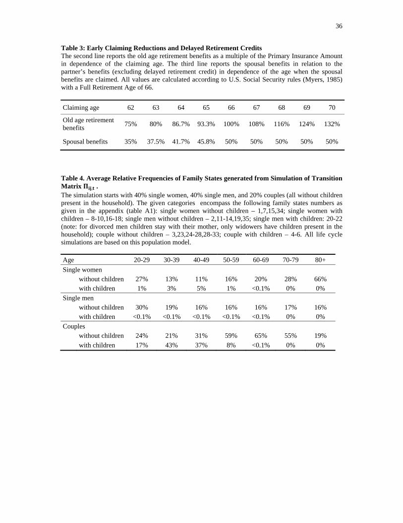
36  

 

Table 3: Early Claiming Reductions and Delayed Retirement Credits The second line reports the old age retirement benefits as a multiple of the Primary Insurance Amount in dependence of the claiming age. The third line reports the spousal benefits in relation to the partner’s benefits (excluding delayed retirement credit) in dependence of the age when the spousal benefits are claimed. All values are calculated according to U.S. Social Security rules (Myers, 1985) with a Full Retirement Age of 66.

Claiming age 62 63 64 65 66 67 68 69 70

Old age retirement benefits

75% 80% 86.7% 93.3% 100% 108% 116% 124% 132%

Spousal benefits 35% 37.5% 41.7% 45.8% 50% 50% 50% 50% 50%

Table 4. Average Relative Frequencies of Family States generated from Simulation of Transition Matrix , . The simulation starts with 40% single women, 40% single men, and 20% couples (all without children present in the household). The given categories encompass the following family states numbers as given in the appendix (table A1): single women without children – 1,7,15,34; single women with children – 8-10,16-18; single men without children – 2,11-14,19,35; single men with children: 20-22 (note: for divorced men children stay with their mother, only widowers have children present in the household); couple without children – 3,23,24-28,28-33; couple with children – 4-6. All life cycle simulations are based on this population model.

Age 20-29 30-39 40-49 50-59 60-69 70-79 80+

Single women without children 27% 13% 11% 16% 20% 28% 66%

with children 1% 3% 5% 1% <0.1% 0% 0%

Single men without children 30% 19% 16% 16% 16% 17% 16%

with children <0.1% <0.1% <0.1% <0.1% <0.1% 0% 0%

Couples

without children 24% 21% 31% 59% 65% 55% 19% with children 17% 43% 37% 8% <0.1% 0% 0%

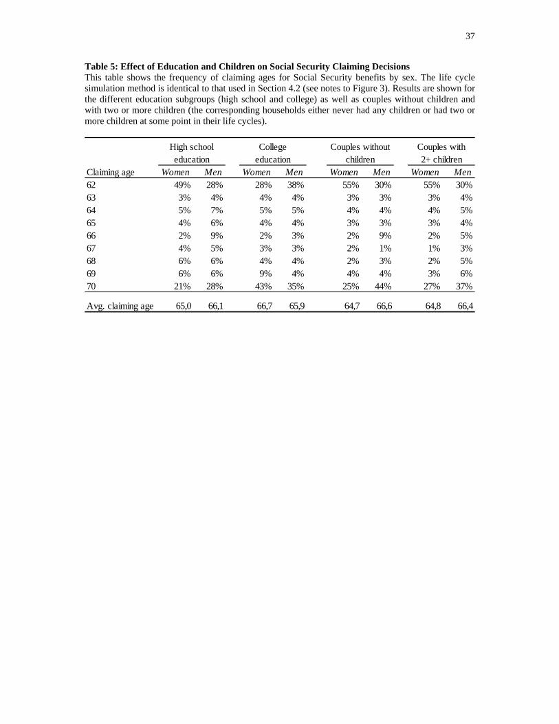
37  

 

Table 5: Effect of Education and Children on Social Security Claiming Decisions This table shows the frequency of claiming ages for Social Security benefits by sex. The life cycle simulation method is identical to that used in Section 4.2 (see notes to Figure 3). Results are shown for the different education subgroups (high school and college) as well as couples without children and with two or more children (the corresponding households either never had any children or had two or more children at some point in their life cycles).

Claiming age Women Men Women Men Women Men Women Men62 49% 28% 28% 38% 55% 30% 55% 30%63 3% 4% 4% 4% 3% 3% 3% 4%64 5% 7% 5% 5% 4% 4% 4% 5%65 4% 6% 4% 4% 3% 3% 3% 4%66 2% 9% 2% 3% 2% 9% 2% 5%67 4% 5% 3% 3% 2% 1% 1% 3%68 6% 6% 4% 4% 2% 3% 2% 5%69 6% 6% 9% 4% 4% 4% 3% 6%70 21% 28% 43% 35% 25% 44% 27% 37%

Avg. claiming age 65,0 66,1 66,7 65,9 64,7 66,6 64,8 66,4

High school education

College education

Couples without children

Couples with 2+ children

38  

 

Table 6: Effect of Education and Children on Stock Holdings as a Fraction of Financial Wealth

This table shows average stock holdings as a fraction of financial wealth for persons in different age groups. The life cycle simulation method is identical to that used in Section 4.2 (see notes to Figure 3). Results are shown for the different education subgroups (high school and college) as well as couples without children and with two or more children (the corresponding households either never had any children or had two or more children at some point in their life cycles).

Table 7: Normalized Life Insurance Values This table shows average life insurance face values by sex for different age groups. The values are given as multiples of the spouse’s income assuming full time work (40 hours per week). The life cycle simulation method is identical to that used in Section 4.2 (see notes to Figure 3). Results are shown for the different education subgroups (high school and college) as well as couples without children and with two or more children (the corresponding households either never had any children or had two or more children at some point in their life cycles).

 

AgeHigh school education

College education

Couples without children

Couples with 2+ children

25-34 51% 50% 60% 61%35-44 60% 61% 64% 59%45-54 54% 55% 58% 50%55-64 45% 52% 53% 44%65-74 46% 52% 53% 48%75-84 45% 48% 49% 47%

Age Women Men Women Men Women Men Women Men25-34 0.32 1.19 0.32 1.16 0.00 1.39 0.84 2.8635-44 0.81 1.92 0.63 1.75 0.15 2.23 1.70 3.3745-54 0.58 1.77 0.41 1.62 0.26 2.27 1.16 2.7555-64 0.04 1.35 0.02 1.25 0.02 1.84 0.07 2.0365-74 0.00 0.17 0.00 0.19 0.00 0.26 0.00 0.29

High school education

College education

Couples without children

Couples with 2+ children

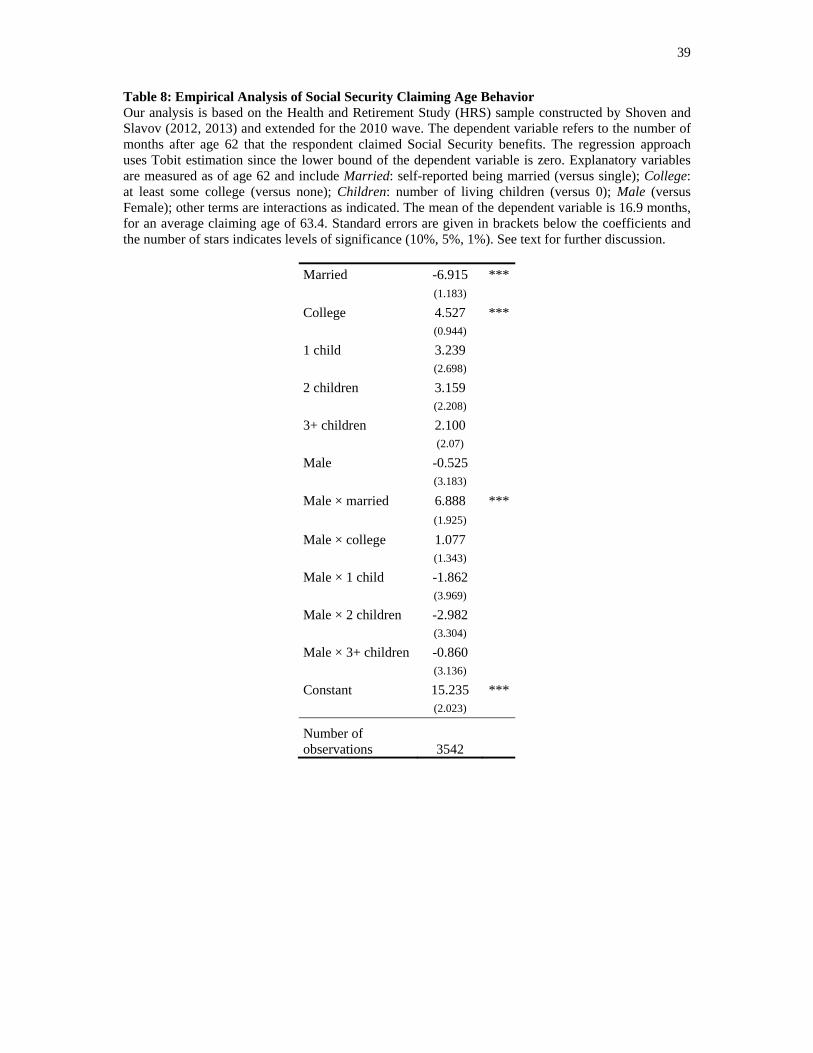
39  

 

Table 8: Empirical Analysis of Social Security Claiming Age Behavior Our analysis is based on the Health and Retirement Study (HRS) sample constructed by Shoven and Slavov (2012, 2013) and extended for the 2010 wave. The dependent variable refers to the number of months after age 62 that the respondent claimed Social Security benefits. The regression approach uses Tobit estimation since the lower bound of the dependent variable is zero. Explanatory variables are measured as of age 62 and include Married: self-reported being married (versus single); College: at least some college (versus none); Children: number of living children (versus 0); Male (versus Female); other terms are interactions as indicated. The mean of the dependent variable is 16.9 months, for an average claiming age of 63.4. Standard errors are given in brackets below the coefficients and the number of stars indicates levels of significance (10%, 5%, 1%). See text for further discussion.

Married -6.915 ***(1.183)

College 4.527 ***(0.944)

1 child 3.239 (2.698)

2 children 3.159 (2.208)

3+ children 2.100 (2.07)

Male -0.525 (3.183)

Male × married 6.888 ***(1.925)

Male × college 1.077 (1.343)

Male × 1 child -1.862 (3.969)

Male × 2 children -2.982 (3.304)

Male × 3+ children -0.860 (3.136)

Constant 15.235 *** (2.023)

Number of observations 3542

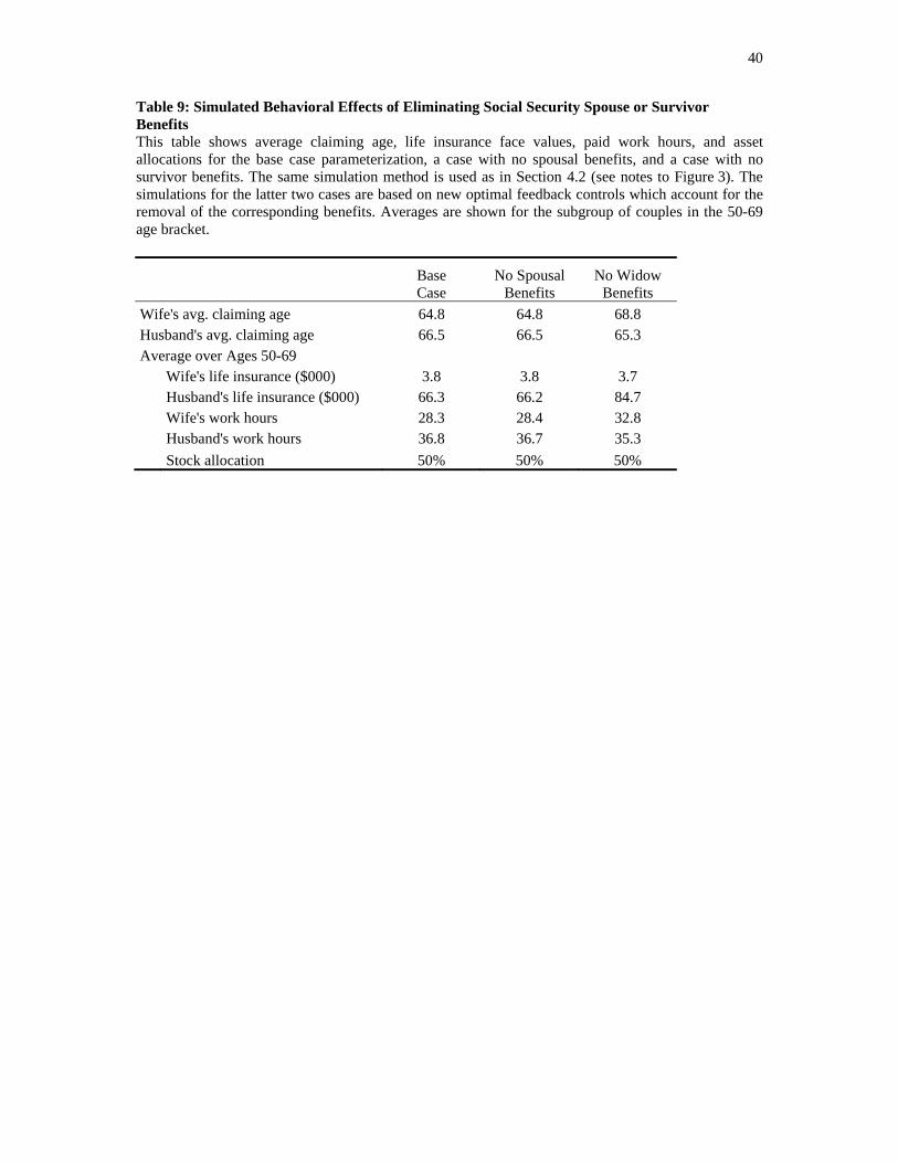
40  

 

Table 9: Simulated Behavioral Effects of Eliminating Social Security Spouse or Survivor Benefits This table shows average claiming age, life insurance face values, paid work hours, and asset allocations for the base case parameterization, a case with no spousal benefits, and a case with no survivor benefits. The same simulation method is used as in Section 4.2 (see notes to Figure 3). The simulations for the latter two cases are based on new optimal feedback controls which account for the removal of the corresponding benefits. Averages are shown for the subgroup of couples in the 50-69 age bracket.

Base Case

No Spousal Benefits

No Widow Benefits

Wife's avg. claiming age 64.8 64.8 68.8 Husband's avg. claiming age 66.5 66.5 65.3 Average over Ages 50-69

Wife's life insurance ($000) 3.8 3.8 3.7 Husband's life insurance ($000) 66.3 66.2 84.7 Wife's work hours 28.3 28.4 32.8 Husband's work hours 36.8 36.7 35.3

Stock allocation 50% 50% 50%

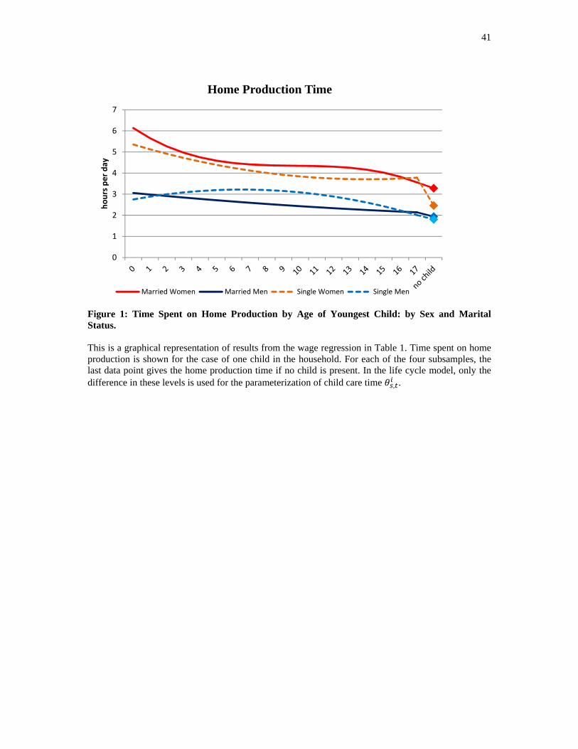
41  

 

Figure 1: Time Spent on Home Production by Age of Youngest Child: by Sex and Marital Status. This is a graphical representation of results from the wage regression in Table 1. Time spent on home production is shown for the case of one child in the household. For each of the four subsamples, the last data point gives the home production time if no child is present. In the life cycle model, only the difference in these levels is used for the parameterization of child care time , .     

0

1

2

3

4

5

6

7hours per day

age of youngest child

Home Production Time

Married Women Married Men Single Women Single Men

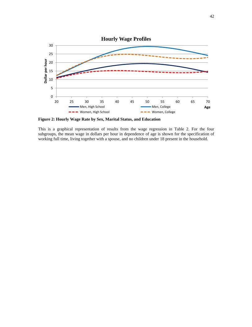
42  

 

 

Figure 2: Hourly Wage Rate by Sex, Marital Status, and Education This is a graphical representation of results from the wage regression in Table 2. For the four subgroups, the mean wage in dollars per hour in dependence of age is shown for the specification of working full time, living together with a spouse, and no children under 18 present in the household.    

0

5

10

15

20

25

30

20 25 30 35 40 45 50 55 60 65 70

Dollar per hour

Age

Hourly Wage Profiles

Men, High School Men, College

Women, High School Women, College

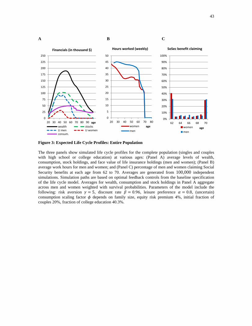
43  

 

A B C

Figure 3: Expected Life Cycle Profiles: Entire Population The three panels show simulated life cycle profiles for the complete population (singles and couples with high school or college education) at various ages: (Panel A) average levels of wealth, consumption, stock holdings, and face value of life insurance holdings (men and women); (Panel B) average work hours for men and women; and (Panel C) percentage of men and women claiming Social Security benefits at each age from 62 to 70. Averages are generated from 100,000 independent simulations. Simulation paths are based on optimal feedback controls from the baseline specification of the life cycle model. Averages for wealth, consumption and stock holdings in Panel A aggregate across men and women weighted with survival probabilities. Parameters of the model include the following: risk aversion 5, discount rate 0.96, leisure preference 0.8, (uncertain) consumption scaling factor depends on family size, equity risk premium 4%, initial fraction of couples 20%, fraction of college education 40.3%.

0

25

50

75

100

125

150

175

200

225

250

20 30 40 50 60 70 80 90 100age

Financials (in thousand $)

wealth stocksLI men LI womenconsum.

0

5

10

15

20

25

30

35

40

45

50

20 30 40 50 60 70 80

age

Hours worked (weekly)

women

men

0%

10%

20%

30%

40%

50%

60%

70%

80%

90%

100%

62 64 66 68 70

age

SoSec benefit claiming

women

men

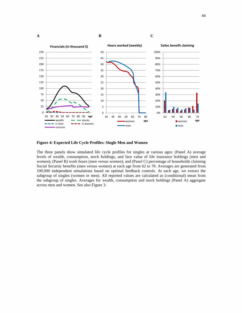
44  

 

A B C

Figure 4: Expected Life Cycle Profiles: Single Men and Women The three panels show simulated life cycle profiles for singles at various ages: (Panel A) average levels of wealth, consumption, stock holdings, and face value of life insurance holdings (men and women); (Panel B) work hours (men versus women); and (Panel C) percentage of households claiming Social Security benefits (men versus women) at each age from 62 to 70. Averages are generated from 100,000 independent simulations based on optimal feedback controls. At each age, we extract the subgroup of singles (women or men). All reported values are calculated as (conditional) mean from the subgroup of singles. Averages for wealth, consumption and stock holdings (Panel A) aggregate across men and women. See also Figure 3.

0

25

50

75

100

125

150

175

200

225

250

20 30 40 50 60 70 80 90 100age

Financials (in thousand $)

wealth stocksLI men LI womenconsum.

0

5

10

15

20

25

30

35

40

45

50

20 30 40 50 60 70 80

age

Hours worked (weekly)

women

men

0%

10%

20%

30%

40%

50%

60%

70%

80%

90%

100%

62 64 66 68 70age

SoSec benefit claiming

women

men

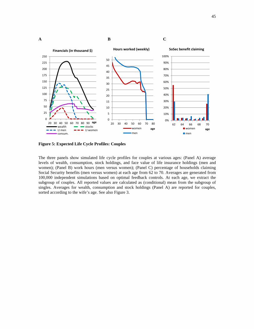
45  

 

A B C

Figure 5: Expected Life Cycle Profiles: Couples

The three panels show simulated life cycle profiles for couples at various ages: (Panel A) average levels of wealth, consumption, stock holdings, and face value of life insurance holdings (men and women); (Panel B) work hours (men versus women); (Panel C) percentage of households claiming Social Security benefits (men versus women) at each age from 62 to 70. Averages are generated from 100,000 independent simulations based on optimal feedback controls. At each age, we extract the subgroup of couples. All reported values are calculated as (conditional) mean from the subgroup of singles. Averages for wealth, consumption and stock holdings (Panel A) are reported for couples, sorted according to the wife’s age. See also Figure 3.

0

25

50

75

100

125

150

175

200

225

250

20 30 40 50 60 70 80 90 100age 

Financials (in thousand $)

wealth stocksLI men LI womenconsum.

0

5

10

15

20

25

30

35

40

45

50

20 30 40 50 60 70 80

age

Hours worked (weekly)

women

men

0%

10%

20%

30%

40%

50%

60%

70%

80%

90%

100%

62 64 66 68 70

age

SoSec benefit claiming

women

men

46  

 

Appendix A: Family States Modeled in Our Study This table shows the different family states in our model. The third column lists the states to which stochastic transitions are possible. The fourth column lists states to which transitions are possible by one or both spouses claiming retirement benefits. State number

Description Possible stochastic transitions Possible claiming transitions

1 single woman (never married) 1, 3 34

2 single man (never married) 2, 3 35

3 couple without children 3-4, 7-8, 11-12, 15-16, 19-20 23,24-28, 29-33

4 couple with 1 child 3-5, 7-9, 11-13, 15-17, 19-21 -

5 couple with 2 children 4-6, 8-10, 12-14, 16-18, 20-22 -

6 couple with 3 or more children 5-6, 9-10, 13-14, 17-18, 21-22 -

7 divorced woman without children 3,7 34

8 divorced woman with 1 child 3-4, 7-8 -

9 divorced woman with 2 children 4-5, 8-9 -

10 divorced woman with 3 or more children 5-6, 9-10 -

11 divorced man without children 3, 11 35

12 divorced man with 1 child 3-4, 11-12 -

13 divorced man with 2 children 4-5, 12-13 -

14 divorced man with 3 or more children 5-6, 13-14 -

15 widow without children 3, 15 34

16 widow with 1 child 3-4, 15-16 -

17 widow with 2 children 4-5, 16-17 -

18 widow with 3 or more children 5-6, 17-18 -

19 widower without children 3, 19 35

20 widower with 1 child 3-4, 19-20 -

21 widower with 2 children 4-5, 20-21 -

22 widower with 3 or more children 5-6, 21-22 -

23 couple with retired wife 19, 23, 34 29-33

24 couple with retired husband (claimed at 66 or before) 15, 24, 35 29

25 couple with retired husband (claimed at 67) 15, 25, 35 30

26 couple with retired husband (claimed at 68) 15, 26, 35 31

27 couple with retired husband (claimed at 69) 15, 27, 35 32

28 couple with retired husband (claimed at 70) 15, 28, 35 33

29 retired couple (husband claimed at 66 or before) 29, 34, 35 -

30 retired couple (husband claimed at 67) 30, 34, 35 -

31 retired couple (husband claimed at 68) 31, 34, 35 -

32 retired couple (husband claimed at 69) 32, 34, 35 -

33 retired couple (husband claimed at 70) 33, 34, 35 -

34 single retired woman 34 -

35 single retired man 35 -

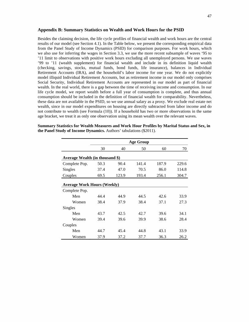
47  

 

Appendix B: Summary Statistics on Wealth and Work Hours for the PSID

Besides the claiming decision, the life cycle profiles of financial wealth and work hours are the central results of our model (see Section 4.1). In the Table below, we present the corresponding empirical data from the Panel Study of Income Dynamics (PSID) for comparison purposes. For work hours, which we also use for inferring the wages in Section 3.3, we use the more recent subsample of waves ‘95 to ’11 limit to observations with positive work hours excluding all unemployed persons. We use waves ’99 to ’11 (wealth supplement) for financial wealth and include in its definition liquid wealth (checking, savings, stocks, mutual funds, bond funds, life insurance), balances in Individual Retirement Accounts (IRA), and the household’s labor income for one year. We do not explicitly model illiquid Individual Retirement Accounts, but as retirement income in our model only comprises Social Security, Individual Retirement Accounts are represented in our model as part of financial wealth. In the real world, there is a gap between the time of receiving income and consumption. In our life cycle model, we report wealth before a full year of consumption is complete, and thus annual consumption should be included in the definition of financial wealth for comparability. Nevertheless, these data are not available in the PSID, so we use annual salary as a proxy. We exclude real estate net wealth, since in our model expenditures on housing are directly subtracted from labor income and do not contribute to wealth (see Formula (10)). If a household has two or more observations in the same age bracket, we treat it as only one observation using its mean wealth over the relevant waves. Summary Statistics for Wealth Measures and Work Hour Profiles by Marital Status and Sex, in the Panel Study of Income Dynamics. Authors’ tabulations ($2011).

Age Group

30 40 50 60 70

Average Wealth (in thousand $)

Complete Pop. 50.3 90.4 141.4 187.9 229.6 Singles 37.4 47.0 70.5 86.0 114.8

Couples 69.5 123.9 193.4 256.1 304.7

Average Work Hours (Weekly)

Complete Pop. Men 44.4 44.9 44.5 42.6 33.9 Women 38.4 37.9 38.4 37.1 27.3

Singles Men 43.7 42.5 42.7 39.6 34.1 Women 39.4 39.6 39.9 38.6 28.4

Couples Men 44.7 45.4 44.8 43.1 33.9

Women 37.9 37.2 37.7 36.3 26.2

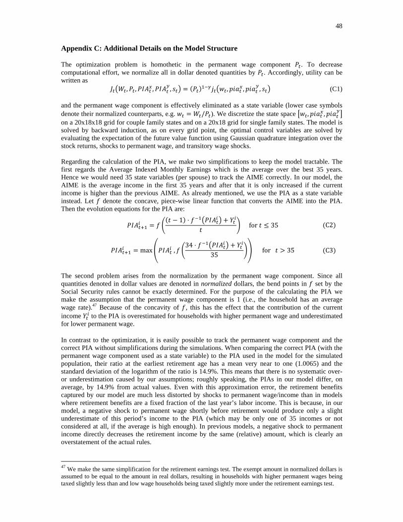
48  

 

Appendix C: Additional Details on the Model Structure The optimization problem is homothetic in the permanent wage component . To decrease computational effort, we normalize all in dollar denoted quantities by . Accordingly, utility can be written as

, , , , , , , (C1) and the permanent wage component is effectively eliminated as a state variable (lower case symbols denote their normalized counterparts, e.g. / ). We discretize the state space , , on a 20x18x18 grid for couple family states and on a 20x18 grid for single family states. The model is solved by backward induction, as on every grid point, the optimal control variables are solved by evaluating the expectation of the future value function using Gaussian quadrature integration over the stock returns, shocks to permanent wage, and transitory wage shocks. Regarding the calculation of the PIA, we make two simplifications to keep the model tractable. The first regards the Average Indexed Monthly Earnings which is the average over the best 35 years. Hence we would need 35 state variables (per spouse) to track the AIME correctly. In our model, the AIME is the average income in the first 35 years and after that it is only increased if the current income is higher than the previous AIME. As already mentioned, we use the PIA as a state variable instead. Let denote the concave, piece-wise linear function that converts the AIME into the PIA. Then the evolution equations for the PIA are: 1 ⋅

for 35  C2

max ,

34 ⋅35

for 35  C3

 The second problem arises from the normalization by the permanent wage component. Since all quantities denoted in dollar values are denoted in normalized dollars, the bend points in set by the Social Security rules cannot be exactly determined. For the purpose of the calculating the PIA we make the assumption that the permanent wage component is 1 (i.e., the household has an average wage rate).47 Because of the concavity of , this has the effect that the contribution of the current income to the PIA is overestimated for households with higher permanent wage and underestimated for lower permanent wage.  In contrast to the optimization, it is easily possible to track the permanent wage component and the correct PIA without simplifications during the simulations. When comparing the correct PIA (with the permanent wage component used as a state variable) to the PIA used in the model for the simulated population, their ratio at the earliest retirement age has a mean very near to one (1.0065) and the standard deviation of the logarithm of the ratio is 14.9%. This means that there is no systematic over- or underestimation caused by our assumptions; roughly speaking, the PIAs in our model differ, on average, by 14.9% from actual values. Even with this approximation error, the retirement benefits captured by our model are much less distorted by shocks to permanent wage/income than in models where retirement benefits are a fixed fraction of the last year’s labor income. This is because, in our model, a negative shock to permanent wage shortly before retirement would produce only a slight underestimate of this period’s income to the PIA (which may be only one of 35 incomes or not considered at all, if the average is high enough). In previous models, a negative shock to permanent income directly decreases the retirement income by the same (relative) amount, which is clearly an overstatement of the actual rules.

                                                            47 We make the same simplification for the retirement earnings test. The exempt amount in normalized dollars is assumed to be equal to the amount in real dollars, resulting in households with higher permanent wages being taxed slightly less than and low wage households being taxed slightly more under the retirement earnings test.