how embedding of social ties in space impacts human...
TRANSCRIPT

HOW EMBEDDING OF SOCIAL TIES IN SPACEIMPACTS HUMAN BEHAVIOR
By
Herbert O. Holzbauer
A Thesis Submitted to the Graduate
Faculty of Rensselaer Polytechnic Institute
in Partial Fulfillment of the
Requirements for the Degree of
DOCTOR OF PHILOSOPHY
Major Subject: COMPUTER SCIENCE
Approved by theExamining Committee:
Boleslaw K. Szymanski, Thesis Adviser
Barbara M. Cutler, Member
Malik Magdon-Ismail, Member
Gyorgy Korniss, Member
Rensselaer Polytechnic InstituteTroy, New York
November 2016(For Graduation December 2016)

c© Copyright 2016
by
Herbert O. Holzbauer
All Rights Reserved
ii

CONTENTS
LIST OF TABLES . . . . . . . . . . . . . . . . . . . . . . . . . . . . . . . . . v
LIST OF FIGURES . . . . . . . . . . . . . . . . . . . . . . . . . . . . . . . . vi
ACKNOWLEDGMENT . . . . . . . . . . . . . . . . . . . . . . . . . . . . . . viii
ABSTRACT . . . . . . . . . . . . . . . . . . . . . . . . . . . . . . . . . . . . ix
1. Introduction . . . . . . . . . . . . . . . . . . . . . . . . . . . . . . . . . . . 1
2. Related Work . . . . . . . . . . . . . . . . . . . . . . . . . . . . . . . . . . 3
2.1 Participatory Sensing . . . . . . . . . . . . . . . . . . . . . . . . . . . 3
2.1.1 Incentives and Sensing . . . . . . . . . . . . . . . . . . . . . . 4
2.1.2 Privacy Oriented Approaches . . . . . . . . . . . . . . . . . . 13
2.1.3 Participatory Sensing Systems . . . . . . . . . . . . . . . . . . 25
2.2 Social Ties . . . . . . . . . . . . . . . . . . . . . . . . . . . . . . . . . 27
2.3 Milgram Experiments . . . . . . . . . . . . . . . . . . . . . . . . . . . 29
3. Incentivizing Participatory Sensing via Auction Mechanisms . . . . . . . . 32
3.1 Problem Definition . . . . . . . . . . . . . . . . . . . . . . . . . . . . 33
3.2 Issues in Participatory Sensing . . . . . . . . . . . . . . . . . . . . . . 33
3.2.1 Data . . . . . . . . . . . . . . . . . . . . . . . . . . . . . . . . 33
3.2.2 Coordination . . . . . . . . . . . . . . . . . . . . . . . . . . . 34
3.2.3 Privacy and Security . . . . . . . . . . . . . . . . . . . . . . . 35
3.2.4 Human Concerns . . . . . . . . . . . . . . . . . . . . . . . . . 37
3.2.5 Participants . . . . . . . . . . . . . . . . . . . . . . . . . . . . 38
3.3 Applying Market Mechanisms . . . . . . . . . . . . . . . . . . . . . . 38
3.3.1 Notes on CarTel . . . . . . . . . . . . . . . . . . . . . . . . . . 46
3.3.2 Notes on SORA . . . . . . . . . . . . . . . . . . . . . . . . . . 47
3.4 Privacy, Power, and Participation-aware Auction Mechanism . . . . . 48
3.5 Summary . . . . . . . . . . . . . . . . . . . . . . . . . . . . . . . . . 53
4. Using Social Interactions as Predictors of Success . . . . . . . . . . . . . . 57
4.1 Motivation and Background . . . . . . . . . . . . . . . . . . . . . . . 57
4.2 Data . . . . . . . . . . . . . . . . . . . . . . . . . . . . . . . . . . . . 59
iii

4.3 Methods . . . . . . . . . . . . . . . . . . . . . . . . . . . . . . . . . . 61
4.3.1 Idea Flow . . . . . . . . . . . . . . . . . . . . . . . . . . . . . 61
4.3.2 Social Diversity . . . . . . . . . . . . . . . . . . . . . . . . . . 62
4.3.3 Estimation of the Exponential Distribution . . . . . . . . . . . 63
4.3.3.1 Method #1: Approximation . . . . . . . . . . . . . . 65
4.3.3.2 Method #2: Zeroing Parameters . . . . . . . . . . . 67
4.3.3.3 Method #3: Mixed Solutions . . . . . . . . . . . . . 68
4.3.3.4 Iteration on Parameters . . . . . . . . . . . . . . . . 70
4.3.4 Estimation of the Gaussian Distribution . . . . . . . . . . . . 73
4.3.4.1 Linear Approximation . . . . . . . . . . . . . . . . . 74
4.3.4.2 Iteration on Parameters . . . . . . . . . . . . . . . . 80
4.3.5 Short and Long Tie Counting . . . . . . . . . . . . . . . . . . 83
4.4 Results . . . . . . . . . . . . . . . . . . . . . . . . . . . . . . . . . . . 84
4.5 Discussion . . . . . . . . . . . . . . . . . . . . . . . . . . . . . . . . . 88
4.6 Summary . . . . . . . . . . . . . . . . . . . . . . . . . . . . . . . . . 90
5. Influence of Knowledge of Friend of Friends on Social Search . . . . . . . . 91
5.1 Background . . . . . . . . . . . . . . . . . . . . . . . . . . . . . . . . 91
5.2 Methods . . . . . . . . . . . . . . . . . . . . . . . . . . . . . . . . . . 92
5.3 Results . . . . . . . . . . . . . . . . . . . . . . . . . . . . . . . . . . . 98
5.4 Discussion . . . . . . . . . . . . . . . . . . . . . . . . . . . . . . . . . 104
5.5 Summary . . . . . . . . . . . . . . . . . . . . . . . . . . . . . . . . . 120
6. Conclusion . . . . . . . . . . . . . . . . . . . . . . . . . . . . . . . . . . . . 126
6.1 Contributions . . . . . . . . . . . . . . . . . . . . . . . . . . . . . . . 126
6.2 Limitations . . . . . . . . . . . . . . . . . . . . . . . . . . . . . . . . 127
6.3 Future Work . . . . . . . . . . . . . . . . . . . . . . . . . . . . . . . . 129
REFERENCES . . . . . . . . . . . . . . . . . . . . . . . . . . . . . . . . . . . 130
iv

LIST OF TABLES
4.1 Summary of Geographic Ties and Strength-Based Ties . . . . . . . . . . 61
4.2 Correlations Between Indicators and Economic Metrics . . . . . . . . . 84
4.3 Exponential MLE of Indicators Fit to Economic Metrics . . . . . . . . . 86
4.4 Gaussian MLE of Indicators Fit to Economic Metrics . . . . . . . . . . 86
4.5 MLE Differences for Confidence Levels Using LRT (χ2) . . . . . . . . . 87
4.6 Mapping of ∆AIC and χ2 Values to Qualitative Categories . . . . . . . 87
5.1 Friendship Density by Distance Range, US-Only . . . . . . . . . . . . . 96
5.2 Social Search Results on Global . . . . . . . . . . . . . . . . . . . . . . 99
5.3 Social Search Results on US-Only . . . . . . . . . . . . . . . . . . . . . 100
5.4 Social Search Results on Filtered . . . . . . . . . . . . . . . . . . . . . . 101
5.5 Additional Low-κ Social Search Results For US-Only . . . . . . . . . . 107
5.6 Adverse Effects of Increasing κ on US-Only . . . . . . . . . . . . . . . . 108
5.7 Friendship Density by Distance Range, Filtered . . . . . . . . . . . . . . 118
5.8 US-Only Community Density by Distance Range . . . . . . . . . . . . . 119
5.9 Filtered Community Density by Distance Range . . . . . . . . . . . . . 120
5.10 Metropolitan Representation in Gowalla vs United States . . . . . . . . 121
v

LIST OF FIGURES
3.1 P3AM: Average Contributor Battery Level, Taxi Mobility . . . . . . . . 51
3.2 P3AM: Average Contributor Battery Level, Random Mobility . . . . . . 52
3.3 P3AM Average Price per Measurement, Taxi Mobility . . . . . . . . . . 54
3.4 P3AM Average Price per Measurement Zoomed In, Taxi Mobility . . . 55
3.5 P3AM: Average Price per Measurement, Random Mobility . . . . . . . 56
4.1 US Metros in Gowalla, Grid Based . . . . . . . . . . . . . . . . . . . . . 60
4.2 Gaussian Distribution Models Grouped by Equivalence Class . . . . . . 88
5.1 Successful DP Chain Lengths in US-Only . . . . . . . . . . . . . . . . . 102
5.2 Successful DP Chain Lengths in Filtered . . . . . . . . . . . . . . . . . 103
5.3 Successful DP Chain Lengths in Global . . . . . . . . . . . . . . . . . . 104
5.4 Successful CD Chain Lengths in US-Only . . . . . . . . . . . . . . . . . 105
5.5 Successful CD Chain Lengths in Global . . . . . . . . . . . . . . . . . . 106
5.6 Path Consistency in US-Only . . . . . . . . . . . . . . . . . . . . . . . . 109
5.7 Gowalla Degree Distribution, Global . . . . . . . . . . . . . . . . . . . . 110
5.8 Gowalla Degree Distribution, US-Only . . . . . . . . . . . . . . . . . . . 110
5.9 Gowalla Degree Distribution, Filtered . . . . . . . . . . . . . . . . . . . 111
5.10 Gowalla Global CCDF . . . . . . . . . . . . . . . . . . . . . . . . . . . 111
5.11 Gowalla US-Only CCDF . . . . . . . . . . . . . . . . . . . . . . . . . . 112
5.12 Gowalla Filtered CCDF . . . . . . . . . . . . . . . . . . . . . . . . . . . 113
5.13 Gowalla Friends of Friends Distribution, US-Only . . . . . . . . . . . . 113
5.14 Gowalla Friends of Friends Distribution, Filtered . . . . . . . . . . . . . 114
5.15 Community Sizes, US-Only . . . . . . . . . . . . . . . . . . . . . . . . . 114
5.16 Community Sizes, Filtered . . . . . . . . . . . . . . . . . . . . . . . . . 115
5.17 Metropolitan Areas in Gowalla, US-Only . . . . . . . . . . . . . . . . . 115
vi

5.18 Trial Start Locations in Gowalla, US-Only . . . . . . . . . . . . . . . . 116
5.19 Trial Target Locations in Gowalla, US-Only . . . . . . . . . . . . . . . . 116
5.20 Random Start Locations in Gowalla, US-Only . . . . . . . . . . . . . . 117
5.21 Random Target Locations in Gowalla, US-Only . . . . . . . . . . . . . . 117
5.22 Community Membership by Friends Distribution, US-Only . . . . . . . 122
5.23 Community Membership by Friends of Friends Distribution, US-Only . 122
5.24 Friends Within Community Distribution, US-Only . . . . . . . . . . . . 123
5.25 Friend of Friends Within Community Distribution, US-Only . . . . . . 123
5.26 Community Membership by Friends Distribution, Filtered . . . . . . . . 124
5.27 Community Membership by Friends of Friends Distribution, Filtered . . 124
5.28 Friends Within Community Distribution, Filtered . . . . . . . . . . . . 125
5.29 Friend of Friends Within Community Distribution, Filtered . . . . . . . 125
vii

ACKNOWLEDGMENT
I’m very grateful to Boleslaw Szymanski for serving the integral role of being my
adviser during my Ph. D process and for the numerous opportunities he’s given
me, the support he’s given me in all stages of research from problem design to
approaches to interpretation, as well as the chances to develop my own research
abilities. I’d like to thank Alex “Sandy” Pentland for continuing to provide his
amazing insights regarding my work and providing invaluable perspective into the
scientific publication process throughout my graduate student career. I’d also like
to thank Brandon Thorne and Miao Qi for their excellent software development
support, which was key to bringing the last portion of the dissertation to fruition.
I’d also like to thank those that gave me additional support, guidance, and
helped make these last few years a particularly pleasant experience: Barbara Cut-
ler, Christopher Stuetzle, Joshua Nasman, Elsa Gonsiorowski, Justin LaPre, Pam
Paslow, Jeanne Rice, and Christopher Heffron. Without all of you, I can’t imagine
what the last few years would have been like.
Research was partially sponsored by the Army Research Laboratory and was
accomplished under Cooperative Agreement Number W911NF-09-2-0053 (the ARL
Network Science CTA) and by the Office of Naval Research Contracts N00014-09-1-
0607 and N00014-15-1-2640. The content of this document do not necessarily reflect
the position or policy of the U.S. Government, ARL or ONR, no official endorsement
should be inferred or implied.
viii

ABSTRACT
A social network is a collection of users and relationships between them, typically
viewed as a graph. The most common type of relationship is a friendship, such as
seen in popular social networking platforms like Facebook. However, these networks
exist in a variety of contexts both online and offline. Regardless of the medium or
context, they allow us to quantify relationships between individual humans. These
social networks, and the underlying communities they describe, contribute to our
understanding of human behavior. Specifically we consider the impact of these ties
when they are embedded in space.
We first demonstrate this indirectly in incentivized participatory sensing (where
humans voluntarily perform sensing tasks in exchange for rewards) by leveraging hu-
man mobility, intelligence, and technology to select and collect evidence of events
and phenomena occurring in the real world. We utilize a set of traces derived from
actual human mobility and compare this to previously published work in which
we had a similar system but employed random synthetic mobility. Based on the
differences, we propose that human mobility is a critical part of understanding op-
portunistic networks such as the participatory sensing problem we studied.
We then directly use a location-based service with a social network, Gowalla,
towards two goals. The first is to analyze artificial social searches inspired by Mil-
gram’s small world experiments (delivering a package to a target using real ac-
quaintances). By creating protocols which a rational agent could use for making
forwarding decisions, we are able to explore the effect of several network features,
and of partial knowledge of friends-of-friends on the social search.
We also use Gowalla to predict economic performance in the form of United
States (US) Gross Domestic Product (GDP) using both the geographic location
and social links of Gowalla users. We find that long ties (those that cross state
boundaries) are an invaluable tool in estimation of GDP. We also discuss use of the
predictors we develop in two other economic contexts, but ultimately find that these
metrics are ill-suited for our approach and we explore why.
ix

CHAPTER 1
Introduction
Social networks are networks (collections of nodes that are connected by edges),
where the nodes are human beings and the edges are some sort of social relationship.
Most commonly the relationship is a friendship, however it is not the only possible
reason humans can be connected. For example, a social network may be composed
of individuals who are related because of services they exchange with others in
the network. Within social networks, there is a lot of potential for research due
to the rich and large body of data available and the underlying human behavior
that is expressed as the social network and events in the network. Popular modern
examples of social networks are LiveJournal (‘journal’ blogging), Tumblr (image
blogging), Facebook, and Google+. Many other such networks exist, spanning a
broad array of applications and each having their own features. In many cases, we
can infer additional networks from interactions or other analysis like community
detection.
Our claim is that these social networks allow us insight into phenomena in-
fluenced by complex human behaviors that are difficult to understand by observing
individuals independently. We substantiate this through three different research
topics after first exploring related work in Chapter 2:
• In Chapter 3 we consider a participatory sensing scenario in which humans
volunteer their devices for a distributed sensing task. Due to the dependence
of the system on geographic positioning of humans over time, the impact of hu-
man mobility on such a system becomes a question. We explore whether sim-
ply addressing human concerns can remove this dependency, and the impact
of human mobility based on taxi traces taken in San Francisco. Since profes-
sional and social obligations influence who we interact with and subsequently
where we go, these traces offer a way to see the relevant (i.e. spatiotemporal)
impact of human relationships on our application without having to know the
underlying social network features.
1

2
• In Chapter 4 we examine a location-based social network, Gowalla, and use
various properties as indicators for real-world economic metrics from 2012.
• In Chapter 5 we look at an artificial social search task inspired by the well-
studied “small world” effect to explore the impact that knowledge of friends-
of-friends (FoFs) has on the efficiency and success of the task. More broadly,
we consider how the amount and specific kinds of knowledge one has about
their friends and FoFs impacts that individual’s reach within the network.
• Finally, we conclude with a summary of contributions, limitations, possible
ideas for future work, and closing remarks in Chapter 6.

CHAPTER 2
Related Work
The related work involving our participatory sensing research in Chapter 3 is quite
lengthy since our task is a synthesis of several different ideas in existing research.
We believe that presenting the existing literature in a survey format is more bene-
ficial to the reader, since it allows us to discuss our design approach in Chapter 3
without confusing our decisions with existing work done by other researchers. To
help with organization, it is further broken down into subsections on incentives
(Section 2.1.1), privacy (Section 2.1.2), and existing participatory sensing imple-
mentations (Section 2.1.3). We devote the rest of the chapter to early literature on
weak ties (Section 2.2) and small world experiments (Section 2.3), with the majority
of references to existing work applicable to Chapters 4–5 being introduced at the
beginning of the relevant chapters.
2.1 Participatory Sensing
In order to monitor the environment, sensors have been used in a variety of
situations ranging from static deployments such as personal weather monitoring to
mobile swarms of nodes designed to locate and track phenomena [1–4].
By using the mobility of living organisms, such as animals in ZebraNet [5],
device energy does not have to be used for movement. Carriers will always go to areas
of their interests, whether or not the application is suited to their lives. In ZebraNet,
where the goal is to track a zebra population, the application is inherent to mobility
of the carriers, which are the zebras themselves. Vehicles often have on-board GPS
and navigation tools, and third party sensing devices such as insurance companies
measuring acceleration habits through additional hardware are also implemented
Portions of this chapter previously appeared as: B. O. Holzbauer, B. K. Szymanski, andE. Bulut, “Incentivizing participatory sensing via auction mechanisms,” in Opportunistic MobileSocial Networks. Boca Raton, FL: CRC Press, 2014, ch. 12, pp. 339–736.Portions of this chapter previously appeared as: B. O. Holzbauer, B. K. Szymanski, T. Nguyen, andA. Pentland, “Social ties as predictors of economic development,” in Int. Conf. School NetworkSci., Wroc law, Poland, 2016, pp. 178–185.
3

4
in the real world. Portable personal devices such as smartphones, media players,
tablets, laptops, and even fitness trackers offer a wealth of data tethered to humans
and centered around human interests. Beyond simple mobility these allow a rich
variety of data which can be applied towards many tasks, such as measuring road
traffic congestion (one deployment being Waze), creating paths for cycling [2], and
large-scale modeling of human mobility. Additional examples are present throughout
the discussion of participatory system design in Chapter 3.
2.1.1 Incentives and Sensing
There are many challenges in participatory sensing design, many of which cen-
ter around human concerns. These are an integral part of the topic, since humans
willfully participating are the reason that such systems can be considered partici-
patory. We go into more depth in Section 3.2, however for the moment we focus on
the need to incentivize users both to ensure their continued participation, and to
offset perceived costs about loss of privacy or other resources. As such, we start by
looking at how to sustain participation over time, since long-term participation even
with incentives can result in significant loss of participants [6]. In short, recruiting
participants is a competition maintenance strategy, and without competition either
incentive budget is compromised by participants having too much control over pric-
ing, or user resources are overconsumed due to the system selecting from a pool of
sources that is too limited to sustain balanced source selection.
We now briefly look at a paper by Lee and Hoh [7] which described an auc-
tion mechanism, RADP-VPC, with more details discussed in Section 3.3. Within
the paper the authors reason that since participants can drop out, recruiting for-
mer participants is a useful technique. If a participant dropped out, it means that
the market conditions were not yielding incentive that matched their expectations,
either because they felt they won too infrequently, or because the incentive they
were receiving given the current competition was below their perceived utility of
participating. However, since the environment and prices are dynamic, it is possible
that at a future point in time the distribution of bids will have changed such that
a participant could rejoin and start winning. To facilitate recruiting former partici-

5
pants, any participant who is no longer participating is shown the highest price that
won in the most recent round. If a participant sees that its true valuation is less
than or equal to this revealed price, it should rejoin. The authors assume that only
participants who have dropped out will receive this information. Suggested methods
of delivery are e-mail and SMS. A participant who has dropped out then needs to
decide whether or not rejoining will be beneficial. To do this, the participant needs
to calculate the expected ROI of rejoining. The authors use the following definition:
“Let participant i at round r have participated in pri rounds prior to r, with
true valuation ti, tolerance to loss βi, and receive revealed price ϕr. Then the
expected ROI, ESr+1i is”:
ESri =eri + ϕr + βi
(pri + 1) · ti + βi(2.1)
To evaluate the performance of RADP-VPC, the authors compare it to the
Random Selection based Fixed Price (RSFP) mechanism, which randomly chooses
participants until quality of service is met for the round, and pays them each a
fixed price. Conceptually, the authors believe that RADP is better than RSFP from
the service provider’s view. This is because participants make the decisions about
their prices based on their knowledge about current valuations, as opposed to RSFP
where the mechanism is responsible for selecting a value that will satisfy the users’
price expectations. To study the behavior of the mechanisms, strategies must be
defined for the users (otherwise known as agents) who participate. The authors
assume risk-neutral agents which react to winning or losing by modifying their bids.
The authors formulate the utility Ui for participant i as follows:
“Let Ui be the utility for participant i, bidding bri in round r with credit for
winning ci(bri ), true valuation ti, and probability gi(b
ri ) of winning by bidding bri .
Then”
Ui(bri ) = (ci(b
ri )− ti) · gi(bri ) (2.2)
Furthermore, the attribute of “risk-neutral” is important. When considering
agent behavior, a designer must take into account how they view risk. Using the
standard auction terminology the authors distinguish the three risk attitudes and

6
their corresponding objectives, namely preference, neutrality, and aversion.
The descriptions of the experiments conducted can be found in the original
paper. The results show that for a variety of distributions of ti RADP-VPC results
in lower total cost than RSFP. This is because in RADP-VPC, lower bid prices
are favored. Because VPC prevents price explosion from happening, RADP-VPC
results in a more efficient use of budget, which is reflected in the total cost being
lower. The authors do not discuss how to tune the virtual credit parameter, α,
but observe that while initially increasing it results in a higher number of active
participants, after a certain α the number of participants starts to decrease. This
suggests that there is an optimal value for α. If the parameter is set too low, then
the addition of recruitment can still result in lower total cost, since the dynamic
nature of market is advertised to participants which can then rejoin based on their
ESri .
The next paper we examine describes a system designed to study recycling
practices at a university [6]. The measurements consisted of photographs of locations
where trash and recycling were deposited (such as “waste bins”) and optional tags
that participants could input prior to submitting the photographs. This system is
of particular interest to our design both because it is an example of asynchronous
participatory sensing, and because it explores the effect of different incentive schemes
applied to the task. While incentive does not necessarily involve application of the
concepts introduced earlier regarding markets, the COMPETE mechanism which is
described in the following discussion creates incentive-driven competition with the
goal of promoting participation.
The authors define participatory sensing based on three requirements:
1. “Users are involved in decisions about what will be collected.” This is the same
belief as expressed while discussing participatory privacy [8] at the beginning
of Section 2.1.2, which has authors in common with this paper.
2. “Users contribute data collected during daily routines.” The mention of daily
routines is important since it suggests that participatory sensing systems are
tied to the patterns in human behavior.

7
3. “Users are connected to the context/purpose of the tasks they perform.”
Five incentive schemes were considered, four of which were micro-payment
schemes. Micro-payments are incentive rewarded on a smaller, more frequent level.
The incentive use discussed previously throughout [6] has all been micro-payments
since incentive is awarded based on single actions or measurements. To make a fair
comparison between the five schemes, the maximum payout from each scheme was
the same, namely the MACRO amount. The authors define the following schemes:
• MACRO: One large payment for joining the experiment
• HIGHµ: 50 cents/valid measurement
• MEDIUMµ: 20 cents/valid measurement
• LOWµ: 5 cents/valid measurement
• COMPETEµ: Between 1 and 22 centers/valid measurement, based on how
many samples taken compared to other peers. Rankings were public, which
differs from the ‘sealed bid’ approach of competitive incentive mechanisms
such as RADP-VPC.
Experiments were run using 55 Android phones. The authors of [6] found that
COMPETE resulted in highest number of samples, but competition motivated some
users while others were indifferent or performed worse because of the competitive
aspect. Micro-payment options did better than MACRO since there was a system-
imposed sense of worth, where as MACRO users complained they were unsure what
a measurement was worth. This shows that the campaign and mechanism influence
how participants set their true valuations. Additionally, there was no incentive
gain for a MACRO user for submitting a photo, so the payment scheme inherently
did not encourage measurements. Looking at measurements over time, MACRO
and COMPETE users became less motivated as the campaign continued. MACRO
users cited a loss of novelty over time. COMPETE users “burned out” over time,
with it becoming less important if they held a higher rank. HIGHµ, MEDIUMµ,
and LOWµ users tended to ration out the number of measurements so that they

8
would receive maximum incentive by the end of the campaign span. As users fell
behind in quota, they would compensate later, causing slight increases. In the case
of LOWµ, there is a sharper increase near the middle of the campaign, since many
more measurements needed to be taken to reach the maximum reward compared to
MEDIUMµ or HIGHµ.
The quality was not strongly affected by the payment scheme used - in all cases
the percentage of invalid pictures is low. However, in the case of COMPETEµ, 10%
or less of submissions had optional tags, while in all other schemes, an average of
50% or higher tags could be observed, with significant variation in the percentage.
Coverage was highest with COMPETEµ, where users would alter their routine
to seek additional measurement opportunities. This conflicts with the participatory
sensing definition suggesting data is collected during participants’ daily routines.
MACRO users did not alter behavior at all. The participants on the remaining
micro-payment schemes would alter their behavior by going to measurement sites
that they could see, but would not necessarily have measured if not on the micro-
payment scheme.
From the above results, it is evident that the incentive scheme influences be-
havior of participants. Furthermore, the scheme was made known to the user at the
beginning of the campaign, which supports the emphasis throughout the chapter on
transparency and ensuring that users understand mechanisms in the system. The
authors acknowledge that it is an initial small scale study. It is unclear if longer pe-
riods would have resulted in participants burning out regardless of payment scheme,
and if the percentage of measurements with tags would have changed. Fixed micro-
payments appeared to perform the best - effectively the payment scheme translated
into a goal that was easy for participants to conceptualize. The authors suggest that
if a mechanism could be added to decrease “participant fatigue”, then COMPETEµ
might perform better. The issue of “participant fatigue” is important to consider
in system design, since this means a mechanism with the purpose of maintaining
participation must look at long-term behavior. One way this could be done is by
using techniques discussed earlier in the chapter involving the ROI model and alter-
ing β over time. ROI does not measure a cost in “interest in participating” based

9
on the potential toll on users of participating, however modeling such fatigue might
be done in a manner similar to the ROI equations. Lastly, this paper demonstrates
that having a payment scheme can improve coverage spatially and temporally, but
not all designs result in an improvement. Deciding if coverage is a critical factor
and addressing it is a challenge that participatory sensing system designers must
consider, and this paper agrees with our identification of coverage as a challenge in
Section 3.2.
A sensing system that was not a participatory sensing system, but made use
of incentive to solve the problem of limited resources, was Self-Organizing Resource
Allocation (SORA) [9]. The motivation for the system was that sensor networks
are comprised of low power devices able to compute and communicate. This is
also the case with devices carried by humans in participatory sensing systems. The
need to minimize energy used by the system and thus allow more energy to be
used by the participant for normal tasks makes efficient allocation important. As
discussed earlier in the chapter, the environment and human factors are dynamic,
so the adaptive nature of SORA is also valuable to examine.
The nodes in the system are modeled as self-interested agents with the goal
of maximizing “profit”. In this paper, profit is virtual and is exchanged for virtual
goods which are produced by performing actions. While this is not directly useful
for participation, it illustrates a very different approach from reverse auctions to
applying market mechanisms. Since [9] was published in 2005, deployments would
have consisted of dedicated nodes instead of nodes carried by humans. Excluding
the aspect of participation however, traditional distributed sensor networks share
many of the other attributes and challenges of participatory sensing systems.
The actions that the authors describe are taking samples, aggregating stored
measurements, listening for messages to forward, and transmitting messages. These
same basic functions can be applied towards participatory sensing networks, though
due to the use of mobile devices already connected to a service provider or wireless
AP, communication tends to be less of a concern. However, as we will discuss in
when exploring CarTel in Section 2.1.3, aggregation and delivery concerns are still
applicable to deployed participatory sensing systems.

10
The authors describe the adaptive behavior they expect from nodes as “dy-
namic”, a term that was mentioned independently by us in Sections 3.2 and 3.3. The
recurring use of “dynamic” highlights an important detail of designing for partici-
patory sensing and in many traditional sensor network designs. Even if the system
is assumed to be static, its environment is likely changing in ways that necessitate
system adaption to it. By adding humans to participatory systems, the number of
possible changes to which the system must react increases. The authors support
this observation by indicating that a static schedule of actions, or a dynamic mix of
actions on a fixed energy budget, will ultimately result in potential energy waste.
This happens because different nodes are in different situations as defined by factors
such as network topology and proximity to phenomena of interest. As the network
and environment change, the optimal actions that any given node should take also
change. The impact of a system being dynamic is significant enough that the authors
credit existing work in market oriented programming [10], but assert that SORA
differs in that it solves a real-time allocation problem, whereas Wellman’s work [11]
only solves a static-allocation problem.
SORA applies reinforcement learning [12] by incorporating an exponentially
weighted moving average (EWMA), a well-known filter. Each node computes utility
u(a) for an action a based on the probability of payment βa and the price of the
action’s good, pa. βa represents the effect of the learning, and is adjusted using an
EWMA filter with sensitivity α. We omit the equations here, but they are described
by Mainland, Parkes, and Welsh in the original paper. In this way nodes learn
actions based on what benefits them. To influence the nodes, the system globally
advertises a vector of prices that specifies how much the system is willing to pay for
a particular action-produced goods. The process of deciding which action to take
is based on the current global prices and the current state of the node. The state
of the node is the current energy budget. Note that goods are only purchased by
the system if they are useful (submitting/aggregating an interesting measurement,
or routing an interesting measurement towards the base station).
The system as described so far has not addressed how to incorporate energy.
As mentioned before, a fixed energy budget poses problems for resource allocation,

11
because nodes may consume energy too quickly. To rectify this, the authors use a
“token bucket model” in which the bucket can hold a maximum amount of energy,
(C), and the bucket fills at a rate of (ρ). The bucket size represents the largest
amount of energy that the node is allowed to use at once. If C is set to the node’s
entire battery, then as in the fixed rate case, it is possible to deplete the battery
rapidly, assuming ρ is not relatively large. ρ is a gradual “recharge over time” rate
which may not represent physical charging, but rather it could be used to model
the fact that in the case of user operated nodes, users periodically recharge their
devices. In our discussion of this paper, we only consider the original design, which
is that ρ is designed to limit frequent bursts, while C controls the maximum burst
of energy consumption allowed at once.
The application that the authors consider is tracking vehicles through use of
magnetometer measurements. Such an application would be hard to consider as a
participatory sensing task. Yet, if the task could be accomplished by user’s devices
taking pictures and running image processing, and vehicles were differentiable, the
task could be framed as a participatory campaign. Additionally, the authors state
that SORA is not specifically designed for vehicle tracking, so the design lessons
are general and can apply to participatory design. Specifically, SORA can used
for other systems as long as the actions (and resulting goods) are defined, and
any dependencies are explicitly stated. Since the nodes run a simple program,
they cannot make assessments independently to determine dependencies, and rely
on knowing that an action can or cannot be completed based on current goods
(completed actions) explicitly.
In addition to being able to adapt and let different nodes express their circum-
stantial differences, the authors add a design goal of allowing control. The system
operator should be able to control node behavior, and this is done simply through
the global price vector. Any change made to this vector is propagated to the nodes.
This incurs some overhead, but the authors mention that any of several existing
“efficient gossip or controlled-flooding protocols” can be used. Still, the authors
suggest that price vector updates are done infrequently. Unlike adapting at the in-
dividual level, control is important because some changes may require a global view

12
to perceive and respond to them. The control is not absolute, since nodes must react
to the changed price vector through the EWMA-based learning mentioned above.
In experiments, the authors found that without large changes in the global price
vector, the effect was hard to observe.
According to [9], in order to adapt to changes the nodes need to periodically try
actions that are not the most profitable. This risk-taking behavior is implemented
by an ε-greedy algorithm, where ε is a risk taking factor (the authors use ε = 0.05)
. The nodes behave as expected and take the action that currently is believed to
maximize their profit with probability 1−ε. The rest of the time, an action is chosen
from all possible actions, with uniform probability of choosing any given action. By
having ε > 0, nodes can never completely be blocked from learning about an action,
regardless of the EWMA α chosen.
The authors compare their algorithm against a static action schedule, a dy-
namic action schedule that adjusts based on the current energy budget, and a “Hood
tracker” [13] to compare against a published system. Aggregation-based methods
perform worse with respect to error, however this is due to error being measured
based on where the target vehicle was when the base station received a given mea-
surement. Thus the additional time spent collecting measurements and processing
them during aggregation introduced time lag, which in turn increased the distance
the vehicle moved before the base station received the measurement. Any actions
taken that do not result in a measurement eventually arriving at the base station
contribute to wasted energy. The authors note that “In a perfect system, with a
priori knowledge... there would be no wasted energy.” The difference in energy
efficiency between SORA and the static or dynamic methods are about 40% once
C > 1500. This is due to SORA’s learning approach is and shows that the rein-
forcement learning method results in much higher energy efficiency with small costs
in accuracy.
Through experiments the authors examine the effects of ε and α. We do
not summarize those results here, however what the authors do find is that the two
parameters serve as a way to tune behavior prior to the experiment, while the global
price vector allows for control during the experiment.

13
2.1.2 Privacy Oriented Approaches
While the designs so far have primarily focused on incentives and maintaining
participation, we now shift focus to systems that were designed with a primary
goal being privacy. The first paper selected serves as a transition from focusing
on participation to focusing on privacy, by involving participants in the design of
policies related to privacy. We then discuss two systems that are designed with
privacy in mind, but do not directly involve users in high-level decisions about
information flow.
Privacy of participants and ethics regarding information collected by a par-
ticipatory sensing system are certainly a concern. We begin by summarizing and
discussing a paper that addresses these topics. For simplicity, we refer to “partici-
patory urban sensing” as ‘participatory sensing’ [8].
The authors of [8] state that designers of participatory sensing systems need
to proactively take steps address to the needs and requests of users, which may be
quite diverse. In addition, they bring up the idea of “social trust” by stating that
users must be “significantly involved in the design process” in order to attain such
trust. A definition of social trust is not provided in the paper, however the general
idea is that participants in a system should be able to trust that the system will not
misuse data they provide. The authors agree that user participation is an impor-
tant challenge, and that addressing privacy through participation (“participatory
privacy regulation”, not to be confused with participatory sensing) is a way to use
participants. This is an application of human involvement unlike those considered
earlier in this chapter. Despite the lack of quantitative measurements, incorporat-
ing a participatory model into privacy offers insight into the complexities of privacy
and participation, and is an approach that can be applied in design of such sensing
systems.
In prior research that Shilton’s group did on sensing projects, they found that
privacy concerns arose. These “serious privacy concerns” were identified when tasks
included location tracking and image capture, which are both example sensing tasks
that we independently suggested earlier in this chapter as uses for participatory
sensing. According to the authors, issues about privacy were “one of the first ethical

14
challenges”. This supports our belief that in participatory sensing system design,
privacy is an issue which must be addressed.
The authors note that sensing systems can be installed in which participation
is passive and achieved simply by being in the same space as the sensor system. The
passive nature of being “in” a participatory sensing system is backed up by other
literature [14]. However, in [8], the authors suggest that participants must engage
“with” the system in order to collect data that is not only useful, but ethical.
Without participants being involved in design and usage, the authors indicate that
data sampling may be invasive. As we will show both in the remainder of this
section and in Section 2.1.3, in other systems, the participants are rarely viewed as
designers of the system, and are instead presented with a fully developed system
which may have no controls or only limited controls through a set of parameters
chosen by the designer.
In the paper, a list of privacy and security techniques are briefly discussed
such as “identity management systems,” “privacy warning, notification, or feedback
systems,” and “statistical anonymization of data.” We have provided a short list
of these techniques, but exclude references which the authors provide along with
a more comprehensive list in [8]. The value of such a list is that it illustrates a
wide array of tools that exist for designers considering participatory sensing design.
While we do not examine the application of these principles in other works, several
appear in the selected few works that we choose to review.
Personal and social variables dictate how a participant shares information. For
example, not revealing the location of one’s home, or appearing in a particular social
role such as a manager [15]. The environment affects these decisions by affecting
what a participant is comfortable with. Social norms, situational pressure, and
personal relationships are just a few factors that can play into individual decisions
about privacy. Understanding of information flow, or beliefs about flow affects the
willingness of participants to share information. If there is belief that the flow
of information is very limited, the privacy risk is low. If there is an incomplete
understanding of where information can go, the potential privacy risk is higher and
participants may be more reluctant to contribute. Understanding information flow

15
involves beliefs about who has access to the information, how those entities spread
information, and to whom information is spread.
The paper introduces participatory privacy regulation, which is designed to
allow decisions at both the individual level and in groups. These decisions develop
policies about how the sensing system can collect, store, and use data. Groups are
sets of multiple individuals, which are liable to have some social context. Consider
a participatory system that is designed to detect concentrations of volatile organic
compounds (VOCs). VOCs from sources such as paints are believed to pose a
significant health risk to humans, particularly in heavy concentrations. If a system
was deployed, the resulting data could be used to identify locations that could be
linked back to individuals. In addition to individual privacy being at risk, the sensing
campaign might reveal high concentrations that can be traced to neighborhoods or
facilities belonging to a particular company. This can result in social loss, such as
a negative opinion of the group. Unlike individuals, since groups are comprised of
many entities, decision making can become more complicated. This also supports
our belief that privacy is a social, as well as ethical concern.
A binary ‘share or do not share’ system is not sufficient to meet the goals of
participatory privacy regulation. Instead regulation is a process. Users decide what
information about themselves can be accessed based on the context of requests.
This context has “specific, variable, and highly individual meaning in specific cir-
cumstances and settings.” Throughout the entire sensing campaign, privacy is an
issue which is put at risk in different ways. The first place to consider privacy is
in deciding which measurements are taken, and how much can be controlled about
the measurements. Examples of sampling control are deciding constraints about
frequency of samples, the resolution of measurements taken, and metadata about
them. Once the data is submitted, privacy decisions must be made based on who
can access the data, to what degree, and who can access which results. How long
a system keeps data that has been submitted is another detail that must be de-
cided. This retention decision affects the balance between privacy and verifiability
of results.
Another point the authors make is that involvement in the process provides an

16
understanding of data policies and information flow. This can help the user make
decisions about valuation or willingness to participate in a given campaign. A design
philosophy that can be taken away from this view is that context is given through
transparency, and providing information about data management is important to
participation when designing participatory sensing systems.
The authors present five principles to drive design under participatory privacy
regulation. We list those principles along with abridged explanations.
1. “Participant primacy”: As previously mentioned, participants should be in-
volved with the system design to avoid participation being invasive. The
authors of [8] express this by stating that all participants should also have the
role of “researchers”. This gives participants an understanding of the entire
system from data collection to use in applications, which leaves them better
equipped to make decisions about their privacy.
2. “Minimal and auditable information”: The sensor platform may allow collect-
ing far more data than necessary for the goals of the campaign. Minimizing
the amount of data collected decreases the risk to privacy, and makes both
the system and information flow easier to understand. “Coarse control” may
allow the user to enable and disable collection, while “fine control” may allow
management of retention or data submission on a case-by-case basis. Imple-
menting fine control requires auditing mechanisms that are easy to use, which
is a significant challenge.
3. “Participatory design”: Participant input into the system’s design should be
done as a group process. Individuals have a hard time anticipating future risks
of a decision based on present privacy decisions [16]. The authors of [8] suggest
that communication with participants can highlight spatial or temporal regions
of concern or excitement.
4. “Participant autonomy”: The system’s design should provide a way to avoid
“the pitfall of relying entirely on configuration” by making privacy decisions
part of the normal participation workflow.

17
5. “Synergy between policy and technology”: Software and hardware alone are
insufficient to solve the problems of ethics. “Institutional policies” are re-
quired, with the system serving as a tool to help facilitate policies and the
enforcement thereof. Participatory policy making should include all parties
involved in the system. Whether responsibility for a given policy lies with the
policymakers or system is an issue that must be addressed separately for each
issue during system design.
We now transition to a paper that discusses k-anonymity and l-diversity [17],
properties that quantify the degree of anonymity a user has in a dataset. k-
anonymity is a term often found in discussions of privacy, however we selected this
paper both to show the strengths and weaknesses of k-anonymity, and to study an
approach that goes further by introducing l-diversity.
Huang, Kanhere,and Wu state that in “typical” participatory sensing appli-
cations data is “invariably tagged with the location... and time”. This is required
since in such applications, time and location are necessary contexts to extract in-
formation relevant to the sensing task. However, this is a privacy risk since it can
reveal information about users, particularly if multiple submissions can be linked
together. The authors then indicate that a priori knowledge of a user’s locations can
be used to defeat pseudonyms [18], or user identity suppression [19], and describe
the effort required as “fairly trivial”. Consistent with our beliefs about participatory
sensing, the authors recognize that participation is “altruistic”, meaning that it is
a voluntary act. The violated privacy would introduce a significant cost to partici-
pants, and the risk of such a loss may deter participation. Thus, it is important that
privacy is considering in designing a participatory sensing system. The emphasis of
the paper is on spatial and temporal privacy. There can be other kinds of privacy,
for example in a campaign related to health, it may be useful to cluster based on
types of ailments. To compare to tiles in 2D space for traffic, the health example
might correspond to something like blocks of International Classification of Diseases
(ICD) codes.
Tessellation, a technique used in AnonySense [20] takes a real spatial location
and reports an artificial region (“tile”) with at least k users, instead of the actual
18
location. This type of modification is called generalization. k-anonymity [21] on an
attribute, means that at least k distinct users share a value for the given attribute.
Generalization is a natural way to achieve k-anonymity by reducing the resolution
of an attribute until each class shares at least k members. Because generalization
results in a decrease in resolution, the authors are motivated to show that tessellation
may not be suitable for applications where higher precision in location information
is required. As an example, they mention traffic analysis which may require knowing
which road the measurement comes from. In order to achieve k-anonymity with an
acceptable k value using tessellation, the size of tiles may encompass several roads.
The system then has no way to determine which road the measurement is used for,
and thus cannot effectively perform the task of traffic analysis. The authors modify
tessellation to use the coordinates of the tile’s center, instead of just a tile ID, when
reporting. This alternate method, TwTCR, provides additional context which can
help the application determine which station the report is for. For example, simply
using the distance between the center and known stations may indicate that only
one station is near the center of the tile. Despite the inclusion of tile centers, if
the tiles cover a large area, the application may still be unable to determine which
station a report is describing. The authors introduce VMDAV, which is described
below, for these cases.
The authors also use microaggregation, which is another way to achieve k-
anonymity. This decision is influenced by the ability of microaggregation to be
used for continuous numeric attributes. Microaggregation creates equivalence classes
(ECs). Within an EC, members have a common value for sensitive attributes. The
authors observe that the common value is usually an average for that attribute.
Clustering is done to try and maximize similarity between members of the EC,
where the similarity metric for numerical attributes is often simply the L2 norm.
Unlike tessellation, which is a generalization method, microaggregation is considered
a perturbation method since attributes are not generalized, but otherwise altered.
The implementation used is Variable-size Maximum Distance to Average Vector
(VMDAV) [22].
Having introduced both TwTCR and VMDAV, the authors evaluate if there
19
is a reason to use one over the other. Through examples, the authors show that in
some situations TwTCR is better, while in other situations VMDAV is better. When
the users are distributed nearly evenly across regions, VMDAV performs better. If
the user distribution is dense, then TwTCR becomes the better choice. Based on
both findings a third method, Hybrid-VMDAV, is proposed. This method works by
using TwTCR if a cell has more than k users, and VMDAV otherwise. The concept
of ”betterness” is two-fold, since there are two performance metrics. We discuss
these following the summary of the system’s components.
To consider privacy vulnerabilities, there must be an adversary who attempts
to gain knowledge through the data available in the system. The authors assume
that there is an adversary with knowledge about their victims’ behaviors (spatially
or temporally), but do not have knowledge about the true location or time in re-
ported information. A simple example that the authors provide is the adversary
overhearing that their victim will have a medical treatment during a particular part
of a specific day. If the adversary has access to the reports, whether this is by being
an administrator of the sensing system or by a security exploit (such as eavesdrop-
ping), they may be able to use the information from before to determine which group
the victim is in. From there, information about the group may reveal specifics, such
as a cancer treatment facility being located in that tile. Finally, the adversary can
conclude that their victim was treated for cancer, despite the k-anonymity, a failure
known as “attribute disclosure”. This shows that k-anonymity is not sufficient to
protect against what are called “background knowledge attacks” in literature [23].
Two types of disclosure can happen as a result of the information stored in
the system. As stated in [17], “Identity disclosure refers to the case where an
individual is linked to a specific record in the table. Attribute disclosure, on the
other hand, occurs when confidential properties about an individual are acquired
from the semantic meaning of an attribute.”
Again using the authors’ cancer patient example previously mentioned, the
adversary cannot know which of the k records in the tile with the treatment facility
belong to their victim, so there is no identity disclosure. However, since the tile is
known to be in the region of a treatment facility, which is semantic information,

20
the adversary learns that their victim has a specific medical condition. This is an
example of attribute disclosure. In addition to the background information attack,
there can be homogeneity attacks. These use “monotony” of attributes to gather
information. In the cancer example, background information is used (the time at
which the treatment is done) to narrow down possible records, and homogeneity
is used to determine that all remaining records share a tile ID which contains the
cancer treatment facility.
To rectify the above problem and further protect against disclosure, the au-
thors suggest use of l-diversity. The concept of l-diversity is that within any group,
there are at least l distinct values for a sensitive attribute. This prevents the con-
clusion in the above example, since with higher l-diversity, the adversary cannot
conclude that his victim is specifically the report in the cancer treatment facility.
In more general terms, monotony corresponds to a low l value, so by increasing
diversity, homogeneity attacks are increasingly difficult to perform, if at all possible.
The authors note that l-diversity can be applied to a k-anonymity algorithm, and
refer to an existing l-diverse implementation of VMDAV, LD-VMDAV [24].
The system the authors propose has several components, however the only
components we mention in our review are “mobile nodes (MN),” the actual devices
used for sensing, and the “anonymization server (AS),” which is responsible for
generating the tiles in TwTCR and equivalence classes in VMDAV.
The AS is responsible for facilitating privacy by taking requests from users
regarding their required privacy (k and l values), and returning an anonymized
value that the MN can then report to the system. The authors assume that “the
AS is owned by a third-party operator and is isolated from attacks,” and that
the AS does not collude with other components to compromise user privacy. The
authors also require that the AS has periodic updates about the locations of MNs
to effectively provide privacy, and assume that MNs will trust the AS. However, the
authors recognize that in actual deployments blind trust in a third party entity also
constitutes a single point of failure and thus is not reasonable. To fix this, they
suggest using Gaussian perturbation with a normalization factor p. The formal
details are not covered in this chapter. The authors recognize that perturbation

21
on its own can be defeated, but suggest it as an added layer of security and use
Gaussian perturbation for simplicity.
The authors measure the performance of algorithms in simulations using the
Dartmouth campus traces [25]. Performance is measured based on information loss
(IL) and positive identification percentage (PIP), which are defined in the original
paper. PIP is application specific, since a “correct association” may refer to the
system identifying a single attribute or a tuple comprised of several attributes. A
notable result is that the performance is not affected by the percentage of users that
participate, meaning the algorithms can scale arbitrarily without performance loss.
Hybrid-VMDAV achieves higher PIP and lower IL than either VMDAV or TwTCR,
however even Hybrid-VMDAV’s PIP is only around 35%. The authors explain that
the metric used in experiments was a simple Euclidean distance, and that choosing a
more advanced metric could improve performance. Choosing a metric that is suited
to the data depends on the environment, application, and resulting attributes, and
thus is something that must be considered during system design. Alterations during
algorithm execution would result in a new set of tiles or equivalence classes being
computed, which would then invalidate older measurements or leave confusion as to
which set of anonymized attributes a given report referred.
The authors examined the effect of the Gaussian perturbation on location and
found that by increasing p, IL increased. This is expected since perturbation adds
noise to the data, and added noise results in higher loss of information. Proper
selection of p can keep IL low and balance privacy and system performance. How
to tune this parameter is not discussed in the paper, but, as with other designs,
finding suitable values for parameters should be part of system design and is likely
dependent on the application and current state of the network and environment.
As established in [17] that was just discussed, k-anonymity is not a suffi-
cient solution for preventing attribute disclosure. PoolView, a participatory sensing
application designed with privacy as a goal, develops further privacy measures to
overcome the shortcomings of k-anonymity [26]. In PoolView, data collected from
users is viewed as a time-series of values called “streams”.
PoolView is designed with the belief that there is no trust in the system outside

22
the nodes, and places the responsibility of data protection upon the nodes before
data submission. The authors observe that anonymity does not work if there is
location information since the resolution of data may have to be quite low in order to
provide anonymity through approximate location. Preventing location information
in a particular region may still indicate identity, and may create large areas with no
measurements if many nodes have overlapping areas where position is not measured.
The authors note that as an additional downside, the size of a no-measurement
region could potentially be quite high in order to ensure anonymity, which would
only exacerbate the previous concern about areas in which the system receives no
measurements.
Perturbation cannot protect against identity being revealed, because correla-
tion between data and correlation between data and context. This correlation can
be exploited by statistical tools such as Principal Component Analysis (PCA). Tools
can be used to make application-specific noise so reconstruction cannot happen for
an individual stream, but for information about the community it can. Since the
individual is not at risk using such tools, the authors indicate participants have
no need for anonymity. Nodes run by participants send information to pools after
agreeing on a noise model. The pools can then be accessed by applications to gain
information with little error about aggregate statistics, but cannot obtain informa-
tion about individual measurements without high error. As in several other systems
discussed in this chapter, the application is designed to be simple with the belief
that this leads to usability.
The authors consider the application of collecting traffic statistics (which are
computed after measurements have been taken), and an ongoing average weight
of participants (which happens as data from streams arrive). These are only two
examples of time-series data that could be used by PoolView. However, it is worth
noting that another design decision that must be made is when data can be accessed.
Designing a system that allows partial data to be used means the system cannot
have a reliance on knowing the full data in order to process or present results.
The system works by having the pool send a user the noise model when the
user joins. The noise model has a distribution of parameters, and the user gener-

23
ates a particular instance of parameters from this distribution. This noise is then
added to the user’s measurements prior to their submission to the pool. Having a
distribution of parameters means the communal noise can be guessed and removed
to get aggregate information. The accuracy of this method is higher when there are
more participants, since the theoretical parameter distribution will be more closely
matched. Getting the model from an untrusted source is risky since the model could
be designed to make the stream vulnerable. For example, if the model is a constant,
then the stream is simply a shifted version of the actual time-series, which as pre-
viously indicated, is not adequate protection. More complicated models, such as
noise with a known spectral range, can be used since a filter can then be applied
to remove the noise. This is not a problem, because the noise model must fit the
phenomenon. In other words, even if the noise model describes a person gaining
weight over time, but the participant’s time-series indicates weight loss, this is still
acceptable. The participant’s time-series must be one that the noise model can gen-
erate using the parameters available with a probable set of values. If this cannot
be done, the model is a poor description of the phenomenon. User can test with
curve-fitting before deciding to submit a stream to a pool. A tool is provided in the
PoolView application based on two user parameters, p1 (the fitting error threshold),
and p2 (the threshold on probability that data was generated by noise model).
In order for a pool to estimate the actual distribution of a series, the authors
show the system must solve a deconvolution problem. The formal math is omitted
from this chapter, but provided in the original paper. The approach used to solve
this formulation is the Tikhonov-Miller method [27]. In solving, two variables arise.
The authors refer to the first as the “regularization coefficient”, λ, which comes
from needing to provide an error bound, ε. The second parameter is in the method’s
formulation and is represented by ν. A larger value of ε means a larger upper bound
on the reconstruction error. The error decreases as the number of participants
increases, but even with low numbers of participants the error is reasonably small.
Since the noise is uncorrelated and the resulting signal-to-noise ratio is rela-
tively low, PCA does not work on PoolView’s approach. Through experiments, the
authors show that PoolView is resilient against PCA, while perturbation by white
24
noise is not sufficient to protect individual measurements. The authors also recog-
nize that the model is available and explain why this does not pose a problem. One
method of attack is to try to estimate the parameters used. Using MMSE (minimum
mean squared error), if the noise model is close to the actual phenomenon, and there
are many candidate noise streams, the authors deem the approach robust. This cre-
ates two ways for a server to be malicious - send a model that does not match the
phenomenon (in which case MMSE may give a low-error result), or a very narrow
set of possible parameters for the model. If a user suspects a model of being inad-
equate, they can opt not to submit to the pool. A participant’s parameters should
not be at the tail of a distribution since it means either the user is unusual or the
distribution is not representative. This poses a risk of participants thinking a valid
model is untrustworthy if they are anomalous. The authors suggest that in social
settings, a user may know if they are representative of the community or not, and
this can assist in their decision to trust or not trust the pool. Another vulnerability
is that the pool could change models. To solve this, users can simply make a model
a permanent decision and not allow the model on a stream to change.
The authors claim that when making a model, there must be some belief
about the phenomenon already. Otherwise sensor calibration and validation would
be impossible, and no hypothesis could be formed. This poses a roadblock to using
PoolView as it has been described for exploratory campaigns. The authors indicate
that, in literature, there are methods for extracting a model as a sensor network
learns more [28]. However, since the pool must make the modeling decision, it can
only adapt based on aggregate as opposed to individual measurements. The authors
also suggest that a low number of updates to the model could be sent out, but this
must be balanced against the security risk of receiving an updated poor model, a
risk previously mitigated by not allowing the model to change.
The authors indicate other techniques which include allowing clustering but
protecting privacy via rotation, randomized response for non-quantitative data, and
secure multi-party computation. Citations for these approaches are in the original
paper. Secure multi-party computation is not feasible because the high communi-
cation overhead, which is not scalable. Scalability is a key requirement of sensor
25
networks due to the potentially large number of participants. In addition, the ap-
proach does not work with dynamic joining/leaving, such as what might happen
if the system allows coarse privacy control as described at the beginning of this
section.
2.1.3 Participatory Sensing Systems
So far we have discussed what participatory sensing is, and gone over many
issues that arise when thinking about design for participatory systems. We have also
introduced the idea of incentives, auctions, and how they relate to participation.
Several approaches to privacy have also been discussed. We now examine a system
that is notable for taking several existing ideas and putting them together, and later
discuss our system which also uses this approach in Chapter 3.
One often cited participatory sensing system is CarTel, which measured traffic
and vehicle information through participants and devices interacting with their cars
[29]. Cars were equipped with a GPS, making them into mobile sensors. Due
to the fact that cars were driven by humans, human mobility and patterns are
integrated into the system by design. One application of CarTel described in the
paper was road traffic analysis. The authors found that users had heuristics which
influenced their routes. They also found that travel times indicated routes were
“reasonably predictable.” As an extension, they observe that this means models
of traffic delays should be possible to build. In the context of the chapter, it is
important to understand that this means even vehicular mobility has patterns and
these are influenced by human decision making.
In addition to humans being drivers for vehicles, they may act as data mules
and physically transfer data by having an intermediate device such as a USB flash
drive or operating a wireless AP that can be utilized by nodes in the system. We
do not include an extensive discussion on delay tolerant networks (DTNs), however
many of the ideas about multihop communication and muling are a common topic
in DTNs. This suggests an avenue of research is studying human involvement in
participatory DTNs. The authors mention that “unplanned in situ Wi-Fi networks
can in fact be used with a delay-tolerant protocol ... such as CafNet...” with further

26
details from their study in a separate paper [30]. The authors also observe that they
are not the first to consider Wi-fi usage, citing Infostations as an example [31].
CarTel uses existing work in “mobile systems, sensor data management, and
delay-tolerant networks,” and serves as a synthesis of ideas. This approach is note-
worthy since, as mentioned several times in this chapter, traditional networks share
many of participatory sensing’s challenges and a large body of research already ex-
ists on addressing these problems in the context of distributed or wireless sensor
networks.
The system is composed of three main components, the “portal,” which facil-
itates “control and configuration,” and data storage, “ICEDB,” which is a delay-
tolerant system to handle continuous queries, and “CafNet,” which is short for a
delay-tolerant protocol called ‘carry-and-forward network.’
The portal is the simple interface through which users are able to run appli-
cations which can issue queries to nodes and allow users to see the results. Queries
contain information about which kinds of data are needed, at what resolution, fre-
quency, and prioritization. The authors recognize that data may exceed bandwidth,
and some data may be more important, or receiving summaries prior to the full
data set may be desired. Intra-query and inter-query priorities are supported. Once
queries are processed, data is sent back to the portal which stores data from nodes
in a database. Applications use traditional SQL queries to extract data from the
database as it becomes available. This design is of interest since it recognizes that
there may be delivery delays, but applications may need results before all data has
arrived at the portal. This allows perishable data to be consumed as it is available
instead of potentially expiring while the system waits for more measurements, and
removes a point of synchronization while still allowing a client-server architecture.
Due to bandwidth and connectivity constraints, it is not always possible to
deliver all data in-order. The authors observe that data may have different utility
based on the application, so local and global prioritization are implemented. This
gives each data tuple a score, with global prioritization done by sending a summary
of the data and receiving information from the portal. The advantage of the global
prioritization is that the portal can see data from all nodes and may be able to
27
make dynamic decisions that an independent node could not. Global prioritization
is justified in much the same way as global price vectors, described in the discussion
of SORA in Section 2.1.1, were. From both these examples, it is apparent that
in designing systems, adding a way for the system to influence or control network
behavior allows global knowledge about measurements and node states to be utilized.
To keep the solution general, the authors describe the use of software-based
“adapters” which handle configuration of specific sensors on nodes and package
measurements in a standardized format to be inserted into the portal database.
Adapters are stored on the portal, and when required by an application they are
sent to nodes. Nodes can run multiple adapters to regulate different sets of sensors
for different applications. Similarly, CafNet has a layer called the “Mule Adaption
Layer” (MAL) which allows any device to be used to transport data providing the
appropriate MAL driver exists. While we do not discuss adapters or most technical
implementation details, the authors go into much greater detail in their paper.
2.2 Social Ties
A publication of note both for Chapters 4 and 5 is the 1973 paper by Gra-
novetter on strength of ties [32]. In this paper, Granovetter observed that at the
time there were large scale studies which examined “social mobility, community or-
ganization, political structure,” and studies focused on “what transpires within the
confines of the small group.” The question he posed in the paper was how could
these two different scales of studies be related to each other. To begin, he suggested
considering “the strength of interpersonal ties,” with a tie naturally being some sort
of connection between two individuals. The harder question to answer was how to
define ‘strength’ of a given tie. The paper suggests many methods, such as duration,
emotional intensity, intimacy, and reciprocation of services. Depending on applica-
tions, one might consider other criteria, but Granovetter’s suggestions are already
a good list to start from. Regardless of how strength is defined, the important part
was that there would be a distinction between ties based on some criteria, and this
would result in strong ties and weak ties. In Chapter 4 we carefully choose to view
“short” and “long” ties as parallels, which are based on administrative department

28
membership, but we also consider other criteria such as community membership
through community detection.
With the concept of ties addressed, Granovetter suggested a scenario in which
there are three people A, B, and C. Supposing that A talks to B, A talks to C,
and B talks to C, one might quickly imagine a triad expressing communication.
Granovetter proposes two cases:
1. A-B, A-C, and B-C are independent
2. B-C is affected by A-B
The idea is that in Case 1, how frequently B and C interact is unaffected by
how frequently A and B interact. Case 2 arises if because A talks to B and C, and
B talks to A, interactions between B and C which arise as a result of B interacting
with A while A is interacting with C influence the pairwise interaction frequencies.
The same argument can be made for Case 2 using any subset of the pairs, but
intuitively Case 2 seems much more likely. Modern work in delay-tolerant networks
continues to use social networks as models both in unicast and multicast scenarios,
and relay-based routing with this modeling is effective [33]. We view the success of
interaction-based routing in these networks as evidence that Case 2 is reasonable
and that there exist systems in which it is true.
Granovetter defined a bridge as the only edge creating a path between two
nodes A and B, and claimed that strong ties were never bridges. This was done
by assuming Case 2 is true, and that there could not exist a triad A,B,C where A
and B were strongly connected, A and C were strong connected, but B and C were
not connected. By simply considering all cases, it is quite evident that with these
assumptions, bridges must be weak. Granovetter stated, “Intuitively speaking, this
means that whatever is to be diffused can reach a larger number of people, and
traverse greater social distance (i.e., path length), when passed through weak ties
rather than strong.” This observation is what led us to believe that short ties
would be a valuable indicator in Chapter 4, and why we believe bridges between
communities are important in Chapter 5. Our interest in bridges is strengthened
by another observation Granovetter makes, “A somewhat different kind of diffusion

29
study offers more direct support: the small-world investigations of Milgram and his
associates.”
2.3 Milgram Experiments
In 1967, Milgram published a paper on two targeted-search experiments [34]
that would become so well-known that the expression “six degrees of separation”
would become a phrase used outside of sociology or any related field. The pur-
pose of the experiments was to answer a question which was, as Milgram phrased
it, “Starting with any two people in the world, what is the probability that they
will know each other?” Furthermore, he wanted to consider the effect of mutual
acquaintances, which in his experiments were people that an individual knew on a
first-name basis. Given this idea of mutual acquaintances, at the time one of the
big concerns was whether or not there existed a path for any pair of individuals,
or “unbridgeable gaps” existed. Milgram summed up the challenge succinctly by
stating, “The entire structure takes on the form of a complex network of 200 million
points, with complicated connections between them.” This was based on the U.S.
population at the time being closer to 200 million, today it is closer to 325 million
so the complexity has only gone up.
To try and empirically study the problem, Milgram’s experiment was to choose
randomly selected “starting persons” in the U.S. and give them the task of deliv-
ering a packet to a target. The target was the same for all starting persons in the
experiment, and starting persons were provided with the name and address of the
target, as well as some information and a “roster” which would be updated each
time the packet was forwarded. The roster was just a list of names, so that the chain
of individuals could be traced from start to target. There were also 15 “tracer cards”
in the packet, which would allow Milgram’s group to collect information about a
chain even if it didn’t reach the target. The first study, which was done by Milgram
chose starting persons in Wichita, Kansas and a target that was “in Cambridge
and was the wife of a divinity school student.” The second experiment, which was
done jointly with Jeffrey Travers [35], chose starting persons in Omaha, Nebraska
and a target that was a “stockbroker who worked in Boston and lived in Sharon,

30
Massachusetts.”
Between the two experiments, the chain length varied from 2-10, with the
median being 5, and of the 160 Nebraska chains, only 44 completed. Milgram
speculated that if the chains had continued, they might have eventually reached
the target, so an incomplete chain was not proof that a target was unreachable for
any of the starting persons. Milgram noted several other interesting results such
as 79% of individuals in the Kansas study passed the folder on to another person
of the same gender, and “Only 22 sent it to relatives,” which he thought might be
related to cultural reasons. Milgram also noted that, “In some cases, however, a
chain moves all the way from Nebraska to the very neighborhood in which the target
person resides, but then goes round and round, never quite making the necessary
contact. . .,” which suggests that routing behavior may need to change based on
geographic distances in order to complete a chain.
Since the original Milgram experiments, a large body of related work has
emerged, in fact enough has been done to warrant a fairly detailed survey of the
topic [36]. The original experiments had many potential flaws, such as being U.S.-
centric, focusing on a certain socio-economic group [37], various design choices that
other authors have modified, and so on. Other papers have found the ‘six degrees’
to be incorrect, and ended up with similar but different numbers such as 5 or 7.
In 2003, Dodds, Muhamad, and Watts revisited Milgram’s experiment [38] and
created a much broader version via e-mail. A key observation for Chapter 5 that
the authors make is, “Individuals in real social networks have only limited, local
information about the global social network.
In the new experiment, users registered online and were given one of 13 targets.
These targets were in various countries and had a variety of professions and demo-
graphics, which addressed several criticisms about the original experiment. When
a user wanted to forward their virtual packet to another person, they also had to
provide information about their relationship with the person they were forwarding
to. Out of the roughly 99,000 participants, only one quarter of them provided their
information and started a chain. Of all chains, roughly one third had a second step,
with the other two thirds stalling after the first forward.

31
Based on the forwarding information collected, the authors of [38] found
that about two thirds of the relationships were friends, with relatives, co-workers,
siblings, and significant others making up a much smaller portion of the chains.
Looking at the forwarding differently, almost half of the forwards were to people
who were affiliated with work or school, and about 15% were from mutual friends
or internet acquaintances. The survey also asked the users to rate the strength
of the relationship with the person they were forwarding to. Roughly one fifth of
the relationships were rated “very close” and about one in twenty-five was rated
“not close”. This means the remaining relationships must have been in-between
the two. If we consider “very close” as reflecting a strong tie, and “not close”
as indicating an extremely weak tie, then that means most links expressed were
somewhere in between these two extremes and were weak ties. Thus, even thirty
years after Granovetter’s work described in Section 2.2, weak ties continued to play
an important role.

CHAPTER 3
Incentivizing Participatory Sensing via Auction Mechanisms
Over the past decade, our ability to gather information about the world has drasti-
cally improved. Technology has allowed for cheaper sensors, better communication,
hardware that can be powered longer, and increasingly mobile sensor networks [29].
This has led to a type of sensor network applications often referred to as participa-
tory sensing. Specifically, participatory sensing refers to a sensing system in which
humans are carriers for sensing platforms known as “nodes” and voluntarily partici-
pate in the system. Various definitions with varying specifics exist in literature, but
the general consensus is that the problem involves humans directly contributing to
sensing, either by passively carrying devices or actively engaging in sensing.
In this chapter we discuss participatory sensing by first introducing its defini-
tions in Section 3.1, then identifying some of the challenges that designers of such
systems face in Section 3.2. Since the primary concern in running such systems is
maintaining participation, we introduce economics concepts to help formalize the
idea of incentives for rewarding long-term participation; we also briefly discuss a
couple existing systems in Section 3.3. We then describe our participatory sensing
system design and philosophy in Section 3.4 together with the simulation results
showing benefits of our approach. Finally we end the chapter with concluding re-
marks in Section 3.5.
Before getting into the details we want to remind the reader that while the
work in this chapter was originally geared towards longer research aiming at building
a platform for participatory sensing, it is still applicable to our thesis statement. As
we will show later in the chapter, our protocol is designed to address human concerns
but even so the simulation based on taxi traces has significantly altered behavior
Portions of this chapter previously appeared as: B. O. Holzbauer, B. K. Szymanski, andE. Bulut, “Incentivizing participatory sensing via auction mechanisms,” in Opportunistic MobileSocial Networks. Boca Raton, FL: CRC Press, 2014, ch. 12, pp. 339–736.Portions of this chapter previously appeared as: B. O. Holzbauer, B. K. Szymanski, and E. Bulut,“Socially-aware market mechanism for participatory sensing,” in Proc. 1st ACM Int. WorkshopMission-oriented Wireless Sensor Networking, Aug. 2012, pp. 9–14.
32

33
of simulated participatory sensing participants. This indicates that human mobility
is key in understanding how an opportunistic human-based system will perform.
We did not study relationships between taxi customers or identities of individuals,
however the mere act of taking a trip is an action with spatial consequences that in
many cases are based on an underlying social impetus.
3.1 Problem Definition
In sensor networks, range and lifetime of systems are limited by available
power. In traditional mobile networks, sensors must dedicate some of their limited
energy to movement, which detracts from the amount of energy they can use to
sense, process, and communicate.
More specifically, participatory sensing can be viewed as the problem of using
voluntarily contributions from humans and their devices to collect measurements
about a particular phenomenon. As mentioned in Section 2.1, the system only needs
to be designed for the applications it is intended for. This both means focusing on
which phenomena will be measured (e.g. zebras), and tuning the design to effectively
leverage the human participants in whichever way is most appropriate. Detailed
discussion on how a system can leverage human involvement follows in Section 3.2.
3.2 Issues in Participatory Sensing
Participatory sensing is not without its challenges. Since it is still a type
of sensor network, problems relating to hardware, communication, and application
design found in traditional sensor networks still apply. Mobility is achieved through
human movement [8], but integrating humans into the system introduces several new
types of challenges as well. Before examining a paper on one of these challenges, we
outline some of the key issues and their impact on designing participatory sensing
systems.
3.2.1 Data
The purpose of a participatory sensing system is to perform one or more sensing
tasks. One of the most obvious design decisions is determining what measurements

34
are required to achieve the system’s goal, and what hardware is required to support
these measurements. Beyond the basic type of measurements, additional require-
ments may be needed such as resolution of data, how often samples are provided,
geographic coverage, etc.
Once data has been acquired it must be put to use, or stored so it can be later
used. Ignoring privacy for the moment, a design decision still needs to be made about
if the system will have a central repository, if data only exists on nodes, or if a third-
party entity owns the data. Additionally, designers must anticipate what kinds of
queries and reporting should be run on data, and ensure that these extractions are
facilitated by the system’s information flow and processing capabilities.
As an example, a myopic design for wildlife detection might be a system that
runs a vision algorithm on collected images, and reports only if a particular species
is in the image or not. Later, a query of interest might be “What is the population
distribution of a particular species across the area of interest?” This question cannot
be answered with the data stored (a binary ‘yes’ or ‘no’), but could have been
answered if the reports extracted from the vision algorithm had included a count of
features corresponding to wildlife. Once a system is deployed it can be difficult to
change design details. It may be difficult to communicate with users, access user-
owned nodes and push updates. Additionally, doing so may incur costs in the form
of inconvenience to users.
3.2.2 Coordination
An important decision, independent of the types of measurements taken, is
who takes samples and how often. Assuming that privacy is not an issue, there are
still several factors to consider. A simple sensor network deployment design is to
have static sensors that sense and report on a fixed schedule. Without incurring
communication overhead or adding a central controller, such a system cannot react
to dynamic changes or events that cannot be perceived without a global view. If
the system is synchronous, and run by one or more central controllers which dictate
which nodes take measurements and which types of samples to take, these issues
can be avoided. However, this “client-server” model adds communication overhead,

35
and depending on the network conditions, can result in significant lag. Either the
controller risks running on an outdated view of the sensors, or sensors may spend
time idling while states are updated and while waiting for instructions from the
controller.
Alternatively, decisions could be made by the human operators. To continue
with the aforementioned wildlife detection example, in a synchronous system the
controller might decide to request samples when nodes were known to be close to
local areas of interest, or areas where no information was recorded. Without such
a controller, the nodes might resort to simply taking an image periodically and
submitting a measurement. When considering resource usage, it might be better
if users took a picture when they spotted wildlife or were at a location known to
require addition sampling. Such a user-driven approach is one alternative to having
a central coordinator. Upon examination, the idea of users knowing which locations
need additional data came up. This ties into the challenge in Section 3.2.1, since
seeing something like a report of number of measurements by location is yet another
query that might not be anticipated by a designer who only considered the system’s
end-goal. Such reporting also brings up software engineering challenges in APIs and
usability.
A third option is to use a peer-to-peer, or ad hoc, network. In this case there
is little to no structure, and events or queries drive the behavior of the network.
A discussion of ad hoc techniques is outside the scope of this chapter. While in
traditional sensor networks work has been done on peer-to-peer setups [39], applying
the paradigm of participatory sensing to such networks is an open problem [17].
3.2.3 Privacy and Security
By involving humans in the sensing process, the data that comes out of the
system may reflect information about the participants. In general, this information
is not part of the goals of the sensing task, but is an issue nonetheless. For example,
many sensing tasks involve spatio-temporal context (a time and a place). If the
identity of the user is not adequately protected, then access to reports could reveal
exactly where someone was at a particular time. This constitutes a breach of privacy,

36
and is undesirable [17].
To solve this issue, a designer might implement security measures to provide
authentication and encryption so only authorized users could see records. This
could be combined with an anonymization technique to let participants be credited
for their contributions, but not directly exposed [8]. Having a secure repository
or identity authority adds a point of failure to the system, and depending on the
sensitivity of user data may not be sufficient. For example, consider a participatory
sensing system in which users detect chemicals known to be byproducts of improvised
explosive devices (IEDs). Such devices have been used in areas of unrest. Privacy
violations could result in an individual being at risk of harm or suffering social losses.
A problem with anonymizing identifiers is that they are not sufficient to protect
against cases where a potential adversary has prior knowledge about its victims. In
the above example, if access to the reports was gained, the adversary could simply
target locations that corresponded to residences to discourage participation. Here
the identity of the individual is not revealed directly through the report’s identifier,
but the location information is sufficient to cause privacy violation. This example
illustrates that in order to provide privacy, attributes other than identification need
to be considered. This challenge is addressed in several of the papers that we
discuss both throughout Chapter 2 and Chapter 3. Furthermore, this example
illustrates that a solution in which nodes handle real-time queries with no central
data repository is still at risk of privacy violations.
One solution to the problem of particular locations being compromising is to
allow participants to disable participation in specific locations. However, if par-
ticipants opt to send in very few measurements which are at locations and times
where other participants also report, then they are less unique and thus harder to
identify based on attribute analysis. This suggests a trade-off between exposure
and privacy, as well as privacy and coverage of a system. Regulating the diversity
of measurements ties into the previous issue of coordination since a controller can
leverage its knowledge about the current data repository and participant privacy
demands to minimize privacy loss when selecting which participants should sense.
Note that not every application is well-suited to using a controller to make decisions

37
about measurements.
Privacy is also a concern in anticipating data uses [26, 29]. If bandwidth
and storage are not issues, one approach to prevent the system from being too
short-sighted about data collection would be to collect as much data on as many
types of measurements as possible, and append the richest metadata to all reports.
However, the more information provided in reports, the easier it is to leverage prior
knowledge and violate user privacy. Thus a balance must be struck between how
much information needs to be stored to enable using data, and how limited the
information should be to provide privacy protection. An example where privacy
invasion may be overlooked is in the case of browser-based e-mail, which may collect
a user’s location data, but the primary functionality may blind users to the privacy
risks [7].
3.2.4 Human Concerns
In participatory sensing, the device which humans use to sense is often their
cellular device [17, 40]. This may be a feature phone or a smartphone, possibly
with additional sensors interfacing through technologies such as Bluetooth. In all
of these cases, the user has everyday uses for their devices, such as phone calls,
messaging, and a wide variety of apps. These uses require energy, as does running
a participatory sensing system [9]. Thus, supporting the participatory sensing task
has a tangible cost. Furthermore, this cost may not be considered a renewable
resource depending on the timescale, since there is no guarantee about when a user
can charge their device next.
Communication also imposes upon the user. Bandwidth used for participa-
tory sensing may cause performance degradation in other activities the user would
normally do on their phones. In addition, the users may have a limited amount of
data they are allowed to transmit and receive based on service provider restrictions.
Convincing users to go “off the beaten path” and perform sensing tasks or
go places that are outside of their normal behavior is something the system should
be designed to do if necessary. As a simple example, a sensing campaign to assess
the levels of background noise in a city may require users to go to areas that are

38
considered less desirable for reasons such as safety. While some users may normally
traverse these areas, in order to get sufficient sampling the system may need more
users to travel through those regions. While human mobility is convenient to use
when it coincidences with the needs of a sensing system, designers must be aware
of its limitations.
If the sensing task is not passive, then users spend time and effort to contribute
to the it. Users may have a feeling that their time has worth, and justifying the
use of their time towards participatory sensing should be something designers are
prepared to do. In the case of subjective and qualitative metadata added by users,
additional resources may have to be spent to verify user input and manage users.
3.2.5 Participants
The salient feature of participatory sensing is the voluntary participation of
users. Without users, the system cannot survive. Furthermore, humans can act in a
variety of ways that do not benefit the system, such as never contributing, falsifying
results, or providing information that does not satisfy requirements. While we do
not discuss issues in reviewing data or recruitment of users in-depth, research exists
in literature on the topic [41].
Another issue is that since user participation is voluntary, they can stop par-
ticipating at any time for any reason. Whether motivation is intrinsic (such as users
participating in a sensing campaign that will better their community) or extrinsic
(such as the system providing compensation for user participation), the system de-
signers should be aware of what is needed to provide and reinforce motivation [40].
Additionally, system designers must be aware that participants can start or stop
participating at any time. In Section 3.3 we cover terms and develop ideas about
incentive to support the idea of extrinsic motivation to encourage participation.
3.3 Applying Market Mechanisms
Earlier in the chapter, it was established that persistent participation is essen-
tial to participatory sensing, and that this required potential users to be motivated
to use the system. In Section 2.1.2, a scheme for participatory privacy regulation
39
was discussed. One of the advantages of the approach described in that section,
specifically in [8], is that by having users involved in design, research, and regula-
tion, they are intrinsically motivated to continue participating. Unfortunately, this
kind of involvement is not always a realizable option. Even in cases where users
are involved, incentive that is extrinsic to the sensing application can help reinforce
participation. When users do not have any personal reason to join a system, or
when they avoid a system because of perceived inconvenience incurred through par-
ticipation, incentive is a useful tool. To discuss incentives, we refer to economic and
market theory, which is a well studied subject [42].
In economics, a market is a system with one or more goods. These goods,
which are produced by sellers, have a price associated with them. Buyers purchase
goods from seller in exchange for currency. In this chapter we will consider the
currency to be “incentive” and do not specify whether it is a monetary or other-
wise tangible reward, or some sort of intangible reward such as points for ranking
on a virtual leaderboard. One way to model participatory sensing with a central
controller is to view it as a buyer of goods which are produced when participants
perform sensing tasks. This makes participants the seller, meaning they place a
price on the imaginary good produced by performing a sensing task. This price may
be affected by factors about the human behind it, such as perceived sensitivity or
valuation of their time and resources. Much like in markets with tangible goods,
multiple producers, and supply exceeding demand, sellers (participants) are forced
to compete with each other to try and sell their goods to a buyer. If participation is
sufficient, this supply and demand relationship can be met and competition affects
prices. Otherwise, the only limiting factor is budget of buyers (sensing applications).
Deciding how to set prices under competition is not a trivial problem, however.
Before we can addressing this issue we first examine another problem. How sellers
and buyers interact must be defined to have any idea what sorts of strategies a
buyer or seller might take to try and maximize their utility. Utility for a seller
is the price paid less the cost of producing the good. For a buyer, the utility is
their valuation of the good they wish to buy less the price they pay. Since buyers
and sellers in a participatory sensing campaign have an interest in the same types

40
of goods, we can apply the concept of an auction. In an auction, an auctioneer
requests bids, and provides a good in exchange for payment from a winner selected
by the auctioneer. In a reverse auction, the auctioneer still collects bids and selects
a winner. However, the auctioneer gives the winner a payment and receives a good
in exchange. While reverse auctions are not the only way to leverage incentive, they
are the way our approach (discussed at the end of Section 2.1.3) manages incentive
to address participation, inspired by Lee and Hoh’s work, which is described next.
The auction model considers buyers and sellers interacting directly, however other
successful incentive mechanisms have been used, such as recursive incentive [43].
An auction mechanism defines the rules which determine how bids are submit-
ted and how winners are determined from the bids. A simple auction mechanism is
the first price sealed bid auction. In this type of auction, bidders submit their prices
to the auctioneer. All prices are secret, so participants do not learn each other’s
bids. The auctioneer then selects the winner with the best bid (highest if a forward
auction, and lowest if a reverse auction). The advantages of this mechanism are that
it is very easy for the auctioneer to run, and very easy for bidders to understand.
However, the first price sealed bid auction does not lend itself well to the recurring
reverse auction scenario of participatory sensing. Recurring auctions simply mean
that there are multiple rounds. Each round is like a single auction, however bidders
and the auctioneer can learn over time from repeated rounds.
To illustrate why first price is not a good choice, we provide a simple example.
Suppose that there are N bidders and each round of the auction M winners will be
selected by the auctioneer. Further suppose that for any bidder i, there is some true
valuation vti , which is the lowest price bidder i is willing to offer. The auctioneer will
select the M lowest bidders each time, by the rules of the auction. If the bids of the
participants are static and participants are sorted so that for bidder i and j, with
bids bi and bj respectively, ∀i, j : bi < bj, then participants 1...M always win, and
M + 1...N always lose. The auctioneer has no reason to change which participants
it picks as winners, since despite the fact N −M participants never win, its expense
is minimized.
However, Lee and Szymanski discovered the so-called “bidder drop phenomenon”

41
[44,45], which results from participants motivated by the belief that they should re-
ceive incentive at least some of the time. When expectations are not met, users stop
participating by dropping out of the auction. A decrease in competition does not
seem inherently bad - the remaining M nodes can satisfy the system, at least for
some time. Even ignoring the eventuality of battery depletion, there is a problem
with this situation. The general assumption is that bids remain the same over time.
However, suppose one or more nodes occasionally probe the market by increasing
their bid slightly to b′i when they win, and reducing their bid back to their original
bi if they lose. To examine the impact of this with the least complication, con-
sider what happens with this exploration of price when only M participants remain.
Any participant can increase its bid by an arbitrary amount and still win the next
auction. As a result, the only limiting factor on how high the bids can go is the
system’s budget. This is an undesirable scenario, and can be prevented by keeping
competition alive, which is done by maintaining participation. Thus, participation
is important and cannot be sustained by first price auctions, even assuming that
participants are honest and do not collude.
Now that we have defined reverse auctions and suggested how they might be
used in a participatory sensing campaign, we explore a paper that shares our beliefs
and presents an auction mechanism [7]. Further notes about RADP-VPC were
discussed in Section 2.1.1, however since this paper is particularly relevant to our
research we cover the majority of its review in this chapter. In addition to presenting
an auction mechanism, Reverse Auction Dynamic Price with Virtual Participation
Credit (RADP-VPC), and ways to measure its performance, the authors provide a
formula for Return on Investment (ROI) which is a formal way to discuss participant
tolerance to losses.
The authors postulate the use of reverse auction for distributing incentives to
participants. A problem in modeling a reverse auction is that the true valuations of
participants must be decided. The authors suggest that true valuation encapsulates
all aspects of the “user’s investment” - power consumption, resources, privacy, etc.
- but this is a dynamic valuation. Depending on the location, time, campaign,
resources available, etc. the true valuation of a particular participant may vary.

42
This observation is in line with other research which suggests that certain locations
may be sensitive and thus reflect a higher true valuation, or that changing social
pressures might alter the risk of social costs associated with participating.
A fixed price mechanism is a simple solution, where all goods are viewed equal
and the auctioneer pays the same amount for any given measurement. However, due
to the heterogeneous nature of prices, as well as the dynamic nature of valuations,
fixed price incentive is not an optimal solution. Either the mechanism risks dispens-
ing far too much incentive to retain participation, or selects a fixed price that leads
to significant numbers of participants dropping out due to their expectations about
winning not being satisfied.
Expectations about winning are formally viewed as whether or not a partici-
pant’s ROI value is above a threshold or not. If ROI for a participant falls below
a threshold, which is 0.5 in the paper, they stop participating. The authors define
ROI as follows:
Let us assume that participant i at round r with ROI Sir, has participated in
pri rounds prior to r, with true valuation ti, and tolerance to loss βi. Then
Sri =eri + βi
pri · ti + βi(3.1)
As discussed earlier, first price auctions run the risk of prices growing out of
control. The authors describe the same scenario, referring to the M nodes that
always win as a “winning class”, and the remaining nodes as a “losing class”. They
call the unchecked growth of prices “incentive cost explosion.” To prevent this
from happening, they add the concept of Virtual Participation Credits (VPC) -
intangible goods that are rewarded to participants when they bid but do not win
an auction round. The idea is that virtual credit will keep the cost from growing
out of control by sustaining competition. RADP-VPC has a parameter α, which
represents the amount of credit awarded for each consecutive round a participant
loses. If participant i bids bji in round j, and has lost k consecutive rounds, the
auctioneer treats their bid as bji − kα. If the participant wins, k is reset to 0, and
they are paid bji . If a participant’s true valuation is higher, they can eventually win
through VPC and not drop off (as long as they have enough ROI tolerance). Lower

43
true valuations still win when there is not enough VPC artificially pushing down
the perceived bids of higher true valuation nodes. This allows all but exceedingly
intolerant participants to win, thus keeping ROI values above threshold.
The application that the authors consider is a sensing task which requires
a set number of measurements which are collected by a service provider. These
measurements are collected through mobile devices and are all the same type of
measurement. Collection is facilitated by a system that is designed to adapt to the
changes in users’ valuations, minimize the total expenses (the amount of incentive
dispensed), and maintain quality of service which includes measurement precision,
age, and geographic coverage. Age is important because in some cases, data is
“perishable”, meaning the usefulness of the data is affected by how long ago the
data was sampled. Since the system is designed for perishable data, periodically
new samples must be requested. This makes a system having recurring requests,
which justifies designing with recurring auctions in mind.
As a user’s bid goes up, the gain from winning a round increases but probability
of winning decreases. Since the goal is to optimize Ui(bri ), participants must be aware
of this trade-off as they set their bids. This leads to a simple bidding strategy which
we adopt in the simulation discussed later in Section 3.4. If a participant loses
in round r, then br+1i ≤ bri so gi(b
r+1i ) ≥ gi(b
ri ) - either the bid and probability
do not change, or the bid is lowered so the probability of winning might increase.
Symmetrically, if a participant wins in round r, then br+1i ≥ bri so that gi(b
r+1i ) ≤
gi(bri ). This adaptive behavior is bounded by the constraint that for any given round
r, U ri > 0 and bri > ti.
The authors claim that because of VPC, if there is correlation between geo-
graphic location and true valuation, that RADP-VPC will retain additional partici-
pants and thus create a more geographically balanced set of data than a mechanism
which does not account for participation. However, there will still be a bias towards
lower true valuations, since data is time sensitive and gi(bri ) for a participant i is
higher if ti is lower. This correlation may correspond to socio-economic factors that
are geographic, such as economic disparity between neighborhoods.
Since the system is supposed to provide sufficient geographic coverage, addi-
44
tional design considerations can be applied to our discussion. Considering arbitrarily
defined regions, an auction can be run in each region. This removes dependency
between regions, creating several markets or auctions. Since separate auctions are
run, if each auction corresponds to a group of similar true valuations, the markets
are less stratified and the bias caused by having a lot of participants with signifi-
cantly cheaper true valuations is diminished. An important feature in the paper’s
experiments is that participants do not move between regions. Depending on the
definition of regions, this can be an unrealistic assumption. Alternatively, if the re-
gions are large enough to guarantee that mobile users do not move from one region
to another, the auctions may be so large that no destratification will occur.
On the topic of privacy, the authors note that a limitation of the mechanism
is that participant locations are revealed whether they win or lose a round. Since
true valuation encapsulates several costs including privacy and resources, losers are
penalized by bidding in the round, both by expending effort and providing location,
but not receiving incentive. The authors suggest encrypting data until winners are
decided to get around this issue, but approximate location (regions, in the case of
multiple smaller auctions) is still provided, and encryption precludes any sort of data
quality enforcement. Another option is to use RADP-VPC with a “data broker”.
This effectively shifts the problem downstream to a third party who can manage
security and privacy. However, such an entity may be able to enforce more specific
policies that better cater to a participant, and allow the participant the opportunity
to participate in auctions across service providers.
Finally the authors mention several real-world challenges that face RADP-
VPC. In asynchronous systems, such as the one that is described by the next paper
we examine, the concept of an auction round is difficult to define. The length of
time that data is useful before perishing can help tune this value, since delaying
decisions longer than the data lifespan means by the time the auctioneer selects
winners, the data may no longer be useful. Calibration of rounds may also be
considered based on supply and demand conditions. For example, if a newspaper
is looking for photographs of an individual, and only one person has a photograph,
that individual can dictate whatever price they want. The newspaper can either

45
wait for additional photographs to become available (extending the auction round),
or accept that there is a limited supply of measurements (images in this example),
which may result in a higher total cost for the system.
The authors also observe that systems may be heterogeneous, meaning mul-
tiple types of measurements are required. Formulating a mechanism and selecting
winners from an auction becomes a more difficult problem because measurements
may not be equal in value, the system may not require the same number of each
type of measurement, and users may be at risk of having resources depleted faster
than expected if they are selected for many types of measurements. One possible
solution is to run a separate auction for each type of measurement, but such auc-
tions would be unable to determine if they were overutilizing a given participant.
The participant has the option of changing their ti to reflect personal resources be-
coming increasingly scarce, but how this value should change is not clear and might
not be a quantity that users could easily determine. This leads to another consid-
eration, which is having a tool to automate bidding or assist in adjusting bids. Like
other systems which have interfaces, a major software engineering concern is making
systems easy to use and understand while still providing necessary information.
An important design consideration in any mechanism is to make sure it is
robust against collusions. Colluding is the act of one or more participants working
together and behaving in ways that may result in additional gains for the colluding
parties at the expense of other bidders. As a simple example of the recruitment
vulnerability, consider two participants i and j that decide to work together to
maximize their profit by splitting i’s profit. j participates in the first round and
then quits. They then receive information about the highest winning bid every round
since the system tried to attract it back. If frequent participation is required to avoid
unnecessary disclosure, j can consistently bid a value that is very large, or learn
a less suspicious value that guarantees losing auction rounds through adaptively
increasingly their bid over time. j then provides i with the highest winning bid, and
i can use this information to make winning bids much closer to the disclosed bid
than they would otherwise be willing to make based on only gi(bri ). This results in a
decrease in the efficiency of the overall system. The authors do not discuss collusion

46
protection techniques in this paper. We however are a little more concerned with
collusion, and in our work do not allow rejoining since we did not develop a way to
protect against this facilitating collusion.
The authors mention a paper that attempted to develop an understanding of
true valuations. The study was done at a university with a limited demographic,
so the value at which users were willing to sell their data (25 cents) is not nec-
essarily applicable to all situations. However the insight that compensation can
allow participation despite privacy concerns, and that valuation is situational and a
multi-disciplinary problem, is still of value [46].
Privacy and security are not discussed beyond the need to keep recruitment
messages personal, and data integrity being important, with the authors suggesting
trust management [47]. The paper shows challenges in mechanism design, and one
solution for an auction mechanism that is oriented towards retention of participants.
The framework is general, and can be applied to any homogeneous client-server sens-
ing system. Considerations included whether or not it could apply to asynchronous
systems or heterogeneous systems, and that true valuation is dynamic and reflects
all user valuation including cost of resources, privacy costs, and worth of a mea-
surement. In addition, the paper provided a formal way to look at incentive and
tolerance to losses through ROI.
3.3.1 Notes on CarTel
CarTel [29] which was discussed in more detail in Chapter 2.1.3, is a valuable
system not only because it demonstrates a real-world deployment of a participatory
sensing network, but because it also provides insight that can be applied to design.
It is not necessary to create a system from scratch, but instead by studying past
solutions, new systems can be synthesized based on requirements. In CarTel, the
goal was usage of distributed nodes through a simple interface with low latency.
The use of cars in a participatory sensing system shows that participation can in-
volve more than just carrying a dedicated node with limited power around on foot.
Additionally the discovery that there are patterns in vehicular mobility is valuable
in addressing coverage and limitations of participatory sensing even with vehicles.

47
In CarTel, a web interface through the portal lets users look through the data.
The authors emphasize visualizations with geo-coded attributes, which indicates the
importance of location in their anticipated sensing campaigns. Since location plays a
significant role in CarTel’s data, the authors claim that traditional search methods
such as only using temporal locality may not be useful. Instead their interface
incorporates location-based searching in the design by having operators and areas
of interest that are defined graphically. The data available based on these criteria
is then displayed. This sort of data can be viewed as a privacy risk. For example,
with sufficiently dense geo-traces to infer identity, a user’s driving habits could be
examined. Several illegal driving activities such as speeding or trespassing could be
in the recorded data, and through this inference be tied to a particular user. To
address privacy, the portal only allows users to look at their own data. However this
means someone with access to the portal’s backend, or identity spoofing, could still
compromise users. An alternate that the authors suggest is anonymously reporting
data or reporting aggregates. Aggregated queries pose less of a privacy risk, but do
not provide as in-depth data exploration opportunities. The authors note that a
limitation of CarTel is that there is not a way to aggregate results across users while
maintaining privacy. Furthermore, they acknowledge that the correct queries could
allow inference of users’ locations through targeted aggregate queries. Adapting
CarTel to facilitate such queries without loss of privacy is left for future work.
3.3.2 Notes on SORA
While SORA used incentives in an automated environment as opposed to an
application where participants would be involved in sensing tasks, we still found
several points to be applicable to our research. The first relevant consideration
is that energy is a constraint and modeled as a separate budget with a separate
currency. This is unlike the previously mentioned RADP-VPC, where true valuation
encapsulated all perceived costs, including usage of resources such as energy, and it
used the same currency as the incentive. Another interesting design lesson is that
nodes must be given the chance to explore the system, and this exploration can
lead to local adaptivity. Whether a participatory system designer tries to anticipate

48
participants deviating from “rational” behaviors or not, humans are liable to do so.
For example, it is this deviation that leads to the incentive cost explosion in the
case of reverse auctions. If a designer assumes participants always act according to
the expected algorithm, the system cannot be designed to be robust against such
behaviors.
In the case of participatory sensing, risk-taking parameter ε and EWMA pa-
rameter α would both be values the user could change, while the global price vector
would be an example of something the system operator would change. While in
both cases, parameters affect behavior, in the case of participatory sensing, the par-
ticipants also express control through parameters. To prevent the two groups from
working against each other, design should be oriented towards making a system easy
to understand, transparent, and having operators and participants cooperate. This
is in line with the philosophy suggested in the first paper reviewed in Section 2.1.2.
The other design lesson is that sensor network applications require addressing “ex-
treme resource limitation of nodes” and the fact that the environment or universe
is not fully known and over time it changes.
3.4 Privacy, Power, and Participation-aware Auction Mech-
anism
We now examine the Privacy, Power, and Participation-aware Auction Mechanism
(P3AM) which we initially developed without considering human mobility [48].
Since the protocol itself was the most novel part of our early work, we first dis-
cuss both its design and the architecture of our sensing system. Afterwards, we
discuss results obtained by applying a series of taxi traces, and discuss how this
alteration in user behavior impacts the system.
The initial decision was to consider the general task of an entity that wants
to collect measurements with spatial and temporal information in each report. The
information flows to a “data sink” which could be the controller, or a data broker
which could sell the data independent of the system. In addition to viewing the
system as synchronous, we considered that nodes would be some type of phone and
thus the existing cellular networks’ infrastructure would be usable. This meant we

49
did not focus on considering how data delivery happened, eliminating the need to
design a protocol like CafNet, which was described in a review of CarTel earlier in
this section. Additionally, this allowed us to view cellular towers as “data sinks”,
and assume that the service provider takes responsibility for the data upon arrival.
This responsibility includes any privacy mechanisms, whether they be policy-based
or a system such as the ones described in Section 2.1.2. Either type of privacy
mechanism can be done on top of the system we describe, and does not affect using
incentive for participation. Using cellular service providers was also advantageous
because it meant instead of a single controller, there could be distributed controllers.
In our experiments, we assume that towers do not communicate with each other,
thus allowing for diverse smaller auctions based on locations and mobility patterns of
the participants. Lastly, by using service providers, the system has a pre-established
channel for distributing incentives.
The work by Lee and Hoh on RADP-VPC in Section 3.3 guided our general
approach to using incentive. Like their work, we use risk-neutral adaptive bidding
behavior, ROI to model participant tolerance to loss, the idea that bids should
encapsulate perceived costs of the bidder. However, our approach does not use the
idea of virtual participation credits, and instead of a single bid value to express
concerns, P3AM takes a user’s valuation and modifies it. The modifications come
from system defined curves describing the impact of battery level (to model node
resources) and the time since a measurement was last accepted (to model privacy),
and blends these with the participant’s valuation to produce a bid price. P3AM
also has a parameter Pcheapest which allows P3AM to operate differently than a first
price auction by prioritizing a percentage of wins based on ROI. This incorporates
participation preservation by the ROI model’s definition, while still allowing bidding
to affect the probability of winning and the amount won in an auction round by a
user.
User understanding is something we believe is important, so P3AM is designed
to be transparent and easy to understand. The functions of battery level and privacy
are supposed to be simple functions to allow users to easily visualize the effects of
a particular bidding strategy. System designers may consult directly with users

50
when designing the incentive scheme, leading to participant involvement like that
of participatory privacy discussed in Section 2.1.2.
We also consider a second-price auction, PI-GVA [49]. With slight modifica-
tions to account for the reverse auction, PI-GVA is a valuable mechanism to compare
to because it is designed for recurring auctions and is designed to be incentive com-
patible. Incentive compatibility makes the bidding decision simple for users who
trust the system, since their true valuation will give them the highest utility. How-
ever, understanding the mechanism is difficult so users must know and trust that
bidding their true valuation is the best action. Adding in factors such as battery
level may change optimal bidding strategies and further complicate a second-price
approach, so P3AM uses a first-price (where price is either the bid or the ROI of
the user) approach.
In our previous study [48], experiments were run over a variety simulation
parameters to examine how first price auctions, PI-GVA, RADP-VPC, and P3AM
behaved. One of the assumptions we made that is not realistic was the use of random
mobility. To define how participants move in a more realistic manner, we examined
mobility traces of taxi movement in San Francisco [50,51]. Taxis were chosen since
their routes are indicative of paths taken by many individuals in the population, and
thus are a good baseline for human mobility in a populated region. We consider a
taxi to represent a participant with a single data source only when the taxi is active
(i.e. when a trip with a customer is in session). Since the taxi traces were originally
spread over 3 weeks, we broke each trace apart into individual days of the week and
overlaid them on a new 24 hour trace. In other words, there would be one trace
for all Mondays for a given taxi, another for all Tuesdays, and so on. This yielded
a set of movements that still kept correlation of days and hour of the day but was
less susceptible to unusual trips being characterized as probable. 7606 such trips
corresponding to the traces are used in simulation with one participant per trace.
To ensure we observed the effects of mobility, we changed the experiment setup
to have one “detector” per vertex, each with very small ranges. This forced the lo-
cation to be more important, but precluded us from comparing interwin times or
average detect payout between the two mobility schemes. The effects of mobility
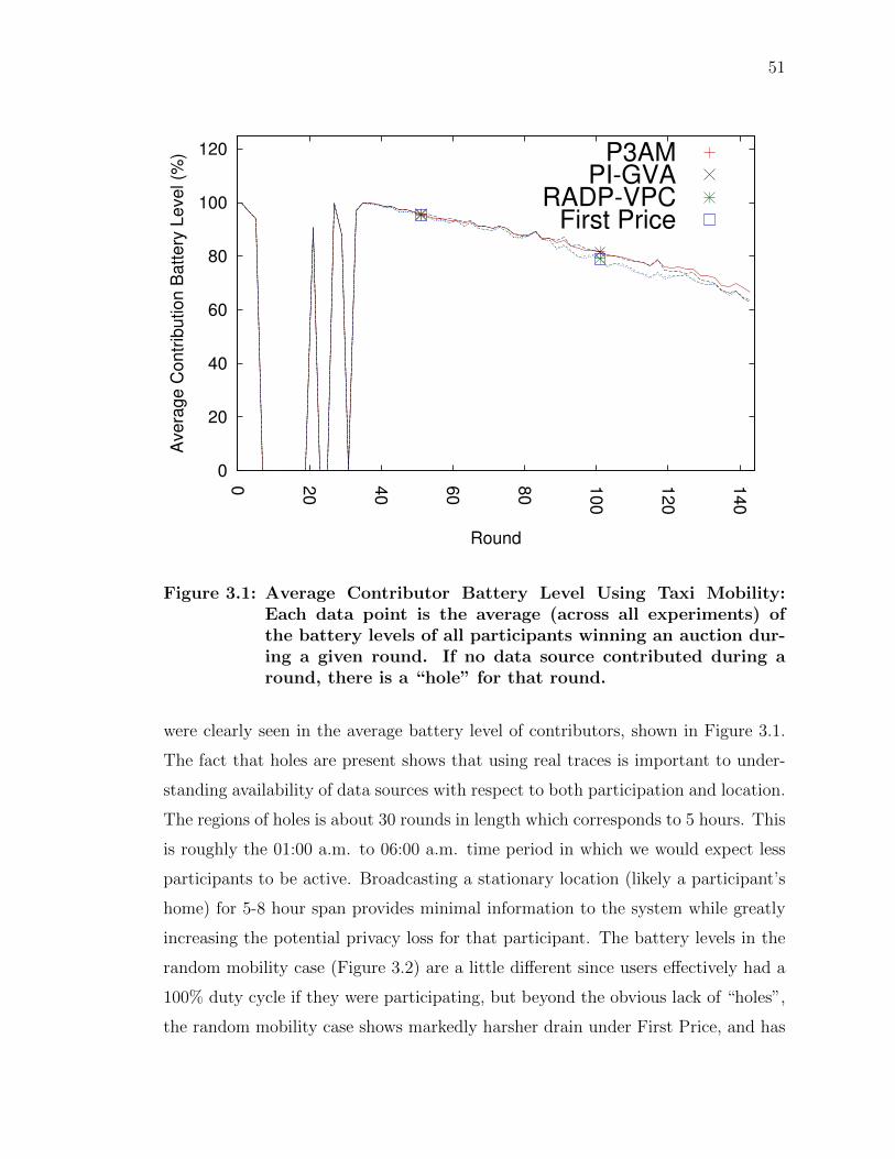
51
0
20
40
60
80
100
120
0 20
40
60
80
100
120
140
Avera
ge C
ontr
ibution B
attery
Level (%
)
Round
P3AMPI-GVA
RADP-VPCFirst Price
Figure 3.1: Average Contributor Battery Level Using Taxi Mobility:Each data point is the average (across all experiments) ofthe battery levels of all participants winning an auction dur-ing a given round. If no data source contributed during around, there is a “hole” for that round.
were clearly seen in the average battery level of contributors, shown in Figure 3.1.
The fact that holes are present shows that using real traces is important to under-
standing availability of data sources with respect to both participation and location.
The regions of holes is about 30 rounds in length which corresponds to 5 hours. This
is roughly the 01:00 a.m. to 06:00 a.m. time period in which we would expect less
participants to be active. Broadcasting a stationary location (likely a participant’s
home) for 5-8 hour span provides minimal information to the system while greatly
increasing the potential privacy loss for that participant. The battery levels in the
random mobility case (Figure 3.2) are a little different since users effectively had a
100% duty cycle if they were participating, but beyond the obvious lack of “holes”,
the random mobility case shows markedly harsher drain under First Price, and has

52
0
20
40
60
80
100
120
0 100
200
300
400
500
600
700
800
900
Avera
ge C
ontr
ibution B
attery
Level (%
)
Tick
P3AMPI-GVA
RADP-VPCFirst Price
Figure 3.2: Average Contributor Battery Level Using Random Mobility:Each data point is the average (across all experiments) of thebattery levels of all participants winning an auction during agiven round. This figure was published at the time of our firststudy in [48], and reflected Dataset II (showing the impactof tolerance to losses).
a crossing point between RADP-VPC and PI-GVA that is absent in the taxi mo-
bility case. These observations indicate that the use of taxi traces as a model of
human mobility for populous regions is realistic, and highlights the importance of
understanding human mobility when designing a participatory sensing system.
Even with extremely low payout settings and very intolerant ROI β, less than
5% of simulated participants stopped participating due to ROI limitations during
the course of the experiments. As a result, the battery level behavior, average price
per measurement and number of samples collected were dependent primarily on
data source movement. Unlike the random mobility case where various parameters
in mechanisms had effects on behavior, the only effect seen in the trace-based ex-
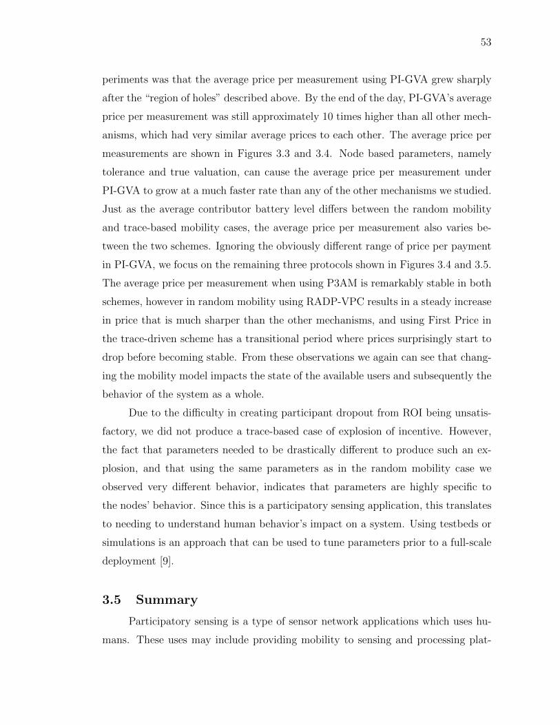
53
periments was that the average price per measurement using PI-GVA grew sharply
after the “region of holes” described above. By the end of the day, PI-GVA’s average
price per measurement was still approximately 10 times higher than all other mech-
anisms, which had very similar average prices to each other. The average price per
measurements are shown in Figures 3.3 and 3.4. Node based parameters, namely
tolerance and true valuation, can cause the average price per measurement under
PI-GVA to grow at a much faster rate than any of the other mechanisms we studied.
Just as the average contributor battery level differs between the random mobility
and trace-based mobility cases, the average price per measurement also varies be-
tween the two schemes. Ignoring the obviously different range of price per payment
in PI-GVA, we focus on the remaining three protocols shown in Figures 3.4 and 3.5.
The average price per measurement when using P3AM is remarkably stable in both
schemes, however in random mobility using RADP-VPC results in a steady increase
in price that is much sharper than the other mechanisms, and using First Price in
the trace-driven scheme has a transitional period where prices surprisingly start to
drop before becoming stable. From these observations we again can see that chang-
ing the mobility model impacts the state of the available users and subsequently the
behavior of the system as a whole.
Due to the difficulty in creating participant dropout from ROI being unsatis-
factory, we did not produce a trace-based case of explosion of incentive. However,
the fact that parameters needed to be drastically different to produce such an ex-
plosion, and that using the same parameters as in the random mobility case we
observed very different behavior, indicates that parameters are highly specific to
the nodes’ behavior. Since this is a participatory sensing application, this translates
to needing to understand human behavior’s impact on a system. Using testbeds or
simulations is an approach that can be used to tune parameters prior to a full-scale
deployment [9].
3.5 Summary
Participatory sensing is a type of sensor network applications which uses hu-
mans. These uses may include providing mobility to sensing and processing plat-

54
0
1
2
3
4
5
6
0 20
40
60
80
100
120
140
Avera
ge C
ost P
er
Measure
ment
Round
P3AMPI-GVA
RADP-VPCFirst Price
Figure 3.3: Average Price per Measurement, Taxi Mobility: Each pointis the average across all experiments of the incentive awardedin exchange for a sample, regardless of if the sample was ata point of interest or not.
forms (by carrying hardware), acting as senors and processors (by deciding when
to submit a report or by annotating data), and designing policies for sensor sys-
tems. Designing a system that involves human participation requires understanding
challenges that arise because of human behavior such as patterns in mobility and
difficulties in maintaining involvement.
Between Section 2.1 and this chapter we have discussed only a sampling of the
existing literature to explore some of the lessons in designing participatory sensing
applications. The increased availability of powerful and versatile mobile hardware,
coupled with a wide array of potential applications suggest great potential for growth
in the field. Designing systems requires an understanding of the application, and
making design decisions about various challenges, such as those described through-
out Section 3.2. While our focus has been on incentivizing systems to maintain

55
0
0.05
0.1
0.15
0.2
0.25
0.3
0.35
0.4
0 20
40
60
80
100
120
140
Avera
ge C
ost P
er
Measure
ment
Round
P3AMRADP-VPC
First Price
Figure 3.4: Average Price per Measurement Zoomed In, Taxi Mobility:Each point is the average across all experiments of the incen-tive awarded in exchange for a sample, regardless of if thesample was at a point of interest or not. This is a zoomedin view of Figure 3.3 to compare P3AM, RADP-VPC, andfirst-price mechanisms
participation, a real-world deployment requires addressing many issues and combin-
ing work done in a variety of independent problems. As the topic of participatory
sensing becomes more popular and more mature, we expect to see more effective
systems that are more advanced and find innovative ways to address the multitude
of design challenges.
Our contributions specifically include a design that is independent of a partic-
ipatory sensing simulation, and the P3AM reverse-auction mechanism, which whose
novelty was incorporating human concerns into the auction mechanism despite the
increased overhead to sensing task operators. Our review of existing work on a va-
riety of aspects guided our design decisions and indicated that such a deployment
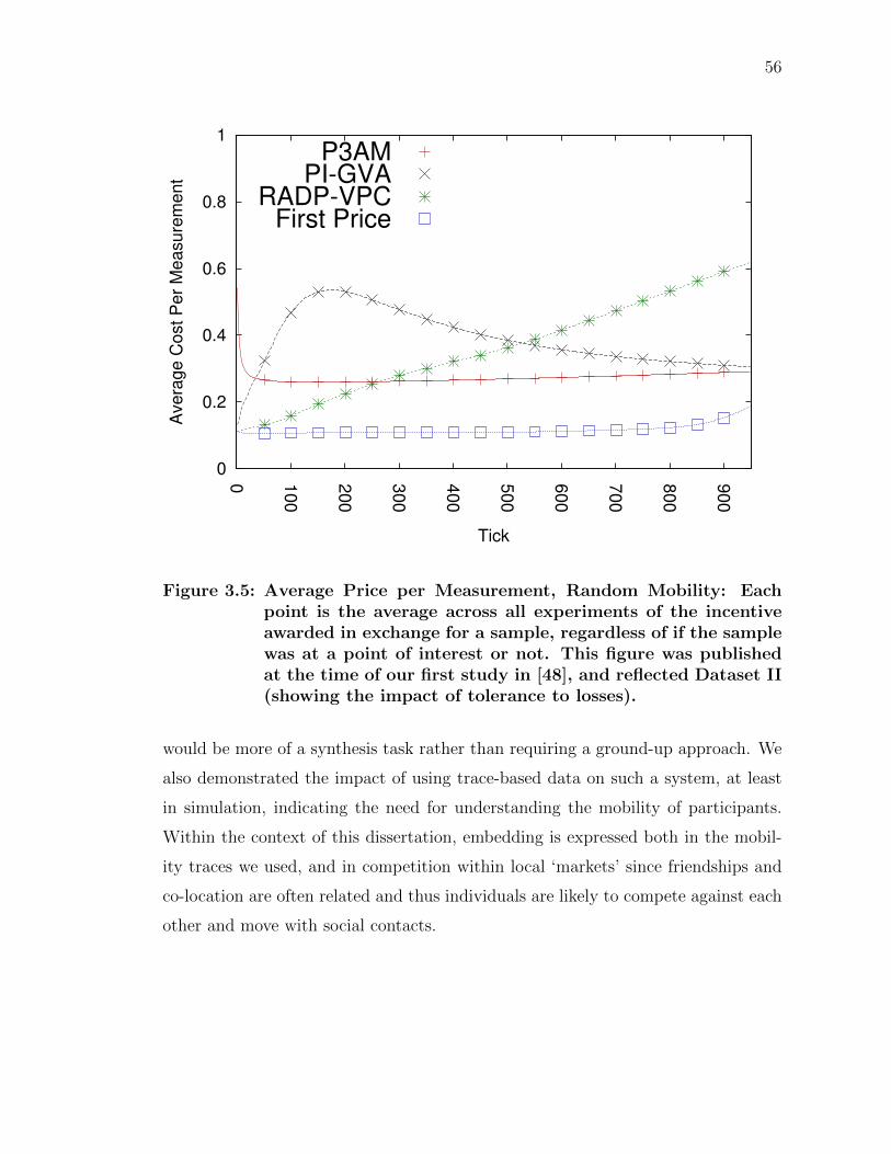
56
0
0.2
0.4
0.6
0.8
1
0 100
200
300
400
500
600
700
800
900
Avera
ge C
ost P
er
Measure
ment
Tick
P3AMPI-GVA
RADP-VPCFirst Price
Figure 3.5: Average Price per Measurement, Random Mobility: Eachpoint is the average across all experiments of the incentiveawarded in exchange for a sample, regardless of if the samplewas at a point of interest or not. This figure was publishedat the time of our first study in [48], and reflected Dataset II(showing the impact of tolerance to losses).
would be more of a synthesis task rather than requiring a ground-up approach. We
also demonstrated the impact of using trace-based data on such a system, at least
in simulation, indicating the need for understanding the mobility of participants.
Within the context of this dissertation, embedding is expressed both in the mobil-
ity traces we used, and in competition within local ‘markets’ since friendships and
co-location are often related and thus individuals are likely to compete against each
other and move with social contacts.

CHAPTER 4
Using Social Interactions as Predictors of Success
4.1 Motivation and Background
Studies in economic sociology suggest that peer-to-peer human relationships
affect economic opportunities because information about these opportunities often
spread most effectively between people [52–58]. Information spreading via interper-
sonal relationships is often richer than traditional broadcast media such as television,
newspaper, radio, etc. because acquaintances can interact face-to-face, provide rel-
evant information when needed, and influence one another with respect to adopting
new behavior and ideas [59].
It has been argued that information coming from weak ties is often richer
than information arriving via strong ties because “those to whom we are weakly
tied are more likely to move in circles different from our own . . . and have access
to information different from what we [usually] receive [56].” Weak ties have been
shown to be valuable sources of information because individuals can use them to
find jobs [52,55], solicit feedback on starting new ventures [58], and search for peo-
ple like in the small-world experiment [60–63]. In other settings such as examining
workplaces, social network structure can affect productivity and innovation of em-
ployees and could lead to higher compensation, more promotion opportunities, and
better performance evaluations [53, 54, 57, 58]. Therefore, the effect of weak ties on
economic opportunities suggests that perhaps the number and distribution of social
ties might also be used for measuring economic development on a larger scale.
Contemporary research on urban characteristics and growth has demonstrated
scaling laws for innovation and wealth creation as a power function of the popula-
tion size as expressed by the equation: y(t) = cx(t)m where x(t) is the population
size and y(t) is the metric of innovation at time t [64, 65]. These results show that
as the population size increases, GDP, wages, patents, private research employment
Portions of this chapter previously appeared as: B. O. Holzbauer, B. K. Szymanski, T. Nguyen,and A. Pentland, “Social ties as predictors of economic development,” in Int. Conf. School NetworkSci., Wroc law, Poland, 2016, pp. 178–185.
57

58
and development increase at superlinear rates where 1.03 ≤ m ≤ 1.46 [65]. Per-
haps the best explanation for the superlinear scaling of wealth creation is that as
the population size increases, the density of social relationships between people in-
creases because there are more choices for establishing relationships [66]; therefore,
increasing the connectivity between people decreases the time for ideas to spread.
Following this line of thinking, recent results in [66] suggest that a generative
model for tie formation as a function of social tie density yields somewhat better
results than purely descriptive models based only on population size, and in ad-
dition offers a simple causal theory of these scaling phenomena. Results obtained
under modest assumptions (nodes distributed uniformly on a Euclidean space, con-
nections established following the rank friendship model [62]) show that algorithmi-
cally generated social ties based on social tie density can be used to model urban
characteristics of cities such as GDP, number of patents, research employment, etc.
Here we extend this line of thinking by focusing on characteristics of economic
development as a function of idea flow based on peer-to-peer social relationships and
find that ”long ties” (defined below) are a main component enabling such flow. This
was accomplished by using data containing geographical locations and friendship
information of hundreds of thousands of people from location-based social media,
namely Gowalla [67]. Also, these datasets allow us to infer face-to-face interactions
[68] and measure the strength of ties in terms of not only interactions but also
geographical and “administrative” distances (i.e., short or long ties [69,70]).
Other approaches for measuring economic development of large geographical
areas include examining the diversity of social contacts (i.e., call detail records as a
proxy for social relationships) since more contacts imply more channels for receiving
information [71]. Yet using calling patterns to infer social contacts is biased towards
those that are more likely to be connected via strong ties since weak ties are by def-
inition those that are used infrequently. While these approaches [66, 71] can vary
in their methodologies, ranging from mathematically oriented to data-driven, what
they share in common is using social network analysis to predict innovation, wealth
creation, and other patterns of complex human behavior. Yet other approaches in-
volve looking more directly at data such as trade [72]. In this chapter, the novelty of

59
our approach lies at the intersection of economic sociology (i.e., the interplay of long
ties and economic opportunities) and simple contagion models (i.e., the spread of
ideas from one place to another). Results show that the speed of access to ideas is a
strongly correlated with social diversity and also a signature of the economic devel-
opment of US states without needing to tune parameters or incorporate secondary
factors such as the level of educational attainment and internal transportation in-
frastructure.
4.2 Data
Our primary focus in this chapter is the Gowalla dataset collected by Ngyuen
and Szymanski, detailed in [67]. The reasoning behind using Gowalla is that a
location-based social network allowed us to analyze both social interactions and
geographic interactions separately (through friendships and check-ins respectively).
We considered specifically applying the network towards modeling United States
(US) Gross Domestic Product (GDP) [73], patents [74], and small startups (20 or
less employees) [75], so we removed any users and corresponding friendship links
that were not internal to the United States. This left us with 75,803 users, 232,278
“long ties” (defined as friendships where the two users were in different physical U.S.
states), and 222,072 “short ties” (friendships where users were in the same state).
In Figure 4.1 we show the hubs (Gowalla user population ≥ 750) which account for
over 90% of users on a map where each point is from a grid with interspacing of
70km, and a user contributes to a point if they are within 50km of it.
While we describe idea flow in more depth in Section 4.3.1, we note now that
by examining correlations between GDP, Patents, Startups, and idea flow, we found
a near-perfect match between correlations using long ties and simulated idea flow.
These correlations are among those presented in Table 4.2. For this reason, we
elected to do the rest of our analysis and discussion here using long ties as a proxy
for idea flow. This is advantageous since long ties can be observed directly from the
network structure, so there is less uncertainty in the accuracy of analysis based on
long ties. For a given state i, we define its census population as Pi, the number of
long ties Li as the number of ties with one end in another state, and the number of
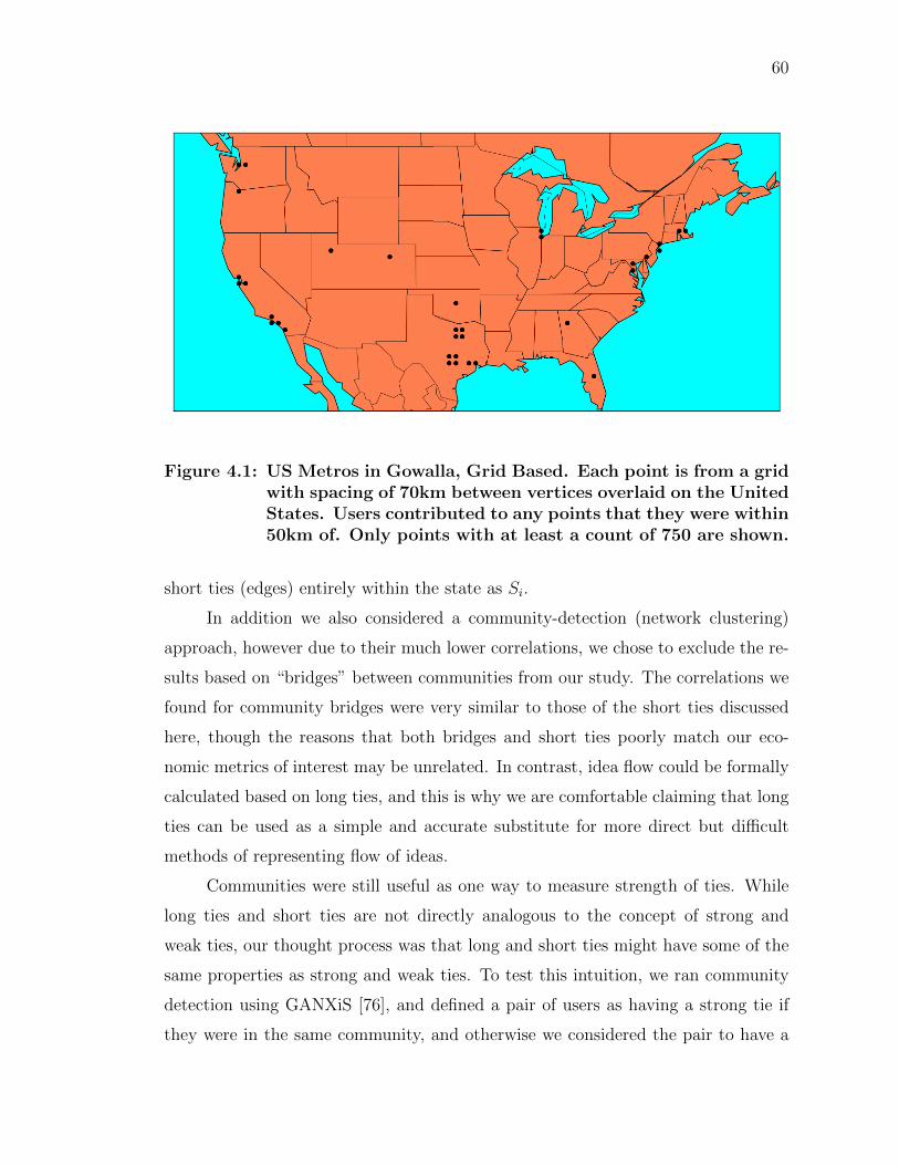
60
Figure 4.1: US Metros in Gowalla, Grid Based. Each point is from a gridwith spacing of 70km between vertices overlaid on the UnitedStates. Users contributed to any points that they were within50km of. Only points with at least a count of 750 are shown.
short ties (edges) entirely within the state as Si.
In addition we also considered a community-detection (network clustering)
approach, however due to their much lower correlations, we chose to exclude the re-
sults based on “bridges” between communities from our study. The correlations we
found for community bridges were very similar to those of the short ties discussed
here, though the reasons that both bridges and short ties poorly match our eco-
nomic metrics of interest may be unrelated. In contrast, idea flow could be formally
calculated based on long ties, and this is why we are comfortable claiming that long
ties can be used as a simple and accurate substitute for more direct but difficult
methods of representing flow of ideas.
Communities were still useful as one way to measure strength of ties. While
long ties and short ties are not directly analogous to the concept of strong and
weak ties, our thought process was that long and short ties might have some of the
same properties as strong and weak ties. To test this intuition, we ran community
detection using GANXiS [76], and defined a pair of users as having a strong tie if
they were in the same community, and otherwise we considered the pair to have a

61
Table 4.1: Summary of Geographic Ties and Strength-Based Ties
Total Short 222072 Total Short and Weak 154066Total Long 232278 Total Long and Weak 180975% of Short Ties that are Weak 69.38 % of Ties that are Weak 73.74% of Long Ties that are Weak 77.91 % of Ties that are Long 51.12
weak tie. We summarize information about ties in the Gowalla component that we
use in Table 4.1; clearly, nearly the same fractions of short and long ties are weak
and close to the fraction of weak ties among all ties. Since, as we show later, long
ties perform better than short ones, we expect that long ties will also outperform
weak ties as predictors of economic metrics.
4.3 Methods
In this section we describe the methodology behind two of the parameters
we considered, idea flow (Section 4.3.1) and social diversity (Section 4.3.2), then
we go into a great deal of detail on how we used our indicators to estimate both
exponential (Section 4.3.3) and Gaussian (Section 4.3.4) and the historical metric
data versus predictions yielded by the models.
4.3.1 Idea Flow
Since we were focused on the idea of innovation being a key factor in growth of
metrics, we believed that examining some form of flow based on the network’s links
would be a promising indicator. The thought behind this was that if innovation
comes from an outside source, we are interested in how long it takes for the idea
to get from any one state to others. By examining the flow or “rate of export” of
ideas, we could create another quantifiable indicator for each state. To calculate
this, we simply ran a random walk simulation starting in each state and running for
10,000,000 steps. We then counted how many steps were between arrivals of each
state, and this gave us the natural flow inter-arrival parameter, λ. Our measure-
ment of flow delay (propagation time) is simply 1λ. To determine the probability
of moving from state i to state j, we used defined a tie-driven probability, fij from

62
literature [77]:
fij =LT (Ai, Aj)∑nk=1 LT (Ai, Ak)
(4.1)
In Equation 4.1, n is the total number of states and LT (Ai, Aj), 1 ≤ i 6=j ≤ m is the number of long ties between states i and j. In other words, fij is
simply the fraction of all long ties from state i that are ties with state j. The idea
flow formulation was previously applied [77], but since the flow matrix from that
experiment was unavailable, we independently constructed a random walk and ran
our own experiments to get the correlations presented in Section 4.4. Our results
were similar but not identical to the previously reported numbers for flow. Because
of the role long ties play in flow and the subsequent random walk, we are not
surprised that long ties and idea flow have similar correlations to GDP, Patents,
and Startups.
4.3.2 Social Diversity
Another idea which Nguyen had previously investigated in his Ph. D. the-
sis [77], was social diversity. The formulation was adapted from existing litera-
ture [71], but the calculations done by Nguyen in [77] were preliminary. Based
on correspondence and independent verification, we found those calculations to be
overly optimistic. The final values we obtained did not indicate a strong correlation
with metrics, but ultimately lead us to examine long and short ties more seriously.
The social diversity Di of state i is defined as follows:
Di =−∑n
j=1 (pij·log(pij))
log(n)(4.2)
In Equation 4.2, pij is the fraction of all edges leaving state i that are long
ties between states i and j. When we examined these values, they performed very
inconsistently, with some having positive correlation and others having negative
correlation. When we revised pij to be a ratio of LT (Ai, Aj) to all ties in state i, we
got results that were still poorly correlated, but consistent and consistently higher
than the original formulation proposed by Nguyen [77]. Despite this improvement,

63
we still chose to not to use social diversity since it still had a correlation value of
less than 0.5.
4.3.3 Estimation of the Exponential Distribution
In order to assess the fitness and significance of our indicators, we fit each of
them to a probability distribution where x1, x2, . . . , xn represents a series of historical
metric data. We start with the well known exponential probability distribution
defined as:
f(x;u) =1
µe
−xµ , 0 < x <∞, 0 < µ <∞ (4.3)
We have anywhere from one to three parameters, namely p, l, and s, which
represent weights to give to each state i’s corresponding population value Pi, long tie
count Li, and short tie count Si. We encode these parameters into the distribution,
along with a corrective constant c by making the mean a linear combination of these
indicators:
µi = p·Pi + l·Li + s·Si + c (4.4)
In the event that a model does not include a parameter, the corresponding
parameter is simply set to 0. Given this probability distribution, the question be-
comes how to evaluate the likelihood that the distribution would yield our histor-
ically known metric data, given a particular set of indicator parameters and the
historical indicator data. We define the likelihood function L as:
L(x1, x2, . . . , xn, p, l, s, c) =n∏i=1
1
µie
−xiµi (4.5)
Since we will be solving the optimization problem of fitting parameters to
maximize likelihood, we find it more convenient to work with sums for differentiation.
Thus, we primarily consider the log-likelihood function:
ln(L) = −n∑i=1
(ln(µi) +
xiµi
)(4.6)

64
Substituting Equation 4.4 into the above equation we get:
ln(L) = −n∑i=1
(ln(p·Pi + l·Li + s·Si + c) +
xip·Pi + l·Li + s·Si + c
)(4.7)
Differentiating through simple application of the chain rule, we get:
∂ln(L)
∂p= −
n∑i=1
(Pi
p·Pi + l·Li + s·Si + c
)−
n∑i=1
(xi·Pi
(p·Pi + l·Li + s·Si + c)2
)∂ln(L)
∂p= −
n∑i=1
(Piµi− xi·Pi
µ2i
)∂ln(L)
∂p= −
n∑i=1
(Pi·µiµ2i
− xi·Piµ2i
)∂ln(L)
∂p= −
n∑i=1
(Pi·
µi − xiµ2i
)(4.8)
We can differentiate Equation 4.7 with respect to the remaining parameters
and obtain results similar to those of Equation 4.8:
∂ln(L)
∂l= −
n∑i=1
(Li·
µi − xiµ2i
)(4.9)
∂ln(L)
∂s= −
n∑i=1
(Si·µi − xiµ2i
)(4.10)
∂ln(L)
∂c= −
n∑i=1
µi − xiµ2i
(4.11)
The problem now becomes how to find extrema of the likelihood function,
whether or not they end up being global. Since we have constrained the domain
to x > 0, the log operation is monotonic so finding extrema of the log-likelihood
via zeroes of the derivatives will indicate parameter values that also minimize (or

65
maximize) the likelihood. We consider three different methods under which we can
select initial points in Sections 4.3.3.1 to 4.3.3.3, and then describe a method to
iteratively solve for roots via gradient descent in Section 4.3.3.4.
4.3.3.1 Method #1: Approximation
It is unlikely that the distribution will exactly fit our linear mean as described
in Equation 4.4, so we instead accept that we are looking at an approximation and
add an additional divergence term, di to reflect this:
µi = xi(1 + di), |di| =|µi − xi|
xi� 1 (4.12)
We can then take an approximation by looking at the first three terms of the
Taylor expansion:
xiµi
=xi
xi(1 + di)≈ 1− di + d2i (4.13)
Equation 4.12 and Taylor expansion also leads us to the following. Note that
if |di| � 1 is not true, this approximation will not hold:
ln(1 + di) = di −1
2d2i (4.14)
Returning to Equation 4.6 and substituting in the definition from Equation 4.12,
we get:
ln(L) = −n∑i=1
(ln(xi·(1 + di)) +
xiµi
)(4.15)
ln(L) = −n∑i=1
(ln(xi) + ln(1 + di)) +
xiµi
)(4.16)
Now using Equation 4.14, we can substitute and get:
ln(L) = −n∑i=1
(ln(xi) + di −
1
2d2i +
xiµi
)(4.17)

66
Adding 1− 1 + 12d2i − 1
2d2i we can group terms together to get:
ln(L) = −n∑i=1
(ln(xi)− (1− di + d2i ) +
xiµi
+ 1 +1
2d2i
)(4.18)
Using the approximation from Equation 4.12 this simplifies to:
ln(L) = −n∑i=1
(ln(xi)−
xiµi
+xiµi
+ 1 +1
2d2i
)ln(L) = −
n∑i=1
(ln(xi) + 1 +
1
2d2i
)(4.19)
Since the unit addition is independent of i we can extract it from the sum.
Rewriting the remaining sum as two separate sums, we arrive at our approximate
log likelihood:
ln(L) = −n−n∑i=1
ln(xi)−n∑i=1
1
2d2i (4.20)
Again, our goal now becomes minimizing the likelihood by finding roots of
the derivatives. Rearranging terms in Equation 4.12, di = µixi− 1, which can be
substituted into Equation 4.20:
ln(L) = −n−n∑i=1
ln(xi)−n∑i=1
1
2
(µixi− 1
)2
∂ln(L)
∂p=
∂
∂p
(−
n∑i=1
1
2
(µixi− 1
)2)
∂ln(L)
∂p= −
n∑i=1
2·12·Pixi
(µixi− 1
)∂ln(L)
∂p= −
n∑i=1
Pixi
(µixi− 1
)(4.21)
Similarly, we can apply the same steps to find the remaining derivatives:

67
∂ln(L)
∂l= −
n∑i=1
Lixi
(µixi− 1
)∂ln(L)
∂s= −
n∑i=1
Sixi
(µixi− 1
)∂ln(L)
∂c= −
n∑i=1
1
xi
(µixi− 1
)(4.22)
This gives us a linear system of equations to solve:
n∑i=1
PiPix2i
PiLix2i
PiSix2i
Pix2i
LiPix2i
LiLix2i
LiSix2i
Lix2i
SiPix2i
SiLix2i
SiSix2i
Six2i
Pix2i
Lix2i
Six2i
1x2i
p
l
s
c
=
−Pixi
−Lixi
−Sixi
− 1xi
(4.23)
Solving a linear system of equations is a well-known problem. In our case we
used Gauss-Jordan elimination with pivoting to solve the system, since this is a
simple and popular solution. However, any method of solving a system of equations
could be used. As long as the matrix is invertible and no linear dependencies are
present, the solution naturally yields the initial parameters pa, la, sa, and ca since
the result is in the form:
1 0 0 0
0 1 0 0
0 0 1 0
0 0 0 1
p
l
s
c
=
pa
la
sa
ca
(4.24)
4.3.3.2 Method #2: Zeroing Parameters
We cannot start with all parameters at 0, since this would cause µi = 0, and
Equation 4.3 by definition requires a positive µi value. However, we can set all
parameters to 0 except c, and consider this as an additional starting point. If this
is the case c must be selected carefully, since a poorly chosen initial condition may
result in a gradient descent to a needlessly sub-optimal solution. Considering this

68
arrangement, the log-likelihood function is:
ln(L) = −n∑i=1
(ln(c) +
xic
)(4.25)
Since the goal is still optimization, we again take the derivative. This time
there is only one independent variable, so we can eschew use of the partial derivative
symbol:
dln(L)
dc=
n∑i=1
(1
c− xic2
)dln(L)
dc=
1
c
n∑i=1
(1− xi
c
)dln(L)
dc=
1
c
(n− 1
c
n∑i=1
xi
)(4.26)
The root of the derivative is then at:
0 =1
c
(n− 1
c
n∑i=1
xi
)
0 = n− 1
c
n∑i=1
xi
n =1
c
n∑i=1
xi
c =
∑ni=1 xin
(4.27)
This is an intuitive solution for µc,0i = c, since µi in the exponential distri-
bution is the average (expectation) value. Thus, our second initial condition is all
parameters set to 0 except c =∑ni=1 xin
.
4.3.3.3 Method #3: Mixed Solutions
A third possibility for initial conditions is mixing weights from different models.
In the case of models with only a single indicator, we instead mix between µc,0i and

69
for indicator k ∈ {p, l, s}, µk,0i . To begin with, we define µk,0i which can be derived
in a similar manner to how we found µc,0i in Equations 4.25-4.27:
µp,0i =
∑ni=1
xiPi
n(4.28)
µl,0i =
∑ni=1
xiLi
n(4.29)
µs,0i =
∑ni=1
xiSi
n(4.30)
We then define a mixture weight b ∈ [0, 1] where the initial starting point will
be k = b·ka (where ka is the approximate solution from 4.24), and c = (1 − b)·ca.To solve for b, we once again look at the log-likelihood function, but with our new
k and c values. Here, we denote Ki as the corresponding state-dependent variable
that k influences:
ln(L) = −n∑i=1
(ln(b·ka·Ki + (1− b)·ca) +
xib·ka·Ki + (1− b)·ca
)(4.31)
The derivative with respect to b (the parameter we want to optimize) is:
ln(L)
db= −
n∑i=1
(ka·Ki − ca
b·ka·Ki + (1− b)·ca
(1− xi
b·ka·Ki + (1− b)ca
))(4.32)
Setting Equation 4.32 to 0, we can solve for the optimal value of b. Since this
equation is non-linear we used MATLAB to find a solution.
For the models with two parameters, namely PS, PL, and SL, we consider
the two parameters j and k, and their optimal solutions in the respective single
model cases, µji = jopt + cj and µki = kopt + ck. Note that these two solutions both
contain separate constants cj and ck, which do not have to match. We then write
a likelihood function with weight b, where our initial conditions will be j = b·jopt,

70
k = (1− b)·kopt, and c = b·cj + (1− b)·ck:
ln(L) = −n∑i=1
(ln(b·µj + (1− b)·µk) +
xib·µj + (1− b)·µk
)(4.33)
The derivative with respect to b is then:
ln(L)
db= −
n∑i=1
(µj − µk
b·µj + (1− b)·µk
(1− xi
b·µj + (1− b)µk
))(4.34)
Finding the root of the derivative again gives us the optimal b value for mixing
the two models, and this can be solved the same way the single parameter derivative
could.
Finally, we consider the case of PLS, which uses all three parameters. In
this case, we still keep one weight, b, and simply consider three pairs of models:
(j, k) ∈ {(PS, L), (PL, S), (LS, P )}. The analysis then can be carried out exactly
as written above for the two parameter case, with the simple change that µj =
j(1)opt·J
(1)i + j
(2)opt·J
(2)i + cj, where j(1) is the first variable in the two parameter model
j represents, and j(2) is the second variable. We can then set j(1) = b·j(1)opt and
j(2) = b·j(2)opt. Using this notation, the remaining parameter k, and the constant c
are still calculated as in the two parameter model.
4.3.3.4 Iteration on Parameters
While the starting points we have described in Sections 4.3.3.1 - 4.3.3.3 are
educated guesses as to where extreme will exist, they are not guaranteed to actually
be extrema. From these initial conditions, we iteratively perform a gradient descent,
in which we either stop when |∆ln(L)| < 0.001 or the iteration moves us in the wrong
direction (i.e. increases |ln(L)|) since this indicates a point of inflection that will
move the parameters towards larger error.
Each of the parameters forms a dimension in the search space, so we must

71
examine the partial derivatives for each parameter. For simplicity, we define:
y(p, l, s, c) = ln(L)
y′p =∂ln(L)
∂p
y′′p,l =∂
∂l
∂ln(L)
∂p
The first derivatives were already defined earlier in Equations 4.8 - 4.11, but
we must now define the second derivatives. They are:
y′′p,p =n∑i=1
(Pi·Piµ2i
(1− 2·xi
µi
))y′′p,l =
n∑i=1
(Pi·Liµ2i
(1− 2·xi
µi
))y′′p,s =
n∑i=1
(Pi·Siµ2i
(1− 2·xi
µi
))y′′p,c =
n∑i=1
(Piµ2i
(1− 2·xi
µi
))(4.35)
y′′l,p =n∑i=1
(Li·Piµ2i
(1− 2·xi
µi
))y′′l,l =
n∑i=1
(Li·Liµ2i
(1− 2·xi
µi
))y′′l,s =
n∑i=1
(Li·Siµ2i
(1− 2·xi
µi
))y′′l,c =
n∑i=1
(Liµ2i
(1− 2·xi
µi
))(4.36)

72
y′′s,p =n∑i=1
(Si·Piµ2i
(1− 2·xi
µi
))y′′s,l =
n∑i=1
(Si·Liµ2i
(1− 2·xi
µi
))y′′s,s =
n∑i=1
(Si·Siµ2i
(1− 2·xi
µi
))y′′s,c =
n∑i=1
(Siµ2i
(1− 2·xi
µi
))(4.37)
y′′c,p =n∑i=1
(Piµ2i
(1− 2·xi
µi
))y′′c,l =
n∑i=1
(Liµ2i
(1− 2·xi
µi
))y′′c,s =
n∑i=1
(Siµ2i
(1− 2·xi
µi
))y′′c,c =
n∑i=1
(1
µ2i
(1− 2·xi
µi
))(4.38)
Finally, we can define step t of the iteration as having p(t), l(t), s(t), and c(t),
with t = 1 being the first step and having the initial conditions. We consider the
approximation for the next step, based on changes p(t+1) = p(t)+∆p, l(t+1) = l(t)+∆l,
s(t+1) = s(t) + ∆s, and c(t+1) = c(t) + ∆c:
0 = y′p(p(t+1), l(t+1), s(t+1), c(t+1)) ≈ y′p(p
(t) + ∆p, l(t)∆l, s(t)∆s, c(t) + ∆c)
0 = y′l(p(t+1), l(t+1), s(t+1), c(t+1)) ≈ y′l(p
(t) + ∆p, l(t)∆l, s(t)∆s, c(t) + ∆c)
0 = y′s(p(t+1), l(t+1), s(t+1), c(t+1)) ≈ y′s(p
(t) + ∆p, l(t)∆l, s(t)∆s, c(t) + ∆c)
0 = y′c(p(t+1), l(t+1), s(t+1), c(t+1)) ≈ y′c(p
(t) + ∆p, l(t)∆l, s(t)∆s, c(t) + ∆c) (4.39)
We can then solve the system of equations described in Equation 4.40 to get

73
the parameter values at the next step, and subsequently the log-likelihood as defined
in Equation 4.6:
y′′p,p y′′p,l y′′p,s y′′p,c
y′′l,p y′′l,l y′′l,s y′′l,c
y′′s,p y′′s,l y′′s,s y′′s,c
y′′c,p y′′c,l y′′c,s y′′c,c
∆p
∆l
∆s
∆c
=
−y′p−y′l−y′s−y′c
(4.40)
4.3.4 Estimation of the Gaussian Distribution
Since there was no guarantee that the exponential distribution would be a good
fit, we elected to also consider fitting the data to the commonly used probability
Gaussian distribution:
f(x;µ, σ) =1
σ√
2πe
−(x−µ)2
2σ2 ,−∞ < x <∞, 0 < σ <∞ (4.41)
If we consider indicator X, then by normalizing the distribution to N(1, σnorm),
we can define Xnorm,i = Xiµi
, µnorm,i = µiµi
= 1, and σnorm = σiµi
. The formula for µi is
the same as in Equation 4.4. For readability, we define v = σ2norm, and note that v
is a single value as opposed to having a separate vi for each state.
The likelihood function is more complicated, but can be written as:
L(x1, x2, . . . , xn; p, l, s, c, v) =1
vn2 (2π)
n2
n∏i=1
(1
µie− 1
2v·µ2i
(xi−µi)2)
=e− 1
2v
∑ni=1
(1
µ2i
(xi−µi)2)
vn2 (2π)
n2
n∏i=1
1
µi(4.42)
Taking the log of Equation 4.42 we get the log-likelihood:
ln(L) = −n2lnv − n
2ln(2π)−
n∑i=1
lnµi −1
2v
n∑i=1
(1− xi
µi
)2
(4.43)
To solve for v, we will consider the four partial derivatives of ln(L) (one per
parameter), and since we have five unknowns and need five equations, the fifth
equation will come from the partial derivative of ln(L) with respect to v. We present

74
the resulting equations (after multiplying the first four by v for convenience):
−v∂ln(L)
∂p= v
n∑i=1
Piµi
+n∑i=1
(xiPiµ2i
(1− xi
µi
))(4.44)
−v∂ln(L)
∂l= v
n∑i=1
Liµi
+n∑i=1
(xiLiµ2i
(1− xi
µi
))−v∂ln(L)
∂s= v
n∑i=1
Siµi
+n∑i=1
(xiSiµ2i
(1− xi
µi
))−v∂ln(L)
∂c= v
n∑i=1
1
µi+
n∑i=1
(xiµ2i
(1− xi
µi
))∂ln(L)
∂v= − n
2v+
1
2v2
n∑i=1
(1− xi
µi
)2
We can then multiply ∂ln(L)∂v
by v, and solve for roots (i.e. set ∂ln(L)∂v
= 0) to
get:
v =1
n
n∑i=1
(1− xi
µi
)2
(4.45)
4.3.4.1 Linear Approximation
As in Section 4.3.3.1, we next looked at a linear approximation by introducing
di, where di � 1. Here the approximation is:
µi = xi + di
µi = xi
(1 +
dixi
)(4.46)
We consider Equation 4.44, and look at the two terms separately. We start by
substituting Equation 4.46 into the first term:
vn∑i=1
Piµi
= vn∑i=1
Pi
xi
(1 + di
xi
) (4.47)
Next, substituting Equation 4.46 things get a little more complicated:

75
n∑i=1
(xiPiµ2i
(1− xi
µi
))
=n∑i=1
xiPi(xi
(1 + di
xi
))21− xi
xi
(1 + di
xi
)
=n∑i=1
xiPi
x2i
(1 + di
xi
)21− xi
xi
(1 + di
xi
)
=n∑i=1
Pi· xi
x2i
(1 + di
xi
)2 − x2i
x3i
(1 + di
xi
)3
=n∑i=1
Pi· xi
(1 + di
xi
)x2i
(1 + di
xi
)3 − x2i
x3i
(1 + di
xi
)3
=n∑i=1
Pi· xi
(1 + di
xi
)x2i
(1 + di
xi
)3 − xi
x2i
(1 + di
xi
)3
=n∑i=1
Pi·xi
(1 + di
xi
)− xi
x2i
(1 + di
xi
)3
=n∑i=1
Pi· xi + di − xi
x2i
(1 + di
xi
)3
=n∑i=1
Pi· di
x2i
(1 + di
xi
)3
=n∑i=1
Pi
x2i
(1 + di
xi
)3 ·di (4.48)
Combining the two terms on the right hand side of Equations 4.47 and 4.48,

76
we get:
v
n∑i=1
Pi
xi
(1 + di
xi
) +n∑i=1
Pi
x2i
(1 + di
xi
)3 di (4.49)
Again we use the fact that di is very small to rearrange and drop high-order
di terms:
v
n∑i=1
Pi
xi
(1 + di
xi
) +n∑i=1
Pi
x2i
(1 + di
xi
)3 di
≈ vn∑i=1
(Pixi
(1− di
xi
))+
n∑i=1
(Pix2i·di)
≈ vn∑i=1
(Pixi− Pix2i·di)
+n∑i=1
(Pix2i·di)
≈ vn∑i=1
Pixi− v
n∑i=1
(Pix2i·di)
+n∑i=1
(Pix2i·di)
≈ vn∑i=1
Pixi
+ (1− v)n∑i=1
(Pix2i·di)
(4.50)
Next, since this is an approximation of the derivative and we are interested in
the behavior at roots, we set Equation 4.50 to 0, then use the fact that di = µi− xito solve for a relationship in terms of µi:

77
v
n∑i=1
Pixi
+ (1− v)n∑i=1
(Pix2i·di)
= 0
(1− v)n∑i=1
(Pix2i·di)
= −vn∑i=1
Pixi
n∑i=1
(Pix2i·di)
=−v
(1− v)
n∑i=1
Pixi
n∑i=1
(Pix2i·di)
=v
(v − 1)
n∑i=1
Pixi
n∑i=1
(Pix2i· (µi − xi)
)=
v
(v − 1)
n∑i=1
Pixi
n∑i=1
(Pix2i·µi)−
n∑i=1
(Pix2i·xi)
=v
(v − 1)
n∑i=1
Pixi
n∑i=1
(Pix2i·µi)−
n∑i=1
(Pixi
)=
v
(v − 1)
n∑i=1
Pixi
n∑i=1
(Pix2i·µi)
=v
(v − 1)
n∑i=1
Pixi
+n∑i=1
(Pixi
)n∑i=1
(Pix2i·µi)
=v
(v − 1)
n∑i=1
Pixi
+v − 1
v − 1
n∑i=1
(Pixi
)n∑i=1
(Pix2i·µi)
=v + v − 1
(v − 1)
n∑i=1
Pixi
n∑i=1
(Pix2i·µi)
=2v − 1
(v − 1)
n∑i=1
Pixi
(4.51)
For readability, we then define V = 2v−1v−1 and v = V−1
V−2 , and rewrite Equa-
tion 4.51 accordingly:
n∑i=1
(Pix2i·µi)
= Vn∑i=1
Pixi
(4.52)
Finally, we can substitute Equation 4.4 into Equation 4.52 and repeat the
process for the other partial derivatives (∂ln(L)∂l
, ∂ln(L)∂s
, and ∂ln(L)∂c
) to get:

78
n∑i=1
(Pix2i· (p·Pi + l·Li + s·Si + c)
)= V
n∑i=1
Pixi
n∑i=1
(Lix2i· (p·Pi + l·Li + s·Si + c)
)= V
n∑i=1
Lixi
n∑i=1
(Six2i· (p·Pi + l·Li + s·Si + c)
)= V
n∑i=1
Sixi
n∑i=1
(1
x2i· (p·Pi + l·Li + s·Si + c)
)= V
n∑i=1
1
xi
We can then rewrite this as a system of equations:
n∑i=1
PiPix2i
PiLix2i
PiSix2i
Pix2i
LiPix2i
LiLix2i
LiSix2i
Lix2i
SiPix2i
SiLix2i
SiSix2i
Six2i
Pix2i
Lix2i
Six2i
1x2i
p
l
s
c
=
−Pixi
−Lixi
−Sixi
− 1xi
(4.53)
Finally, we observe that the system described in Equation 4.53 is exactly the
same as Equation 4.23, where the free term in the exponential case is now represented
by the V term. This means that if we solve the exponential case first we know that
the solution for the exponential parameters, denoted as (p(exp)sol , l
(exp)sol , s
(exp)sol , c
(exp)sol ),
will be the solution here as well. We can then scale by V to translate parameters to
the Gaussian space, and get that:
p = V ·pexpsol
l = V ·lexpsol
s = V ·sexpsol
c = V ·cexpsol
µi,a = (p(exp)sol ·Pi + l
(exp)sol ·Li + s
(exp)sol ·Si + c
(exp)sol )V (4.54)
µi,a = µi,solV

79
This µi,a is only used for the initial condition assuming the linear approxima-
tion. We still use Equation 4.4 and not Equation 4.54 for all other calculations, such
as actual likelihood and iteration steps. However, we first apply the approximate
mean to the likelihood function to find an initial v:
ln(L) = −n2ln(v)− n
2ln(2π)−
n∑i=1
ln(µi,sol)− n·ln(
2v − 1
v − 1
)− 1
2v
n∑i=1
(1− v − 1
2v − 1
xiµi,sol
)2
(4.55)
We can then look at the derivative of Equation 4.55 with respect to v to find
the values of v that are roots:
∂ln(L)
∂v= −n(v − 1)
2v2− 2n
2v − 1+
n
v − 1− 2v2 − 4v + 1
v2 (2v − 1)2
n∑i=1
xiµi,sol
+(v − 1) (2v2 − 5v + 1)
2v2 (2v − 1)3
n∑i=1
(xiµi,sol
)2
(4.56)
For simplicity we define two more symbols: X =
∑ni=1
xiµi,sol
nand Y =
∑ni=1
(xi
µi,sol
)2
n.
If we consider dividing Equation 4.56 by n at the zero, and substituting in X and
Y we get:
0 =(v − 1)
2v2+
2
2v − 1− 1
v − 1+
2v2 − 4v + 1
v2 (2v − 1)2X
− (v − 1) (2v2 − 5v + 1)
2v2 (2v − 1)3Y (4.57)
We can then rearrange Equation 4.57 to group by descending degree of v and
define it as a function r(v):

80
r(v) = 8v5+(−36 + 8X − 2Y )v4 + (46− 28X + 9Y )v3 + (−27 + 32X − 13Y )v2
+ (8− 14X + 7Y )v − 1 + 2X − Y (4.58)
Finally, the roots of Equation 4.58 can be solved for. If vvalid = {vj|r(vj) =
0, vj ∈ R, vj > 0}, then the optimal initial value for v is:
v0,opt = argmaxvj∈vvalid
ln(L(x1, x2, . . . , xn; p·vj, l·vj, w·vj, c·vj, vj)) (4.59)
We can then use the following initial conditions:
v = v0,opt
p = pexpsol V
l = lexpsol V
s = sexpsol V
c = cexpsol V (4.60)
4.3.4.2 Iteration on Parameters
Just as in the exponential case, the initial condition is an educated guess
about where in the search space an extrema will exist. However, since it is not
guaranteed that the initial conditions will evaluate to an extrema, we perform an
iterative search using the same stopping conditions as in Section 4.3.3.4. We also
use the same notation for first and second derivatives, but now L is a function of
all 5 parameters: p, l, s, c,and v. However, since we now have a fifth variable v
and a different likelihood function, we once again must define all second derivatives
(Equations 4.61 to 4.65) and the system of equations to iterate upon (Equation 4.66).
We also provide the natural update rule that for iteration t+ 1, v(t+1) = v(t) + ∆v.

81
y′′p,p =n∑i=1
Pi·Piµ2i
+1
v
n∑i=1
(xi·Pi·Piµ3i
(2− 3
xiµi
))y′′p,l =
n∑i=1
Pi·Liµ2i
+1
v
n∑i=1
(xi·Pi·Liµ3i
(2− 3
xiµi
))y′′p,s =
n∑i=1
Pi·Siµ2i
+1
v
n∑i=1
(xi·Pi·Siµ3i
(2− 3
xiµi
))y′′p,c =
n∑i=1
Piµ2i
+1
v
n∑i=1
(xi·Piµ3i
(2− 3
xiµi
))y′′p,v =
1
v2
n∑i=1
(xi·Piµ2i
(1− xi
µi
))(4.61)
y′′l,p =n∑i=1
Li·Piµ2i
+1
v
n∑i=1
(xi·Li·Piµ3i
(2− 3
xiµi
))y′′l,l =
n∑i=1
Li·Liµ2i
+1
v
n∑i=1
(xi·Li·Liµ3i
(2− 3
xiµi
))y′′l,s =
n∑i=1
Li·Siµ2i
+1
v
n∑i=1
(xi·Li·Siµ3i
(2− 3
xiµi
))y′′l,c =
n∑i=1
Liµ2i
+1
v
n∑i=1
(xi·Liµ3i
(2− 3
xiµi
))y′′l,v =
1
v2
n∑i=1
(xi·Liµ2i
(1− xi
µi
))(4.62)

82
y′′s,p =n∑i=1
Si·Piµ2i
+1
v
n∑i=1
(xi·Si·Piµ3i
(2− 3
xiµi
))y′′s,l =
n∑i=1
Si·Liµ2i
+1
v
n∑i=1
(xi·Si·Liµ3i
(2− 3
xiµi
))y′′s,s =
n∑i=1
Si·Siµ2i
+1
v
n∑i=1
(xi·Si·Siµ3i
(2− 3
xiµi
))y′′s,c =
n∑i=1
Siµ2i
+1
v
n∑i=1
(xi·Siµ3i
(2− 3
xiµi
))y′′s,v =
1
v2
n∑i=1
(xi·Siµ2i
(1− xi
µi
))(4.63)
y′′c,p =n∑i=1
Piµ2i
+1
v
n∑i=1
(xi·Piµ3i
(2− 3
xiµi
))y′′c,l =
n∑i=1
Liµ2i
+1
v
n∑i=1
(xi·Liµ3i
(2− 3
xiµi
))y′′c,s =
n∑i=1
Siµ2i
+1
v
n∑i=1
(xi·Siµ3i
(2− 3
xiµi
))y′′c,c =
n∑i=1
1
µ2i
+1
v
n∑i=1
(xiµ3i
(2− 3
xiµi
))y′′c,v =
1
v2
n∑i=1
(xiµ2i
(1− xi
µi
))(4.64)

83
y′′v,p =1
v2
n∑i=1
(xi·Piµ2i
(1− xi
µi
))y′′v,l =
1
v2
n∑i=1
(xi·Liµ2i
(1− xi
µi
))y′′v,s =
1
v2
n∑i=1
(xi·Siµ2i
(1− xi
µi
))y′′v,c =
1
v2
n∑i=1
(xiµ2i
(1− xi
µi
))y′′v,v =
n
2v2− 1
v3
n∑i=1
(1− xi
µi
)2
(4.65)
y′′p,p y′′p,l y′′p,s y′′p,c y′′p,v
y′′l,p y′′l,l y′′l,s y′′l,c y′′l,v
y′′s,p y′′s,l y′′s,s y′′s,c y′′s,v
y′′c,p y′′c,l y′′c,s y′′c,c y′′c,v
y′′v,p y′′v,l y′′v,s y′′v,c y′′v,v
∆p
∆l
∆s
∆c
∆v
=
−y′p−y′l−y′s−y′c−y′v
(4.66)
4.3.5 Short and Long Tie Counting
We were interested in idea flow across state lines since we believe that short ties
are less conducive to innovation due to competition for the same resources. This idea
can be conceptualized in any environment with resources divided by administrative
boundaries, whether it be geographic provinces, states, etc. or a division that isn’t
geographic such as competing for grants across departments in a university or across
universities with a common funding pool.
Our method simply counts the number of ties between states, with long and
short ties defined in Section 4.2. Since ties are based on the relationship, or connec-
tion, between users in the network, the long ties and short ties indicators are just
the numbers of edges that qualify as long or short respectively.
We also consider an indicator inspired by the Adamic-Adar (AA) score [78],
which has been used to provide a weighted frequency count [79]. Unlike AA, for
state i instead of counting long ties, we take the sum of a log2(nk) for all nodes k

84
Table 4.2: Correlations Between Indicators and Economic Metrics
Feature GDP Patents StartupsPopulation .985 .865 .982Long Ties .921 .788 .892Short Ties .692 .531 .599Idea Flow .906 .784 .877Social Diversity .167 .151 .164Bridges .673 .482 .579
that have the number of long ties, nk > 0.
We also evaluated the number of users connected to a user in the given state
which have non-zero count of long ties, which in contrast to our edge-like count
described above, can be viewed as a node-like count. However, both AA-inspired
and the node count indicator had high correlation with state population indicator
(above 90%) and the models combining either of them were statistically similar to
the models with state population alone. This indicates that both indicators were
just proxies of state population, so we did not consider them for further study.
4.4 Results
The first thing we examined was how indicators, including Pi, Li, and Si, cor-
relate with metrics GDPi, Patentsi, and Startupsi. For a given feature (indicator),
the value for state i is correlated to the metric for the same state i. For example,
when looking at the total long ties in state i, some ties will be in another state j 6= i,
a third state k 6= i, j, and so on. The only values this total is correlated to are the
metrics for state i. The results shown in Table 4.2 indicate that population is better
correlated with the metrics then either type of ties, and short ties correlations are
particularly low. For the models we consider, we used leave-one-out cross-validation
and did not see a difference of more than ±0.0005 in correlation.
Such high correlations of total population can arise because either each addi-
tional person adds a similar increment to the network of social relationships and idea
flow, or their individual cognitive processes are generating innovations independent
of their social context. Thus, it is interesting that short ties (within the same state)

85
are relatively less correlated with the metrics, while long ties (between states) have
correlations that are significantly stronger.
We therefore examined Pi, Li, and Si in the context of distributions over
each indicator and computed the probability that state data are drawn from them.
Moreover, we looked how this probability changes as we enrich models by adding
successively more indicators. We considered both the exponential and Gaussian
estimation as described in Sections 4.3.3 - 4.3.4 for each economic metric against
single variables (P ,L,S models), pairs (PL,PS,LS models), and a three-variable
model (PLS) using Maximum Likelihood Estimation (MLE) [80]. This estimation
was computed by approximating the likelihood function derivative solution to zero
and then following the highest gradient descent to the nearest maximum, so we
cannot guarantee that we found the global extrema. For the exponential estimations,
we chose the best value after iterating from each of the three initial conditions,
which was consistently Method #1 described in Section 4.3.3.1, except for PS fit
to GDP which had the best results with Method #3 described in Section 4.3.3.3.
The logs of maximum likelihoods of fitting state data by each model are shown in
Tables 4.3 and 4.4. Thanks to use of more precise methods to estimate optimal
values of parameters compared to our prior work in [81], the results presented in
Table 4.4 are new and led us to more refined conclusions in this dissertation. For
example, in our current work, we chose the best value after iterating from each of
the three starting points for iterations, and each has at least one method for which
this starting point was the best. Still, the MLEs we obtain are not guaranteed to
be global maximum likelihoods since the methods used are not exact solutions.
From examining the likelihood ratios, we can find the probability that the two
nested models are not the same via the Likelihood Ratio Test (LRT) [80]. This is the
case when one models parameters are a subset of the other models parameters. In
this case, a Chi-Square distribution with the degree of freedom equal to the difference
in the number of parameters between the models is used to find confidence level with
which we can conclude that the models are different. For cases where the models
are not nested, we instead apply the Akaike information criterion (AIC) [82].
The AIC score of the model is defined as 2 ∗ ln(L) − 2(p + 1) where L is the
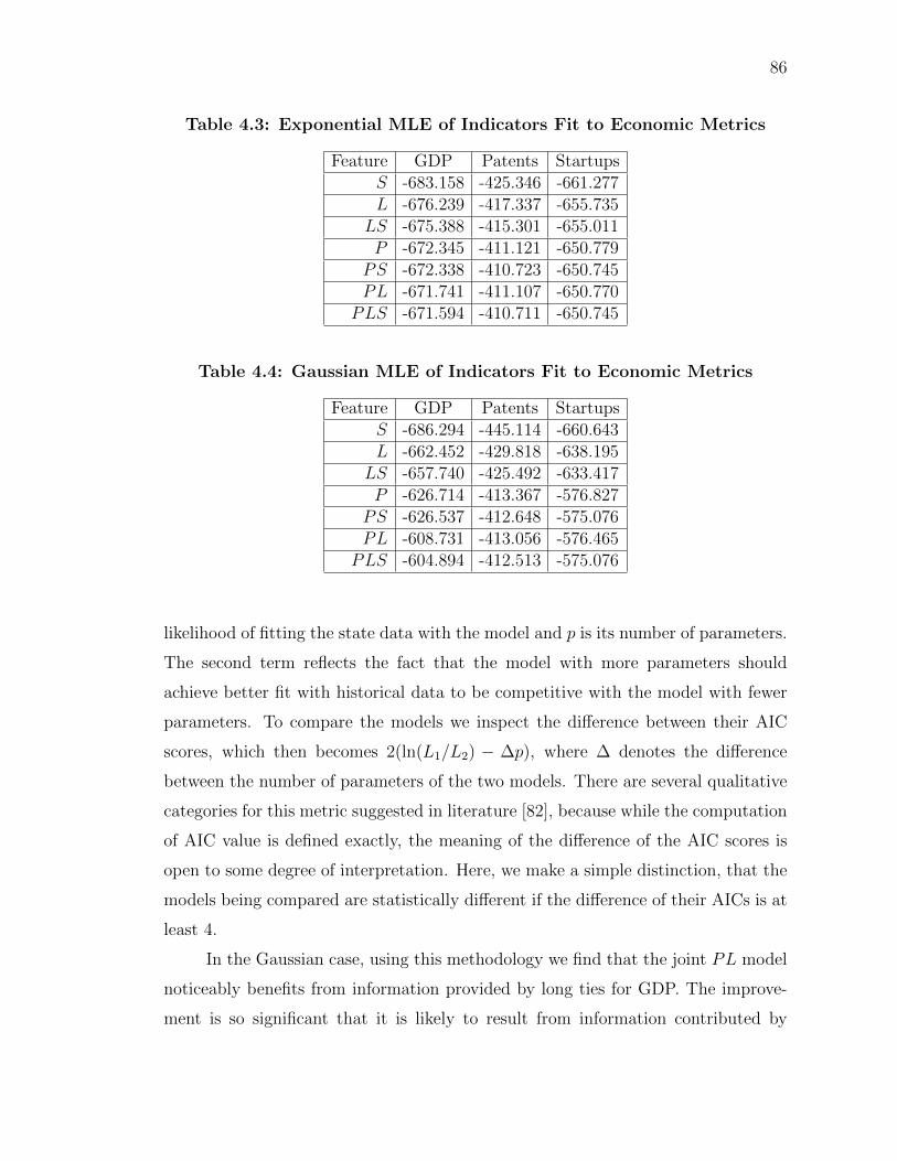
86
Table 4.3: Exponential MLE of Indicators Fit to Economic Metrics
Feature GDP Patents StartupsS -683.158 -425.346 -661.277L -676.239 -417.337 -655.735
LS -675.388 -415.301 -655.011P -672.345 -411.121 -650.779
PS -672.338 -410.723 -650.745PL -671.741 -411.107 -650.770
PLS -671.594 -410.711 -650.745
Table 4.4: Gaussian MLE of Indicators Fit to Economic Metrics
Feature GDP Patents StartupsS -686.294 -445.114 -660.643L -662.452 -429.818 -638.195
LS -657.740 -425.492 -633.417P -626.714 -413.367 -576.827
PS -626.537 -412.648 -575.076PL -608.731 -413.056 -576.465
PLS -604.894 -412.513 -575.076
likelihood of fitting the state data with the model and p is its number of parameters.
The second term reflects the fact that the model with more parameters should
achieve better fit with historical data to be competitive with the model with fewer
parameters. To compare the models we inspect the difference between their AIC
scores, which then becomes 2(ln(L1/L2) − ∆p), where ∆ denotes the difference
between the number of parameters of the two models. There are several qualitative
categories for this metric suggested in literature [82], because while the computation
of AIC value is defined exactly, the meaning of the difference of the AIC scores is
open to some degree of interpretation. Here, we make a simple distinction, that the
models being compared are statistically different if the difference of their AICs is at
least 4.
In the Gaussian case, using this methodology we find that the joint PL model
noticeably benefits from information provided by long ties for GDP. The improve-
ment is so significant that it is likely to result from information contributed by

87
Table 4.5: MLE Differences for Confidence Levels Using LRT (χ2)
Confidence Level: 0.95 0.99 0.999∆Degrees of Freedom = 1: 1.92 3.32 5.50∆Degrees of Freedom = 2: 3.00 4.61 6.90
Table 4.6: Mapping of ∆AIC and χ2 Values to Qualitative Categories.Note that these do not imply an equivalence between ∆AICvalues and χ2 values, but rather are mappings of both criteriainto “Confidence In Similarity.”
Confidence In Difference ∆AIC χ2
Strong ≥10 ≥.99Moderate ≥4, < 10 ≥.95, < 0.99
Weak < 4 < .95
the long ties and not captured by the population alone. In contrast, the difference
of likelihoods between PS model which includes short ties and population-only P
model is not statistically significant for any metric. On the other hand, for all three
metrics LS improves over both L and S models significantly as is L model over S
model. Because of the nearly exact match between long ties and our simulation of
idea flow, the same should be true of other measurements of idea flow. As a sum-
mary, the list of models for which the differences in likelihoods are not statistically
significant is: P and PS models for all metrics, P , PS, PL and PLS for Patents
and Startups.
The exponential case is a little different. Here, the significance of models was
more varied, as can be seen from even a cursory examination of the exponential GDP
confidences. Unlike the Gaussian case, where all significances were either strong or
weak, here we make use of all three qualitative categories described in Table 4.6.
While in Figure 4.2 we show a visual ordering of classes of models based on equiv-
alency for Gaussian, we cannot do the same for the exponential distributions since
the moderate significance values break transitivity between models. The presence of
the moderate confidence level is not limited to only AIC-derived values, as evidenced
by the LS,L relationship in Patents. Comparing the Gaussian GDP confidences to
the exponential GDP confidences, we can see that the models interact differently.
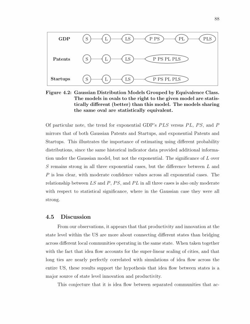
88
S L LS P PS PL PLS
S L LS P PS PL PLS
S L LS P PS PL PLSStartups
Patents
GDP
Figure 4.2: Gaussian Distribution Models Grouped by Equivalence Class.The models in ovals to the right to the given model are statis-tically different (better) than this model. The models sharingthe same oval are statistically equivalent.
Of particular note, the trend for exponential GDP’s PLS versus PL, PS, and P
mirrors that of both Gaussian Patents and Startups, and exponential Patents and
Startups. This illustrates the importance of estimating using different probability
distributions, since the same historical indicator data provided additional informa-
tion under the Gaussian model, but not the exponential. The significance of L over
S remains strong in all three exponential cases, but the difference between L and
P is less clear, with moderate confidence values across all exponential cases. The
relationship between LS and P , PS, and PL in all three cases is also only moderate
with respect to statistical significance, where in the Gaussian case they were all
strong.
4.5 Discussion
From our observations, it appears that that productivity and innovation at the
state level within the US are more about connecting different states than bridging
across different local communities operating in the same state. When taken together
with the fact that idea flow accounts for the super-linear scaling of cities, and that
long ties are nearly perfectly correlated with simulations of idea flow across the
entire US, these results support the hypothesis that idea flow between states is a
major source of state level innovation and productivity.
This conjecture that it is idea flow between separated communities that ac-

89
counts for state-level economic variations is supported by the significant increase in
model matches to data for GDP that are obtained when network structure is added
to population information. The fact that adding long ties to population model in-
creases the probability of the extended model fitness suggests that the correlation
between long ties and the GDP metric is due to a different phenomenon than that
associated with simple variation in population. Indeed, the Gowalla population is
mostly in hubs, as shown in Figure 4.1, so the structure rather than the locations
of users is responsible for the increase in matching. Furthermore this suggests the
flow of ideas happens largely between metropolitan areas.
In Granovetter’s work [56] which was cited earlier, the author discussed that
there are many criteria one can use to define strength of a tie. Even within com-
munity detection there are many decisions to be made, for example depending on
the algorithm, there may be room for overlapping communities, thresholds that can
be changed, or different methods of weighting ties. We find it telling that there
is a disparity in the fraction of long ties that are weak and the fraction of short
ties that are weak, and believe that this explains why long ties improved our eco-
nomic predictions more than short ties. It is a particularly attractive idea since it
encodes idea flow across borders, which a social network could contribute, but raw
population values would not.
It is also important to note that our subject sample were users of Gowalla,
both because users of Gowalla must have more than average disposable income in
order to be able to possess a smartphone and be innovative enough to embrace
technology that was at that time quite new and make use of such a location-based
social network. We believe that economic performance such as GDP or having
startups is furthered by the advancement and utilization of technology, and so the
Gowalla userbase may be a more appropriate sample than the U.S. population as a
whole. We do not, of course, believe that the Gowalla population is a representative
sample of the entire population, but rather a sample that is well suited to predicting
the economic factors we examined.

90
4.6 Summary
GDP, patents, and startups are three economic measurements that can be
used to quantify productivity and innovation. By modeling these measurements
using location-based social network data and embedding the ties into states, we
find that not only do we get a linear relationship with high correlation, but also
that the long tie network produces this correlation through different means than
the population-only model. While correlation is not causation, there is intuition
to support a conjecture that the long tie network features are connections that
allow diverse ideas to be shared among individuals. Since ideas may be readily
shared among individuals in a particular geographic region due to shared culture and
higher probability of regular interaction, long ties are an especially good candidate
for measuring the speed of sharing of novel ideas because they connect people acting
in separate innovation support infrastructures of different states.
Our results indicate that while we see improvements by combining long ties
and population for GDP prediction, we do not see the same behavior for predict-
ing patent or startups behavior. Patents are an unusual category in that they vary
wildly with respect to state population - one state may have a larger population and
much fewer patents, or the opposite may be true. The monetary benefit of innova-
tion related to patents is displayed in GDP, but the underlying workings of patent
development and application appears to not be strongly influenced by geographic
boundaries or ties. One plausible explanation why startups behave differently is
that only a small percentage of startups are innovation-based, while the majority
are self-employed individuals providing standard personal services.

CHAPTER 5
Influence of Knowledge of Friend of Friends on Social Search
5.1 Background
Social search has been well studied over the last 50 years. Briefly, the problem
involves tasking a person with utilizing social connections to attempt to reach a
target person. Milgram’s small-world work was notable for being an empirical social
experiment in which individuals used only connections with which they were on a
first-name basis to route a folder to a target person. We go into more details about
this experiment and related work in Section 2.3. We found the experiment to be
an interesting framework and applied it towards a similar task, an artificial social
search run on a network built from an actual social network which contained explicit
geographical information about its members.
Network scientists have recently calculated the distribution of the shortest
path lengths between randomly selected pairs of users in online social networking
sites and confirmed that the majority of people are on average within six degrees of
separation (e.g., 4.7 in Facebook [83], 3.7 in Myspace [84], 4.1 in Twitter [85], and so
on [86]). The online social network we selected, Gowalla, is built for location based
activities in which individuals ”check in” at physical locations. We found that the
social network of friendships cannot be described simply by the physical location
of users or co-location between them. This suggested that the network data [67]
was fairly diverse, which is a feature seen in real-world networks in contexts such
as economics [71], and more importantly in how actual users in a modern social
forwarding experiment select links [38].
A key feature in the success of small world experiments is that the networks
produce surprising short paths between random pairs of nodes in them. Networks
have been described with terms such as “small world” and “scale-free” [87], with
more formal definitions involving the average distance, diameter, or degree distribu-
tion parameter γ [88]. In these networks, either the number of edges must be very
high or else localized clusters must be connected by well-connected nodes with edges
91

92
that bridge gaps between otherwise distant groups of nodes. The idea of bridges,
and furthermore that they are in some capacity “weak ties” has been suggested in
literature [32], and is the basis for our social search. We do a more thorough exam-
ination of Granovetter’s work in Section 2.2. In the context of a social search there
are many ways we could consider weak ties, but we choose to specifically define weak
ties as cases where the friends of friends (FoFs) of a person are not also friends with
that same person.
To reflect the fact that a person is less likely to know much about a given
FoF, including whether or not the FoF is actually a friend of the mutual friend, we
consider a partial knowledge based on parameter κ ∈ [0.0, 1.0]. We describe how this
knowledge of FoF parameter is applied in more detail in Section 5.2. Our question
then is how is a social search based on rational protocols affected by changes to κ if
we allow decision making based on not just knowledge of friends, but FoF as well. As
a secondary topic, we explore the performance of several node selection criteria both
as an independent basis for social routing protocols and in combinations with other
criteria as hybrid protocols. We find that the criteria used, the order of precedence of
criteria, and κ all have a meaningful impact on the behavior of social search. While
we cannot directly establish what the underlying mechanisms are, we can conclude
that having FoF knowledge as well as the particular types of information we have
about our contacts both play a significant part in people being able to perform an
effective social search.
5.2 Methods
As previously mentioned in Section 5.1, our social network came from ex-
isting work which included collecting data on the location-based social network
Gowalla [67], the same data that was used in Chapter 4. This was a global net-
work with populations primarily in the United States and Sweden, and it contained
154,557 nodes and 1,139,110 edges with γ ≈ 1.51. We refer to the entire network as
“Global”, and the network containing only nodes in the United States as “US-Only”.
US-Only contained 75,803 nodes and 454,350 edges with γ ≈ 1.49. The Global net-
work was connected, meaning the giant component of both networks contained all

93
the nodes in the network. The US-Only network was very close to being connected,
with the giant component containing 75,690 nodes and 454,284 edges. Since the
giant component encompassed almost all of the network and by definition a path
existed between any two nodes in it, we made use of only this component for our
studies on US-Only. We also constructed a “Filtered” network from the US-Only
network by removing any nodes that failed to satisfy at least one of two criteria:
1) Being within 100km of each other or 2) Having checked in at the same location
(latitude and longitude) within 15 minutes of each other. Filtered had several small
components and just one sizable giant component, so we focused only on the giant
component which contained 55,786 nodes and 196,882 edges with γ ≈ 1.85. The
justification for the Filtered distance restriction was that 100km encompasses the
size of even larger metropolitan areas such as Los Angeles, so anything outside of
this range was unlikely to be a local friend since friends are mainly located at short
distances from each other [68].
In each case of our emulation, we selected a source and target node from the
network, and then ran a social search for up to 50 hops. We required that the
source and target be at least 500 mi (804 km) apart so that trivial searches were
not performed. This distance limitation was in line with the spirit of Milgram’s
experiment, but we chose to constrain our search based on the north-south distance
of the U.S. since we were selecting random pairs. In each hop, the current node
would select one node to forward the imaginary packet to, with the stipulation that
no node previously visited in the search could be used again. If the target received
the packet, the search stopped.
The biggest design decision in our social search experiment was deciding how
a node would select the next node in the forwarding chain (we preserve here the
original language of Milgram experiment, in graph theory language we chose the
next node on a path.) To this end, we designed several protocols that seemed
consistent with how a rational agent might make a decision, as well as a baseline
random protocol. Each of the protocols can be viewed as a filter on the friends and
FoF of a given node. At each step, the node first checks if the target is a friend
or friend of friend. If it is friends with the target, the packet is forwarded directly

94
to the target so that the chain is completed. If the target is not a friend, but is
a FoF, then the packet is forwarded to one of the mutual friends. If neither of
these conditions is true, the node applies any filters (via protocols) that are allowed,
and then decides based on the “best” choice remaining. If there is a tie in criteria
between friends and FoFs, the next recipient is selected from friends. If there is a
tie internally within friends or within FoFs, it is resolved randomly.
Each of these single-criterion protocols was denoted by a single letter which
represented the criterion used in it:
• Random, R (zero criteria): If the current node has a friend that is the target
it routes directly to the target. Otherwise if it has a FoF that is the target,
it routes to the corresponding friend. If neither condition is met, the current
node picks a friend at random.
• Distance, D: The current node considers the distance from each of its friends
and FoFs to the target. Since details about exact addresses are less frequently
known, we consider movement between two nodes within 50km of the target
and to a node that is less than 25% closer to the target than the current node
to be “distance equivalent,” meaning that such a move does not improve the
distance to target aspect of the search. The 50km radius covers about 45%
of friends for the average node, based on US-only’s friendship densities which
are shown in Table 5.1. If the target is not in the current node’s list of friends
or FoFs, the node considers the minimum distances from nodes that are not
“distant equivalent” class, as only movement to nodes not belonging to the
class improves the search with respect to distance. If all possible nodes are
within the class, then in this single criterion strategy, the node will select
randomly from among the “distance equivalent” nodes. As mentioned before,
preference is given to friends over FoFs if there are “best” choices within both
sets. The value of the distance equivalent class is higher for multi-criteria
search, which we discuss later in the chapter.
• Popularity, P: The current node considers all friends and FoF with a score
of dlog2(degree)e, where degree is the friend or FoF’s degree. Our reasoning

95
is that it is difficult to judge the difference in impact on the social search
that choosing a friend with 10 friends versus 15 friends will have, so they are
considered to be “popularity equivalent,” meaning that choosing one over that
other cannot be based on popularity alone. It is however easier to rationalize
that there will likely be a positive impact in choosing a node with 200 friends as
opposed to one with 100 friends. While we did find a small degree of sensitivity
to the scoring function in our results, it wasn’t enough to change the general
behavior of the social search or affect any of our findings. Modeling a score that
mirrors how an actual human would differentiate between degrees of nodes is
both outside the scope of our work and not a goal of our social search task
since we make no claim that this is how a real human would act. Instead we
simply aim to have a justifiable protocol based on criteria easily accessible to
a theoretical agent, and we believe the proposed log scoring achieves this goal.
The behavior when the target is within a hop from a friend of FoF is unchanged
from the other cases; forwarding will happen without consideration of score.
Otherwise, a node with the maximum score is selected as the next recipient.
Preference is given to friends selected for their own score over friends selected
because of a connection to a particular FoF, and ties are resolved through
random selection.
• Community, C: The current node considers whether or not any its friends and
FoFs is in the same community as the target. If the target is not within the
node’s friends or FoFs, the current node forwards to a friend in the target’s
community, resolving ties randomly and preferring friends who are directly in
the target community over friends who are merely connected to FoFs in the
target community. If there is no candidate in the target community, the node
selects randomly from among its friends.
In this context, community refers to clustering the social network into similar
groups (communities). We chose to do this through GANXiS [76], and used
the overlapping community results with r = 0.5 on the Global data set. We
did not detect communities again for the US-Only case, and simply ignored

96
any nodes that were not part of the US-Only network. Since the Filtered
data set was markedly different, we ran GANXiS separately on this data to
generate a new set of communities. Due to the nature of Filtered, we chose to
require that all communities proposed have a size of at least 5 nodes. However
it is difficult to have ground truth in community detection, especially when
the context of communities is unclear, so we do not claim that these were
the “best” community sets but maintain that they were representative sets to
use derived from a state-of-the-art system. Our protocol design would remain
the same for any arrangement for detecting communities. The information
that is available about any node’s community membership is simply which
community IDs they have; in our work communities do not overlap so each
node is mapped to exactly one community ID.
Table 5.1: Friendship Density by Distance Range, US-Only. The averagedensity of friends at each distance range, computed by takingthe density in each range for each individual node’s immediateneighborhood (friends), and then averaging the densities. Thisis instead of computing densities based on the number of nodesin the entire network.
Distance Range (km) % of Friends Cumulative %≤6.25 18.6 18.6
6.25 – 12.50 8.6 27.212.50 – 25.00 10.3 37.625.00 – 50.00 7.6 45.250.00 – 100.00 3.9 49.0100.00 – 200.00 3.8 52.8200.00 – 400.00 6.4 59.2400.00 – 800.00 6.4 65.6800.00 – 1600.00 11.8 77.41600.00 – 3200.00 14.8 92.23200.00 – 6400.00 7.5 99.8
We also designed several hybrid protocols which used multiple criteria with
the same notation as in the single protocol case. If there was a tie (same distance,
no node in the target community, etc.) in the criterion denoted by the first letter
(reading left to right), then the hybrid protocol would use the next criterion. In cases

97
with more than two criteria, the protocol could keep deferring to the next criterion
if necessary. If there was still a tie between candidates once a hybrid protocol
had no more criteria remaining, it would simply pick randomly from among those
candidates.
As an example, DC would first try to find a forwarding node based on whether
or not it was the target, and if that failed it would then try to minimize the distance
to the target. If D would have resorted to random selection, then the current node
would instead consider those candidates based on whether or not they had mem-
bership in the target node’s community instead of defaulting to picking randomly.
If a subset (possibly the entire set) of candidates was in the target community, the
current node would be forced to pick randomly from among them. Defaulting back
to random happens in all hybrid protocols because even if one protocol falls short in
producing candidates, the combination of protocols carries more information than
a single protocol would and it is much more likely that a node further along even
a short chain will be able to use some of these criteria to make a better informed
decision.
The other important aspect is how knowledge about friends of friends (κ ∈[0, 1]) was applied. At the beginning of the social search, every pair of friends (h, i)
was mapped to a list of all nodes that were friends of i but were not h. Every
entry in the sublists then had a random number drawn from a uniform distribution
between 0 and 1 assigned to it. When considering a pair of nodes h and j with
edges (h, i) and (i, j) in the social network, j was only a FoF of h if the random
value for j in the list mapped to (h, i) was ≤ κ. In this way, we did not alter the
actual network structure, but instead altered the effective perception of each node.
We considered the four single criterion protocols, all six hybrids comprised of
two criteria, and all six hybrids comprised of D, C, and P . For each data set and
protocol, we ran 100 trials with a maximum chain length of 50 hops. For each case
we evaluated these at κ = 0.0, 0.2, 0.8, 1.0. For the US-Only data set we also ran
our social search with κ = 0.05, 0.10, 0.15. In all experiments we used the same seed
for determining the FoF knowledge numbers, and across protocols using the same
data set we selected the same starting and target nodes. The random seed was then

98
reset to a different value after generating FoF numbers in each simulation so the
traversed paths were non-deterministic.
5.3 Results
From our social searches, we were able to collect general results such as an
estimate of how successful our protocols would be on the data sets tested, and how
often knowledge of friends of friends was leveraged (Tables 5.2-5.4). The immediately
apparent trends are that in most cases κ = 0.0 yields low success rates (i.e. only a
small number of chains reach the target), that success rate and the number of chains
that utilize FoF knowledge generally increases as κ increases, and that the average
hop length tends to decrease as κ increases. C-first methods not follow the κ = 0.0
trend, and we discuss why this is in Section 5.4.
In addition to the tabulated results, we also were able to examine the distribu-
tion of chain lengths among successful social searches. This allowed us to compare
the same protocol across different data sets by examining the shape of the distribu-
tion on a case-by-case basis for each κ as well. However, we do not provide every
distribution as this would be highly redundant without giving additional insight.
In Figures 5.1–5.2 we compare DP in Filtered and US-Only. It is important to
examine what the number of successful chains (paths that made it from the starting
node to the target node), Ns, is in each case since the curves are normalized to Ns
to make comparisons more fair. By doing so, the value of interpreting the κ = 0.2
curve is decreased since NUS−Onlys = 61, but NFiltered
s = 13. Even for κ > 0.2,
NFiltereds ≈ 20 while NUS−Only
s ≥ 80, so the curves in Figure 5.2 are noisier than
those in Figure 5.1. Regardless of the noise, the difference in peaks between US-
Only and Filtered is clear, as is the consistent peak position between κ = 0.8 and
κ = 1.0 in the US-Only case. The overlapping peaks do not occur in the Filtered
case, indeed the less connected network results in even the successful chains with
κ = 0.8 to have hop lengths almost evenly distributed between 2 and 12.
Another indication that the strategy guiding the creation of the Filtered net-
work (i.e. eliminating distant low-interacting friends as viable choice for routing) is
not successful or well-suited for our study is in the success rates for R in Filtered

99
Table 5.2: Social Search Results on Global. Ns is the number of successfulchains (path reached target) out of 100, Hs is the averagenumber of hops (chain length) in successful chains, and FoFs isthe number of successful chains where at least one node madea forwarding decision that was influenced by knowledge abouttheir FoFs. We omit FoFs for κ = 0.0 since it is always 0 bydesign. The numerical values in bold font are the best in theircolumns, and bold blue protocols correspond to rows with fiveor more bold values. Protocols are described in Section 5.2.
κ = 0.0 κ = 0.2 κ = 0.8 κ = 1.0Protocol Ns Hs Ns Hs FoFs Ns Hs FoFs Ns Hs FoFsR 3 17.67 35 13.71 33 53 15.85 53 56 13.41 56D 17 20.00 44 14.84 43 64 11.55 64 66 11.24 66P 33 10.70 69 7.86 61 90 5.27 90 93 5.66 93C 16 16.44 57 11.28 53 61 9.56 60 62 9.79 61DP 16 18.69 69 8.48 66 89 6.19 89 92 6.18 92DC 2 3.00 39 5.82 39 53 4.68 53 53 4.34 53CD 14 8.21 69 8.83 65 83 6.63 72 87 6.10 79CP 74 10.78 87 8.32 72 96 6.30 83 97 6.84 84PD 10 3.20 72 8.13 68 92 6.18 92 94 5.77 94PC 10 3.20 47 6.87 43 71 4.80 71 74 4.78 74DPC 8 11.63 58 5.83 51 73 4.74 59 74 4.65 59DCP 2 3.00 53 6.28 53 62 5.63 62 63 4.81 62PDC 10 3.20 63 6.95 58 82 4.67 76 85 4.59 78PCD 10 3.20 51 6.69 43 71 4.30 64 72 4.13 65CDP 12 7.75 74 7.28 66 87 6.05 72 91 5.85 77CPD 18 3.78 84 7.14 71 95 6.23 81 98 6.59 83
and US-Only. The protocol’s random routing, even with increasing κ, yields almost
no successful searches in Filtered, while US-Only gets a moderate success rate of
up to 61% by κ = 1.0. If the structure was similar we would expect that since the
number of nodes is far less in Filtered, the diameter of the network should decrease
and random routing would have equal or better chances of succeeding within the
50 hop limit. Furthermore, literature proves that in the real world the small world
effect is measurable in social search tasks, and the Gowalla social network is a real
subset of the full real-world contact network. However, we still consider the behavior
of our artificial social search run on Filtered and compare the results in depth with
those from running on US-Only in Section 5.4.
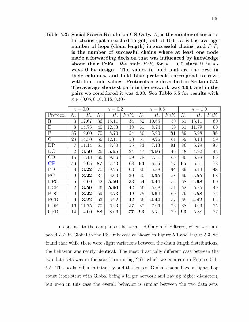
100
Table 5.3: Social Search Results on US-Only. Ns is the number of success-ful chains (path reached target) out of 100, Hs is the averagenumber of hops (chain length) in successful chains, and FoFsis the number of successful chains where at least one nodemade a forwarding decision that was influenced by knowledgeabout their FoFs. We omit FoFs for κ = 0.0 since it is al-ways 0 by design. The values in bold font are the best intheir columns, and bold blue protocols correspond to rowswith four bold values. Protocols are described in Section 5.2.The average shortest path in the network was 3.94, and in thepairs we considered it was 4.03. See Table 5.5 for results withκ ∈ {0.05, 0.10, 0.15, 0.30}.
κ = 0.0 κ = 0.2 κ = 0.8 κ = 1.0Protocol Ns Hs Ns Hs FoFs Ns Hs FoFs Ns Hs FoFsR 3 12.67 36 15.11 34 52 10.65 50 61 13.11 60D 8 14.75 40 12.53 38 61 8.74 59 61 11.79 60P 35 9.60 70 8.70 54 86 5.90 81 89 5.98 88C 28 14.50 56 12.11 53 61 9.26 61 59 8.14 59DP 7 11.14 61 8.30 55 83 7.13 81 86 6.29 85DC 2 3.50 26 5.65 24 47 4.66 46 48 4.92 48CD 15 13.13 66 9.86 59 78 7.81 66 80 6.98 66CP 76 9.05 87 7.43 68 93 6.55 77 95 5.51 78PD 9 3.22 70 9.26 63 86 5.88 84 89 5.44 88PC 9 3.22 37 6.00 30 60 4.35 58 69 4.55 68DPC 5 6.60 42 5.50 33 64 4.44 55 68 4.68 60DCP 2 3.50 46 5.96 42 56 5.68 51 52 5.25 49PDC 9 3.22 59 6.73 49 75 4.64 69 79 4.58 75PCD 9 3.22 53 6.92 42 66 4.44 57 69 4.42 64CDP 16 11.75 70 6.93 57 87 7.06 73 88 6.63 75CPD 14 4.00 88 8.66 77 93 5.71 79 93 5.38 77
In contrast to the comparison between US-Only and Filtered, when we com-
pared DP in Global to the US-Only case as shown in Figure 5.1 and Figure 5.3, we
found that while there were slight variations between the chain length distributions,
the behavior was nearly identical. The most drastically different case between the
two data sets was in the search run using CD, which we compare in Figures 5.4–
5.5. The peaks differ in intensity and the longest Global chains have a higher hop
count (consistent with Global being a larger network and having higher diameter),
but even in this case the overall behavior is similar between the two data sets.
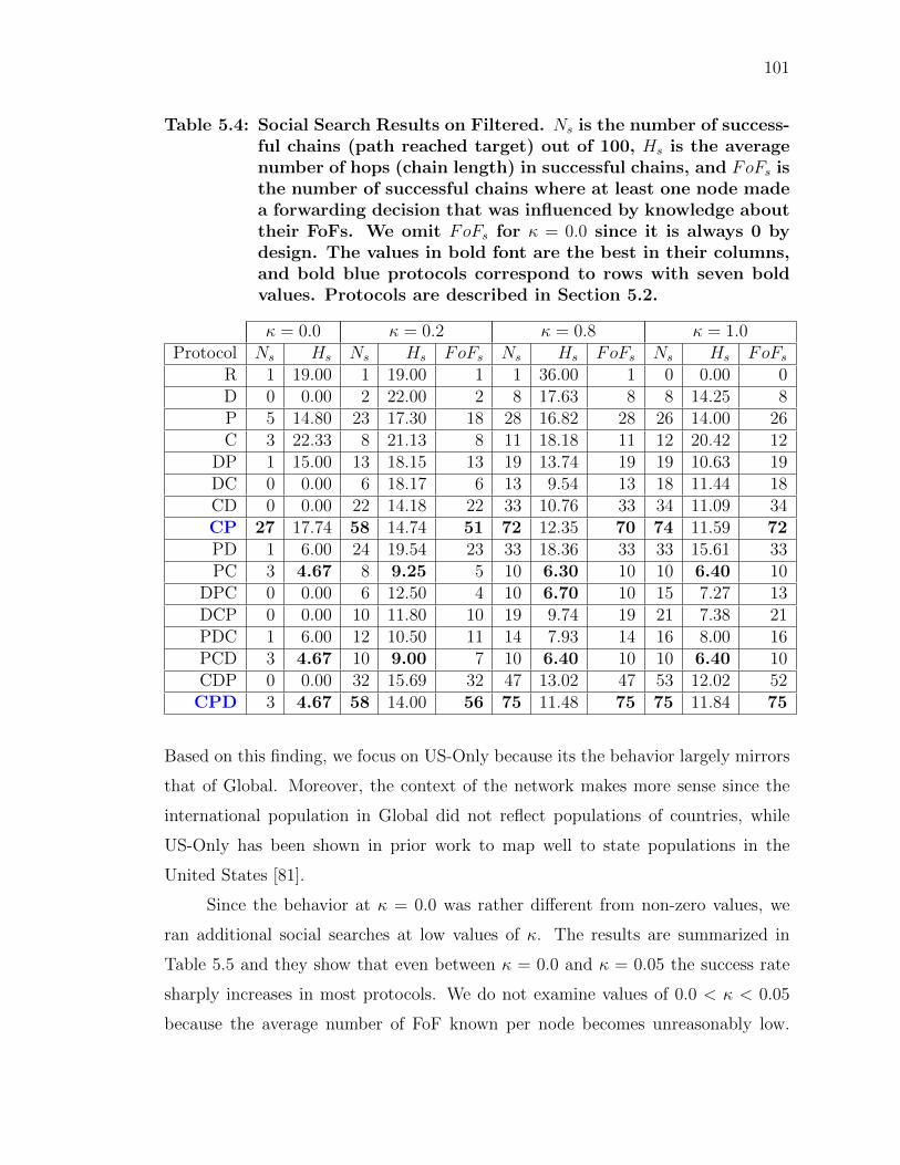
101
Table 5.4: Social Search Results on Filtered. Ns is the number of success-ful chains (path reached target) out of 100, Hs is the averagenumber of hops (chain length) in successful chains, and FoFs isthe number of successful chains where at least one node madea forwarding decision that was influenced by knowledge abouttheir FoFs. We omit FoFs for κ = 0.0 since it is always 0 bydesign. The values in bold font are the best in their columns,and bold blue protocols correspond to rows with seven boldvalues. Protocols are described in Section 5.2.
κ = 0.0 κ = 0.2 κ = 0.8 κ = 1.0Protocol Ns Hs Ns Hs FoFs Ns Hs FoFs Ns Hs FoFs
R 1 19.00 1 19.00 1 1 36.00 1 0 0.00 0D 0 0.00 2 22.00 2 8 17.63 8 8 14.25 8P 5 14.80 23 17.30 18 28 16.82 28 26 14.00 26C 3 22.33 8 21.13 8 11 18.18 11 12 20.42 12
DP 1 15.00 13 18.15 13 19 13.74 19 19 10.63 19DC 0 0.00 6 18.17 6 13 9.54 13 18 11.44 18CD 0 0.00 22 14.18 22 33 10.76 33 34 11.09 34CP 27 17.74 58 14.74 51 72 12.35 70 74 11.59 72PD 1 6.00 24 19.54 23 33 18.36 33 33 15.61 33PC 3 4.67 8 9.25 5 10 6.30 10 10 6.40 10
DPC 0 0.00 6 12.50 4 10 6.70 10 15 7.27 13DCP 0 0.00 10 11.80 10 19 9.74 19 21 7.38 21PDC 1 6.00 12 10.50 11 14 7.93 14 16 8.00 16PCD 3 4.67 10 9.00 7 10 6.40 10 10 6.40 10CDP 0 0.00 32 15.69 32 47 13.02 47 53 12.02 52
CPD 3 4.67 58 14.00 56 75 11.48 75 75 11.84 75
Based on this finding, we focus on US-Only because its the behavior largely mirrors
that of Global. Moreover, the context of the network makes more sense since the
international population in Global did not reflect populations of countries, while
US-Only has been shown in prior work to map well to state populations in the
United States [81].
Since the behavior at κ = 0.0 was rather different from non-zero values, we
ran additional social searches at low values of κ. The results are summarized in
Table 5.5 and they show that even between κ = 0.0 and κ = 0.05 the success rate
sharply increases in most protocols. We do not examine values of 0.0 < κ < 0.05
because the average number of FoF known per node becomes unreasonably low.

102
0
0.05
0.1
0.15
0.2
0.25
0.3
0.35
0 5 10 15 20 25
Fra
ctio
n o
f A
ll S
ucce
sse
s
Chain Length
k=0.2k=0.8k=1.0
Figure 5.1: Successful DP Chain Lengths in US-Only. A comparison ofchain length distributions among successful chains using theDP protocol run on the US-Only data set. κ = 0.0 is omitteddue to an insufficient number of chains completing.
Instead this result suggests that even a modest amount of knowledge about one’s
FoFs can result in a significant increase in social search efficiency.
While increasing κ in general increases Ns, not every path that was successful
at a particular value of κ remained successful at a higher value of κ. Table 5.6
shows how often this adverse effect of higher knowledge occurred for every pair of
closest κ values. The results for R are not particularly significant since the protocol
acts randomly. Protocols utilizing a single criterion were most susceptible to the
adverse effect, though CD was also notably sensitive. Conversely, P was relatively
unaffected, suggesting that more information about links can be beneficial but rarely
is detrimental in path selection.
Protocols utilizing D experience the largest incidence of the effect. Protocols
with a first criterion of communities (i.e. starting with C) also exhibited more paths

103
0
0.05
0.1
0.15
0.2
0.25
0.3
0.35
0 5 10 15 20 25
Fra
ctio
n o
f A
ll S
ucce
sse
s
Chain Length
k=0.2k=0.8k=1.0
Figure 5.2: Successful DP Chain Lengths in Filtered. A comparison ofchain length distributions among successful chains using theDP protocol run on the Filtered data set. κ = 0.0 is omitteddue to an insufficient number of chains completing. κ = 0.2has around 10 successful chains in Filtered but is includedfor consistency.
that failed at a higher κ. When P was the leading part of a protocol the paths that
succeeded very rarely failed at a higher κ. As shown in Table 5.3, these protocols
had high success rates in general, with P having a moderate success rate even at
κ = 0.0, so the lack of paths falling victim to the adverse effect was not due to a
lack of successful paths.
Another question we wanted to address was how similar were paths with no
FoF knowledge (i.e. κ = 0.0) to paths that had access to FoF knowledge and
used it in making forwarding decisions. The number of paths matching across all
values of κ (All) and matching between κ = 0.0 and at least one other value of κ
(One+) are in Figure 5.6. Interestingly, some protocols had many matching paths

104
0
0.05
0.1
0.15
0.2
0.25
0.3
0.35
0 5 10 15 20 25 30
Fra
ctio
n o
f A
ll S
ucce
sse
s
Chain Length
k=0.2k=0.8k=1.0
Figure 5.3: Successful DP Chain Lengths in Global. A comparison ofchain length distributions among successful chains using theDP protocol run on the Global data set. κ = 0.0 is omitteddue to an insufficient number of chains completing.
for One+, and PC had about 30% of paths matching across all knowledge levels.
Protocols involving P and C together exhibited the most matching, particularly
across all knowledge levels. This suggests that the search space is most constrained
by considering community membership and popularity of friends, with the order in
which criteria are applied mattering greatly.
5.4 Discussion
While our social search was inspired by the small world experiments of Mil-
gram, our goal was not to perform another social experiment nor was it to produce
results that were close to existing small world experiments. Instead, using social
network data, we wanted to examine the impact of empirically observed data on a

105
0
0.05
0.1
0.15
0.2
0.25
0.3
0.35
0 5 10 15 20 25 30
Fra
ctio
n o
f A
ll S
ucce
sse
s
Chain Length
k=0.2k=0.8k=1.0
Figure 5.4: Successful CD Chain Lengths in US-Only. A comparison ofchain length distributions among successful chains using theCD protocol run on the US-Only data set. κ = 0.0 is omitteddue to an insufficient number of chains completing.
synthetic social search and see the effects of knowledge of FoFs, as well as the im-
portance of different criteria for selecting intermediate nodes. However, it is worth
remarking that our data sets represented a smaller network than the 1960s United
States contact network, and that while Gowalla users are likely to be more efficient
searchers than a random individual one can imagine that with a few extra hops to
randomly enter and leave the Gowalla network, a right-shifted chain length distri-
bution similar to ours might be produced in an real-world experiment. In this case,
several protocols would yield a curve similar in position and shape to Milgram’s
experiments, including two peaks and an average hop length of around 5-7. Fig-
ures 5.4–5.5 are two examples that demonstrate the similarities between our artificial
search and Milgram’s results in [34].
The degree to which our emulated social search succeeds is drastically affected

106
0
0.05
0.1
0.15
0.2
0.25
0.3
0.35
0 5 10 15 20 25 30
Fra
ctio
n o
f A
ll S
ucce
sse
s
Chain Length
k=0.2k=0.8k=1.0
Figure 5.5: Successful CD Chain Lengths in Global. A comparison ofchain length distributions among successful chains using theCD protocol run on the Global data set. κ = 0.0 is omitteddue to an insufficient number of chains completing.
by the protocol chosen, ranging from less successful (e.g. R or DCP ) to nearly
always successful in several cases. In addition to what criteria the agents use to
select what they believe to be the most suitable node, the amount of knowledge they
have about FoFs has a large impact on the success rate. Generally, as κ increases,
the success rate increases. This may be due to the diversity of forwarding options
two hops away increasing, which while occasionally detrimental to the search by
going down a false path, more often than not reveals a more suitable node that can
decrease the chain length or turn an otherwise unsuccessful chain into a completed
one. Since we did not allow backtracking (as mentioned in Section 5.2) making the
wrong forwarding choice could lead to a search terminating unsuccessfully, and more
information about the 2-hop neighborhood decreases the chances of a node making
a dead-end choice.

107
Table 5.5: Additional Social Search Results on US-Only For Lower Valuesof κ. Ns is the number of successful chains (out of 100), Hs isthe average number of hops (chain length) in successful chains,and FoFs is the number of successful chains where at leastone node made a forwarding decision that was influenced byknowledge about their FoFs. We omit FoFs for κ = 0.0 sinceit is always 0 by design. The values in bold font are the bestin their columns, and bold blue protocols correspond to rowswith six bold values. Protocols are described in Section 5.2.
κ = 0.05 κ = 0.10 κ = 0.15Protocol Ns Hs FoFs Ns Hs FoFs Ns Hs FoFsR 27 14.31 20 29 16.07 24 29 17.26 23D 26 13.69 23 39 15.13 37 41 9.93 38P 54 9.74 32 61 9.69 42 63 8.92 44C 53 15.06 36 51 11.69 44 48 10.92 38DP 43 13.23 37 57 12.19 52 55 8.93 50DC 14 5.29 12 20 5.85 18 21 7.24 20CD 62 11.74 55 67 10.54 58 62 8.18 54CP 79 8.66 52 85 8.33 58 88 7.51 67PD 58 11.74 50 62 10.13 54 64 9.78 56PC 25 6.92 18 28 6.00 21 30 4.43 22DPC 32 8.81 25 38 7.58 32 40 7.43 33DCP 30 5.53 27 42 5.26 38 40 5.60 37PDC 47 7.45 37 51 7.65 42 53 7.49 43PCD 38 7.55 23 43 6.51 29 46 7.63 33CDP 66 8.05 53 73 8.00 61 69 7.55 58CPD 84 9.24 73 85 8.04 75 85 7.82 74
From comparing Filtered to the networks from our other data sets, either by
the chain length distributions discussed in Section 5.3 or by examining the net-
work structure more directly, it is clear that by restricting the friendship network
to geographic relationships (co-location at a particular time or a bound on physical
distance between reported home locations) we lose a critical portion of the network.
In Figures 5.7–5.9 we show the degree distributions of the three data sets and in Fig-
ures 5.10–5.12 we show the complementary cumulative degree distribution (CCDF)
for each data set.
In these plots, Global and US-Only have slight differences between each other
but are very similar in overall structure, containing fat tails and very similar power

108
Table 5.6: Adverse Effects of Increasing κ on US-Only. Each cell showshow many times a social search executed from a given sourceto target succeeded at the lower κ1 but failed at higher κ2 whenusing a particular protocol, with the percentage of Ns at κ1 inparentheses. Column headings are in the form of “κ1, κ2.”
Protocol 0.00, 0.05 0.05, 0.10 0.10, 0.15 0.15, 0.20 0.20, 0.80 0.80, 1.0CP 4 (5.3) 2 (2.5) 2 (2.4) 3 (3.4) 1 (1.1) 0 (0.0)DCP 0 (0.0) 1 (3.3) 4 (9.5) 5 (12.5) 7 (15.2) 4 (7.1)DP 0 (0.0) 0 (0.0) 6 (10.5) 5 (9.1) 0 (0.0) 0 (0.0)CD 2 (13.3) 9 (14.5) 12 (17.9) 8 (12.9) 6 (9.1) 6 (7.7)D 4 (50.0) 8 (30.8) 7 (17.9) 12 (29.3) 6 (15.0) 14 (23.0)C 6 (21.4) 19 (35.8) 16 (31.4) 12 (25.0) 14 (25.0) 16 (26.2)R 0 (0.0) 9 (33.3) 11 (37.9) 9 (31.0) 4 (11.1) 10 (19.2)P 0 (0.0) 0 (0.0) 2 (3.3) 0 (0.0) 1 (1.4) 1 (1.2)PD 0 (0.0) 1 (1.7) 0 (0.0) 1 (1.6) 0 (0.0) 0 (0.0)PC 0 (0.0) 1 (4.0) 0 (0.0) 0 (0.0) 0 (0.0) 0 (0.0)DC 1 (50.0) 2 (14.3) 5 (25.0) 6 (28.6) 4 (15.4) 6 (12.8)DPC 0 (0.0) 3 (9.4) 1 (2.6) 5 (12.5) 5 (11.9) 0 (0.0)PDC 0 (0.0) 0 (0.0) 0 (0.0) 0 (0.0) 0 (0.0) 0 (0.0)PCD 0 (0.0) 0 (0.0) 0 (0.0) 0 (0.0) 0 (0.0) 0 (0.0)CDP 1 (6.3) 4 (6.1) 6 (8.2) 3 (4.3) 2 (2.9) 0 (0.0)CPD 0 (0.0) 3 (3.6) 2 (2.4) 1 (1.2) 3 (3.4) 0 (0.0)
law parameters of γ ≈ 1.5. In contrast, the Filtered network has γ = 1.85 but
behaves less like an ultra small-world network [88] and should not be considered one
since the CCDF in Figure 5.12 lacks the characteristic power law decay in the tail of
the distribution. Furthermore, the claim that Global and US-Only are small world
networks is supported by the fact that while the diameter of the Global network is 14
and 11 for the US-Only network, the chain lengths observed are often significantly
shorter than the diameter. Based on the contextual difference between Filtered and
the other two data sets, we propose that the social network which is built on more
than just observed geographical features is essential to effective social searches. We
can consider the edges in Filtered to represent strong ties since friends are much
more likely to be within close proximity to each other [68], and the other edges in
Global and US-Only as weak ties which as discussed in Section 5.1 are necessary to
bridge gaps between otherwise distant clusters of nodes.
We further compare the US-Only and Filtered data sets by looking at their

109
0
10
20
30
40
50
60
70
80
DP D R CD CDP C PD DPC CPD P DCP DC CP PC PDC PCD
Pa
ths M
atc
he
d
All
One+
Figure 5.6: Path Consistency in US-Only. A comparison of consistencyin paths across various protocols for US-Only. Each pointin the “All” series represents how many source-target pairsused the same path across all seven knowledge levels. Inthe “One+” series, each point represents how many source-target pairs had at least one κ > 0.0 that matches the paththat κ = 0.0 used.
FoF distributions in Figures 5.13–5.14, the density of communities by distance in Ta-
bles 5.8–5.9, the sizes of communities in Figures 5.15–5.16, and the Filtered friend-
ship densities by distance in Table 5.7. The friendship densities by distance for
US-Only were shown earlier in Table 5.1. It is clear that almost all the friendships
in the Filtered network exist within 50–100km of each other, which is natural given
the way Filtered was generated. While only 28.5% of communities were within 50km
of nodes in the US-Only data set, the same distance threshold accounted for 71.6%
of communities in Filtered. The group of friends of friends for the average node
in US-Only is larger than that for a node in Filtered. From looking at the FoF
distributions it is evident that not only are there many more high frequency points
for sizes larger than e6, but that there are more nodes in Filtered with very small
totals of friends of friends, despite Filtered having significantly fewer nodes overall.
These observations further our assertion that US-Only and Filtered are significantly
different in network structure, and subsequently in geographical structure.

110
e2
e4
e6
e8
e10
e12
e1
e2
e3
e4
e5
e6
Fre
quency
Degree
Figure 5.7: Gowalla Degree Distribution, Global. Degree distributionsfor the Global data set, on log-log scales. The fat-tailed be-havior characteristic of small world/scale-free networks is ap-parent.
e2
e4
e6
e8
e10
e12
e1
e2
e3
e4
e5
e6
e7
Fre
quency
Degree
Figure 5.8: Gowalla Degree Distribution, US-Only. Degree distributionsfor the US-Only data set, on log-log scales. The fat-tailedbehavior characteristic of small world/scale-free networks isapparent.

111
e2
e4
e6
e8
e10
e12
e1
e2
e3
e4
e5
e6
e7
Fre
quency
Degree
Figure 5.9: Gowalla Degree Distribution, Filtered. Degree distributionsfor the Filtered data set, on log-log scales. The thinning outof higher degree nodes can be seen, making this distributionrather different from Global or US-Only.
e-12
e-10
e-8
e-6
e-4
e-2
e0
e0
e1
e2
e3
e4
e5
e6
e7
e8
e9
e10
P(k
)
k
Figure 5.10: Gowalla Global Complementary Cumulative DistributionFunction (CCDF). Following popular notation we use k todenote degree. Plots are on a log-log scale.

112
e-12
e-10
e-8
e-6
e-4
e-2
e0
e1
e2
e3
e4
e5
e6
e7
e8
e9
P(k
)
k
Figure 5.11: Gowalla US-Only Complementary Cumulative DistributionFunction (CCDF). Following popular notation we use k todenote degree. Plots are on a log-log scale.
To illustrate our case more clearly, in Figure 5.17 we show the Gowalla user
hubs based on the US-Only data set (a superset of the Filtered data set), and in
Table 5.10 we compare the fraction of the Gowalla users that these hubs accounted
for to the proportion of the actual US population living in these metropolitan areas.
Particularly in California and Texas, the US-Only data contains a larger propor-
tion of the Gowalla users than the fraction of the US population living there, with
US-Only having nearly double the total proportion of Gowalla users in metros com-
pared to their population. Since interactions are much more likely when local due
to both heightened chances of lower effort meetings and tendency of humans not
to travel far [89], it follows that the Filtered network is much more concentrated
in metropolitan areas than US-Only, which our examination of friendship and com-
munity densities corroborates as well. It is not surprising that D based approaches
are far less effective in Filtered given all of the differences in structure we have dis-
cussed. To show that the start and target distribution is reasonable, we compare the
actual start locations (Figure 5.18) and actual target locations (Figure 5.19) with
randomly selected starting locations (Figure 5.20) and randomly selected target
locations (Figure 5.21).
Despite the differences between the two networks, the sizes of communities
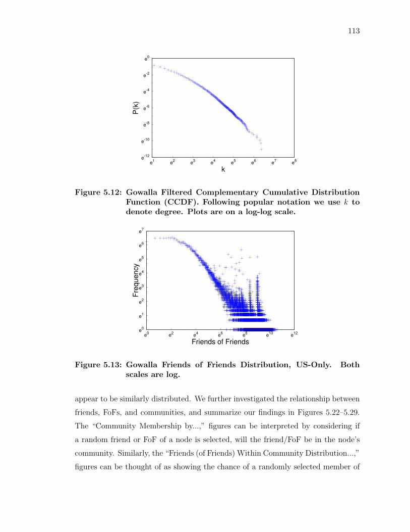
113
e-12
e-10
e-8
e-6
e-4
e-2
e0
e1
e2
e3
e4
e5
e6
e7
e8
P(k
)
k
Figure 5.12: Gowalla Filtered Complementary Cumulative DistributionFunction (CCDF). Following popular notation we use k todenote degree. Plots are on a log-log scale.
e0
e1
e2
e3
e4
e5
e6
e7
e0
e2
e4
e6
e8
e10
e12
Fre
quency
Friends of Friends
Figure 5.13: Gowalla Friends of Friends Distribution, US-Only. Bothscales are log.
appear to be similarly distributed. We further investigated the relationship between
friends, FoFs, and communities, and summarize our findings in Figures 5.22–5.29.
The “Community Membership by...,” figures can be interpreted by considering if
a random friend or FoF of a node is selected, will the friend/FoF be in the node’s
community. Similarly, the “Friends (of Friends) Within Community Distribution...,”
figures can be thought of as showing the chance of a randomly selected member of

114
e0
e1
e2
e3
e4
e5
e6
e7
e8
e0
e1
e2
e3
e4
e5
e6
e7
e8
e9
Fre
quency
Friends of Friends
Figure 5.14: Gowalla Friends of Friends Distribution, Filtered. Bothscales are log.
e0
e1
e2
e3
e4
e5
e6
e7
e0
e1
e2
e3
e4
e5
e6
e7
e8
Fre
quency
Fraction
Figure 5.15: Community Sizes, US-Only
the node’s community being a friend or FoF of the node. As already shown in Fig-
ures 5.15–5.16, the community sizes do not line up with the degree distribution, so
many communities will have more members than its constituent nodes have friends.
While a large portion of US-Only nodes have all their friends within their commu-
nity, only a small fraction of friends-of-friends are present in communities typically.
Due to the more compact nature of Filtered, both friends and FoFs are typically
represented in communities, shown explicitly in Figure 5.26 and Figure 5.27.
In both data sets, the converse is not necessarily true however, by selecting

115
e0
e1
e2
e3
e4
e5
e6
e1
e2
e3
e4
e5
e6
e7
e8
e9
Fre
quency
Fraction
Figure 5.16: Community Sizes, Filtered
Figure 5.17: Metropolitan Areas in Gowalla, US-Only. 60% of the US-Only population is within 50km of these regions, which cor-respond well to actual population centers in the UnitedStates. Brown squares represent aggregated metro areas,while green dots represent single locations of non-metrousers.

116
Figure 5.18: Trial Start Locations in Gowalla, US-Only. Brown squaresrepresent starting coordinates aggregated into metro areas,while green dots represent single locations of non-metrostarting points.
Figure 5.19: Trial Target Locations in Gowalla, US-Only. Brown squaresrepresent target coordinates aggregated into metro areas,while green dots represent single locations of non-metro tar-get points.

117
Figure 5.20: Random Start Locations in Gowalla, US-Only. Brownsquares represent starting coordinates aggregated intometro areas, while green dots represent single locations ofnon-metro starting points.
Figure 5.21: Random Target Locations in Gowalla, US-Only. Brownsquares represent target coordinates aggregated into metroareas, while green dots represent single locations of non-metro target points.

118
Table 5.7: Friendship Density by Distance Range, Filtered. The averagedensity of friends at each distance range, computed by takingthe density in each range for each individual node’s immediateneighborhood (friends), and then averaging the densities. Thisis instead of computing densities based on the number of nodesin the entire network.
Distance Range (km) % of Friends Cumulative %≤6.25 33.7 33.7
6.25 – 12.50 16.0 49.612.50 – 25.00 19.6 69.225.00 – 50.00 15.1 84.350.00 – 100.00 8.2 92.5100.00 – 200.00 0.8 93.4200.00 – 400.00 1.3 94.6400.00 – 800.00 1.1 95.7800.00 – 1600.00 1.6 97.31600.00 – 3200.00 1.9 99.23200.00 – 6400.00 0.8 100.0
a node in a community, it is not particularly likely that it will be a friend. The
chances of the selected node being a friend-of-friend are slightly higher, but still not
very likely. In other words, communities allow a targeted search to narrow down the
part of the network graph being searched, and this effect reaches much further than
the one to two hops of look-ahead afforded by friends and FoFs respectively. Even
for large communities, routing to a community of which the target is a member is
better than arbitrarily selecting the highest popularity node while being community-
agnostic, or selecting a close node that is not a member of the target community.
As previously discussed, D is a particularly weak method in networks like Filtered,
since the high density of local nodes and lack of diverse distances between friends
means routing is almost random. In contrast, both communities and popularity
provide a diversity of connections (increasing the chances that a link will get the
package significantly closer to the target), and routing to the target community
increases the odds of success due to the underlying clustering.
Finally, comparing hybrid methods we show the importance of selecting prece-
dence of criteria. Communities are the most powerful tool in our design, though
real community knowledge is typically based on knowledge of a feature like a com-

119
Table 5.8: US-Only Community Density by Distance Range. The aver-age density of communities at each distance range, computedby taking the density in each range for each the membersof each individual node’s community, and then averaging thedensities. This is instead of computing densities based on thenumber of nodes in the entire network.
Distance Range (km) % of Communities Cumulative %≤6.25 14.0 14.0
6.25 – 12.50 4.3 18.312.50 – 25.00 5.5 23.925.00 – 50.00 4.6 28.550.00 – 100.00 2.6 31.1100.00 – 200.00 3.1 34.1200.00 – 400.00 6.8 40.9400.00 – 800.00 8.2 49.1800.00 – 1600.00 17.2 66.41600.00 – 3200.00 23.3 89.73200.00 – 6400.00 10.0 99.7
mon interest or profession, as opposed to inference from social network properties.
CP and CPD are consistently top performers for all three data sets with respect
to success rate, and in US-Only and Filtered are the only protocols to achieve rel-
atively high success rates. A community in a set of non-overlapping communities
leads to a binary state of either being in the correct community or not being in the
correct community. Thus, if the search progresses to the target’s community, then
the criterion has no further bearing on the search’s decisions. While the degree of
nodes was effective in this network, we believe the that order in which P is best
used may depend on the assortativity of the particular network. In general, degree
is effective because nodes that are more popular are more likely to have a connec-
tion that can advance the search, and in cases of high assortativity the next hop
can be another hub with similarly high chances of progressing the search even if
there was no improvement in other criteria by jumping hub-to-hub. Using distance
is dependant on the spatially embedded network, and even in the case of US-Only
where roughly 60% of nodes were concentrated in localized areas, the probability
that distance would be comparing friends who were mainly nearby meant that it
was easy for the distance criterion to be unhelpful. We do not believe that CPD is

120
Table 5.9: Filtered Community Density by Distance Range. The aver-age density of communities at each distance range, computedby taking the density in each range for each the membersof each individual node’s community, and then averaging thedensities. This is instead of computing densities based on thenumber of nodes in the entire network.
Distance Range (km) % of Communities Cumulative %≤6.25 22.9 22.9
6.25 – 12.50 13.0 35.912.50 – 25.00 18.4 54.425.00 – 50.00 17.3 71.650.00 – 100.00 11.1 82.8100.00 – 200.00 3.3 86.1200.00 – 400.00 2.6 88.7400.00 – 800.00 2.0 90.7800.00 – 1600.00 3.5 94.21600.00 – 3200.00 4.1 98.33200.00 – 6400.00 1.7 100.0
a universal solution, but do find that it is the right choice in all three Gowalla data
sets.
5.5 Summary
Based on the idea of the small world experiment put forth almost 50 years
ago, we designed an artificial social search to examine the effects of friends-of-friends
knowledge on the ability of individual nodes to perform the search task and on the
relative importance of different criteria applied when selecting the next node in the
path. We found that having even a small amount of knowledge about one’s FoFs
significantly improves one’s ability to carry out the search, with the exception of
C-based protocols which inherently have additional friendship information due to
the high level of transitive friendship relations within a community. We also found
that despite the network originating from a location-based application, the social
network contained features that were not fully defined by geography. Filtering out
connections based on spatiotemporal co-location (i.e. being in the same location at
approximately the same time) or within a metropolitan distance caused the network

121
Table 5.10: Metropolitan Representation in Gowalla vs United States.For the regions depicted by brown squares in Figure 5.17,we show the fraction of our US-Only population in Gowallarepresented by each area against actual US population values.
Name US-Only% Actual% US-Only% - Actual%Baltimore-Washington DC 2.46 2.93 -0.47Los Angeles 7.42 1.22 6.21Dallas-Fort Worth 6.97 2.18 4.79Austin and San Antonio 12.71 0.97 11.74Seattle-Tacoma-Bellevue 2.06 1.17 0.89New York City 4.25 6.30 -2.05Boston 1.55 1.48 0.06Houston 2.04 2.04 0.01San Francisco and San Jose 7.75 1.44 6.31Chicago 1.89 3.00 -1.12Philadelphia 1.01 1.90 -0.89Salt Lake City 1.14 0.36 0.78Portland 1.19 0.74 0.46Denver 1.35 0.88 0.47Atlanta 1.60 1.98 -0.37Oklahoma City 1.82 0.41 1.40Orlando 2.77 0.73 2.04
to no longer have small-world network features (e.g. a few long range geographical
links needed to bridge geographically distant clusters of nodes) and to suffer severe
fragmentation. Thus we believe that the ability of an individual to reach out into
their network, and the efficiency with which they can access their network depends
not only on friendships, but also on awareness of FoFs and the depth of knowledge
gained about both friends and FoFs.

122
0
2000
4000
6000
8000
10000
12000
14000
16000
18000
0 0.1 0.2 0.3 0.4 0.5 0.6 0.7 0.8 0.9 1
Fre
quency
Fraction
Figure 5.22: Community Membership by Friends Distribution, US-Only.Each point is the number of nodes with that fraction of theirfriends in the node’s community.
0
2000
4000
6000
8000
10000
12000
14000
16000
18000
20000
0 0.1 0.2 0.3 0.4 0.5 0.6 0.7 0.8 0.9 1
Fre
quency
Fraction
Figure 5.23: Community Membership by Friends of Friends Distribution,US-Only. Each point is the number of nodes with that frac-tion of their FoFs in the node’s community.

123
0
5000
10000
15000
20000
25000
30000
0 0.1 0.2 0.3 0.4 0.5 0.6 0.7 0.8 0.9 1
Fre
quency
Fraction
Figure 5.24: Friends Within Community Distribution, US-Only. Eachpoint is the number of nodes with that fraction of theircommunity being friends of the node.
0
1000
2000
3000
4000
5000
6000
7000
8000
9000
10000
0 0.1 0.2 0.3 0.4 0.5 0.6 0.7 0.8 0.9 1
Fre
quency
Fraction
Figure 5.25: Friend of Friends Within Community Distribution, US-Only. Each point is the number of nodes with that fractionof their community being friends of friends of the node.
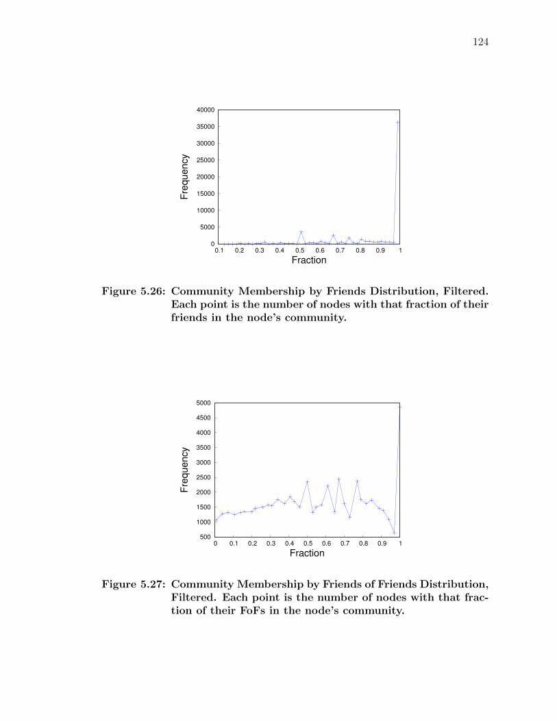
124
0
5000
10000
15000
20000
25000
30000
35000
40000
0.1 0.2 0.3 0.4 0.5 0.6 0.7 0.8 0.9 1
Fre
quency
Fraction
Figure 5.26: Community Membership by Friends Distribution, Filtered.Each point is the number of nodes with that fraction of theirfriends in the node’s community.
500
1000
1500
2000
2500
3000
3500
4000
4500
5000
0 0.1 0.2 0.3 0.4 0.5 0.6 0.7 0.8 0.9 1
Fre
quency
Fraction
Figure 5.27: Community Membership by Friends of Friends Distribution,Filtered. Each point is the number of nodes with that frac-tion of their FoFs in the node’s community.

125
0
5000
10000
15000
20000
25000
0 0.1 0.2 0.3 0.4 0.5 0.6 0.7 0.8 0.9 1
Fre
quency
Fraction
Figure 5.28: Friends Within Community Distribution, Filtered. Eachpoint is the number of nodes with that fraction of theircommunity being friends of the node.
0
2000
4000
6000
8000
10000
12000
0 0.1 0.2 0.3 0.4 0.5 0.6 0.7 0.8 0.9 1
Fre
quency
Fraction
Figure 5.29: Friend of Friends Within Community Distribution, Filtered.Each point is the number of nodes with that fraction of theircommunity being friends of friends of the node.

CHAPTER 6
Conclusion
To summarize, we considered three situations, the individual merits of which are
summarized in Section 6.1. The thread that tied them together was that all three
topics focus on effects driven by human actions with spatial context. These move-
ments are not based on any one individual independently, but are a function of
social interactions. In each case we find that to understand the research problem,
we must consider these interactions and the underlying relationships. While our
findings support the claim that social network features contribute meaningfully to
our understanding, our work is by no means comprehensive. We discuss limitations
in our findings in Section 6.2 and options for future work in Section 6.3.
6.1 Contributions
In Chapter 3, we explored the task of participatory sensing, first through an
examination of related systems and then by designing a simulation. Within the
simulation we used a quantitative approach by framing the system as a recurring
reverse auction, and studying the battery level and cost of measurements across sev-
eral market mechanisms applied to virtual rational players. While the dissertation
does not go into depth on the results in our previous work, [48], we continue where
that work left off by addressing the unrealistic random mobility model that had been
employed. Using a model based on real-world taxi traces in San Francisco [50, 51],
we showed that by incorporating human mobility, the market composition was com-
pletely different from what had been seen in our previous work. Furthermore, this
mobility meant there were both times where the system simply would not receive
data, and that the load on individuals as well the sensing campaign’s budget were
affected by when and where individuals were.
Next in Chapter 4, we set out to try and use a location-based social network,
Gowalla, to model economic performance in the United States. We considered three
metrics: GDP, Patents, and Startups, and found that GDP was reasonably well
126

127
described by a combination of our indicators, including population which is known to
correlate with GDP. In particular we found that long ties contributed to estimations,
which we believe is a result of idea flow and subsequent innovation being more readily
transferred through bridges (weak ties) which have a higher concentration of long
ties than short ties. On the other hand Patents and Startups didn’t map as easily,
possibly due to the nature of both data sets. In addition to our results, which
demonstrated that a network feature could provide additional insight, we also had
to design our MLE approximation which took considerable mathematical treatment.
Interestingly, in our design, we established a relationship between the Exponential
estimation and the Gaussian estimation.
Finally in Chapter 5, we designed an artificial social search by again using
Gowalla data [67], and drawing design inspiration from the famous Milgram small-
world experiments. Within our search we were able to again design several protocols
a rational searcher might follow, and explore the effects of partial knowledge of the
network structure and protocols on the efficiency of a social search. We were not
concerned with efficiency of the search for the sake of finding short paths, but did
study the chain lengths alongside success rates to understand how the search be-
haved. We found that even a small amount of friend-of-friend (FoF) knowledge
(using our parameter κ) significantly improved methods that were not community-
driven. Community information in this context was actually quite powerful. Since
community membership is a feature that was binary and nodes in a common com-
munity likely shared more links by definition, using this information could exclude
many less desirable candidate nodes from forwarding decisions than distance or pop-
ularity could. Ultimately, how effective a searcher a node was described by both how
well connected that individual was, and the knowledge at their disposal to refine
where the packet would travel to next.
6.2 Limitations
In Chapter 3, we utilized a taxi-based mobility model. While the movements
of taxis are requested by customers, we treat each taxi as a participant based on
the taxi’s identity as opposed to based on an individual traveler’s identity. This

128
is not an ideal model, since it associates the movement with the taxi drivers and
doesn’t show what happens when participants are outside of cabs. In general, it
is a challenging problem to get a timestamped mobility trace of even a moderate
number of individuals, so finding suitable data to better represent human mobility
remains a large challenge.
One of the metrics we examined in Chapter 4 was startups. However we
did not restrict startups by sector, so part of our difficulty in modeling startups
may have stemmed from including less innovative sectors that either do not require
many novel ideas or are in fields that advance slowly like services. Our approach to
distinguishing ties in all three cases was to examine just long ties and short ties based
on state boundaries. However, since the Gowalla population is highly concentrated
in metropolitan areas that account for only a small fraction of the area in the U.S.,
the effect may have been driven by bridging metropolitan regions as opposed to
states.
The users in the Gowalla data used in Chapters 4-5 were not a perfect repre-
sentation of the U.S. population. As we explained earlier in the dissertation, they
are likely to be of better than average socioeconomic standing and be inclined to-
wards innovation and early adoption of new products. Furthermore they exhibit a
willingness to share location, which may lead them to being more connected or more
informed in the context of social searches.
We found that community membership was a very important criterion for per-
forming social searches in Chapter 5, however these communities were arbitrarily
produced by an algorithm. In the real world communities are usually based on
a shared interest or activity such as ‘friends of [a popular individual],’ ‘fans of [a
sports team],’ ‘photographers,’ and so on. In an artificial social search where the
communities are not predefined, the efficacy of communities is dependent on the par-
titioning, and we have no way to readily evaluate the accuracy of our communities.
Additionally, we only consider the case of non-overlapping communities.
Finally, we claimed in Chapter 5 that the order in which protocols were used
mattered, and that properties specific to each network would likely impact the per-
formance of a given permutation of criteria. This dependency, which stems from

129
a ‘series of filters’ approach, exists because we wanted to frame the emulation in
a way that would be accessible to human reasoning. In an artificial environment
where human reasoning was not considered, our approach would likely be inferior
to an approach that could utilize all relevant criteria simultaneously.
6.3 Future Work
In Chapter 3, all of experiments were done in simulation. Real world experi-
ments would be a useful extension to verify the behaviors we observed in our system
as well as test the system on true human mobility without the obstacles involved in
finding an already existing data set. If such a dataset was found, it could serve as
a weaker but much less costly method of validation, since a real experiment would
involve incentives, infrastructure, and development of an actual sensing platform in
hardware and software.
As mentioned in Section 6.2, the modeling done in Chapter 4 should be re-
examined in the context of ties that connect metropolitan areas instead of ties that
cross state boundaries. The number of ties, and thus the chance for ideas to be
produced, increase at a superlinear rate with respect to population, as described in
literature cited within that chapter. It follows that the most ideas are thus concen-
trated at theses greater metropolitan areas, and that connecting two metropolitan
areas would thus have the strongest chance of catalyzing development through in-
novation.
While a potentially small extension to our work in Chapter 5 would be using
overlapping communities, the more prominent extension would be to replace the cur-
rent hybridization of protocols with an order-agnostic variant. Instead of computing
for example, the best choice based on distance, then the best remaining choice based
on communities, etc., a search utility score for each node could be computed from
a weighted vector of all relevant criteria. The approach would have to tune these
weights, either globally or through learning over the course of one or more trials.

REFERENCES
[1] U. of California, Berkely, (2011, Mar.) “Mobile millennium.” [Online].Available: http://traffic.berkeley.edu Accessed on Oct. 14, 2016.
[2] S. B. Eisenman et al., “Bikenet: A mobile sensing system for cyclist experiencemapping,” ACM Trans. Sen. Netw., vol. 6, no. 1, pp. 6:1–6:39, Jan. 2010.
[3] M. A. Alswailim, H. S. Hassanein, and M. Zulkernine, (2015, Nov.) “CRAW-DAD dataset queensu/crowd temperature (v. 2015-11-20).” [Online]. Available:http://crawdad.org/queensu/crowd temperature/20151120 Accessed on Oct.16, 2016.
[4] D. Trossen and D. Pavel, “Nors: an open source platform to facilitate partici-patory sensing with mobile phones,” in 4th Annu. Int. Conf. Mobile UbiquitousSyst.: Networking Services, Philadelphia, PA, 2007, pp. 1–8.
[5] P. Juang et al., “Energy-efficient computing for wildlife tracking: design trade-offs and early experiences with zebranet,” SIGOPS Oper. Syst. Rev., vol. 36,no. 5, pp. 96–107, Oct. 2002.
[6] S. Reddy, D. Estrin, M. Hansen, and M. Srivastava, “Examining micro-payments for participatory sensing data collections,” in Proc. 12th ACM Int.Conf. Ubiquitous Computing, Copenhagen, Denmark, 2010, pp. 33–36.
[7] J.-S. Lee and B. Hoh, “Dynamic pricing incentive for participatory sensing,”Pervasive and Mobile Computing, vol. 6, no. 6, pp. 693 – 708, Dec. 2010.
[8] K. Shilton, J. A. Burke, D. Estrin, M. Hansen, and M. Srivastava,(2008, Apr.) “Participatory privacy in urban sensing.” [Online]. Available:http://www.escholarship.org/uc/item/90j149pp Accessed on Oct. 14, 2016.
[9] G. Mainland, D. C. Parkes, and M. Welsh, “Decentralized, adaptive resourceallocation for sensor networks,” in Proc. 2nd Conf. Symp. Networked Syst. De-sign Implementation, vol. 2. Berkeley, CA: USENIX Association, 2005, pp.315–328.
[10] S. H. Clearwater, Market-Based Control: A Paradigm for Distributed ResourceAllocation. River Edge, NJ: World Scientific Publishing Company, 1996.
[11] M. P. Wellman, “Market-oriented programming: Some early lessons,” inMarket-Based Control: A Paradigm for Distributed Resource Allocation. RiverEdge, NJ: World Scientific, 1996, pp. 74–95.
130
131
[12] R. S. Sutton and A. G. Barto, Reinforcement Learning: An Introduction. NewYork, NY: Cambridge Univ Press, 1998.
[13] K. Whitehouse, C. Sharp, E. Brewer, and D. Culler, “Hood: a neighborhoodabstraction for sensor networks,” in Proc. 2nd Int. Conf. Mobile Syst., Appl.,and Services, Boston, MA, 2004, pp. 99–110.
[14] E. Byrne and P. M. Alexander, “Questions of ethics: participatory informationsystems research in community settings,” in Proc. 2006 Annu. Res. Conf. SouthAfrican Inst. Computer Scientists Inform. Technologists IT Res. DevelopingCountries, Somerset West, South Africa, 2006, pp. 117–126.
[15] L. Palen and P. Dourish, “Unpacking privacy for a networked world,” in Proc.SIGCHI Conf. Human Factors Computing Syst., Ft. Lauderdale, FL, 2003, pp.129–136.
[16] A. Acquisti and R. Gross, “Imagined communities: Awareness, informationsharing, and privacy on the facebook,” in Privacy Enhancing Technologies,Lecture Notes in Computer Science, G. Danezis and P. Golle, Eds. Berlin,Germany: Springer Berlin Heidelberg, June 2006, vol. 4258, pp. 36–58.
[17] K. L. Huang, S. S. Kanhere, and W. Hu, “Preserving privacy in participatorysensing systems,” Comput. Commun., vol. 33, no. 11, pp. 1266 – 1280, July2010.
[18] G. Calandriello, P. Papadimitratos, J.-P. Hubaux, and A. Lioy, “Efficient androbust pseudonymous authentication in vanet,” in Proc. 4th ACM Int. Work-shop Veh. Ad Hoc Networks, Montreal, Quebec, Canada, 2007, pp. 19–28.
[19] K. P. Tang, P. Keyani, J. Fogarty, and J. I. Hong, “Putting people in theirplace: an anonymous and privacy-sensitive approach to collecting sensed data inlocation-based applications,” in Proc. SIGCHI Conf. Human Factors Comput.Syst., Montreal, Quebec, Canada, 2006, pp. 93–102.
[20] C. Cornelius et al., “Anonysense: privacy-aware people-centric sensing,” in Proc.6th Int. Conf. Mobile Syst., Appl., Services, Breckenridge, CO, 2008, pp. 211–224.
[21] L. Sweeney, “k-anonymity: A model for protecting privacy,” Int. J. Uncertainty,Fuzziness Knowledge-Based Syst., vol. 10, no. 05, pp. 557–570, Oct. 2002.
[22] J. Domingo-Ferrer and J. Mateo-Sanz, “Practical data-oriented microaggrega-tion for statistical disclosure control,” IEEE Trans. Knowl. Data Eng., vol. 14,no. 1, pp. 189–201, Jan./Feb. 2002.
[23] A. Machanavajjhala, D. Kifer, J. Gehrke, and M. Venkitasubramaniam, “L-diversity: Privacy beyond k-anonymity,” ACM Trans. Knowl. Discov. Data,vol. 1, no. 1, pp. 1–52, Mar. 2007.

132
[24] H. Jian-min, C. Ting-ting, and Y. Hui-qun, “An improved v-mdav algorithmfor l-diversity,” in 2008 Int. Symp. Inform. Process., Moscow, Russia, 2008, pp.733–739.
[25] D. Kotz, T. Henderson, I. Abyzov, and J. Yeo, (2009, Sep.) “CRAWDADdata set dartmouth/campus (v. 2009-09-09).” [Online]. Available: http://crawdad.cs.dartmouth.edu/dartmouth/campus Accessed on Oct. 15, 2016.
[26] R. K. Ganti, N. Pham, Y.-E. Tsai, and T. F. Abdelzaher, “Poolview: streamprivacy for grassroots participatory sensing,” in Proc. 6th ACM Conf. EmbeddedNetwork Sensor Syst., Raleigh, NC, 2008, pp. 281–294.
[27] A. Tikhonov, A. Goncharsky, V. Stepanov, and A. G. Yagola, Numerical Meth-ods for the Solution of Ill-Posed Problems. Dordrecht, Netherlands: SpringerScience+Business Media B.V., 1995.
[28] C. Guestrin, P. Bodik, R. Thibaux, M. Paskin, and S. Madden, “Distributedregression: an efficient framework for modeling sensor network data,” in 3rdInt. Symp. Inform. Process. Sensor Networks, Berkeley, CA, 2004, pp. 1–10.
[29] B. Hull et al., “Cartel: a distributed mobile sensor computing system,” in Proc.4th Int. Conf. Embedded Networked Sensor Syst., Boulder, CO, 2006, pp. 125–138.
[30] V. Bychkovsky, B. Hull, A. Miu, H. Balakrishnan, and S. Madden, “A measure-ment study of vehicular internet access using in situ wi-fi networks,” in Proc.12th Annu. Int. Conf. Mobile Computing Networking, Los Angeles, CA, 2006,pp. 50–61.
[31] T. Small and Z. J. Haas, “The shared wireless infostation model: a new ad hocnetworking paradigm (or where there is a whale, there is a way),” in Proc. 4thACM Int. Symp. Mobile Ad Hoc Networking Computing, Annapolis, MD, 2003,pp. 233–244.
[32] M. S. Granovetter, “The strength of weak ties,” Amer. J. Sociology, vol. 78,no. 6, pp. 1360–1380, May 1973.
[33] W. Gao, Q. Li, B. Zhao, and G. Cao, “Multicasting in delay tolerant networks:A social network perspective,” in Proc. 10th ACM Int. Symp. Mobile Ad HocNetworking Computing, New Orleans, LA, 2009, pp. 299–308.
[34] S. Milgram, “The small world problem,” Psychology Today, vol. 2, no. 1, pp.60–67, May 1967.
[35] J. Travers and S. Milgram, “An experimental study of the small world problem,”Sociometry, vol. 32, no. 4, pp. 425–443, Dec. 1969.

133
[36] S. Schnettler, “A structured overview of 50 years of small-world research,”Social Networks, vol. 31, no. 3, pp. 165–178, July 2009.
[37] C. Korte and S. Milgram, “Acquaintance networks between racial groups: Ap-plication of the small world method,” J. Personality Social Psychology, vol. 15,no. 2, p. 101, June 1970.
[38] P. S. Dodds, R. Muhamad, and D. J. Watts, “An experimental study of searchin global social networks,” Sci., vol. 301, no. 5634, pp. 827–829, Aug. 2003.
[39] M. Chu, H. Haussecker, and F. Zhao, “Scalable information-driven sensor query-ing and routing for ad hoc heterogeneous sensor networks,” Int. J. High Per-formance Computing Appl., vol. 16, no. 3, pp. 293–313, Aug. 2002.
[40] S. Reddy, D. Estrin, M. Hansen, and M. Srivastava, “Examining micro-payments for participatory sensing data collections,” in Proc. 12th ACM Int.Conf. Ubiquitous Computing, Copenhagen, Denmark, 2010, pp. 33–36.
[41] S. Reddy, D. Estrin, and M. Srivastava, “Recruitment framework for partici-patory sensing data collections,” in Proc. 8th Int. Conf. Pervasive Computing,Helsinki, Finland, 2010, pp. 138–155.
[42] V. Krishna, Auction Theory. Cambridge, MA: Academic Press/Elsevier, 2009.
[43] G. Pickard et al., “Time-critical social mobilization,” Sci., vol. 334, no. 6055,pp. 509–512, Oct. 2011.
[44] J.-S. Lee and B. K. Szymanski, “A novel auction mechanism for selling time-sensitive e-services,” in 7th IEEE Int. Conf. E-Commerce Technol., Xi’an,China, 2005, pp. 75–82.
[45] J.-S. Lee and B. K. Szymanski, “Stabilizing markets via a novel auctionbased pricing mechanism for short-term contracts for network services,” in 9thIFIP/IEEE Int. Symp. Integrated Network Manage., Nice, France, 2005, pp.367–380.
[46] J. Grossklags and A. Acquisti, “When 25 cents is too much: An experimenton willingness-to-sell and willingness-to-protect personal information,” in Proc.6th Workshop Econ. Inform. Security, Pittsburgh, PA, 2007, pp. 7–8.
[47] P. Gilbert, L. P. Cox, J. Jung, and D. Wetherall, “Toward trustworthy mobilesensing,” in Proc. 11th Workshop Mobile Computing Syst. Appl., Annapolis,MD, 2010, pp. 31–36.
[48] B. O. Holzbauer, B. K. Szymanski, and E. Bulut, “Socially-aware market mech-anism for participatory sensing,” in Proc. 1st ACM Int. Workshop Mission-oriented Wireless Sensor Networking, Istanbul, Turkey, Aug. 2012, pp. 9–14.

134
[49] J.-S. Lee and B. K. Szymanski, “A participation incentive market mechanismfor allocating heterogeneous network services,” in Proc. 28th IEEE Conf. GlobalTelecommun., Honolulu, HI, Nov. 2009, pp. 2206–2211.
[50] M. Piorkowski, N. Sarafijanovic-Djukic, and M. Grossglauser, (2009, Feb.)“CRAWDAD data set epfl/mobility (v. 2009-02-24).” [Online]. Available:http://crawdad.cs.dartmouth.edu/epfl/mobility Accessed on Oct. 15, 2016.
[51] M. Piorkowski, N. Sarafijanovoc-Djukic, and M. Grossglauser, “A ParsimoniousModel of Mobile Partitioned Networks with Clustering,” in 1st Int. Conf. Com-mun. Syst. Networks, Bangalore, India, 2009.
[52] E. A. Boxman, P. M. De Graaf, and H. D. Flap, “The impact of social andhuman capital on the income attainment of dutch managers,” Social Networks,vol. 13, no. 1, pp. 51–73, Mar. 1991.
[53] R. S. Burt, “Structural holes and good ideas,” Amer. J. Sociology, vol. 110,no. 2, pp. 349–399, Sept. 2004.
[54] R. S. Burt, Structural Holes: The Social Structure of Competition. Cambridge,MA: Harvard University Press, 2009.
[55] M. Granovetter, Getting a Job: A Study of Contacts and Careers. Chicago,IL: University of Chicago Press, 1995.
[56] M. Granovetter, “The impact of social structure on economic outcomes,” J.Econ. Perspectives, vol. 19, no. 1, pp. 33–50, Jan. 2005.
[57] R. Reagans and E. W. Zuckerman, “Networks, diversity, and productivity: Thesocial capital of corporate r&d teams,” Org. Sci., vol. 12, no. 4, pp. 502–517,July/Aug. 2001.
[58] M. Ruef, “Strong ties, weak ties and islands: structural and cultural predictorsof organizational innovation,” Ind. Corporate Change, vol. 11, no. 3, pp. 427–449, June 2002.
[59] A. Pentland, Social Physics: How Good Ideas Spread – the Lessons From a NewScience. New York, NY: Penguin Books, 2014.
[60] L. Adamic and E. Adar, “How to search a social network,” Social Networks,vol. 27, no. 3, pp. 187–203, July 2005.
[61] J. Kleinberg, “The small-world phenomenon: An algorithmic perspective,” inProc. 32nd Annu. ACM Symp. Theory Computing. Portland, OR: ACM, 2000,pp. 163–170.
[62] D. Liben-Nowell, J. Novak, R. Kumar, P. Raghavan, and A. Tomkins, “Geo-graphic routing in social networks,” Proc. Nat. Academy Sciences United StatesAmerica, vol. 102, no. 33, pp. 11 623–11 628, Aug. 2005.

135
[63] D. J. Watts, P. S. Dodds, and M. E. Newman, “Identity and search in socialnetworks,” Sci., vol. 296, no. 5571, pp. 1302–1305, May 2002.
[64] L. Bettencourt and G. West, “A unified theory of urban living,” Nature, vol.467, no. 7318, pp. 912–913, Oct. 2010.
[65] L. M. Bettencourt, J. Lobo, D. Helbing, C. Kuhnert, and G. B. West, “Growth,innovation, scaling, and the pace of life in cities,” Proc. Nat. Academy Sciences,vol. 104, no. 17, pp. 7301–7306, Apr. 2007.
[66] W. Pan, G. Ghoshal, C. Krumme, M. Cebrian, and A. Pentland, “Urbancharacteristics attributable to density-driven tie formation,” Nature Commun.,vol. 4, June 2013. [Online]. Available: http://www.nature.com/articles/ncomms2961
[67] T. Nguyen and B. K. Szymanski, “Using location-based social networks tovalidate human mobility and relationships models,” in IEEE/ACM Int. Conf.Advances Social Networks Anal. Mining, Istanbul, Turkey, 2012, pp. 1215–1221.
[68] T. Nguyen, M. Chen, and B. K. Szymanski, “Analyzing the proximity andinteractions of friends in communities in gowalla,” in 2013 IEEE 13th Int.Conf. Data Mining Workshops, Dallas, TX, 2013, pp. 1036–1044.
[69] D. Centola and M. Macy, “Complex contagions and the weakness of long ties,”Amer. J. Sociology, vol. 113, no. 3, pp. 702–734, Nov. 2007.
[70] G. Ghasemiesfeh, R. Ebrahimi, and J. Gao, “Complex contagion and the weak-ness of long ties in social networks: revisited,” in Proc. 14th ACM Conf. Elec-tron. Commerce, Philadelphia, PA, 2013, pp. 507–524.
[71] N. Eagle, M. Macy, and R. Claxton, “Network diversity and economic develop-ment,” Sci., vol. 328, no. 5981, pp. 1029–1031, May 2010.
[72] A. Tacchella, M. Cristelli, G. Caldarelli, A. Gabrielli, and L. Pietronero, “A newmetrics for countries’ fitness and products’ complexity,” Sci. Reports, vol. 2,Oct. 2012. [Online]. Available: http://www.nature.com/articles/srep00723
[73] U.S. Bureau. of Economic Analysis, (2015) “Advance 2014 and revised1997-2013 statistics of gdp by state.” [Online]. Available: http://www.bea.gov/newsreleases/regional/gdp state/2015/gsp0615.htm Accessed on Sept. 28,2015.
[74] U.S. Patent and Trademark Office, Patent Technology Monitoring Team,(2015) “Patent counts by country, state, and year - utility patents (december2015).” [Online]. Available: http://www.uspto.gov/web/offices/ac/ido/oeip/taf/cst utl.htm Accessed Sept. 28, 2015].
136
[75] U.S. Census Bureau, Statistics of U.S. Businesses (SUSB), (2015) “2012 susbannual datasets by establishment industry.” [Online]. Available: http://www.census.gov/data/datasets/2012/econ/susb/2012-susb.html Accessed on Sept.28, 2015.
[76] J. Xie and B. Szymanski, “Labelrank: A stabilized label propagation algorithmfor community detection in networks,” in IEEE 2nd Network Sci. Workshop,West Point, NY, 2013, pp. 138–143.
[77] T. Nguyen, “Proximity, interactions, and communities in social networks : prop-erties and applications,” Ph.D. dissertation, Dept. of Comput. Sci., RensselaerPolytechnic Inst., Troy, NY, 2014.
[78] L. A. Adamic and E. Adar, “Friends and neighbors on the web,” SocialNetworks, vol. 25, no. 3, pp. 211–230, July 2003. [Online]. Available:http://www.sciencedirect.com/science/article/pii/S0378873303000091
[79] D. Liben-Nowell and J. Kleinberg, “The link-prediction problem for socialnetworks,” J. Amer. Soc. Inform. Sci. Technol., vol. 58, no. 7, pp. 1019–1031,Mar. 2007. [Online]. Available: http://dx.doi.org/10.1002/asi.20591
[80] A. P. Dempster, N. M. Laird, and D. B. Rubin, “Maximum likelihood from in-complete data via the em algorithm,” J. Roy. Statistical Soc. Series B (Method-ological), vol. 39, no. 1, pp. 1–38, Jan. 1977.
[81] B. O. Holzbauer, B. K. Szymanski, T. Nguyen, and A. Pentland, “Social tiesas predictors of economic development,” in Int. Conf. School Network Sci.,Wroc law, Poland, 2016, pp. 178–185.
[82] K. Burnham and D. Anderson, Model Selection and Inference: A PracticalInformation-theoretic Approach. New York, NY: Springer, 1998.
[83] L. Backstrom, P. Boldi, M. Rosa, J. Ugander, and S. Vigna, “Four degrees ofseparation,” in Proc. 4th Annu. ACM Web Sci. Conf., Evanston, IL, 2012, pp.33–42.
[84] Y.-Y. Ahn, S. Han, H. Kwak, S. Moon, and H. Jeong, “Analysis of topologicalcharacteristics of huge online social networking services,” in Proc. 16th Int.Conf. World Wide Web, Banff, Canada, 2007, pp. 835–844.
[85] H. Kwak, C. Lee, H. Park, and S. Moon, “What is twitter, a social network ora news media?” in Proc. 19th Int. Conf. World Wide Web, Raleigh, NC, 2010,pp. 591–600.
[86] A. Mislove, M. Marcon, K. P. Gummadi, P. Druschel, and B. Bhattacharjee,“Measurement and analysis of online social networks,” in Proc. 7th ACM SIG-COMM Conf. Internet Measurement, San Diego, CA, 2007, pp. 29–42.

137
[87] A.-L. Barabasi, R. Albert, and H. Jeong, “Scale-free characteristics of randomnetworks: the topology of the world-wide web,” Physica A: Statistical MechanicsIts Appl., vol. 281, no. 1, pp. 69–77, June 2000.
[88] A.-L. Barabasi, Network Science. Cambridge, MA: Cambridge UniversityPress, 2016.
[89] J. Urry, “Small worlds and the new social physics,” Global Networks, vol. 4,no. 2, pp. 109–130, Apr. 2004.
[90] B. O. Holzbauer, B. K. Szymanski, and E. Bulut, “Incentivizing participa-tory sensing via auction mechanisms,” in Opportunistic Mobile Social Networks.Boca Raton, FL: CRC Press, 2014, ch. 12, pp. 339–736.