ISSN: 1439-2305

Number 69 – January 2008

How effective are poor schools?

Poverty and educational outcomes

in South Africa

Servaas Van der Berg

How effective are poor schools? Poverty and educational outcomes in South Africa1*

Servaas van der Berg Department of Economics University of Stellenbosch

Stellenbosch South Africa

Email: SvdB@sun.ac.za

Abstract Massive differentials on achievement tests and examinations reflect South Africa’s

divided past. Improving the distribution of educational outcomes is imperative to overcome labour market inequalities. Historically white and Indian schools still outperform black and coloured schools in examinations, and intraclass correlation coefficients (rho) reflect far greater between-school variance compared to overall variance than for other countries.

SACMEQ’s rich data sets provide new possibilities for investigating relationships between educational outcomes, socio-economic status (SES), pupil and teacher characteristics, school resources and school processes. As a different data generating process applied in affluent historically white schools (test scores showed bimodal distributions), part of the analysis excluded such schools, sharply reducing rho. Test scores were regressed on various SES measures and school inputs for the full and reduced sample, using survey regression and hierarchical (multilevel) (HLM) models to deal with sample design and nested data. This shows that the school system was not yet systematically able to overcome inherited socio-economic disadvantage, and poor schools least so. Schools diverged in their ability to convert inputs into outcomes, with large standard deviations for random effects in the HLM models. The models explained three quarters of the large between-school variance but little of the smaller within-school variance. Outside of the richest schools, SES had only a mild impact on test scores, which were quite low in SACMEQ context. JEL Classification: J210 Keywords: Analysis of Education

1 Revised version of paper delivered at SACMEQ International Invitational Research Conference, Paris,

September 2005. The author wishes to thank Derek Yu for technical assistance with the data and Megan Louw,

Ronelle Burger, Kenneth Ross and Neville Postlethwaite for useful comments.

* The paper has been presented at the cege research colloquium, University of Göttingen, November 2007.

2

Introduction

Massive differentials on achievement tests and examinations reflect South Africa’s

divided past. Despite narrowing attainment differentials, unprecedented resource transfers to

black schools and large inflows of black pupils to historically white schools, studies have

shown that historically white and Indian schools still far outperform black and coloured

schools in matriculation examinations and performance tests at various levels of the school

system. Moreover South African educational quality lags far behind even much poorer

countries, as has been demonstrated by a number of international tests, including MLA,

TIMSS and now SACMEQ II. Educational quality in historically black schools – which

constitute 80 per cent of enrolment and are thus central to educational progress – has not

improved significantly since political transition. Inadequate educational progress constrains

both black upward mobility in the labour market and the skills required for economic growth

in a middle-income country.

Thus a better understanding is required of the factors that inhibit performance in

poorer, mainly black or coloured schools. This paper attempts to improve understanding of

the role of socio-economic status (SES) and other factors in determining educational

performance at the Grade 6 level. Such performance affects drop-outs, transitions between

grades and quality of educational performance up to matriculation and beyond.

Studies have shown high variability in school performance (large residuals) after

controlling for SES and teacher inputs that may be indicative of varying efficiency, hinting at

managerial problems in many schools (Crouch and Mabogoane 1998). Because of data

limitations, education production function studies thus far have had to use school examination

performance for matriculation (Grade 12) and have largely ignored non-teacher school inputs

and processes. SACMEQ II’s rich individual and school level data provide new possibilities

for investigating interactions between educational outcomes, SES, school resources and

teacher inputs, thus moving towards an understanding of how and under which conditions

resources improve outcomes. As it appears that quite different processes may determine

learning outcomes in affluent schools (bimodal distributions of test scores provide evidence of

separate data generating processes) and the focus here lies predominantly on the performance

of the resource-scarce formerly black school system, part of the analysis excludes affluent

schools. Test scores will be regressed on SES, pupil characteristics, school inputs, school

processes and location for the full and reduced sample, using Stata’s survey regression and

hierarchical (multilevel) (HLM) models to deal with sample design and nested data. This

should help to advance understanding of the conditions required for resources to have an

3

optimal impact, as earlier work indicated that resources mattered only conditionally on school

efficiency (the ability to convert resources into educational performance, whilst controlling

for SES),), which varied widely amongst schools.

The paper proceeds in the following way: First, South African educational inequality

between schools is discussed and placed in international perspective, to show that such

inequality is indeed a large part of the education challenge in this country. The paper then

turns to a brief discussion of the SACMEQ II South African data. Thereafter, an analysis of

performance is attempted by focusing on both school and pupil performance, using OLS

(ordinary least-square) regressions but allowing for clustering effects in sample design. The

next step is an analysis of performance of poorer schools (a reduced sample), to try to exclude

most formerly white schools that could perhaps best be seen as functioning on the basis of a

different data generating process. This procedure assists in capturing the relationships

amongst individuals in schools that were not formerly advantaged, so that the coefficients can

better be interpreted as applying amongst such schools. If the same analysis was applied to all

schools, then the coefficients would instead reflect differences between historically white and

historically black schools. Next, quantile regression is used for the same purpose, viz. to

model the differences between performance of children in well and weakly performing

schools. School rather than individual performance is briefly modelled next, as a prelude to

the final modelling. The final form of analysis employed here is the estimation of a two-level

HLM which attempts to incorporate the effects of both individual and school characteristics,

focusing particularly on the role of SES. The paper closes with an overall conclusion.

Inequality between schools

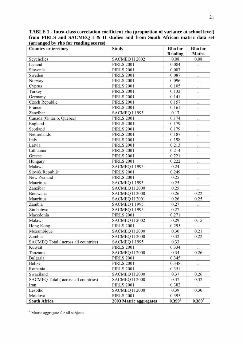
The intraclass correlation coefficient rho (ρ) – which expresses the variance in

performance between schools as a proportion of overall variance – is extremely high in South

Africa. The Kenya SACMEQ II report (SACMEQ 2005: Ch.8, p.14) quotes Willms and

Somers’ (2001) finding that the intraclass correlation coefficient ranged from 19.5 per cent to

41.2 per cent for mathematics achievement for Grade 3 and 5 pupils in 13 Latin American

countries. Rumberger and Palardy (2003: 14) report a value of 25 per cent to be “within the

range that Coleman found in his 1996 study and the range found in other recent studies of

student achievement using similar models”. In calculating required sample sizes, SACMEQ II

erroneously assumed that rho for the group of countries investigated would be in the range of

0.3 to 0.4, thus underestimating the number of schools that needed to be sampled for the

desired significance (Ross, Saito, Dolata, Ikeda, Zuze, Murimba, Postlethwaite and Griffin

4

2005: 26). Table 1 below shows the range of this magnitude from three sets of international

studies, arranged by the rho values for the reading scores in cases where both reading and

mathematics were tested. The SACMEQ 2000 rho values of 0.70 for South Africa’s reading

scores and 0.64 for the mathematics scores confirm that inequality in performance between

schools in South Africa is exceedingly high. South Africa has by far the highest recorded

values, with Namibia its closest rival by this measure of the degree to which inequality

applies between rather than within schools. Although the intraclass correlation for the 2003

matriculation results is considerably lower at 0.3992, it is unlikely that this means that the

SACMEQ data overestimated the South African rho: An unpublished Western Cape study at

primary school level also found a value of 0.72 for reading, but a much lower value for

mathematics (0.44), perhaps reflecting more individual variation in mathematics performance.

This high degree of inequality between schools is largely a legacy of historical

educational inequality. However, it arises more from differences in educational quality than

from differential attainment, since the latter has narrowed considerably in recent decades.

Indeed, Lam (1999) found that South African attainment differentials between race groups

had narrowed faster than in Brazil – a country with income inequality levels similar to South

Africa’s.

The differentials in performance between high and low SES groups, or rich and poor,

far exceeded that in other SACMEQ countries in both reading and mathematics, judging by

the SACMEQ indicators and their SES measure (SACMEC Indicators 2005). The differences

in mean scores of rich and poor shown in Figure 1 illustrate how far South Africa leads the

field in this measure of educational inequality. Namibia (for reading) and Mauritius (for

mathematics) were closest to South African differentials between rich and poor. Figure 2

shows a similar picture, for the differential in scores between large cites and isolated rural

areas. Here, South African differentials were massive: there was urban-rural gap (as here

defined) of almost 180 score points for reading and almost 140 for mathematics. This is put

2 This may reflect one or both of these factors:

• Differences in transition and drop out rates, that prevent weaker pupils from reaching matric, thus reducing

variance both within and particularly between schools.

• Weaker quality differentiation in the matric examination, due to the wide subject choice allowed. However,

the intraclass correlation coefficient of the Mathematics mark of those who did take this subject was only

0.389 in 2003 (the Standard Grade mark converted to Higher Grade by subtracting 10 percentage points).

But this value was also reduced by self-selection: Those who were weaker at mathematics avoided the

subject.

5

into perspective when one considers that mean test scores have been set at 500 and the

standard deviation at 100 across all SACMEQ countries, and that only Namibia had

differentials more than half as large. The differentials also did not arise so much from

exceptional performance of the rich or the urban populations than from relatively poor

performance amongst the poor and those in isolated rural areas. This weak educational

performance of large segments of the population is put into further perspective when it is

considered that South Africa had a much higher per capita income than most SACMEQ

countries.

Lowess (locally weighted) regressions of the relationship between the SES derived for

this study (discussed below) and test scores had very similar shapes for individuals and school

averages for both reading and mathematics (Figures 3a, 3b, 4a and 4b). This relationship was

quite flat over most of its range, particularly for individuals. Apparently, SES only started

playing a role at a higher, threshold level of SES. At low levels of SES, individuals and

indeed schools did not seem to gain much in terms of reading or mathematics score

improvement from higher SES. This may indicate that most schools were not able to turn

higher SES, at least up to that threshold, into educational advantage. This cannot be taken as

evidence that such schools performed well in enabling poor children to perform almost as

well as those from middle class backgrounds, as these scores were low in SACMEQ

perspective. It was rather the case that the ineffectiveness of these schools meant that not even

middle class children performed well. Many of the individuals above the SES threshold level

were white and Indian pupils (slightly more than 10 per cent of national school enrolment,

though because of varying school size it is uncertain what proportion of schools they

constituted) who were historically clustered in schools that performed much better than

average. These schools had been racially desegregated, but still largely served the highest SES

groups. Based mainly on evidence for secondary schools (i.e. matriculation results), it has

been argued that such schools still far outperform others (Van der Berg & Burger, 2003). The

data shown here indicate that this argument also applied at primary school level.

The differentials in performance are also shown by school quintiles, where schools are

arranged according to their mean SES. Table 2 shows that mean performance per quintile

remained very flat between the poorest and third poorest quintiles (for reading, it rose by only

6 per cent, with no difference in mathematics performance). From Quintiles 3 to 4,

performance rose a little more, by another 10 per cent for reading and 8 per cent for

mathematics. However, the richest quintile performed more than 25 per cent better than the

second richest quintile in both reading and mathematics. Clearly, the richest quintile of

6

schools far outperformed the rest. This makes s strong case for excluding them from the

sample for the analysis that focuses on non-affluent schools.

The table also shows that only a few more than one third of South African pupils

performed above the SACMEQ mean of 500 on each of the two tests. This proportion

increased strongly across the quintiles, with the largest jump occurring when moving from the

second richest to the richest quintile. The proportion of each quintile with marks below 400

(one standard deviation below the SACMEQ mean) remained very similar across the bottom

three quintiles for both reading and mathematics, but dropped to a negligible share in the

richest quintile.

The data

The SACMEQ II survey was conducted mainly in 2000 in 14 countries of Southern and

Eastern Africa by the Southern African Consortium on Monitoring Education Quality, based

on complex two-stage clustered samples. Questionnaires were administered to selected pupils,

their reading and mathematics teachers, and their school principal. A chapter in the Kenya

SACMEQ report by Ross et al. (2005) provides more detail on sampling and all stages of the

process from the planning stage. In South Africa 169 schools were sampled, but because of

some missing values on some of the variables (mainly interviews with principals), the actual

sample in much of the analysis was reduced to 167 schools. Altogether 20 children in each

school were to be tested, but again there were a few missing observations for some variables

in the final data set. After allowing for these, the full sample of pupils stood at 3 163.

Applying pupil weights, this sample was broadly representative of the South African Grade 6

population, and – as almost universal school attendance had been achieved up to about age 16

– was also likely to be representative also of the 12 year old age group (note that repeaters and

those who started school early affected this slightly). However, SACMEQ acknowledged that

the effective sample (after taking cognisance of cluster effects in sample design) was smaller

for South Africa than is the norm: “In the SACMEQ II Project, two school systems, South

Africa and Uganda, fell far below the required target of an effective sample size of 400 pupils.

In South Africa the values were 185 and 230 for reading and mathematics, respectively …”

(Ross et al., 2005). This largely resulted from the intraclass correlation being larger than

allowed for in the sample design, thus too few South African schools were selected. In South

Africa. “Ministry concerns about the validity of sampling and measurement” were noted with

the release of the SACMEQ II data, leading to a delayed release of the data for this country

(see SACMEQ, 2004).

7

A large number of variables were generated by SACMEQ II, as described in more

detail in Ross et al. (2005) and elsewhere in the SACMEQ II Kenya Report (2005). These

variables were largely the ones used for this study, bearing in mind that in South Africa

teacher reading and mathematics skills were not tested (these skills were tested in all the other

SACMEQ countries). Furthermore, an own SES variable was created, as described below.

The main variables used in the analysis can be grouped as follows:

• Pupil-level variables: Pupil age, gender, number of times a grade was repeated, whether a

pupil always or sometimes spoke English at home3, education status of pupil’s parents,

whether the pupil lived with his/her parents, variables relating to the existence of various

household possessions, the materials the pupil’s home were constructed from, the school-

related items (e.g. pencils, rulers, etc) the pupil possesses, and the availability of

textbooks. In addition, information was also obtained on the pupil’s absence from school

and the reasons for such absence.

• Teacher-level variables: For both reading and mathematics, the teacher of each pupil was

interviewed to obtain information on gender, age, training, and some SES variables. As

not all pupils in each school sample came from the same class, in some schools more than

one teacher was interviewed in each subject.

• School variable: Information on the gender, age and training of school principals was

obtained, as well as information on reported school problems relating to pupils or

teachers.

• School resources: Classroom and other facilities, school building, and school equipment

were all recorded.

• School location: Three types of areas were distinguished, viz. large cities, towns, and

isolated rural areas.

• School processes: This included frequency of homework, frequency of correction of

homework, visits by inspectors, and test frequency.

Socio-economic status of pupils is an important determinant of learning outcomes. The

question in this case was how best to measure SES. The approach used by SACMEQ itself,

while useful, included parent education – which was regarded as an important regressor to

include separately in this study. A new SES variable was thus rather created, using the first

factor in principal component analysis that included as variables possessions in and services

used by the household (e.g. having a newspaper in the home, ownership of a radio, a 3 The test was conducted in English, one of South Africa’s eleven official languages, although only 14 per cent of pupils reported always speaking English at home.

8

television set, a fridge, a car, having electricity, a telephone), the type of house (judged by the

wall materials) and the quantity of a list of stationery items that the pupil had in school. The

SES variable constructed in this manner showed a high correlation with many of the variables

one would expect it to be associated with, whilst its average value was much higher for pupils

attending schools in large cities than those in towns or isolated rural areas.

The variables used are summarized in Table 3, along with their mean values, standard

deviations, minima and maxima.

Regression analysis: Full sample of individuals and schools

For the regression analysis, the broad underlying model was that SES, pupil

characteristics (age, gender, repeater status), access to textbooks, academic effort (as proxied

by homework frequency), teacher characteristics (age, gender, training, and tertiary

qualifications), school resources, school location, school processes, teacher and pupil

problems experienced in the school (violence, pupil behaviour, health, etc.) and perhaps also

the characteristics of the school principal may have played a role in determining learning

outcomes, in addition to the unobserved ability of the individual pupil. As ability was

unobserved, care should be taken in the interpretation of the models of possible ability bias

that may influence results. The modelling approach taken was general to specific, initially

including all variables deemed potentially relevant to the equation, but selectively dropping

those found not to be significant. A few control variables usually considered to be standard

explanatory variables in the education literature – including SES, pupil gender, mother’s

education, over age pupils, and provincial dummies (with NorthWest the reference province)

– were retained irrespective of their statistical significance or sign. As the sample of

individual children was clustered in schools, thus reducing heterogeneity, all regressions

adjusted for sample design and weighting of individuals using Stata’s survey regression

cluster option. Huber-White robust standard errors were generated to deal with possible

heteroskedasticity, thus ensuring stringent tests of variable significance.

The models fitted are as interesting for the variables that were retained as for those

that failed to enter the regressions significantly or with an appropriate sign – see Table 4,

regressions 1 and 2 for the full models for reading and mathematics respectively. Pupil SES

was an important predictor, but the effect appeared to be non-linear. A quadratic function

gave a better fit than a simple linear model for in both reading and mathematics, with SES

affecting scores little at low levels of SES, but playing an increasing role at higher SES levels,

as the lowess regressions had indicated may be the case. Other pupil characteristics that

9

played a role in explaining academic performance included gender, age, home language and

household structure. It is noticeable that males did worse on reading than females, but there

was no significant gender difference for mathematics. The gender dummy was nevertheless

retained as a control variable in all regressions. Overage children (above 12 years) performed

just over 20 marks worse on both the reading and mathematics scores, whilst underage

children had a disadvantage in mathematics. As the test was conducted in English, it was no

surprise that speaking English at home brought strong benefits in terms of performance. It is

interesting, however, that there was little difference between always speaking English at home

and sometimes doing so. In this country of highly fragmented family structures, pupils who

lived with their parents had a strong advantage in both reading and mathematics.

Turning to variables directly related to schooling, pupil attendance, grade repetition,

parents’ education and household resources appeared to be important determinants of

academic success. Pupil absence from school had the expected negative impact on marks, and

the effect was particularly large in the case of reading marks if such absence was due to

unpaid school fees4. As the model already controlled for SES and fees were quite low in most

schools, unpaid school fees probably partly proxied for a weaker commitment to education by

less affluent and probably less well educated parents. It did not appear as if repeating grades

brought pupils to the performance levels of their peers, as repeaters fared progressively worse

the more years of schooling they had repeated. Although the coefficients on the repetition

dummies were not all individually significant and did not show such a regular pattern for

mathematics, a joint significance test showed that they did have the expected combined effect.

Whilst having a mother with matric brought measurable benefits in terms of a child’s reading

performance, a child required his or her mother to have obtained at least a degree before the

benefits of maternal education were reflected in mathematics scores. By contrast, father’s

education did not show significant effects. The positive impact of having more than 10 books

at home was probably mainly another manifestation of home background, literacy and

attitudes to knowledge.

Not having an own textbook or having to share it with more than one other pupil was

associated with worse scores on reading. Interestingly, homework frequency did not lead to

any significant improvement in performance when the full sample was considered.

Equipment, measured on a scale of 0-11 (a count of the presence of a first aid kit, fax

machine, typewriter, duplicator, radio, tape recorder, overhead projector, TV, VCR,

4 Note that this result obtained even though schools were formally forbidden from applying sanctions against pupils whose fees were unpaid.

10

photocopier, and computer present in the school), played a positive role. In the case of

mathematics, school buildings (measured on a scale of 0-6: a count of the presence of a school

library, school hall, teacher room, office for school head, store room and cafeteria) also

impacted scores positively. Teacher training or tertiary qualifications did not enter the models

as significant factors. Urban schools in large cities performed much better than others, but

there was no indication that schools in towns performed better than those in isolated rural

areas. Where principals reported having teacher problems, reading scores were significantly

lower, although not by a large magnitude. The same result did not apply to mathematics

scores.

The pupil-teacher ratio (representing class size) did not significantly enter either of the

models, or entered them with the wrong sign, showing that the availability of this type of

resource was not as important as often thought. This confirmed earlier work that suggested

that teacher numbers play a limited role in South Africa (Crouch & Mabogoane 1998; Van der

Berg & Burger 2003), particularly since apartheid era disparities in the allocation of publicly

remunerated teachers between schools were eliminated. However, as in many other countries,

the quality of teachers may have been more important than the quantity in which they were

employed. Another relevant issue here was that, despite government’s attempts at

standardisation of the pupil-teacher ratio, two factors still contributed to maintaining de facto

disparities in this measure of school quality. Firstly, schools could impose school fees to

supplement public resources, and richer schools often used such funds to appoint teachers in

addition to those on the public payroll. Secondly, some schools may have had difficulty filling

positions – particularly schools located in deep rural areas. A factor that may have been even

more decisive for education quality in poor schools was that good teachers were likely to

prefer teaching in richer, urban schools. In view of the remaining differences in allocations of

publicly remunerated teachers and those appointed by the school governing body, the very

low correlation between mean SES of schools and pupil-teacher ratio or class size (for both, r

= –=0.17) was surprising. It is not clear whether this was the result of poor reporting on pupil-

teacher ratios, or whether factors other than teacher and pupil numbers (e.g. administrative

and other duties that kept some teachers out of classes) conflated the relationship between

class size and SES.

Regression analysis: Reduced samples

The intraclass correlation coefficient referred to earlier was substantially decreased if

the sample was reduced by first dropping the richest 10 per cent of schools (numbering 17)

11

from the sample, and then the next 10 per cent as well, as Table 1 shows. The affluence of a

school was measured by the mean SES of its pupils in the sample. The full sample reduction

reduced rho from 0.70 and 0.64 for reading and mathematics, to 0.47 and 0.39 respectively.

This large reduction reflected the fact that a major part of the educational performance

disparity in South Africa was between rich (mainly historically white and Indian) schools and

other schools. It may indicate that the superior performance of richer schools was due to both

having pupils with greater private resources (evidenced by a higher SES and having more

educated parents) that enhanced their schooling outcomes, and greater school efficiency in

converting school and pupil inputs into performance outcomes for pupils of any given SES.

Such conclusions about school efficiency in South Africa have been discussed before in

Crouch & Mabogoane (1998 & 2001) and Van der Berg & Burger (2002). If such schools do

operate differently, then there is a strong case for excluding white and Indian schools from the

sample for the regression analysis. Two separate data generating processes may indeed have

been at work, where the underlying statistical relationships would have been conflated by

treating them as one. If this conception of the world was correct, then the historically white

and Indian schools were best regarded as outliers which may have unduly influenced the

estimated coefficients in regressions estimated for the entire schooling system.

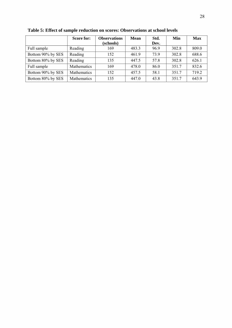
Table 5 shows the effect of reducing the sample in terms of scores at the school level.

Mean school SES scores drop quite considerably, but even more dramatic was the decline by

almost half in the standard deviation across schools. Note also that the maximum values

dropped precipitously.

There was no information on the former race-based department to which schools in the

sample belonged. However, it was known that race and SES were still highly correlated and

that historically white and Indian schools constituted a little more than 10 per cent of all

schools in South Africa. To remove these schools from the data set, the sample was reduced

twice in the manner described above: first the richest 10 per cent of schools were dropped,

and then the next 10 per cent The same parsimonious regression was then run on the original

sample as well as on the two reduced samples to see whether sample reduction strongly

affected the results.

If all the data captured the same underlying relationship, then the coefficients in the

three regressions should have been very similar. If on the other hand all former white and

Indian schools functioned quite dissimilarly according to a different data generating process,

and most were to be found in the top 10 or to 20 per cent of schools by SES, then the

estimated coefficients in either or both of the reduced samples should have differed

12

substantially from those in the original regression. This was indeed the case, as can be seen in

Table 6 for both the reading and mathematics scores: Regression equations altered

fundamentally when the sample was reduced. This was best illustrated by the magnitude of

the coefficient for SES, which declined for the reading scores from 9.022 in the full sample to

6.883 in the 10 per cent reduced sample and to 3.991 in the 20 per cent reduced sample. This

showed that the large and significant coefficient for SES in the original sample may perhaps

just have meant that richer (mainly historically white and Indian) schools performed much

better, since once they were removed from the sample, the effect of SES on test scores was

much smaller. For the mathematics score, the coefficient fell from 6.295 to 2.996, and finally

to 0.602. At this point, the coefficient was no longer statistically significant, indicating that

SES appeared to play no role in mathematics performance in historically mainly black and

coloured schools. The sharp change in the coefficients with both changes in the sample may

indicate that white and Indian schools were distributed across the top 20 per cent rather than

only the top 10 per cent of schools by SES in the sample. Other coefficients changed with the

sample reductions too, and in the case of mathematics scores even the urban dummy lost its

significance as a predictor of performance when more affluent schools were dropped.

The next step was to focus on the reduced sub-sample of mainly black and coloured

schools, so as to estimate the most appropriate regression models for this group of schools.

Separate models were fitted again in the same manner as before for reading and mathematics

scores. The results are shown in regressions 3 and 4 of Table 4.

The models showed much lower coefficients on most of the regressors than in the full

sample, as was already discussed for the basic parsimonious model in Table 6. Again, females

had an advantage in reading that disappeared in mathematics, whilst the coefficients for

speaking English became stronger. The reduced sample related to a group amongst whom

speaking English – the language of the tests – was uncommon, and thus using the language at

home was expected to give pupils an advantage in tests. Socio-economic status was

significant in linear rather than non-linear form for reading, but not for mathematics. The

same finding applied to urban residence, which was consequently dropped from the

mathematics model. A mother with a degree represented an advantage for children’s

performance in both reading and mathematics, although maternal education at lower levels

surprisingly did not provide any measurable benefits. Living with parents remained highly

significant, but the variable relating to the presence of books at home was (surprisingly) no

longer significant and consequently was dropped from both models. Absence from school

remained significantly negative for both mathematics and reading, while school absence

13

related to not paying school fees also had a significantly negative impact on reading scores.

Repeating school grades remained highly negative.

Reading scores were affected by homework, although mathematics scores were not.

In the model for the full sample, homework was not a significant positive determinant of

performance for either reading or mathematics. Thus homework appeared to matter for

explaining reading performance amongst the non-affluent schools, whilst having no textbooks

negatively affected reading scores but not mathematics scores.

Overall, the model’s explanatory power was much weaker than that of the model for

the full sample. This is a similar result to that found by Van der Berg and Burger (2003). The

lower coefficient of determination compared to its equivalent for the full sample resulted

largely from the fact that all the regressors available for non-affluent schools did not appear to

be able to provide as good a model of systematic relationships with performance. The greater

unexplained variability in performance was probably – as has been argued before by Crouch

and Mabogoane (1998) – an indication of the varying school efficiency that existed in a large

part of the school system.

However, reducing the sample to only non-affluent schools did affect reading scores.

This is explored further in the next section.

Regression analysis: Quantile regression

An alternative way of dealing with the different data generating processes that may be

present in the sample was to use quantile regression, where the coefficient reflected the

different levels or types of functioning of the underlying model for individuals performing at

different levels in the overall distribution, given their characteristics and school situation.

Table 7 shows quantile regressions of the basic models for both reading and mathematics at

the median (50th percentile) and at the 80th percentile, which may give some indication of the

varying relationships in schools from different former racially based school systems. The

slope and dummy coefficients were usually flatter for the median regression, reflecting both

the smaller range of scores and the earlier observation that the relationship between scores

and explanatory variables was much stronger in better performing schools – which were also

often richer ones. This can be seen as that the returns to characteristics were much higher in

richer schools. Apart from this, this analysis held no real surprises.

Regression analysis: School level

14

Before turning to hierarchical linear modelling, it is instructive first to model

performance at the school level, since this will provide information for the HLM. Table 8

shows two regressions each dealing with reading and mathematics performance of schools

respectively. As can be seen, most of the regressors entering the final model were the school

level equivalents (or averages) of the regressions for the individual models. The difference

between the two models for each outcome lay in the choice of the maternal education

variable, i.e. whether to use the percentage with matric or those with a degree. Both variables

were significant in all the models, but they influenced the significance of the percentage of

overage children in the reading model and of the percentage of male children in the

mathematics model, pointing to some multi-collinearity. Interesting features of the results

were the strong impact of the proportion of underage children, which came through with a

much larger coefficient than that for the proportion of overage children. This was surprising

in light of the result that the overage dummy played such a large role in the individual level

models. The proportion of a school’s pupils that were male had a strong negative consequence

for marks, particularly those for reading. Whilst having an own textbook or sharing it with

one other provided similar benefits in terms of reading scores, a shared textbook – even if it

was shared with only one other – did not bring equivalently good results in mathematics.

School equipment, but not school building, played a significant positive role in school

performance. Urban location had strong positive effects. Surprisingly, mean school SES did

not show a significant impact for mathematics and its impact for reading was not large either5.

This lack of significance may have been the result of multicollinearity with mother’s

education, urbanization, repetition, and equipment. All of these variables were greater at the

school than the individual level, possibly influencing the stability of results.

Regression analysis: Hierarchical linear modelling

Hierarchical linear models are designed to model situations such as the nesting of

pupils within schools. This technique offers benefits beyond OLS since it allows researchers

better to “pose hypotheses about relationships occurring at each level and across levels and

also assess the amount of variation at each level” (Raudenbush & Bryk 2002: 5). In particular,

by making possible the modelling of random effects, an HLM model allows modelling of

outcomes in which the effects of individual schools on pupil outcomes – in terms of both the

intercepts and the slopes of the estimating equations – can vary. HLM modelling permits at

5 It should be remembered here that the SES variable had a range of only 8, which meant that scores would have differed only by about 67 marks between poorest and richest schools on account of SES alone.

15

least a partial allowance for individual regressions for different schools with respect to some

school level variables.

The hierarchical linear models used here were structured with individuals as level 1

and schools as level 2, with the dependent variable being individual scores. The level 1 model

was very similar to the models employed above in the individual OLS regressions. For level

2, however, HLM allowed some of the individual effects influenced by school level factors.

For example, if one were to hypothesize that the influence of home background (as proxied by

books at home) was constrained by school resources as proxied by school equipment, it would

have been possible to model the effect of having books at home being influenced by school

equipment, and then to test whether such a model was appropriate. Furthermore, it was also

possible to allow for the effect of individual schools on this relationship to differ between

schools (i.e. to have a random effect) by specifying that this sub-model should have its own

error term across schools.

The model employed for explaining reading scores was the following (the model for

mathematics was very similar, except that in some cases other level 1 variables were found to

provide a better fit):

Level 1:

Score = β0 + β1*Over12 + β2*Male + β3*EnglishSometimes + β4*EnglishAlways +

β5*Livedwithparents + β6*AbsentFeesUnpaid + β7*SES + β8*Book11plus + β9*Repeat1 +

β10*Repeat2 + β11*Repeat3 + β12*Homewk2 + β13*Homewk3 + β14*Notextbk +

β15*MotherMatric + β16*FS + β17*GAU + β18*KZN + β19*LIM + β20*MPU + β21*NC +

β22*EC + β23*WC + R (eq.1)

Level 2:

All individual level regressors were assumed to be unaffected by school level factors

and to have fixed effects, except for the following:

β0= γ00 + γ01*(MeanSES) + U0 (eq.2)

β7 = γ70 + γ71*(MeanSES) + U7 (eq.3)

This model essentially is one in which the intercept and the slope of the SES variable

at level 1 were modelled as outcomes of a level 2 (school level) variable, i.e. the mean school

SES. Rewriting and rearranging the above equations produced the final mixed model:

Score = γ00 + γ01*MeanSES + β1*Over12 + β2*Male + β3*EnglishSometimes +

β4*EnglishAlways + β5*Livedwithparents + β6*AbentFeesUnpaid + γ70*SES +

γ71*SES*MeanSES + β8*Book11plus + β9*Repeat1 + β10*Repeat2 + β11*Repeat3 +

16

β12*Homewk2 + β13*Homewk3 + β14*Notextbk + β15*MotherMatric + β16*FS + β17*GAU +

β18*KZN + β19*LIM + β20*MPU + β21*NC + β22*EC + β23*WC + U0 + U7 + R (eq.4)

Where:

Over12 = dummy indicating pupil age was greater than 12

EnglishSometimes = dummy indicating pupils sometimes spoke English at home

EnglishAlways = dummy indicating pupil always spoke English at home

Livedwithparents = dummy indicating pupil lived with parents

AbentFeesUnpaid = dummy indicating that pupil had been absent because school fees were

unpaid

SES = individual level socio-economic status indicator

MeanSES = mean socio-economic status at school level

Book11plus = home contained more than 10 books

Repeat1/Repeat2/Repeat3 = had repeated one/two/three or more times respectively

Homewk2 = pupil reported doing homework at least twice a week

Homewk3 = pupil reported doing homework’s most days of the week

Notextbk = had no textbook, or shared with more than 1 other

MotherMatric = mother had matriculated

FS/GAU/KZN/LIM/MPU/NC/EC/WC = provincial dummies (NorthWest was the reference

province)

U0, U7, R = error terms (random effects)

The models fitted are shown in Table 9 and Table 10. All the variables were entered

uncentered and observations were weighted at both the individual and the school level

(unweighted models showed only slightly modified results, though the basic model structure

remained unchanged). Where some variable values were absent for any values from a

particular school, all observations for the school were dropped. This reduced the sample

somewhat.

The results for the reading score model showed that most of the variables found

significant at the individual level did indeed play a role, though surprisingly the frequency of

homework did play a significant positive role here, unlike in the full sample OLS regressions.

The main differences between the reading and mathematics models lay in homework and

textbook availability not entering the mathematics model.

The interesting part of the HLM model, however, lay in the modelling of the school

level effects. It was found that mean school SES affected the intercept positively, i.e. richer

schools performed better, ceteris paribus. But, perhaps more importantly, modelling the

17

factors contributing to the role of SES on reading scores showed that school mean SES again

had a positive influence. Put differently, individual SES and school level SES interacted

positively to produce improved scores. How should this finding be interpreted? A simple

explanation may be that school mean SES was a proxy for peer effects that operated to

produce enhanced educational outcomes. However, a superior school level predictor would

then have been the average reading score in the school. This variable did not perform as well

as school SES as a predictor of both the slope and the intercept. An alternative view might be

that mean SES at the school level reflected the resources available to the school, but then

again one would have expected school facilities potentially to be a better regressor than

school mean SES. This was found not to be the case when testing this model. It cannot either

be inferred that mean SES was simply a proxy for urban, which was also tested and rejected

as an alternative level 2 regressor. A tentative conclusion was thus that school mean SES may

be seen as proxy for all of the above.

An analysis of the random effects showed that the standard deviations were large,

particularly for the mean SES model, i.e. that many schools deviate from the general pattern

of relationships between the school mean SES and individual SES. If, following Raudenbush

and Bryk (2002:78), the 95 per cent plausible value for the school SES slope may be

considered to be the 95 per cent confidence interval of the school mean SES slope, then the

latter ranged from 19.8 to –15.6: a very wide range indeed. There was thus still wide

divergence between schools in how well they transformed SES into reading outcomes. The

same also applied for mathematics outcomes, with a 95 per cent plausible range even much

larger at 35.5 to –30.7.06. Many schools indeed even had a negative slope on SES. Reliability

estimates showed that there remained large variability in slopes between schools, despite the

fact that empirical Bayesian models usually shrink coefficient estimates relative to OLS

estimates of the school level regressions where the latter would have fitted poorly on account

of small samples and limited variation in SES values within many schools (see Raudenbusch

& Bryk, 2002: 87, 88).

Variance decomposition showed that the variance of U0 on the reading score was

reduced by 74.4 per cent, whilst variance was reduced by only 13.8 per cent compared to the

unconditional model for the error term R. Variance reduction thus mainly occurred through

decreasing variance between schools rather than within them. This was unsurprising in view

of the persistence in homogeneity in school-level SES and other characteristics – an enduring

feature of South African schools even long after the demise of apartheid – and given that

variance between schools was exceedingly high to start off with. A similar situation applied to

18

mathematics scores, where variance between schools declined by 69.9 per cent while that

within schools dropped by only 6.1 per cent.

Figure 5 shows the interaction between individual SES and reading scores (similar to

the socio-economic gradient used by Ross and Zuze (2004)) for three types of schools: poor

schools, average schools, and rich schools. Here the mean SES values used for each category

were the midpoints of the range of SES scores in respectively the poorest, middle and richest

quintile of schools (see footnote to Table 2). These lines were derived from the model in

Equation 4 and the HLM output in Table 9. In poor schools, not even high individual SES

scores could generate a good reading score, as performance was weak throughout the

spectrum. In average schools, performance varied more with individual level SES. However,

in rich schools a strong benefit in terms of reading score arose for individuals with high SES.

But even those few children with low SES in rich schools performed better than similar

individuals in poor or average schools (although such individuals were scarce, due to barriers

to entry in such schools, and the fact that the very poorest children were usually located in

rural areas). At the average South African SES level of 0.00, rich schools considerably

outperformed the other two groups. Attending an affluent school thus clearly yielded returns

in terms of academic performance. The same broad picture also applied to mathematics

scores, with the SES gradient for poor schools even being markedly negative.

Conclusion

This paper has demonstrated that socio-economic differentials in 2000 still played a

major role in educational outcomes at the primary school level in South Africa. The

SACMEQ data have made it possible to show – as had already been done earlier using

matriculation data for the secondary school level – that the school system was not yet

systematically able to overcome inherited socio-economic disadvantage, and poor schools

least so. If one additionally considered that returns to education in the South African labour

market appeared to be convex (i.e. that education’s contribution to earnings rose strongly at

higher levels of education), then differential school outcomes were likely to translate into

large inequalities in labour market outcomes.

The similarity of these findings with those on matriculation data (and the even larger

values of the intraclass correlation coefficient found here) suggested that policy interventions

were required earlier rather than later in the education process, as this high level of between-

school inequality arose before secondary school level.

19

The surprising finding was that, outside of the richest schools, SES had only a mild

impact on test scores, which were quite low in SACMEQ context over most of the SES

spectrum. A threshold effect appeared to operate, holding back even children from the middle

class from performing well if they were outside schools for the rich.

As the labour market consequences of educational backlogs may persist for the

productive lifetime of present pupils, and into the next generation through the impact of

parent education and SES on future learning outcomes, improved functioning of poor schools

is essential and urgent. This study has shown that more resources did not necessarily or

without qualification improve school performance, although some resources (e.g. equipment

at the school) appeared to play a role. As in much of the educational production function

literature, the message from this study appeared to be not that resources did not matter, but

rather that resources mattered only conditionally. There was a relatively large divergence in

the ability of schools to convert resources into outcomes, as was shown in the large standard

deviations on the random effects in the HLM models.

For informed policy intervention, measurement at the school level is essential to

identify schools that perform below expectations. Such measurement is also essential for

improving accountability of schools to the community – a particularly important goal in poor

communities – and of the education system to broader society. This SACMEQ data again

illustrated the importance of testing, since regular testing at various levels of the school

system could play an important role in informing policy and targeting interventions.

20

References: Anderson, Kermyt; Case, Anne; Lam, David. 2001. “Causes and consequences of schooling

outcomes in South Africa: Evidence from survey data”. Social Dynamics, 27(1): pp. 37 - 59.

Case, Anne; Deaton, Angus. 1999. “School inputs and educational outcomes in South Africa.” Quarterly Journal of Economics, 114, 1047-1084.

Crouch, Luis; Mabogoane, Thabo. 1998. “When the residuals matter more than the coefficients: An educational perspective.” Studies in Economics and Econometrics, 22(2), 1-14

Crouch, Luis; Mabogoane, Thabo. 2001. “No magic bullets, just tracer bullets: The role of learning resources, social advantage, and education management in improving the performance of South African schools.” Social Dynamics, 27(1), 60-78.

Hanushek, Eric. 2002. Publicly provided education. (NBER Working Paper.) Cambridge, Mass.: National Bureau of Economic Research.

Lam, David. 1999. Generating extreme inequality: Schooling, earnings, and intergenerational transmission of human capital in South Africa and Brazil. (Research Report 99-439.) Ann Arbor: Population Studies Center, University of Michigan.

Raudenbush, Stephen W.; Bryk, Anthony S. 2002. Hierarchical linear models: Applications and data analysis methods. London: Sage Publications.

Raudenbush, Stephen W.; Bryk, Anthony S. Cheong, Yuk Fai; Congdon, Richard T. Jr. 2004 HLM6: Hierarchical linear and nonlinear modelling. Chicago: Scientific Software International.

Ross, Kenneth N; Saito, Mioko; Dolata, Stephanie; Ikeda, Miyako; Zuze, Linda; Murimba, Saul; Postlethwaite, T. Neville; Griffin, Patrick. 2005. The conduct of the SACMEQ II project. Ch. 2 of SACMEQ. 2005. Kenya SACMEQ II report. Harare: SACMEQ. Retrieved 1 July 2005 from http://www.sacmeq.org/links.htm

Ross, Kenneth N.; Zuze, Linda. 2004. Traditional and alternative views of school system performance. IIP newsletter October-December. Paris: International Institute for Educational Planning, 8-9.

Rumberger, Russell W. & Gregory J. Palardy. 2003. Multilevel models for school effectiveness research. Draft chapter to appear in David Kaplan./ Handbook of Quantitative Methodology for the Social Sciences. Retrieved 1 July 2005 from http://www.education.ucsb. edu/rumberger/internet%20pages/Papers/Rumberger%20and%20Palardy--School%20Effec tiveness%20chapter%20version%2016.doc

Postlethwaite, T. N. 2004. Monitoring educational achievement. Paris: International Institute for Educational Planning.

SACMEQ. 2004. The release of the SACMEQ data archive. 1 July. Harare: SACMEQ. Retrieved 1 July 2005 from: http://www.sacmeq.org/access/announce1.pdf

SACMEQ. 2005. Kenya SACMEQ II report. Harare: SACMEQ. Retrieved 1 July 2005 from http://www.sacmeq.org/links.htm

Taylor, Nick; Muller, Johan; Vinjevold Penny. 2003. Getting schools working: Research and systemic school reform in South Africa. Cape Town: Pearson Educational

Van der Berg, Servaas; Burger, Ronelle. 2002. Education and socio-economic differentials: A study of school performance in the Western Cape. South African Journal of Economics. 71(3), 496 -522.

21

TABLE 1 - Intra-class correlation coefficient rho (proportion of variance at school level) from PIRLS and SACMEQ I & II studies and from South African matric data set (arranged by rho for reading scores) Country or territory Study Rho for

Reading Rho for Maths

Seychelles SACMEQ II 2002 0.08 0.08 Iceland PIRLS 2001 0.084 .. Slovenia PIRLS 2001 0.087 .. Sweden PIRLS 2001 0.087 .. Norway PIRLS 2001 0.096 .. Cyprus PIRLS 2001 0.105 .. Turkey PIRLS 2001 0.132 .. Germany PIRLS 2001 0.141 .. Czech Republic PIRLS 2001 0.157 .. France PIRLS 2001 0.161 .. Zanzibar SACMEQ I 1995 0.17 .. Canada (Ontario, Quebec) PIRLS 2001 0.174 .. England PIRLS 2001 0.179 .. Scotland PIRLS 2001 0.179 .. Netherlands PIRLS 2001 0.187 .. Italy PIRLS 2001 0.198 .. Latvia PIRLS 2001 0.213 .. Lithuania PIRLS 2001 0.214 .. Greece PIRLS 2001 0.221 .. Hungary PIRLS 2001 0.222 .. Malawi SACMEQ I 1995 0.24 .. Slovak Republic PIRLS 2001 0.249 .. New Zealand PIRLS 2001 0.25 .. Mauritius SACMEQ I 1995 0.25 .. Zanzibar SACMEQ II 2000 0.25 .. Botswana SACMEQ II 2000 0.26 0.22 Mauritius SACMEQ II 2001 0.26 0.25 Zambia SACMEQ I 1995 0.27 .. Zimbabwe SACMEQ I 1995 0.27 .. Macedonia PIRLS 2001 0.271 .. Malawi SACMEQ II 2002 0.29 0.15 Hong Kong PIRLS 2001 0.295 .. Mozambique SACMEQ II 2000 0.30 0.21 Zambia SACMEQ II 2000 0.32 0.22 SACMEQ Total ( across all countries) SACMEQ I 1995 0.33 .. Kuwait PIRLS 2001 0.334 .. Tanzania SACMEQ II 2000 0.34 0.26 Bulgaria PIRLS 2001 0.345 .. Belize PIRLS 2001 0.348 .. Romania PIRLS 2001 0.351 .. Swaziland SACMEQ II 2000 0.37 0.26 SACMEQ Total ( across all countries) SACMEQ II 2000 0.37 0.32 Iran PIRLS 2001 0.382 .. Lesotho SACMEQ II 2000 0.39 0.30 Moldova PIRLS 2001 0.395 .. South Africa 2003 Matric aggregates 0.3996 0.3897 6 Matric aggregate for all subjects

22

Israel PIRLS 2001 0.415 .. Argentina PIRLS 2001 0.418 .. Kenya SACMEQ I 1995 0.42 .. United States PIRLS 2001 0.424 .. Russian Federation PIRLS 2001 0.447 .. Kenya SACMEQ II 2000 0.45 0.38 Colombia PIRLS 2001 0.459 .. Morocco PIRLS 2001 0.554 .. Uganda SACMEQ II 2000 0.57 0.65 Singapore PIRLS 2001 0.586 .. Namibia SACMEQ II 2000 0.60 0.53 Namibia SACMEQ I 1995 0.65 .. South Africa SACMEQ II 2000 0.70 0.64 South Africa: Poorest 90% of schools SACMEQ II 2000 0.577 0.500 South Africa: Poorest 80% of schools SACMEQ II 2000 0.466 0.389 Source: Postlethwaite, 2004: Tables 3.6 and 3.7; South African matric data calculated from National Department

of Education data set

7 Mathematics mark for those who took Maths. Higher grade mark converted to standard grade equivalent by adding 10 percentage points.

23

TABLE 2: Distribution of pupil performance across school quintiles by mean SES of schools

School SES Quintile

Mean Std. Dev. % with mark above 500

% with mark below 400

Pupil Reading Test Score Quintile 1 423.75 76.40 13.56% 37.32%Quintile 2 422.54 67.04 10.19% 33.34%Quintile 3 450.27 73.13 19.97% 23.21%Quintile 4 494.59 95.36 42.15% 12.45%Quintile 5 626.11 118.55 82.45% 2.31%Total 492.26 122.36 36.73% 20.91%

Pupil Maths Test Score Quintile 1 441.49 67.01 19.94% 21.54%Quintile 2 437.44 63.45 14.66% 25.31%Quintile 3 441.45 61.93 15.80% 21.80%Quintile 4 475.16 84.79 33.73% 14.90%Quintile 5 594.18 125.52 76.36% 4.73%Total 486.15 109.06 35.21% 16.76%Note: Quintile 1 -3.8901 < School Mean SES < -1.6223 (34 schools) Quintile 2 -1.5868 < School Mean SES < -0.5330 (34 schools) Quintile 3 -0.5313 < School Mean SES <0.4429 (33 schools) Quintile 4 0.4677 < School Mean SES < 1.4239 (34 schools) Quintile 5 1.4517 < School Mean SES < 3.4141 (34 schools) Total -3.890110 < SchoolSES < 3.414095 (169 schools)

24

Table 3: Description of variables used Variable Description Mean. Std

Dev. Min. Max.

lanscore Pupil reading test score [SACMEQ mean = 500, s.d. = 100]

484.70 117.50 5.72 1061.84

matscore Pupil maths test score [SACMEQ mean = 500, s.d. = 100]

479.10 107.38 0.43 1065.30

PUPIL age Age of pupil (in years) 12.804 1.614 10 25 gender Gender of pupils 0.488 0.500 0 1 under12 Under 12 0.190 0.392 0 1 over12 Over 12 0.478 0.500 0 1 always Pupil most of the time spoke English

outside school 0.136 0.342 0 1

sometimes Pupil sometimes spoke English outside school

0.624 0.484 0 1

tuition (Reading) Extra tuition lessons outside school 0.303 0.460 0 1 tuition (Maths) Extra tuition lessons outside school 0.315 0.464 0 1 neverrepeat % of pupils who never repeated a grade 0.563 0.216 0.11 1 repeat1 Repeated once 0.285 0.451 0 1 repeat2 Repeated twice 0.094 0.292 0 1 repeat3 Repeated three times or more 0.058 0.234 0 1 livedwithparents Lived with parents 0.783 0.412 0 1 absent Number of days absent from school per

month 1.604 2.804 0 26

FAMILY SES Socio-economic status variable 00 2.272 -4.70 4.01 urban School location: urban ( large town) 0.281 0.450 0 1 location1 School location - small town 0.273 0.445 0 1 mothermatric Mother had at least matric 0.309 0.462 0 1 mothertdegree Mother had degree 0.085 0.279 0 1 fathermatric Father had at least matric 0.316 0.199 0 0.90 fatherdegree Father had degree 0.112 0.315 0 1 book1 1-10 books 0.466 0.499 0 1 book2 11-50 books 0.187 0.390 0 1 book3 51-100 books 0.066 0.248 0 1 book4 101-200 books 0.033 0.178 0 1 book5 201+ books 0.055 0.228 0 1 schoolfeeUnpaid Reason for absence – school fee not paid 0.030 0.172 0 1 lightsource Electric light at home 0.675 0.469 0 1 SCHOOL School resources ptratio Pupil-Teacher ratio 35.466 6.614 12 57.43 pupilperclass Number of pupils per Grade 6 class 42.230 12.039 17 98 classsize Class Size 41.319 11.812 4 82 building School facility – building 2.723 1.866 0 6 equipment School facility – equipment 5.307 3.889 0 11 resource Classroom Resources - Index 5.962 1.707 0 8 notextbook (Reading) No textbook, or shared with two or more 0.339 0.473 0 1 notextbook (Maths) No textbook, or shared with two or more 0.407 0.491 0 1 ownbook (Reading) Had own textbook 0.471 0.499 0 1 ownbook (Maths) Had own textbook 0.428 0.495 0 1 sharedwithone Shared textbook with one pupil 0.190 0.219 0 1

25

(Reading) sharedwithone (Maths) Shares textbook with one pupil 0.165 0.371 0 1 borrow Library: available; can take out books 0.280 0.449 0 1 School processes correct (Reading) Reading homework corrected? (1:Always,

0: Sometimes or never) 0.521 0.500 0 1

correct (Maths) Reading homework corrected? (1:Always, 0: Sometimes or never)

0.671 0.470 0 1

homework1 (Reading) Homework once per month 0.179 0.383 0 1 homework1 (Maths) Homework once per month 0.102 0.303 0 1 homework2 (Reading) Homework once per week 0.305 0.461 0 1 homework2 (Maths) Homework once per week 0.336 0.473 0 1 homework3 (Reading) Homework most days of the week homework3 (Maths) Homework most days of the week 0.524 0.500 0 1 testfrequency (Reading)

Frequency of tests 3.996 0.922 0 5

testfrequency (Maths) Frequency of tests 3.777 0.744 2 5 inspector Number of visits by Inspectors in 2000 0.433 1.233 0 10 community Community contributions 5.063 3.054 0 14 School teacher stage (Reading) Teacher's age (in years) 38.55 8.128 24 64 stage (Maths) Teacher's age (in years) 38.21 7.040 25 55 stgender (Reading) Male teacher 0.444 0.498 0 1 stgender (Maths) Male teacher 0.483 0.501 0 1 stteachinghours (Reading)

Teacher’s teaching hours per week 20.539 9.374 3 50

stteachinghours (Maths)

Teacher’s teaching hours per week 20.515 8.378 3 45

sttertiary (Reading) Teacher has tertiary education 0.222 0.417 0 1 sttertiary (Maths) Teacher has tertiary education 0.261 0.441 0 1 sttraining (Reading) Teachers' training – Index 3.150 0.862 0 4 sttraining (Maths) Teachers' training – Index 3.172 0.811 0 4 School principal shage Principal’s age (in years) 46.186 6.471 31 61 shgender Male principal 0.788 0.408 0 1 shteachinghours Principal's teaching hours per week 8.307 6.806 0 35 shtertiary Principal’s education: tertiary 0.445 0.497 0 1 shtraining Principal's training – Index 3.351 0.788 0.50 4 School: Other classproblem Classroom problems 4.385 1.717 0 8 pupilproblem Pupils' behaviour problems 13.746 5.986 3 36 teacherproblem Teachers' behaviour problems 4.406 3.390 0 20 PROVINCES EC Eastern Cape 0.156 0.363 0 1 FS Free State 0.088 0.283 0 1 GAU Gauteng 0.112 0.315 0 1 KZN KwaZulu-Natal 0.154 0.361 0 1 LIM Limpopo 0.140 0.347 0 1 MPU Mpumalanga 0.090 0.286 0 1 NC Northern Cape 0.083 0.275 0 1 NW North West 0.093 0.290 0 1 WC Western Cape 0.085 0.279 0 1

26

Table 4: OLS regression models of SCAMEQ reading and mathematics test scores, for

full and reduced sample

Full sample Excluding richest 20% of schools

Dependent variable: Reading score

Mathematics score

Reading score

Mathematics score

Underage (under 12) -12.595 (2.21)* Overage (over 12) -21.026 -20.641 -16.446 -9.284 (5.46)** (6.24)** (4.44)** (2.94)** Male -12.656 3.824 -9.818 3.273 (4.04)** (1.24) (2.91)** (1.11) Sometimes spoke English at home 19.016 14.781 23.064 19.178 (4.16)** (3.13)** (4.99)** (3.91)** Always spoke English at home 26.590 24.002 15.235 14.526 (3.43)** (3.25)** (1.96)* (2.23)* Lived with parents 16.217 13.971 11.999 11.665 (3.46)** (2.78)** (2.95)** (2.99)** Has more than 10 books at home 12.226 16.105 (3.11)** (4.31)** No of days absent per month -1.759 -2.832 -1.756 -2.045 (2.29)* (3.08)** (2.82)** (2.79)** Absent because school fee not paid -16.391 -11.251 (2.15)* (1.66) Repeated once -24.040 -19.691 -16.796 -12.237 (5.81)** (5.01)** (3.61)** (3.24)** Repeated twice -30.198 -16.094 -26.040 -12.865 (5.36)** (2.50)* (4.53)** (1.95) Repeated three times or more -39.833 -36.831 -28.184 -27.427 (6.59)** (5.79)** (4.73)** (4.60)** Mother at least matric 11.394 (2.45)* Mother degree 16.082 17.616 14.115 (2.44)* (2.29)* (1.79) Homework once per month 27.653 (3.17)** Homework once per week 38.729 (5.08)** Homework most days of the week 33.363 (5.18)** SES 6.148 4.028 3.312 2.147 (4.44)** (2.81)** (2.68)** (1.42) SES squared 1.365 2.093 (2.78)** (3.70)** Urban 41.782 36.093 35.554 (3.63)** (2.75)** (3.09)** No textbook, or shared with more than 1 -13.280 -13.382 (2.85)** (2.99)** School building 9.014 11.521

27

(2.31)* (3.05)** School equipment 7.704 4.377 5.640 (4.30)** (2.47)* (3.05)** EC 38.479 38.733 37.077 32.072 (2.33)* (2.47)* (2.65)** (2.64)** FS -34.160 -26.553 -11.708 30.603 (1.90) (1.38) (0.70) (2.75)** GAU 31.589 28.782 42.270 46.056 (1.58) (1.49) (2.56)* (3.95)** KZN 56.081 54.460 57.620 73.311 (3.21)** (3.06)** (3.54)** (3.75)** LIM 41.946 48.061 26.913 23.322 (2.41)* (2.79)** (2.00)* (2.00)* MPU 15.747 17.391 19.969 23.716 (1.07) (1.20) (1.47) (1.71) NC -10.127 -3.800 17.965 46.011 (0.56) (0.22) (1.00) (3.62)** WC 60.113 53.055 85.427 89.258 (2.99)** (2.35)* (3.77)** (3.59)** Constant 372.531 367.479 365.727 405.452 (23.82)** (25.43)** (23.40)** (36.19)** Observations 3139 3113 2492 2493 R-squared 0.62 0.52 0.34 0.18 Absolute value of t statistics in parentheses, taking account of clustering effects and using Huber-White robust

standard errors to deal with possible heteroskedasticity.

* significant at 5% level

** significant at 1% level

28

Table 5: Effect of sample reduction on scores: Observations at school levels

Score for: Observations(schools)

Mean Std. Dev.

Min Max

Full sample Reading 169 483.3 96.9 302.8 809.0 Bottom 90% by SES Reading 152 461.9 73.9 302.8 688.6 Bottom 80% by SES Reading 135 447.5 57.8 302.8 626.1 Full sample Mathematics 169 478.0 86.0 351.7 832.6 Bottom 90% by SES Mathematics 152 457.5 58.1 351.7 719.2 Bottom 80% by SES Mathematics 135 447.0 43.8 351.7 643.9

29

Table 6: Effect of sample reduction on some coefficients in basic regression models for

reading and mathematics

Reading score Mathematics score Full

sample Excluding

richest 10% of schools

Excluding richest 20% of schools

Full sample

Excluding richest 10% of schools

Excluding richest 20% of schools

SES 9.022 6.883 3.991 6.295 2.996 0.602 (6.91)** (5.02)** (3.35)** (4.31)** (2.22)* (0.58) Urban 52.002 44.325 35.866 47.272 33.969 29.672 (3.41)** (2.46)* (2.41)* (3.02)** (1.86) (1.39) School equipment 9.503 8.764 5.394 6.804 5.386 1.821 (6.82)** (5.48)** (4.13)** (5.13)** (3.81)** (1.78) Observations 3139 2805 2492 3113 2780 2471 R-squared 0.55 0.45 0.25 0.42 0.29 0.11 Note: Other variables included as controls were gender of pupil, overage, English spoken at home (always and

sometimes separately), absence due to school fees not paid, repeated (1, 2 or more years separately), and whether

the pupils lived with parents

Absolute value of t statistics in parentheses, taking account of clustering effects and using Huber-White robust

standard errors to deal with possible heteroskedasticity.

* significant at 5% level

** significant at 1% level

30

Table 7: Quantile regressions of reading and mathematics scores at median and 80th

percentile

At median At 80th percentile

At median At 80th percentile

Reading Mathematics Reading MathematicsOverage (Over 12) -25.476 -30.298 -17.254 -17.585 (7.44)** (7.07)** (5.75)** (4.71)**Male -8.985 -11.478 0.996 3.806 (3.00)** (2.98)** (0.38) (1.14)Sometimes spoke English at home 20.638 29.379 18.245 18.37 (5.67)** (6.36)** (5.72)** (4.58)**Always spoke English at home 27.367 46.548 23.801 36.868 (5.17)** (7.19)** (5.13)** (6.53)**Lived with parents 12.735 15.689 3.351 10.684 (3.46)** (3.34)** (1.04) (2.62)**Repeated once -21.186 -29.67 -17.687 -23.314 (5.77)** (6.46)** (5.49)** (5.87)**Repeated twice -21.466 -37.672 -18.515 -23.761 (3.88)** (5.44)** (3.80)** (3.93)**Repeated three times or more -19.346 -43.465 -28.809 -27.531 (2.92)** (5.24)** (4.93)** (3.70)**SES 6.209 7.439 3.638 3.496 (7.82)** (7.44)** (5.23)** (4.11)**Urban 51.556 64.653 36.082 48.659 (12.04)** (12.13)** (9.60)** (10.87)**School equipment 9.168 10.696 6.979 8.702 (15.73)** (14.64)** (13.61)** (14.33)**EC 32.628 39.475 33.793 55.108 (5.25)** (5.00)** (6.19)** (7.83)**FS -38.958 -45.521 -26.88 -22.359 (5.22)** (4.80)** (4.11)** (2.62)**GAU 44.552 33.873 43.722 69.211 (6.34)** (3.86)** (7.11)** (9.24)**KZN 56.944 67.01 62.652 89.567 (9.21)** (8.62)** (11.58)** (13.05)**LIM 28.262 39.703 32.245 43.917 (4.50)** (4.90)** (5.86)** (6.17)**MPU 8.224 17.208 15.762 24.345 (1.20) (1.98)* (2.62)** (3.16)**NC -15.473 -4.458 -7.071 -10.221 (2.05)* (0.47) (1.07) (1.21)WC 93.318 80.023 75.014 114.838

31

(11.80)** (8.14)** (10.84)** (13.21)**Constant 390.828 438.968 397.117 427.257 (54.43)** (46.81)** (63.11)** (54.85)**Observations 3139 3139 3113 3113Pseudo-R-squared 0.3366 0.4494 0.2186 0.3606Absolute value of t statistics in parentheses.

* significant at 5% level

** significant at 1% level

32

Table 8: Regressions of school performance on reading and mathematics test

Reading Mathematics Regression 1 Regression 2 Regression 3 Regression 4 % Under12 -59.116 -66.639 -124.319 -135.436 (2.31)* (2.63)** (4.21)** (4.80)** % Over12 -47.781 -54.467 -73.033 -84.540 (1.83) (2.11)* (2.72)** (3.37)** % Male -95.883 -77.737 -72.106 -53.213 (2.47)* (1.98)* (1.98)* (1.41) % Always spoke English at home 74.337 73.661 69.752 71.497 (3.38)** (3.34)** (3.47)** (3.42)** % NeverRepeated 85.060 92.276 82.293 91.063 (3.61)** (3.90)** (3.25)** (3.65)** SES 8.391 7.517 3.736 3.085 (2.79)** (2.42)* (1.27) (1.00) Urban 33.241 35.575 24.862 27.619 (2.98)** (3.20)** (2.28)* (2.55)* % Mother degree 142.092 152.819 (3.77)** (4.14)** % Mother at least matric 59.395 51.957 (2.86)** (2.44)* % Sharetxtbkwithone 39.543 38.318 (2.23)* (2.11)* % Owntxtbook 42.628 40.354 30.441 29.218 (3.38)** (3.25)** (2.34)* (2.24)* School equipment 5.272 5.571 3.916 4.196 (4.83)** (4.96)** (3.59)** (3.60)** Constant 432.649 417.249 463.349 451.835 (13.49)** (12.42)** (14.49)** (13.88)** Observations 167 167 167 167 R-squared 0.79 0.78 0.71 0.69 Absolute value of t statistics in parentheses; Huber-White robust standard errors reported to deal with possible

heteroskedasticity.

* significant at 5% level

** significant at 1% level

33

Table 9: Hierarchical linear model for reading scores

Coefficient Standard error t-value Degrees of

freedom Significance

Model for intercept Intercept γ00 446.870 13.309 33.58 153 0.000Mean SES γ01 21.893 4.087 5.36 153 0.000Model for SES slope: Intercept γ70 5.174 1.221 4.24 153 0.000Mean SES γ71 2.191 0.855 2.56 153 0.012Other fixed effects: Over12 β1 -18.924 3.361 -5.63 2886 0.000Male β2 -11.171 2.772 -4.03 2886 0.000EnglishSometimes β3 14.456 3.200 4.52 2886 0.000EnglishAlways β4 17.326 4.777 3.63 2886 0.001Livedwithparents β5 7.998 3.193 2.51 2886 0.013AbsentFeesUnpaid β6 -19.532 6.989 -2.80 2886 0.006Boooks11plus β8 8.980 3.398 2.64 2886 0.009Repeat Once β9 -15.214 3.402 -4.47 2886 0.000Repeat Twice β10 -24.692 5.073 -4.87 2886 0.000Repeat 3+ times β11 -26.592 5.185 -5.13 2886 0.000Homew2 β12 9.785 4.819 2.03 2886 0.042Homew3 β13 8.004 4.333 1.85 2886 0.064Notextbook β14 -10.785 3.789 -2.85 2886 0.005MotherMatric β15 7.538 3.930 1.92 2886 0.055FS β16 -5.678 13.892 -0.41 2886 0.682GAU β17 68.793 19.994 3.44 2886 0.001KZN β18 48.384 13.977 3.46 2886 0.001LIM β19 19.966 14.203 1.41 2886 0.160MPU β20 12.055 14.647 0.82 2886 0.411NC β21 25.874 15.873 1.63 2886 0.103EC β22 19.594 14.806 1.32 2886 0.186WC β23 86.619 18.565 4.67 2886 0.000

Random effects Standard deviation Variance Chi-square Degrees of

freedom P-value

Intercept U0 52.283 2733.513 1163.697 153 0.000Mean-SES U7 9.126 83.276 297.412 153 0.000Level 1 R 61.181 3743.171 Note: Robust standard errors reported.

34

Table 10: Hierarchical linear model for mathematic score Coefficient Standard

error t-value Degrees of freedom Significance

Model for intercept: Intercept γ00 420.752 12.817 32.83 153 0.000Mean SES γ01 14.979 3.679 4.07 153 0.000Model for SES slope: Intercept γ70 4.095 1.031 3.97 153 0.000Mean SES γ71 2.380 0.715 3.33 153 0.001Other fixed effects: Over12 β1 -11.989 2.565 -4.67 2863 0.000Male β2 1.916 2.571 0.75 2863 0.456EnglishSometimes β3 12.316 3.793 3.25 2863 0.002EnglishAlways β4 17.671 4.961 3.56 2863 0.001Livedwithparents β5 10.644 3.162 3.37 2863 0.001AbsentFeesUnpaid β6 -12.518 5.994 -2.09 2863 0.037Boooks11plus β8 7.904 3.332 2.37 2863 0.018Repeat Once β9 -11.279 3.025 -3.73 2863 0.000Repeat Twice β10 -12.626 4.687 -2.69 2863 0.008Repeat 3+ times β11 -20.574 4.862 -4.23 2863 0.000Absentfromschool β12 -1.422 0.581 -2.45 2863 0.015MotherMatric β13 6.252 3.266 1.91 2863 0.055FS β14 11.133 13.241 0.84 2863 0.401GAU β15 69.453 17.362 4.00 2863 0.000KZN β16 67.251 16.423 4.10 2863 0.000LIM β17 34.922 14.851 2.35 2863 0.019MPU β18 21.661 13.772 1.57 2863 0.116NC β19 38.639 13.887 2.78 2863 0.006EC β20 36.618 13.782 2.66 2863 0.008WC β21 90.146 19.868 4.54 2863 0.000

Random effects Standard deviation Variance Chi-

square Degrees of freedom P-value

Intercept U0 48.499 2352.126 828.542 153 0.0000Mean-SES U7 6.765 45.769 208.530 153 0.0020Level 1 R 62.257 3875.956 Note: Robust standard errors reported.

35

Figure 1: Differential in reading and mathematics performance between high and low socio-economic status group by country: SACMEQ II

-20

0

20

40

60

80

100

120

Diff

eren

tial b

etw

een

high

and

low

SE

S

ReadingMathematics

Reading 41.1 52.2 5.3 17.8 46.8 12.5 64.6 32.6 103.4 21.9 46.4 23.2 32.9 24.1

Mathematics 30.9 40.2 -3.7 14 57.7 5.1 52.6 35.4 77.5 10.9 36.5 22.9 19.3 9.9

Botswana Kenya Lesotho Malawi Mauriti

usMozambique

Namibia

Seychelles

South Africa

Swaziland

Tanzania Uganda Zambia Zanziba

r

Source: Derived from indicators on SACMEQ website. Available online at: http://www.sacmeq.org/indicate.htm

36

Figure 2: Differential in reading and mathematics performance between large cities and

isolated rural areas by country: SACMEQ II

-20

0

20

40

60

80

100

120

140

160

180

200

Diff

eren

tial b

etw

een

larg

e ci

ties a

nd is

olat

ed r

ural

are

as

ReadingMathematics

Reading 47.2 75.6 40.8 32.3 13 31 122.1 20.6 173.8 44.4 72.1 45.9 69.9 33.5

Mathematics 30.1 50.5 45.4 22.1 15.9 12.7 102.9 16.9 134.7 20.2 50.7 10.1 38.4 -0.3

Botswana Kenya Lesotho Malawi Mauriti

usMozambique

Namibia

Seychelles

South Africa

Swaziland

Tanzania Uganda Zambia Zanzib

ar

Source: Derived from indicators on SACMEQ website. Available online at: http://www.sacmeq.org/indicate.htm

37

Figure 3a & 3b: Lowess regression: Individual reading score vs. SES and Average

Reading Score vs. mean school SES 0

200

400

600

800

1000

Rea

ding

Sco

re

-4 -2 0 2 4SES Score

300

400

500

600

700

800

Ave

rage

Rea

ding

Sco

re

-4 -2 0 2 4School's Average SES Score

Figure 4a & 4b: Lowess regression: Individual mathematics score vs. SES and Average

Mathematics Score vs. mean school SES

020

040

060

080

010

00M

aths

Sco

re

-4 -2 0 2 4SES Score

300

400

500

600

700

800

Ave

rage

Mat

hs S

core

-4 -2 0 2 4School's Average SES Score

38

Figure 5: Effect of individual socio-economic status on reading test scores as derived

from HLM model for poor, average and rich schools (for reference person)

350

400

450

500

550

-4 -3 -2 -1 0 1 2 3 4

Socio-economic status (SES)

Rea

ding

test

scor

e

Poor schoolsAverage schoolsRich schools

Note: From the model in Equation 4, the regression lines for the reference person reduced to:

Score = γ00 + γ01*MeanSES + γ70*SES + γ71*SES*MeanSES

This was applied above to each of the three SES school types.

Bisher erschienene Diskussionspapiere Nr. 69: Van der Berg, Servaas: How effective are poor schools? Poverty and educational outcomes

in South Africa, Januar 2008 Nr. 68: Kühl, Michael: Cointegration in the Foreign Exchange Market and Market Efficiency since

the Introduction of the Euro: Evidence based on bivariate Cointegration Analyses, Oktober 2007

Nr. 67: Hess, Sebastian, Cramon-Taubadel, Stephan von: Assessing General and Partial Equilibrium Simulations of Doha Round Outcomes using Meta-Analysis, August 2007

Nr. 66: Eckel, Carsten: International Trade and Retailing: Diversity versus Accessibility and the Creation of “Retail Deserts”, August 2007

Nr. 65: Stoschek, Barbara: The Political Economy of Enviromental Regulations and Industry Compensation, Juni 2007

Nr. 64: Martinez-Zarzoso, Inmaculada; Nowak-Lehmann D., Felicitas; Vollmer, Sebastian: The Log of Gravity Revisited, Juni 2007

Nr. 63: Gundel, Sebastian: Declining Export Prices due to Increased Competition from NIC – Evidence from Germany and the CEEC, April 2007

Nr. 62: Wilckens, Sebastian: Should WTO Dispute Settlement Be Subsidized?, April 2007 Nr. 61: Schöller, Deborah: Service Offshoring: A Challenge for Employment? Evidence from

Germany, April 2007 Nr. 60: Janeba, Eckhard: Exports, Unemployment and the Welfare State, März 2007 Nr. 59: Lambsdoff, Johann Graf; Nell, Mathias: Fighting Corruption with Asymmetric Penalties and

Leniency, Februar 2007 Nr. 58: Köller, Mareike: Unterschiedliche Direktinvestitionen in Irland – Eine theoriegestützte

Analyse, August 2006 Nr. 57: Entorf, Horst; Lauk, Martina: Peer Effects, Social Multipliers and Migrants at School: An

International Comparison, März 2007 (revidierte Fassung von Juli 2006) Nr. 56: Görlich, Dennis; Trebesch, Christoph: Mass Migration and Seasonality Evidence on

Moldova’s Labour Exodus, Mai 2006 Nr. 55: Brandmeier, Michael: Reasons for Real Appreciation in Central Europe, Mai 2006 Nr. 54: Martínez-Zarzoso, Inmaculada; Nowak-Lehmann D., Felicitas: Is Distance a Good Proxy

for Transport Costs? The Case of Competing Transport Modes, Mai 2006 Nr. 53: Ahrens, Joachim; Ohr, Renate; Zeddies, Götz: Enhanced Cooperation in an Enlarged EU,

April 2006 Nr. 52: Stöwhase, Sven: Discrete Investment and Tax Competition when Firms shift Profits, April

2006 Nr. 51: Pelzer, Gesa: Darstellung der Beschäftigungseffekte von Exporten anhand einer Input-

Output-Analyse, April 2006 Nr. 50: Elschner, Christina; Schwager, Robert: A Simulation Method to Measure the Tax Burden on

Highly Skilled Manpower, März 2006 Nr. 49: Gaertner, Wulf; Xu, Yongsheng: A New Measure of the Standard of Living Based on

Functionings, Oktober 2005 Nr. 48: Rincke, Johannes; Schwager, Robert: Skills, Social Mobility, and the Support for the

Welfare State, September 2005 Nr. 47: Bose, Niloy; Neumann, Rebecca: Explaining the Trend and the Diversity in the Evolution of

the Stock Market, Juli 2005

Nr. 46: Kleinert, Jörn; Toubal, Farid: Gravity for FDI, Juni 2005 Nr. 45: Eckel, Carsten: International Trade, Flexible Manufacturing and Outsourcing, Mai 2005 Nr. 44: Hafner, Kurt A.: International Patent Pattern and Technology Diffusion, Mai 2005 Nr. 43: Nowak-Lehmann D., Felicitas; Herzer, Dierk; Martínez-Zarzoso, Inmaculada; Vollmer,

Sebastian: Turkey and the Ankara Treaty of 1963: What can Trade Integration Do for Turkish Exports, Mai 2005

Nr. 42: Südekum, Jens: Does the Home Market Effect Arise in a Three-Country Model?, April 2005 Nr. 41: Carlberg, Michael: International Monetary Policy Coordination, April 2005 Nr. 40: Herzog, Bodo: Why do bigger countries have more problems with the Stability and Growth

Pact?, April 2005 Nr. 39: Marouani, Mohamed A.: The Impact of the Mulitfiber Agreement Phaseout on

Unemployment in Tunisia: a Prospective Dynamic Analysis, Januar 2005 Nr. 38: Bauer, Philipp; Riphahn, Regina T.: Heterogeneity in the Intergenerational Transmission of

Educational Attainment: Evidence from Switzerland on Natives and Second Generation Immigrants, Januar 2005

Nr. 37: Büttner, Thiess: The Incentive Effect of Fiscal Equalization Transfers on Tax Policy, Januar 2005

Nr. 36: Feuerstein, Switgard; Grimm, Oliver: On the Credibility of Currency Boards, Oktober 2004 Nr. 35: Michaelis, Jochen; Minich, Heike: Inflationsdifferenzen im Euroraum – eine

Bestandsaufnahme, Oktober 2004 Nr. 34: Neary, J. Peter: Cross-Border Mergers as Instruments of Comparative Advantage, Juli 2004 Nr. 33: Bjorvatn, Kjetil; Cappelen, Alexander W.: Globalisation, inequality and redistribution, Juli

2004 Nr. 32: Stremmel, Dennis: Geistige Eigentumsrechte im Welthandel: Stellt das TRIPs-Abkommen

ein Protektionsinstrument der Industrieländer dar?, Juli 2004 Nr. 31: Hafner, Kurt: Industrial Agglomeration and Economic Development, Juni 2004 Nr. 30: Martinez-Zarzoso, Inmaculada; Nowak-Lehmann D., Felicitas: MERCOSUR-European

Union Trade: How Important is EU Trade Liberalisation for MERCOSUR’s Exports?, Juni 2004

Nr. 29: Birk, Angela; Michaelis, Jochen: Employment- and Growth Effects of Tax Reforms, Juni 2004

Nr. 28: Broll, Udo; Hansen, Sabine: Labour Demand and Exchange Rate Volatility, Juni 2004 Nr. 27: Bofinger, Peter; Mayer, Eric: Monetary and Fiscal Policy Interaction in the Euro Area with

different assumptions on the Phillips curve, Juni 2004 Nr. 26: Torlak, Elvisa: Foreign Direct Investment, Technology Transfer and Productivity Growth in

Transition Countries, Juni 2004 Nr. 25: Lorz, Oliver; Willmann, Gerald: On the Endogenous Allocation of Decision Powers in

Federal Structures, Juni 2004 Nr. 24: Felbermayr, Gabriel J.: Specialization on a Technologically Stagnant Sector Need Not Be

Bad for Growth, Juni 2004 Nr. 23: Carlberg, Michael: Monetary and Fiscal Policy Interactions in the Euro Area, Juni 2004 Nr. 22: Stähler, Frank: Market Entry and Foreign Direct Investment, Januar 2004 Nr. 21: Bester, Helmut; Konrad, Kai A.: Easy Targets and the Timing of Conflict, Dezember 2003 Nr. 20: Eckel, Carsten: Does globalization lead to specialization, November 2003

Nr. 19: Ohr, Renate; Schmidt, André: Der Stabilitäts- und Wachstumspakt im Zielkonflikt zwischen fiskalischer Flexibilität und Glaubwürdigkeit: Ein Reform-ansatz unter Berücksichtigung konstitutionen- und institutionenökonomischer Aspekte, August 2003

Nr. 18: Ruehmann, Peter: Der deutsche Arbeitsmarkt: Fehlentwicklungen, Ursachen und Reformansätze, August 2003

Nr. 17: Suedekum, Jens: Subsidizing Education in the Economic Periphery: Another Pitfall of Regional Policies?, Januar 2003

Nr. 16: Graf Lambsdorff, Johann; Schinke, Michael: Non-Benevolent Central Banks, Dezember 2002

Nr. 15: Ziltener, Patrick: Wirtschaftliche Effekte des EU-Binnenmarktprogramms, November 2002 Nr. 14: Haufler, Andreas; Wooton, Ian: Regional Tax Coordination and Foreign Direct Investment,

November 2001 Nr. 13: Schmidt, André: Non-Competition Factors in the European Competition Policy: The

Necessity of Institutional Reforms, August 2001 Nr. 12: Lewis, Mervyn K.: Risk Management in Public Private Partnerships, Juni 2001 Nr. 11: Haaland, Jan I.; Wooton, Ian: Multinational Firms: Easy Come, Easy Go?, Mai 2001 Nr. 10: Wilkens, Ingrid: Flexibilisierung der Arbeit in den Niederlanden: Die Entwicklung

atypischer Beschäftigung unter Berücksichtigung der Frauenerwerbstätigkeit, Januar 2001 Nr. 9: Graf Lambsdorff, Johann: How Corruption in Government Affects Public Welfare – A

Review of Theories, Januar 2001 Nr. 8: Angermüller, Niels-Olaf: Währungskrisenmodelle aus neuerer Sicht, Oktober 2000 Nr. 7: Nowak-Lehmann, Felicitas: Was there Endogenous Growth in Chile (1960-1998)? A Test of

the AK model, Oktober 2000 Nr. 6: Lunn, John; Steen, Todd P.: The Heterogeneity of Self-Employment: The Example of Asians

in the United States, Juli 2000 Nr. 5: Güßefeldt, Jörg; Streit, Clemens: Disparitäten regionalwirtschaftlicher Entwicklung in der

EU, Mai 2000 Nr. 4: Haufler, Andreas: Corporate Taxation, Profit Shifting, and the Efficiency of Public Input

Provision, 1999 Nr. 3: Rühmann, Peter: European Monetary Union and National Labour Markets,

September 1999 Nr. 2: Jarchow, Hans-Joachim: Eine offene Volkswirtschaft unter Berücksichtigung des

Aktienmarktes, 1999 Nr. 1: Padoa-Schioppa, Tommaso: Reflections on the Globalization and the Europeanization of the

Economy, Juni 1999 Alle bisher erschienenen Diskussionspapiere zum Download finden Sie im Internet unter: http://www.uni-goettingen.de/de/60920.html.