www.insidegnss.com J U L Y / A U G U S T 2 0 1 6 InsideGNSS 29

Simulation of GNSS signals is very important to test and validate algorithms. With some algo-

rithms, such as acquisition or tracking, we do not need to simulate a realistic constellation with actual ranges, Dop-pler or navigation data. We can simply simulate the signal after reception at a receiver’s front-end and only take into account and fix to desired values cer-tain parameters, such as the intermedi-ate and the sampling frequencies, the Doppler and Doppler rate, or the signal and the noise power. This last param-eter requires some caution, because the noise power depends on the type of sampling (real or complex).

In this article we show how to simulate noisy GNSS signals after a front-end. We will first present the model considered for the received sig-nal and review the constraints on the intermediate and sampling frequencies for real and complex sampling. Then, we will introduce the noise, review the properties of a white noise, and discuss the sampling of a band-limited white noise to determine the expression of the noise power.

Signal modelThe GNSS signal received at the anten-na can be modeled as

where t is the time; aI and aQ are amplitudes of the in-phase (I) and quadrature-phase (Q) components; xI(t) and xQ(t) are the baseband signals of the I and Q components consist-ing of a spreading code and possibly a secondary code, a sub-carrier or data; fr includes the carrier and Doppler fre-quencies; and φr is the carrier phase.

It is also possible to have only one component, e.g., aQ = 0 for the GPS L1 C/A signal. The model could be more complete and include the Doppler effect on the code or the Doppler rate, but that would not change the follow-ing discussion and is thus omitted. An example of the spectrum for sr(t)— denoted sr(f)— is given in Figure 1, where B is the bandpass bandwidth of the signal.

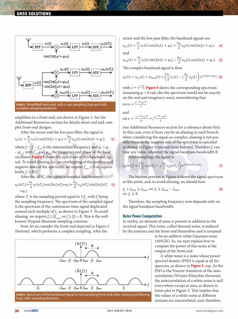
Let us first consider the front-end depicted in Figure 2 (top), which per-forms real sampling. This is a very simplified representation, but enough for our discussion. This front-end is composed of:• a bandpass filter (BPF) for image-

rejection• a mixer to bring the signal to a

lower frequency• a low pass filter (LPF) for anti-alias-

ing (aliasing is explained next); this filter can also be a bandpass filter

• an analog-to-digital converter(ADC)Of course, there are also a few

GNSS Solutions is a regular column featuring questions and answers about technical aspects of GNSS. Readers are invited to send their questions to the columnist, Dr. Mark Petovello, Department of Geomatics Engineering, University of Calgary, who will find experts to answer them. His e-mail address can be found with his biography below.

GNSS SOLUTIONS

MARK PETOVELLO is a Professor in the Department of Geomatics Engineering at the University of Calgary. He has been actively involved in many aspects of positioning

and navigation since 1997 including GNSS algorithm development, inertial navigation, sensor integration, and software development. Email: mark.petovello@ucalgary.ca

How does one compute the noise power to simulate real and complex GNSS signals?

FIGURE 1 Example of incoming signal spectrum

30 InsideGNSS J U L Y / A U G U S T 2 0 1 6 www.insidegnss.com

GNSS SOLUTIONS

amplifiers in a front-end, not shown in Figure 2. See theAdditional Resources section for details about real and com-plex front-end designs.

After the mixer and the low pass filter, the signal is

where fi = fr – fLO is the intermediate frequency and φi = φr– φLO, with fLO and φLO the frequency and phase of the local oscillator. Figure 3 shows the spectrum of this baseband sig-nal. To avoid aliasing, i.e., an overlapping of the positive and negative sides of the spectrum, we require fmin ≥ 0 or, equiva-lently, fi ≥ B/2.

After the ADC, the signal is sampled and becomes

where Ts is the sampling period equal to 1/fs, with fs being the sampling frequency. The spectrum of the sampled signal is the spectrum of the continuous-time signal duplicated around each multiple of fs, as shown in Figure 3. To avoidaliasing, we require fs ≥ 2fmax, or fs ≥ 2fi + B. This is the well-known Nyquist-Shannon sampling criterion.

Now, let us consider the front-end depicted in Figure 2(bottom), which performs a complex sampling. After the

mixer and the low pass filter, the baseband signals are

and

The complex baseband signal is then

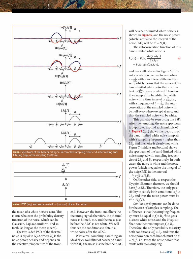
with Figure 4 shows the corresponding spectrum (assuming φ = 0 rad, else the spectrum would not be exactly on the real and imaginary axes), remembering that

and

(see Additional Resources section for a reference about this). In this case, even if there can be an aliasing in each branch, when considering the signal as complex, aliasing is not pos-sible because the negative side of the spectrum is canceled as shown in Figure 4 (second from bottom).Therefore fi can take any value, whatever the signal bandpass bandwidth B.

After sampling, the signal is

The bottom portion of Figure 4 shows the signal spectrumat this point, and, to avoid aliasing, we should have

Therefore, the sampling frequency now depends only on the signal bandpass bandwidth.

Noise Power ComputationIn reality, an element of noise is present in addition to the received signal. This noise, called thermal noise, is induced by the antenna and the front-end themselves and is assumed

to be an additive white Gaussian noise (AWGN). So, we next explain how to compute the power of this noise at the output of the front-end.

A white noise is a noise whose power spectral density (PSD) is equal at all fre-quencies, as shown in Figure 5, top. As the PSD is the Fourier transform of the auto-correlation (Wiener-Khinchin theorem), the autocorrelation of a white noise is null everywhere except at zero, as shown in lower plot in Figure 5.This implies thatthe values of a white noise at different instants are uncorrelated, and, therefore,

FIGURE 2 Simplified front-end, with a real sampling (top) and with complex sampling (bottom)

FIGURE 3 Spectrum of the baseband signal in real sampling front-end, after mixing and filtering (top), after sampling (bottom).

www.insidegnss.com J U L Y / A U G U S T 2 0 1 6 InsideGNSS 31

the mean of a white noise is zero. This is true whatever the probability density function of the noise, which can be Gaussian, Laplace, uniform, and so forth (as long as the mean is zero).

The two-sided PSD of the thermal noise is equal to N0/2, where N0 is the noise power density and depends on the effective temperature of the front-

end. However, the front-end filters the incoming signal; therefore, the thermal noise is filtered, too, and the noise just before the ADC is not white. We will thus see the conditions to obtain a white noise after the ADC.

With a real sampling, assuming an ideal brick wall filter of baseband band-width BF, the noise just before the ADC

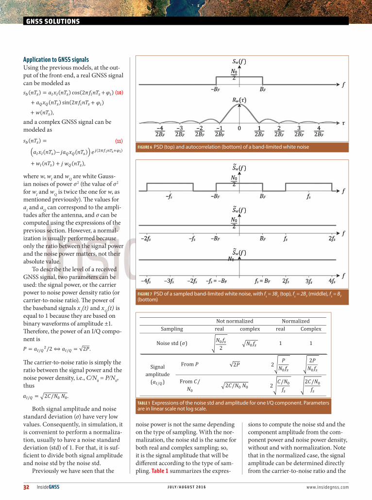
will be a band-limited white noise, as shown in Figure 6, and the noise power (which is equal to the integral of the noise PSD) will be σ2 = N0BF.

The autocorrelation function of this band-limited white noise is

and is also illustrated in Figure 6.Thisautocorrelation is equal to zero when

with k an integer different than zero, which means that the values of the band-limited white noise that are dis-tant by are uncorrelated. Therefore, if we sample this band-limited white noise with a time interval of , i.e., with a frequency of fs = , the auto-correlation of the sampled noise will be null everywhere except at zero, and thus the sampled noise will be white.

This can also be seen using the PSD. After the sampling, the noise spectrum is duplicated around each multiple of fs. Figure 7 (top) shows the spectrum of the band-limited white noise sampled with a sampling frequency higher than 2BF, and the noise is clearly not white. Figure 7 (middle and bottom) showsthe spectrum of the band-limited white noise sampled with sampling frequen-cies of 2BF and BF, respectively. In both cases, the noise is white and the noise power (which is equal to the integral of the noise PSD in the interval

) is N0BF.On the other side, to respect the

Nyquist-Shannon theorem, we should have fs ≥ 2BF. Therefore, the only pos-sibility to satisfy both conditions is fs ≥ 2BF, and thus the noise power must be σ2 = N0fs/2.

Similar developments can be done for the case of complex sampling. The difference is that the sampling frequen-cy must be equal to fs = BF /k to get a discrete white noise, and the Nyquist-Shannon theorem imposes fs ≥ BF. Therefore, the only possibility to satisfy both conditions is fs = BF, and thus the noise power on each branch must be σ2

= N0 fs, i.e., twice the noise power that exists with real sampling.

FIGURE 4 Spectrum of the baseband signal in complex sampling front-end, after mixing and filtering (top), after sampling (bottom).

FIGURE 5 PSD (top) and autocorrelation (bottom) of a white noise

32 InsideGNSS J U L Y / A U G U S T 2 0 1 6 www.insidegnss.com

GNSS SOLUTIONS

Application to GNSS signalsUsing the previous models, at the out-put of the front-end, a real GNSS signal can be modeled as

and a complex GNSS signal can be modeled as

where w, wI and wQ are white Gauss-ian noises of power σ2 (the value of σ2

for wI and wQ is twice the one for w, as mentioned previously). The values for aI and aQ can correspond to the ampli-tudes after the antenna, and σ can be computed using the expressions of the previous section. However, a normal-ization is usually performed because only the ratio between the signal power and the noise power matters, not their absolute value.

To describe the level of a received GNSS signal, two parameters can be used: the signal power, or the carrier power to noise power density ratio (or carrier-to-noise ratio). The power of the baseband signals xI(t) and xQ(t) is equal to 1 because they are based on binary waveforms of amplitude ±1. Therefore, the power of an I/Q compo-nent is

The carrier-to-noise ratio is simply the ratio between the signal power and the noise power density, i.e., C/N0 = P/N0, thus

Both signal amplitude and noisestandard deviation (σ) have very low values. Consequently, in simulation, it is convenient to perform a normaliza-tion, usually to have a noise standard deviation (std) of 1. For that, it is suf-ficient to divide both signal amplitude and noise std by the noise std.

Previously we have seen that the

noise power is not the same depending on the type of sampling. With the nor-malization, the noise std is the same for both real and complex sampling; so, it is the signal amplitude that will be different according to the type of sam-pling. Table 1 summarizes the expres-

sions to compute the noise std and the component amplitude from the com-ponent power and noise power density, without and with normalization. Note that in the normalized case, the signal amplitude can be determined directly from the carrier-to-noise ratio and the

FIGURE 6 PSD (top) and autocorrelation (bottom) of a band-limited white noise

FIGURE 7 PSD of a sampled band-limited white noise, with fs = 3BF (top), fs = 2BF (middle), fs = BF (bottom)

TABLE 1 Expressions of the noise std and amplitude for one I/Q component. Parameters are in linear scale not log scale.

www.insidegnss.com J U L Y / A U G U S T 2 0 1 6 InsideGNSS 33

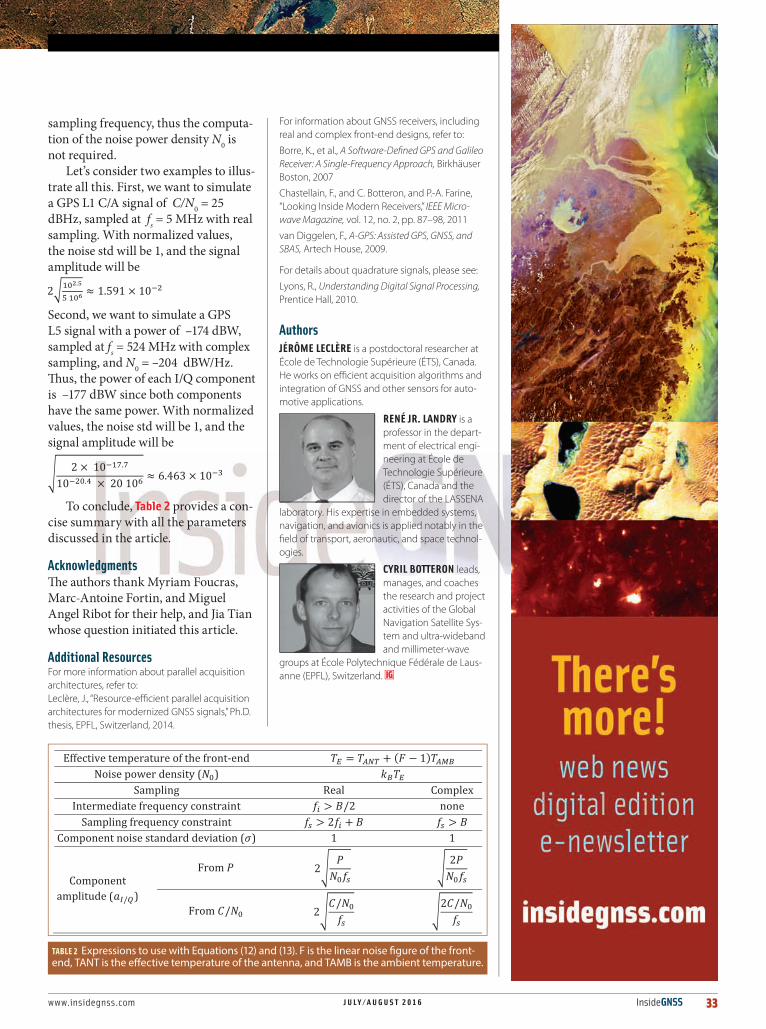
sampling frequency, thus the computa-tion of the noise power density N0 is not required.

Let’s consider two examples to illus-trate all this. First, we want to simulatea GPS L1 C/A signal of  C/N0 = 25dBHz, sampled at fs = 5MHz with realsampling. With normalized values, the noise std will be 1, and the signal amplitude will be

Second, we want to simulate a GPS L5 signal with a power of  –174 dBW,sampled at fs = 524 MHz with complexsampling, and N0 = –204  dBW/Hz.Thus, the power of each I/Q component is  –177 dBW since both componentshave the same power. With normalized values, the noise std will be 1, and the signal amplitude will be

To conclude, Table 2 provides a con-cise summary with all the parameters discussed in the article.

AcknowledgmentsThe authors thankMyriam Foucras,Marc-Antoine Fortin, andMiguelAngel Ribot for their help, and Jia Tian whose question initiated this article.

Additional ResourcesFor more information about parallel acquisition architectures, refer to:Leclère, J., “Resource-efficient parallel acquisition architectures for modernized GNSS signals,” Ph.D. thesis, EPFL, Switzerland, 2014.

For information about GNSS receivers, including real and complex front-end designs, refer to:

Borre, K., et al., A Software-Defined GPS and Galileo Receiver: A Single-Frequency Approach, Birkhäuser Boston, 2007

Chastellain, F., and C. Botteron, and P.-A. Farine, “Looking Inside Modern Receivers,” IEEE Micro-wave Magazine, vol. 12, no. 2, pp. 87–98, 2011

van Diggelen, F., A-GPS: Assisted GPS, GNSS, and SBAS, Artech House, 2009.

For details about quadrature signals, please see:

Lyons, R., Understanding Digital Signal Processing, Prentice Hall, 2010.

AuthorsJÉRÔME LECLÈRE is a postdoctoral researcher at École de Technologie Supérieure (ÉTS), Canada. He works on efficient acquisition algorithms and integration of GNSS and other sensors for auto-motive applications.

RENÉ JR. LANDRY is a professor in the depart-ment of electrical engi-neering at École de Technologie Supérieure (ÉTS), Canada and the director of the LASSENA

laboratory. His expertise in embedded systems, navigation, and avionics is applied notably in the field of transport, aeronautic, and space technol-ogies.

CYRIL BOTTERON leads, manages, and coaches the research and project activities of the Global Navigation Satellite Sys-tem and ultra-wideband and millimeter-wave

groups at École Polytechnique Fédérale de Laus-anne (EPFL), Switzerland.

TABLE 2 Expressions to use with Equations (12) and (13). F is the linear noise figure of the front-end, TANT is the effective temperature of the antenna, and TAMB is the ambient temperature.