ORIGINAL RESEARCH Open Access

How do fire behavior and fuelconsumption vary between dormant andearly growing season prescribed burns inthe southern Appalachian Mountains?Matthew C. Vaughan1 , Donald L. Hagan2* , William C. Bridges Jr3, Matthew B. Dickinson4 and T. Adam Coates5

Abstract

Background: Despite the widespread use of prescribed fire throughout much of the southeastern USA, temporalconsiderations of fire behavior and its effects often remain unclear. Opportunities to burn within prescriptivemeteorological windows vary seasonally and along biogeographical gradients, particularly in mountainous terrainwhere topography can alter fire behavior. Managers often seek to expand the number of burn days available toaccomplish their management objectives, such as hazardous fuel reduction, control of less desired vegetation, andwildlife habitat establishment and maintenance. For this study, we compared prescribed burns conducted in thedormant and early growing seasons in the southern Appalachian Mountains to evaluate how burn outcomes maybe affected by environmental factors related to season of burn. The early growing season was defined as thenarrow phenological window between bud break and full leaf-out. Proportion of plot area burned, surface fuelconsumption, and time-integrated thermocouple heating were quantified and evaluated to determine potentialrelationships with fuel moisture and topographic and meteorological variables.

Results: Our results suggested that both time-integrated thermocouple heating and its variability were greater inearly growing season burns than in dormant season burns. These differences were noted even though fuelconsumption did not vary by season of burn. The variability of litter consumption and woody fuelbed heightreduction were greater in dormant season burns than in early growing season burns. Warmer air temperatures andlower fuel moisture, interacting with topography, likely contributed to these seasonal differences and resulted inmore burn coverage in early growing season burns than in dormant season burns.

Conclusions: Dormant season and early growing season burns in southern Appalachian forests consumed similaramounts of fuel where fire spread. Notwithstanding, warmer conditions in early growing season burns are likely toresult in fire spread to parts of the landscape left unburnt in dormant season burns. We conclude that earlygrowing season burns may offer a viable option for furthering the pace and scale of prescribed fire to achievemanagement objectives.

Keywords: Fire weather, Fuel moisture, Time-integrated heating, Litter, Duff, Woody fuels, Topography

© The Author(s). 2021 Open Access This article is licensed under a Creative Commons Attribution 4.0 International License,which permits use, sharing, adaptation, distribution and reproduction in any medium or format, as long as you giveappropriate credit to the original author(s) and the source, provide a link to the Creative Commons licence, and indicate ifchanges were made. The images or other third party material in this article are included in the article's Creative Commonslicence, unless indicated otherwise in a credit line to the material. If material is not included in the article's Creative Commonslicence and your intended use is not permitted by statutory regulation or exceeds the permitted use, you will need to obtainpermission directly from the copyright holder. To view a copy of this licence, visit http://creativecommons.org/licenses/by/4.0/.

* Correspondence: dhagan@clemson.edu2Department of Forestry and Environmental Conservation, ClemsonUniversity, 202 Lehotsky Hall, Clemson, SC 29634, USAFull list of author information is available at the end of the article

Fire EcologyVaughan et al. Fire Ecology (2021) 17:27 https://doi.org/10.1186/s42408-021-00108-1

Resumen

Antecedentes: A pesar del uso generalizado de las quemas prescriptas a través de muchas zonas del sureste de losEEUU, las consideraciones temporales sobre el comportamiento del fuego y sus efectos todavía permanecen pococlaras. La oportunidad de quemar dentro de ventanas de prescripción meteorológica varía estacionalmente y a lolargo de gradientes biogeográficos, particularmente en terrenos montañosos donde la topografía puede alterar elcomportamiento del fuego. Los gestores frecuentemente buscan expandir el número de días disponibles paraquemar para cumplir con sus objetivos de manejo, como la reducción de combustibles peligrosos, el control de lavegetación no deseada, y el establecimiento y mantenimiento del hábitat para la fauna. Para este estudio,comparamos las quemas prescriptas conducidas en la estación de dormición y en la de crecimiento temprano enlas Montañas Apalaches del sur para evaluar como los resultados de las quemas pueden ser afectados por laestación de quema. La estación de crecimiento temprano fue definida como la angosta ventana fenológica entre elrompimiento del crecimiento de los meristemas de crecimiento y la aparición de las hojas. La proporción de laparcela quemada, el consumo de combustible superficial, y la integral entre el tiempo y el calor recibido medidocon termocuplas fueron cuantificados y evaluados para determinar relaciones potenciales con la humedad elcombustible y variables topográficas y meteorológicas.

Resultados: Nuestros resultados sugieren que tanto la integral entre tiempo y el calor recibido por la termocupla ysu variabilidad fueron mayores en las quemas al inicio de la temporada de crecimiento que en las quemas enestado de dormición. Esas diferencias fueron notables aún cuando el combustible consumido no varió entreestaciones de quemas. La variabilidad en el consumo de broza y la reducción de la carga superficial de combustiblede leñosas fueron mayores en la estación de dormición que en las quemas al inicio de la estación de crecimiento.Las temperaturas del aire más cálidas y la menor humedad del combustible, interactuando con la topografía,probablemente contribuyeron a esas diferencias estacionales y resultaron en mayores coberturas de quema in lasquemas realizadas en la estación de crecimiento que en la estación de dormición.

Conclusiones: Las quemas prescriptas realizadas tanto durante la dormición como al inicio de la estación decrecimiento en las montañas Apalaches del Sur consumieron similares cantidades de combustible con el avancedel fuego. A pesar de ello, las condiciones más cálidas en la estación de crecimiento temprano parecen resultar enla propagación del fuego a partes del paisaje que quedaban sin quemar en quemas realizadas durante ladormición. Concluimos que las quemas prescriptas al inicio de la estación de crecimiento pueden ofrecer unaopción viable para avanzar en ritmos y escalas de quemas prescriptas para alcanzar objetivos de manejo.

Palabras clave: Meteorología de fuegos, Humedad del Combustible, Integral tiempo-temperatura, broza, mantillo,combustibles leñosos, topografía

BackgroundFire is firmly embedded in the natural history and hu-man experience of the American Southeast. Evidencesuggests that fire has been prevalent in the Southeast formillennia, from the written accounts of explorers whodescribed pervasive smoke and open woodlands (Fowlerand Konopik 2007), to reconstructions of past fire occur-rence using physical measurements synthesized by re-searchers (Delcourt and Delcourt 1998; Lafon et al.2017). Humans before and after Euro-American settle-ment in the 1700s and 1800s used fire to cultivate habi-tat for their livelihood (Owsley 1949; Stewart 2002;Abrams and Nowacki 2008), fostering a culture of burn-ing that may inform our present treatment of fire. Rec-ognizing that decades of fire suppression in the 1900soften led to hazardous fuel accumulation and forest“mesophication” (Nowacki and Abrams 2008), policy-makers and land managers have increasingly endorsedand implemented prescribed fire in recent decades to

reduce wildfire risk and promote ecosystem health andresiliency (Pyne 1982; Rothman 2007; Waldrop andGoodrick 2012). Today, more area is treated with pre-scribed fire on an annual basis in the Southeast than inany other region of North America (Wade et al. 2000;Kobziar et al. 2015; Melvin 2018).Wildland fire is thought to have occurred more often

in different seasons prior to fire suppression than it doestoday, particularly in the Southeast’s most fire-prone en-vironments (Komarek 1965, 1974; Lafon 2010). Habitatsfavorable to forage and harvest could have been main-tained by humans burning in a variety of seasons(Eldredge 1911; Jurgelski 2008). Historically, lightning ig-nitions may have occurred in drier fuels under moreopen canopies, a potential source of fire following springand summer thunderstorms (Barden and Woods 1974;Cohen et al. 2007). Lightning-ignited fires in the south-ern Appalachians were unlikely to have been common,however, and wet weather would typically constrain their

Vaughan et al. Fire Ecology (2021) 17:27 Page 2 of 16

spread (Lafon et al. 2017). Wildland fire extent in largelydeciduous forests of the southern Appalachians today isinversely related to vegetation greenness (Haines et al.1975; Norman et al. 2019), with most area burned eitherin late winter (dormant season) and spring beforecomplete leaf expansion (early growing season) or in thefall following leaf abscission (Schroeder and Buck 1970).Fire seasonality is further confounded in mountainoustopography with less predictable fire behavior due tomore heterogeneous temperature and moisture condi-tions across the landscape (Stambaugh and Guyette2008; Lesser and Fridley 2016).The use of prescribed fire has expanded substantially

in the southern Appalachians in recent decades amidwidespread efforts to reduce hazardous fuel loads, re-store woodland and savannah communities, and increasenative oak (Quercus L.) and yellow pine (Pinus L.) regen-eration (Van Lear and Waldrop 1989; Waldrop andBrose 1999; Brose et al. 2001). Using fire for these objec-tives has largely occurred in the dormant season beforesubstantial spring green-up, mirroring prescriptive pat-terns of fire use in the Southeast more broadly (VanLear and Waldrop 1989; Wade and Lunsford 1989).Burning in the dormant season as opposed to the grow-ing season may decrease the risk of fire escape, particu-larly in mid-late winter with lower ambient temperaturesand more predictable wind patterns (Mobley and Balmer1981; Wade and Lunsford 1989; Robbins and Myers1992). Spring burning has also been less favored due topotential detrimental effects on wildlife species that maybe more vulnerable to fire during that stage of their lifehistory (Landers 1981; Cox and Widener 2008). In lightof the prevalence of dormant season burning, potentialgrowing season fire behavior and effects are not wellunderstood (Knapp et al. 2009; Reilly et al. 2012). How-ever, there is likely a window in the early growing seasonwhen dry forest floor conditions permit the combustionof fuels and spread of fire – perhaps to a greater extentthan would occur under typical dormant season burningconditions. For managers in the southern Appalachianswho want to expand their prescribed fire programs,growing season burning could offer an alternative todormant season burning, allowing for increased oppor-tunities to burn. Evidence of historical fire regimes sug-gests fire occurrence outside of the dormant season(Lafon et al. 2017; Stambaugh et al. 2018). It remains tobe seen, however, how growing season burns compare todormant season burns for accomplishing managementobjectives of reducing fuel loads and restoring habitats.Improved knowledge of how and why fire behavior

and first-order fire effects vary seasonally may improvesouthern Appalachian forest management. Variability inmeteorological and topographic factors influencing firebehavior may suggest the extent to which prescribed fire

would be effective in achieving fuel load reduction, afirst-order fire effect (Reinhardt and Keane 2009; Kreyeet al. 2020). Solar radiation drives the magnitude and ex-tent of surface fuel drying and thereby influences fire be-havior relative to latitude, slope, and aspect (Byram andJemison 1943). Slope position further influences the leveland duration of heating from fire along moisture gradi-ents from sheltered coves to prominent peaks across amountainous landscape (Reilly et al. 2012; Dickinsonet al. 2016). The effects of topography on fire behaviorand resulting fuel consumption may also be reinforcedor overridden by changing weather patterns over pheno-logical transitions (Norman et al. 2017). Upon longerand warmer spring days, aboveground perennial emer-gence and heightened plant transpiration may lead togreater variability in the distribution of live fuel moisture(Jolly and Johnson 2018). In autumn, surface windsunder an open canopy following leaf fall may compoundmoisture loss on upper slopes and ridges, creating a fuelbed more conducive to high rates of fire spread (Dickin-son et al. 2016; Kreye et al. 2020). Fuel moisture altersflammability and may suggest fine-scale differences infire effects (Sparks et al. 2002; Slocum et al. 2003; Kreyeet al. 2018).

Research questionsFor this study, we compared seven prescribed burnsconducted in the dormant and early growing seasons inthe southern Appalachians to evaluate season of burn ef-fects on fire behavior and fuel consumption. In situ, rep-resentative ex situ, and digital elevation model (DEM)-derived data were used to address the followingquestions:

1. How do meteorological conditions influencingsurface fuel moisture and proportion of plot areaburned vary by season of burn?

2. How do time-integrated thermocouple heating, sur-face fuel consumption, and the relationship betweenthese variables differ by season of burn?

3. How are slope position and solar heat load relatedto fire behavior in dormant and early growingseason burns?

For Question #1, we hypothesized that diurnal solarradiation and average ambient temperatures would behigher in the early growing season, resulting in lowersurface fuel moisture and a greater proportion of treat-ment area burned than in the dormant season. ForQuestion #2, we hypothesized that the degree and vari-ability of time-integrated heating would be greater inearly growing season burns than in dormant seasonburns. We also hypothesized that the degree and vari-ability of litter and fine woody fuel consumption would

Vaughan et al. Fire Ecology (2021) 17:27 Page 3 of 16

be greater in early growing season burns, driven by vari-ations in fuel moisture. Furthermore, we expected thatlitter and duff consumption would rise at a greater ratewith increasing time-integrated heating (have a steeperslope between these variables) in dormant season burnsthan in early growing season burns. For Question #3, wehypothesized that bole char height would rise at agreater rate with both increasing slope position and in-creasing solar heat load (have steeper slopes betweenthese pairs of variables) in dormant season burns than inearly growing season burns. Furthermore, we expectedthat bole char height would be more strongly correlatedwith both slope position and solar heat load in dormantseason burns than in early growing season burns.

MethodsStudy areaThis study was conducted along the southern Blue RidgeEscarpment of the Appalachian Mountains in the

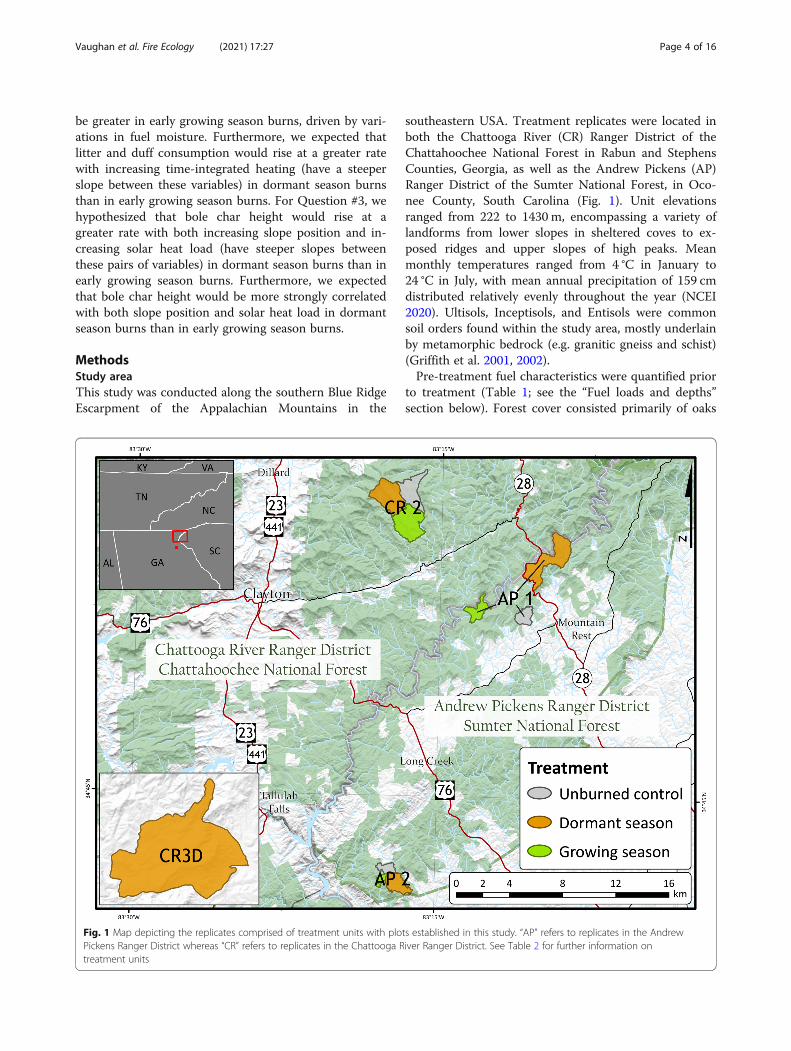
southeastern USA. Treatment replicates were located inboth the Chattooga River (CR) Ranger District of theChattahoochee National Forest in Rabun and StephensCounties, Georgia, as well as the Andrew Pickens (AP)Ranger District of the Sumter National Forest, in Oco-nee County, South Carolina (Fig. 1). Unit elevationsranged from 222 to 1430 m, encompassing a variety oflandforms from lower slopes in sheltered coves to ex-posed ridges and upper slopes of high peaks. Meanmonthly temperatures ranged from 4 °C in January to24 °C in July, with mean annual precipitation of 159 cmdistributed relatively evenly throughout the year (NCEI2020). Ultisols, Inceptisols, and Entisols were commonsoil orders found within the study area, mostly underlainby metamorphic bedrock (e.g. granitic gneiss and schist)(Griffith et al. 2001, 2002).Pre-treatment fuel characteristics were quantified prior

to treatment (Table 1; see the “Fuel loads and depths”section below). Forest cover consisted primarily of oaks

Fig. 1 Map depicting the replicates comprised of treatment units with plots established in this study. “AP” refers to replicates in the AndrewPickens Ranger District whereas “CR” refers to replicates in the Chattooga River Ranger District. See Table 2 for further information ontreatment units

Vaughan et al. Fire Ecology (2021) 17:27 Page 4 of 16

(Quercus L.), hickories (Carya L.), and pines (Pinus L.)across the following ecozones (Simon et al. 2005; Simon2015): Dry-Mesic Oak-Hickory Forest, Shortleaf Pine-Oak Forest and Woodland, Mixed Oak/RhododendronForest, and Montane Oak-Hickory Forest. Substantialmidstory encroachment was present from mesophytichardwoods [e.g., red maple (Acer rubrum L.)], mountainlaurel (Kalmia latifolia L.), and great rhododendron(Rhododendron maximum L.).

Study designThe study was established as a randomized completeblock design, with treatments of dormant season burn

(d), growing season burn (g), and an unburned control(c) replicated (blocked) three times. A fourth, standa-lone, dormant season burn in a planned, additional repli-cate was also included to equal a total of 10 treatmentunits. Treatment units ranged in area from 43 to 567 ha,with a mean area of 293 ha (Table 2). Twenty plots werestratified across a variety of slope, aspect, and landscapepositions within each treatment unit (except for 5 plotsin the standalone unit). This yielded 180 plots with us-able data that were included in analyses, with 5 plots inburn treatment units lost due to construction of controllines which contained different areas than had been an-ticipated. Each plot was 30 m × 30m (900 m2),

Table 1 Summary of pre-treatment fuel characteristics between designated treatments across all study plots

Woody fuel characteristic (Brown 1974) Designated treatment Mean (± SE) Overall mean (± SE)

Litter load[kg ha−1]

C 6707.2 (± 330.2) 6684.4 (± 179.7)

DS 6876.7 (± 292.2)

GS 6453.1 (± 315.4)

Woody fuelbed height[cm]

C 13.0 (± 1.2) 14.1 (± 0.7)

DS 14.7 (± 1.3)

GS 14.6 (± 1.1)

1-h woody load[kg ha−1]

C 551.1 (± 26.8) 604.4 (± 19.8)

DS 619.1 (± 32.1)

GS 642.0 (± 41.8)

10-h woody load[kg ha−1]

C 1662.0 (± 127.2) 1881.7 (± 90.9)

DS 2191.3 (± 174.2)

GS 1765.9 (± 157.7)

100-h woody load[kg ha−1]

C 3493.8 (± 390.0) 4941.0 (± 421.0)

DS 6355.4 (± 1,014.9)

GS 4856.0 (± 519.4)

1000-h woody load[kg ha−1]

C 6356.4 (± 1,189.2) 5457.6 (± 540.6)

DS 5480.3 (± 887.6)

GS 4534.0 (± 665.0)

Table 2 Listing of treatment units used in this study by replicate and corresponding treatment, with area, date of burn (ifapplicable), and elevation range. Firing methods included both hand ignition and remote aerial ignition, with a spot fire techniqueused for hand ignitions when possible to simulate aerial ignition

Replicate Treatment Unit Area (ha) Date of burn Elevation range (m)

AP 1 Unburned control (C) AP1C 133.8 n/a 498–625

Dormant season burn (DS) AP1D 538.1 01/31/18 480–772

Growing season burn (GS) AP1G 160.5 04/18/18 454–560

AP 2 Unburned control (C) AP2C 80.8 n/a 360–470

Dormant season burn (DS) AP2D 205.3 03/18/19 275–468

Growing season burn (GS) AP2G 43.3 04/21/18 312–462

CR 2 Unburned control (C) CR2C 323.2 n/a 704–1157

Dormant season burn (DS) CR2D 441.5 04/05/18 724–1430

Growing season burn (GS) CR2G 435.3 04/24/19 622–963

CR 3 Dormant season burn (DS) CR3D 566.5 03/03/18 222–386

Vaughan et al. Fire Ecology (2021) 17:27 Page 5 of 16

subdivided into nine 10m × 10m (100 m2) subplots de-lineated by 16 grid point intersections and oriented withouter boundaries running magnetic north (0°) and east(90°) from its point of origin (Fig. 2). Surface fuel tran-sects (15.24 m in length) were superimposed on eachplot, separated by 20° magnetic azimuth emanating fromthe plot origin.Prescribed burns were implemented by US Forest

Service fire practitioners as a part of official burn plansand coordinated with Clemson University for purposesof this study. Dormant season burns were defined asthose occurring after autumn leaf-fall and before springgreen-up (typically before last frost), whereas growingseason burns were considered as those occurring in theearly spring green-up period (typically after last frost)before complete overstory leaf-out. At the elevations ofthe study area, green-up typically begins in early April,with full leaf-out occurring by May. Burn treatmentsoccurred between January 31–April 5 (dormant season)and April 18–24 (growing season) in 2018 and 2019(Table 2). Firing methods included hand ignition usingdrip torches as well as remote aerial ignition using de-layed aerial ignition devices launched from a helicopteron some burns. A spot fire technique was used for handignitions when possible in order to simulate aerialignitions.

Field sampling and data preparationFuels were measured before and after each burn to de-termine changes in surface fuel load across all plots.Complementary measurements of litter and duff con-sumption were taken at a greater sampling density in asubset of plots (see “Fuel loads and depths” sectionbelow). Fuel moisture was sampled the morning of burnsand levels of heating were recorded throughout eachburn day in situ in the same subset of “fire behaviorplots.” Measurements of bole char height were taken inall plots following each burn. Visual evidence of thepresence or absence of fire (y/n) was noted at grid pointintersections, with a 50% threshold of grid points indi-cating the presence of fire used to qualify burn treat-ments for plot-level variables. The proportion of plotarea burned was calculated by dividing the number ofgrid points with evidence of charred material by the totalnumber of grid point intersections within a plot.

Fuel loads and depthsFuel measurements of woody fuelbed height and finewoody debris counts (1-h, 10-h, and 100-h) were takenin the growing season pre- and post-burn using a modi-fied version of Brown’s Planar Intercept Method (Brown1974; Stottlemyer 2004; Coates et al. 2019). This methodwas utilized in all plots within the treatment units (3

Fig. 2 Representative diagram indicating the layout, orientation, and dimensions of each plot with interior grid point intersections. The (x, y)Cartesian coordinate pairs for each grid point represent the longitudinal (x) and latitudinal (y) distance from the origin

Vaughan et al. Fire Ecology (2021) 17:27 Page 6 of 16

transects per plot; n = 60 measurement units per treat-ment unit), which included measurements taken at des-ignated intervals along transects emanating from theplot origin (3.66 m, 7.62 m, and 12.19 m). Slope valueswere derived from a digital elevation model along linesrepresenting the length and orientation of each transectin a geographic information system (Esri 2019). Mea-surements of litter and duff consumption were taken atgrid point intersections within a subset of 5 fire behaviorplots per burn treatment (16 litter and 16 duff nails perplot; n = 80 measurement units for each fuel class pertreatment unit) using depth reduction measurements on30 cm nails. Nails for this purpose were driven into theground prior to ignition so that the heads were at thesame pre-burn height as the fuel class being measured.Post-burn fuel height was marked on the nail within 24h after burn completion to determine changes in litterand duff depth. All fuel depth and height measurementswere recorded to the nearest 0.64 cm.Raw fuel measurements were used to estimate fuel

weight per area (load) for each fuel class, calculated byplot (Brown’s protocol) or grid point (nail method). Fuelconsumption was used as the metric of response. Theaverage change in fuel height or load for each fuel classin unburned control units was subtracted from thechange in fuel height or load in corresponding burntreatments in the same replicate to account for fuelchanges in the absence of fire. Bulk density, quadraticmean diameter, specific gravity, and non-horizontal cor-rection coefficients were chosen from representativevalues for the region and forest type (Ottmar andAndreu 2007; B. Buchanan, United States Forest Service,Roanoke, VA, USA, unpublished report). The degreeand variability of surface fuel consumption as quantifiedby changes in woody fuelbed height (cm); 1-h, 10-h, and100-h woody fuel load (kg ha−1); and litter and duff load(kg ha−1) were compared between dormant and growingseason burn treatments.

Fuel moistureFuel moisture was measured in situ for litter and 1-hwoody (pooled) as well as 10-h woody fuels in the firebehavior plots on the day of burn prior to ignition. Grabsamples for this purpose (approx. 20 g) were collectedfrom each plot corner and center (origin/SW, NW, NE,SE, and center), with disturbance of the surface fuel bedminimized at sampling locations [(5) litter/1-h woodyand (5) 10-h woody fuel samples per plot; n = 25 meas-urement units for each fuel class per treatment unit]. Allsamples were sealed in 946 mL bags and weighed in thelab upon unsealing (wet mass), dried to constant weightat 75 °C (48 h), and re-weighed after drying (dry mass).Fuel weight measurements for this purpose were re-corded to the nearest 0.01 g. Relative moisture content

for these fuels (%) was calculated using the formulawet mass−dry mass

dry mass � 100 (Cannon and Parkinson 2019) and

averaged by plot. Moisture content for coarser fuels andduff was not measured, as these materials are generallynot consumed under typical prescribed fire conditions inthe region.

Fire behaviorTemperature was recorded continuously in situ before,during, and after passage of flaming fronts on each burnday using thermocouple probes. Onset Computer Cor-poration (Bourne, MA, USA) HOBO Type K Thermo-couple data loggers were programmed to logtemperature at a 1-s interval throughout the burn day(recording period 9 h 1min 58 s), which were then at-tached to Cole-Parmer Instrument Company Digi-SenseType K thermocouple probes (Vernon Hills, IL, USA),packaged, and buried in the ground approximately 15cm deep prior to ignition. Probes protruded above-ground (sheath length = 30.48 cm) and were orientedsuch that the tip (sheath diameter = 0.1016 cm) faceddownward at a uniform height of 2.54-5.08 cm above thelitter surface (Fig. 3). Thermocouples were positioned torecord temperatures at each grid point intersectionwithin the subset of 5 fire behavior plots per unit coinci-dent with nail measurements of litter and duff consump-tion (16 probes per plot; n = 80 measurement units pertreatment unit). Data logger and probe packages wereretrieved within 48 h after deployment with temperaturemeasurements subsequently downloaded from each de-vice. Data from loggers showing abnormal temperatureprofiles uncharacteristic of passage of a flaming front(i.e., suggesting recording failure) were excluded fromanalyses.Metrics of fire behavior were derived from thermo-

couple temperature profiles, calculated via different ap-proaches and thresholds using an automated script inMATLAB R2020a Update 5 (MathWorks 2020). Follow-ing initial comparisons of these metrics, the time integralof absolute temperature above 60 °C (ABS60 approach)was chosen as the representative thermocouple heatingmetric relative to fire intensity for subsequent analysis.The time integral of temperature is the Riemann sumapproximation of the product of time step andtemperature, representing both the relative degree andresidence time (i.e., “dose”) of fire-induced heating expe-rienced at a thermocouple probe tip. A threshold of60 °C was chosen as the temperature at or above whichthermocouple recordings would not only represent am-bient heating, but a level of heating reached as a resultof contact with the flaming front (Dickinson andJohnson 2004; Bova and Dickinson 2008). Temperaturethresholds were also distinguished by their relative

Vaughan et al. Fire Ecology (2021) 17:27 Page 7 of 16

sensitivity in predicting surface fuel consumption duringand after passage of a flaming front. The degree andvariability of time-integrated thermocouple heating(ABS60 approach: ∫ABS60; °C s) as well as the relation-ship between pooled litter and duff consumption (nailmethod; kg ha-1) vs. ∫ABS60 at plot grid point intersec-tions (aggregated as plot averages) were compared be-tween dormant and growing season burn treatments.Bole char height, an estimate of flame length related to

thermocouple temperatures, was measured on hardwoodtree species (e.g., Quercus spp., Acer spp., Liriodendrontulipifera) at all plot grid point intersections within burnunits (Pomp et al. 2008). Measurements of bole charheight were taken on the nearest charred bole (2.54 cmprecision) within 3.05 m of each grid point (16 pointsper plot; n = 320 measurement units per treatment unit).Plot averages were obtained from these measurements.Bole char heights likely underestimated true flamelength (Cain 1984) and were not measured on yellowpines [e.g., pitch pine (Pinus rigida Mill.) or shortleafpine (Pinus echinata Mill.)] due to the increased likeli-hood of fire spread on the bark of these trees irrespect-ive of surface flame heights.

Meteorological variablesMeteorological conditions represented by solar radiation,wind velocity, air temperature, fuel temperature, andrelative humidity (RH) were gathered ex situ from thenearest Remote Automatic Weather Station (RAWS) atsimilar elevation to each treatment unit (MesoWest2019). Weather information for each burn day was de-rived from the Andrew Pickens (Station ID: WLHS1),Tallulah (Station ID: TULG1), and Chattooga (StationID: CHGG1) stations in northwestern South Carolinaand northeastern Georgia. These weather stations werelocated within 21 km of corresponding burn locations.Solar radiation was summed and remaining variableswere averaged between 08:00 and 19:59 local time,

adjusted relative to daylight savings time clock forwarddates on March 11, 2018, and March 10, 2019 (12 mea-surements of each variable at 1-h increments on thehour). Additionally, the reported Keetch-Byram DroughtIndex (KBDI) was gathered for each corresponding burnday, accessed through the Weather Information Man-agement System (WIMS) (WIMS 2019). The degree andvariability of both meteorological conditions (RAWS/WIMS) and fuel moisture (grab samples) on burn dayswere quantified for total solar radiation (KW-h/m2), airtemperature (°C), fuel temperature (°C), wind speed (m/s), RH (%), KBDI, pooled litter and 1-hr woody fuelmoisture (%), and 10-h woody fuel moisture (%) to com-pare between dormant and growing season burntreatments.

Topographic variablesTopographic variables were derived from a digital eleva-tion model (DEM) in a geographic information system(GIS) to evaluate topographic effects on fire behavior. ADEM covering the study area was downloaded as part ofthe National Elevation Dataset from the U.S. GeologicalSurvey’s The National Map Viewer at a spatial resolutionof 1/9 arc-second and transformed to a Universal Trans-verse Mercator (UTM) Zone 17 projected coordinatesystem (3.18 m cell size) (Esri 2019). The DEM had pitsremoved using TauDEM and was clipped to the neces-sary extent for analysis in ArcGIS Desktop 10.7.1 (Tar-boton 2015; Esri 2019). Each index variable wasnormalized to a scale of 0-1 using the Raster Calculatortool and extracted using the Extract Multi Values toPoints tool (Esri 2019).Topographic Position Index (TPI) was used to quantify

slope position, based on the relative difference betweena given point’s elevation and the average elevation of itssurrounding terrain within a defined window (Guisanet al. 1999; De Reu et al. 2013). Lower values repre-sented more sheltered parts of the landscape whereas

Fig. 3 Diagram of thermocouple setup deployed at each plot grid point intersection. Data loggers were buried belowground in order to beshielded from fire temperatures aboveground. Probes attached to and extending from the data loggers were arranged with the tip at a uniformheight and orientation above the litter surface

Vaughan et al. Fire Ecology (2021) 17:27 Page 8 of 16

higher values represented greater exposure. A rectangu-lar window of 1000 m × 1000m was chosen to definethe focal area, with its average elevation subtracted fromeach cell in the DEM using the ArcGIS Geomorphome-try and Gradient Metrics Toolbox to derive TPI (Evanset al. 2014a, b; A. Evans, Texas A&M University, CollegeStation, TX, USA, personal communication; Esri 2019).Heat Load Index (HLI) was used to quantify solar radi-ation as a function of aspect, further incorporating theeffects of slope and latitude to linearize compass azi-muth such that it ranges from the lowest values onnortheast-facing slopes to the highest values onsouthwest-facing slopes (Beers et al. 1966; McCune andKeon 2002). HLI was derived from the DEM using theArcGIS Geomorphometry and Gradient Metrics Tool-box (Evans et al. 2014b; Esri 2019). TPI and HLI wereaveraged by plot area and related to bole char height (m)as topographic predictors of fire behavior, compared be-tween dormant and growing season burns by individualburns and treatment means.

Statistical analysesA statistical model was developed that related the meansof the continuous dependent variables to the treatments.Model effects included treatment (fixed), replicate (ran-dom), replicate crossed with treatment (random), and/orplot nested within treatment and replicate (random).Analysis of variance (ANOVA) techniques were used toevaluate the model terms and specifically test for treat-ment effects. For some variables, the model residuals didnot follow a normal distribution with stable varianceacross treatments, and therefore either a Kruskal-Wallisrank-based ANOVA (Boos and Brownie 1992) or a gen-eralized linear model with an exponential distributionwas used to test the treatment effect on responses.A statistical model was also developed that related re-

sponse variability to the treatments. Response variabilitywas quantified as the coefficient of variation (CV).Model effects for this model included treatment (fixed)and/or replicate (random). Either a Wilcoxon rank sumtest (Mann-Whitney U test) or a generalized linearmodel with an exponential distribution was used to testthe treatment effects on the response CVs.Ordinary least squares regression modeling was used

to estimate the slope and associated root mean squareerror (RMSE) between selected pairs of response vari-ables within each treatment unit. A log transformationwas used on heavily skewed distributions when estimat-ing the bivariate relationships. The slopes were includedin a statistical model to relate to the treatments includ-ing model effects of treatment (fixed), replicate (ran-dom), and replicate crossed with treatment (random). Aone-way ANOVA was used to test for the treatment ef-fect in this model. The RMSEs were related to

treatments with a statistical model including treatment(fixed) and replicate (random) only, also with a one-wayANOVA used to test for the treatment effect.Across all models of treatment effects, response variable

observations were aggregated at different levels with theoverall objective of producing independent observationsto be used in the model analyses. Statistical significancewas evaluated either at the α = 0.05 level (non-rankedvalues) or α = 0.10 level (ranked values). All analyses wereperformed using JMP Pro 15.1.0 and/or RStudio Desktop(up to v. 1.4.1717) within the R programming languageand software environment (up to 4.1.0) (SAS 2019; R CoreTeam 2021; RStudio 2021).

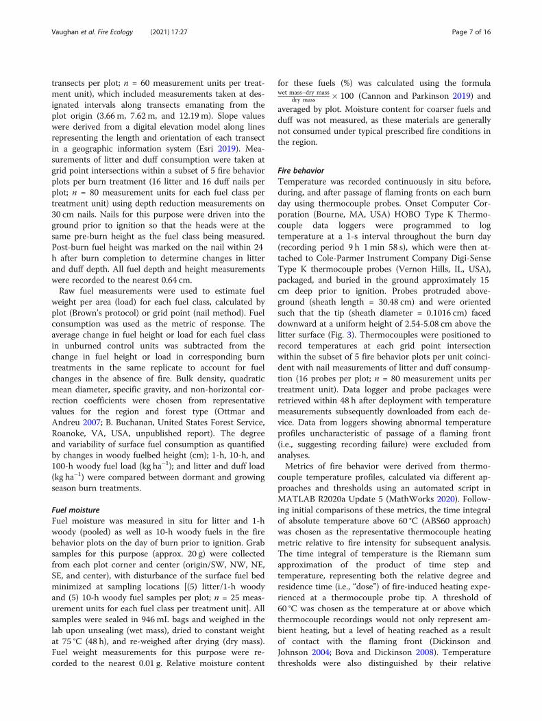
ResultsMeteorology, fuel moisture, and proportion of plot areaburnedThe early growing season was characterized by greatersolar radiation, warmer air temperatures, and warmerfuels relative to the dormant season. While air tempera-tures were cooler in the dormant season, they were morevariable. This, however, did not translate to greater vari-ation in fuel temperatures in the dormant season. Othermeteorological parameters (wind speed, relative humid-ity, KBDI) did not significantly differ between seasons.Woody fuel moisture, for both 1-h and 10-h lag classes,was greater in the dormant season – but variation in fuelmoisture did not vary between seasons (Table 3). Theproportion of plot area burned was significantly greater,and less variable, in early growing season burns than indormant season burns (Fig. 4), with burned area correl-ating with fuel moisture (Fig. 5).

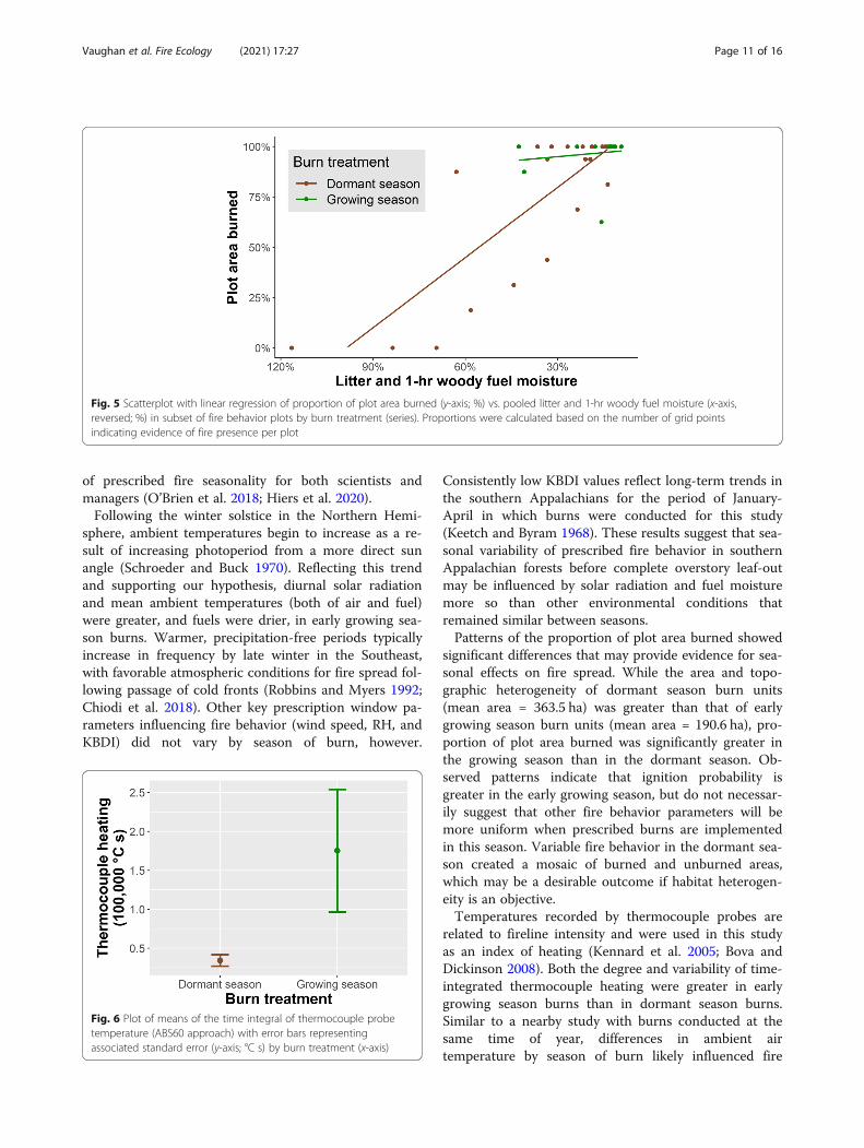
Time-integrated heating and fuel consumptionTime-integrated thermocouple heating (∫ABS60) wasmore than 5x greater in the early growing season than inthe dormant season and was also more variable (Fig. 6).This pattern was largely driven by an increase in heatingfrom fire midday and onward (Fig. 7).Woody fuelbed height; and 1-h, 10-h, and 100-h

woody fuel consumption as measured using Brown’s Pla-nar Intercept Method were not significantly different be-tween burn treatments. Likewise, using the nail method,litter consumption was not significantly different be-tween burn treatments. While mean differences werenot statistically different between treatments, there wasgreater variability in the change in woody fuelbed heightand litter consumption in dormant season burns. How-ever, duff consumption (nails) was significantly greaterin growing season burns, with no measurable duff con-sumption observed in dormant season burns (Table 4).Slope of the linear line of best fit between pooled litterand duff consumption and log-transformed ∫ABS60 didnot differ significantly between burn treatments, nor was

Vaughan et al. Fire Ecology (2021) 17:27 Page 9 of 16

there a difference in the root mean squared error(RSME) between treatments.

Topographic effects on fire behaviorHeat load index and bole char height were positivelycorrelated. While the slope of this regression was steeperin dormant season burns compared to growing seasonburns (2.2 vs. 1.4), these differences were not statisticallysignificant. Likewise, there were no statistically signifi-cant treatment effects for root mean squared errors orproportion of variance. A summary of bivariate compari-sons of bole char height vs. topographic position andheat load indices by unit and treatment can be found inFig. 8.

DiscussionThis study examined factors of the fire environment re-lated to season of burn to gain a better understanding ofhow these parameters influence prescribed fire behaviorand first-order effects. Relating fire behavior and fire ef-fects to environmental mechanisms representative ofburning season may promote meaningful interpretations

Table 3 Summary of statistical comparisons of meteorological conditions from Remote Automatic Weather Stations (RAWS) or asreported in the Weather Information Management System (WIMS) and fuel moisture collected in the field (grab samples) on burndays by variable and burn treatment. Statistical analyses were performed using a non-parametric Kruskal-Wallis rank-based standardleast squares ANOVA aggregated by plot (grab samples) or unit (RAWS/WIMS) with fixed effect of treatment and random effects ofreplicate and/or replicate crossed with treatment (response) or fixed effect of treatment and random effect of replicate (variability ofresponse). Response variables include both the mean (± standard error) and coefficient of variation (CV; %). Tests with statisticalsignificance (α = 0.10) are reported in boldface

Response variable (*α = 0.10) Burn treatment Mean (± SE) CV (%)

Meteorological conditions (RAWS/WIMS)

Total solar radiation [KW-h/m2]Mean: F1, 2.4 = 7.24, P = *0.09

DS 5.4 (± 0.8) n/a

GS 6.7 (± 0.5) n/a

Air temperature [°C]Mean: F1, 2.0 = 12.00, P = *0.07CV: F1, 3.2 = 10.07, P = *0.05

DS 10.6 (± 1.8) 48.4

GS 21.7 (± 2.3) 21.3

Fuel temperature [°C]Mean: F1, 1.8 = 36.07, P = *0.03CV: F1, 1.5 = 9.96, P = 0.12

DS 14.1 (± 2.8) 59.9

GS 26.0 (± 2.2) 32.2

Wind speed [m/s]Mean: F1, 2.4 = 0.54, P = 0.53CV: F1, 3.2 = 0.88, P = 0.41

DS 1.5 (± 0.3) 50.6

GS 1.6 (± 0.4) 34.1

Relative humidity (RH) [%]Mean: F1, 3.2 = 0.38, P = 0.58CV: F1, 2.6 = 0.07, P = 0.81

DS 27.2 (± 1.4) 49.4

GS 31.4 (± 3.1) 40.7

Keetch-Byram Drought Index (KBDI)Mean: F1, 2.8 = 2.51, P = 0.22

DS 23.8 (± 12.6) n/a

GS 61.7 (± 13.4) n/a

Fuel moisture (grab samples)

Litter and 1-h woody [%]Response: F1, 2.0 = 71.08, P = *0.01Variability: F1, 2.4 = 3.75, P = 0.17

DS 39.2 (± 6.3) 36.0

GS 17.9 (± 2.7) 27.1

10-h woody [%]Response: F1, 2.6 = 9.79, P = *0.06Variability: F1, 3.2 = 1.83, P = 0.26

DS 38.9 (± 8.0) 39.6

GS 14.6 (± 1.0) 20.9

Fig. 4 Boxplot of proportion of plot area burned (y-axis; %) by burntreatment (x-axis). Proportions were calculated based on the numberof grid points indicating evidence of fire presence per plot

Vaughan et al. Fire Ecology (2021) 17:27 Page 10 of 16

of prescribed fire seasonality for both scientists andmanagers (O’Brien et al. 2018; Hiers et al. 2020).Following the winter solstice in the Northern Hemi-

sphere, ambient temperatures begin to increase as a re-sult of increasing photoperiod from a more direct sunangle (Schroeder and Buck 1970). Reflecting this trendand supporting our hypothesis, diurnal solar radiationand mean ambient temperatures (both of air and fuel)were greater, and fuels were drier, in early growing sea-son burns. Warmer, precipitation-free periods typicallyincrease in frequency by late winter in the Southeast,with favorable atmospheric conditions for fire spread fol-lowing passage of cold fronts (Robbins and Myers 1992;Chiodi et al. 2018). Other key prescription window pa-rameters influencing fire behavior (wind speed, RH, andKBDI) did not vary by season of burn, however.

Consistently low KBDI values reflect long-term trends inthe southern Appalachians for the period of January-April in which burns were conducted for this study(Keetch and Byram 1968). These results suggest that sea-sonal variability of prescribed fire behavior in southernAppalachian forests before complete overstory leaf-outmay be influenced by solar radiation and fuel moisturemore so than other environmental conditions thatremained similar between seasons.Patterns of the proportion of plot area burned showed

significant differences that may provide evidence for sea-sonal effects on fire spread. While the area and topo-graphic heterogeneity of dormant season burn units(mean area = 363.5 ha) was greater than that of earlygrowing season burn units (mean area = 190.6 ha), pro-portion of plot area burned was significantly greater inthe growing season than in the dormant season. Ob-served patterns indicate that ignition probability isgreater in the early growing season, but do not necessar-ily suggest that other fire behavior parameters will bemore uniform when prescribed burns are implementedin this season. Variable fire behavior in the dormant sea-son created a mosaic of burned and unburned areas,which may be a desirable outcome if habitat heterogen-eity is an objective.Temperatures recorded by thermocouple probes are

related to fireline intensity and were used in this studyas an index of heating (Kennard et al. 2005; Bova andDickinson 2008). Both the degree and variability of time-integrated thermocouple heating were greater in earlygrowing season burns than in dormant season burns.Similar to a nearby study with burns conducted at thesame time of year, differences in ambient airtemperature by season of burn likely influenced fire

Fig. 5 Scatterplot with linear regression of proportion of plot area burned (y-axis; %) vs. pooled litter and 1-hr woody fuel moisture (x-axis,reversed; %) in subset of fire behavior plots by burn treatment (series). Proportions were calculated based on the number of grid pointsindicating evidence of fire presence per plot

Fig. 6 Plot of means of the time integral of thermocouple probetemperature (ABS60 approach) with error bars representingassociated standard error (y-axis; °C s) by burn treatment (x-axis)

Vaughan et al. Fire Ecology (2021) 17:27 Page 11 of 16

Fig. 7 Plot of 1 h, centered rolling mean (moving average) of the time integral of thermocouple probe temperature (ABS60 approach) (y-axis; °Cs) vs. time of day (x-axis; hh:mm), by burn treatment from 11:30 am to 6:30 pm on burn days. Time of day was adjusted to account for daylightsavings time clock forward dates in March 2018 and March 2019. Series include error bars (shaded area) representing associated standard erroraround the mean

Table 4 Summary of statistical comparisons of fuel consumption by sampling protocol, fuel class, and burn treatment. Statisticalanalyses were performed using a non-parametric Kruskal-Wallis rank-based standard least squares ANOVA aggregated by plot withfixed effect of treatment and random effects of replicate, replicate crossed with treatment, and plot nested within treatment andreplicate (response) or fixed effect of treatment and random effect of replicate (variability of response). Response variables includeboth the mean (± standard error) and coefficient of variation (CV; %). Tests with statistical significance (α = 0.10) are reported inboldface

Response variable (*α = 0.10) Burn treatment Mean (± SE) CV (%)

Woody fuel consumption (Brown 1974) [|Δ|]

Woody fuelbed height [cm]Mean: F1, 2.2 = 0.30, P = 0.63CV: F1, 2.0 = 23.88, P = *0.04

DS 5.0 (± 2.4) 629.2

GS 3.9 (± 3.5) 256.9

1-h woody [kg ha−1]Mean: F1, 2.1 = 0.34, P = 0.61CV: F1, n/a = 0.00, P = n/a

DS 66.5 (± 231.3) 83.7

GS 217.2 (± 133.1) 400.9

10-h woody [kg ha−1]Mean: F1, 3.1 = 0.03, P = 0.86CV: F1, 3.2 = 4.19, P = 0.13

DS 298.6 (± 870.1) 141.3

GS 296.3 (± 323.0) 627.4

100-h woody [kg ha−1]Mean: F1, 2.7 = 0.41, P = 0.57CV: F1, 2.8 = 0.29, P = 0.63

DS 4160.0 (± 2,691.6) 128.0

GS 2701.4 (± 1,075.9) 271.3

Litter and duff consumption (nail method) [|Δ|]

Litter [kg ha−1]Mean: F1, 3.1 = 3.34, P = 0.16CV: F1, 2.5 = 27.17, P = *0.02

DS 2664.6 (± 372.9) 94.4

GS 4365.0 (± 394.0) 41.1

Duff [kg ha−1]Mean: F1, 2.0 = 11.34, P = *0.08CV: F0, 0.0 = n/a, P = n/a

DS 0.0 (± 0.0) n/a

GS 135.6 (± 113.7) n/a

Vaughan et al. Fire Ecology (2021) 17:27 Page 12 of 16

behavior (Keyser et al. 2019). Less additional heat wouldbe required for combustion to occur with warmer air inthe early growing season.Temporal variation in the relative amount and dur-

ation of heating experienced throughout the burn dayalso differed by season of burn. Dormant season burnswere more limited in their distribution of periods of highlevels of thermocouple heating (≥ 60 °C s), with earlygrowing season burns having such periods starting be-fore and continuing after those of dormant season burns.These patterns suggest that surface temperatures in aprescribed fire respond more positively to the warmestand driest part of the day in the mid-late afternoon inthe early growing season than those in dormant seasonburns. Even if recent precipitation saturates surface fuelsto a similar degree as in the dormant season, greatersolar radiation in the early growing season can dry forestfuels more rapidly, which may have implications for fireeffects (Byram and Jemison 1943).

There was little indication based on the results of ourstudy that surface fuel consumption in areas where firespread varied by season of burn. Greater proportions ofplot area were burned in the early growing season, butfor plots with at least 50% of grid points indicating firepresence, fuel load reduction largely did not differ be-tween burn treatments. Among fuel classes measured,only duff consumption was significantly greater in earlygrowing season burns, which may reflect greater dufffuel availability from drier conditions at the fuelbed sur-face (Ferguson et al. 2002; Waldrop et al. 2010). A rela-tionship between fuel moisture and consumption wouldnot explain the lack of seasonal differences observed forlitter and woody fuel consumption, however. We furtherhypothesized that the variability of surface fuel con-sumption would be greater in early growing seasonburns than in dormant season burns, but our results donot support this. Rather, while variability in woody fuelconsumption (1-h, 10-h, and 100-h) did not differ by

Fig. 8 Scatterplots with linear regressions of mean bole char height (y-axis; m) vs. landscape indices Topographic Position Index (TPI) and HeatLoad Index (HLI) (x-axis) by burn treatment (columns) and index (rows) for all plots in each unit (series). Top row, left column shows mean bolechar height vs. TPI for dormant season burns (a), top row, right column shows mean bole char height vs. TPI for growing season burns (b),bottom row, left column shows mean bole char height vs. HLI for dormant season burns (c), and bottom row, right column shows mean bolechar height vs. HLI for growing season burns (d)

Vaughan et al. Fire Ecology (2021) 17:27 Page 13 of 16

season of burn, litter consumption and woody fuelbedheight reduction were more variable in dormant seasonburns. With less plot area burned, this result in the dor-mant season reflects a more bifurcated outcome at thistime of year of either (a) low-moderate fuel consumptionor (b) no consumption as a result of no ignition.Our findings of surface fuel consumption ran contrary

to our hypothesis as we expected warmer and drier con-ditions in the early growing season to result in higherlevels of surface fuel consumption. In contrast, anotherstudy in the southern Appalachians found higher KBDIas a strong predictor of increased fuel consumption (Jen-kins et al. 2011). The range of dates of burn and KBDIin different seasons was much greater in that study thanours, however, which may limit study comparisons. Thefact that greater heat pulses did not correspond with in-creased surface fuel consumption in our study suggeststhat moisture levels did not limit combustion in eitherseason. Indeed, in longleaf pine savannas of the CoastalPlain, a study of fire regime dynamics over several yearsfound that fuel consumption did not correlate with eightintra-annual periods dispersed throughout the year, butfire intensity varied considerably as a function of rate ofspread (Glitzenstein et al. 1995). Higher solar angles andlower fuel moisture in the early growing season likelyallowed fire to spread to more variable landscape posi-tions and burn at higher temperatures than in the dor-mant season while maintaining similar levels of fuelconsumption.

ConclusionsEarly growing season burns had a greater degree andvariability of time-integrated heating induced by firethan did dormant season burns, influenced by warmerand drier burn day conditions. Differences in surface firetemperatures by season of burn were most pronouncedduring the mid-late afternoon on burn days. These pat-terns of fire behavior correlated with greater probabilityof fire spread within early growing season burns withfuel moisture being less of a limiting factor to firespread. Per given area that fire spread in treatment units,however, surface fuel consumption largely did not differby season of burn, suggesting that increased levels andduration of heating do not necessarily result in increasedfuel consumption. Nevertheless, burning in a given unitin the early growing season is likely to reduce fuel loadsat least as effectively as in the dormant season.Burning in the early growing season is likely to result

in not only higher levels of but also more variable ther-mal energy release over a greater extent than in the dor-mant season. This, in turn may result in greatervariation in the post-fire vegetation response – possiblyenhancing landscape-level community heterogeneity.Managers in the region thus may consider growing

season burns as a viable addition to their existing dor-mant season burning regimes to enhance their ability toreduce fuels across fire-suppressed landscapes. Theyshould be mindful, however, of how burning in the earlygrowing season may influence non-fuels-relatedobjectives, including those related to wildlife and smoke.

AcknowledgementsThe authors would like to thank the USDA Forest Service, Francis Marion andSumter National Forests, Andrew Pickens Ranger District and theChattahoochee-Oconee National Forests, Chattooga River Ranger District forpermission to collect field data and for conducting the prescribed fire treat-ments. Input and feedback were given by S. Norman and R. Klein, who im-proved earlier versions of the manuscript by offering new considerations andproviding context. Thank you to T. Waldrop, J. O’Brien and B. Buchanan whohelped to develop and refine the research methodology. The authors appre-ciate the efforts of E. Oakman and T. Trickett in establishing plots, developingprotocols, and collecting field data in the first year of this project. The au-thors would further like to acknowledge the many undergraduate andgraduate students who assisted with data collection.

Authors’ contributionsMCV collected the data, performed the analyses, and drafted the manuscriptas the first author. DLH wrote the original proposal for the project as itsPrincipal Investigator, coordinated field data collection efforts, and served asliaison with the US Forest Service for conducting the prescribed firetreatments. WCB Jr. provided direction on statistical design andmethodology. MBD refined the methodology, particularly with the use ofthermocouples, and wrote the original script that was used to process thethermocouple data. TAC refined the methodology, particularly with fuelsdata. All authors reviewed and provided input and feedback on drafts ofearlier versions of the manuscript and read and approved the finalmanuscript.

FundingThis study was funded by the Joint Fire Science Program, Project #16-1-06-12, and supported by NIFA/USDA, under project number SC-1700586. Tech-nical Contribution No. 7009 of the Clemson University Experiment Station.

Availability of data and materialsThe datasets used and/or analyzed during the current study are archived atClemson University, Clemson, SC, USA, and available from the correspondingauthor on reasonable request. Programming code for all analyses performedin R is archived and available online in a GitHub repository [https://github.com/gishokie95/ms1-ffb].

Declarations

Ethics approval and consent to participateNot applicable.

Consent for publicationNot applicable.

Competing interestsThe authors declare that they have no competing interests and haveundergone the required agency review.

Author details1Department of Forestry and Environmental Conservation, ClemsonUniversity, 261 Lehotsky Hall, Clemson, SC 29634, USA. 2Department ofForestry and Environmental Conservation, Clemson University, 202 LehotskyHall, Clemson, SC 29634, USA. 3School of Mathematical and StatisticalSciences, Clemson University, O-117 Martin Hall, 220 Parkway Drive, Clemson,SC 29634, USA. 4Northern Research Station, United States Department ofAgriculture Forest Service, 359 Main Road, Delaware, OH 43015, USA.5Department of Forest Resources and Environmental Conservation, VirginiaTech, 228F Cheatham Hall, 310 West Campus Drive, Blacksburg, VA 24061,USA.

Vaughan et al. Fire Ecology (2021) 17:27 Page 14 of 16

Received: 16 December 2020 Accepted: 12 July 2021

ReferencesAbrams, M.D., and G.J. Nowacki. 2008. Native Americans as active and passive

promoters of mast and fruit trees in the eastern USA. The Holocene 18 (7):1123–1137. https://doi.org/10.1177/0959683608095581.

Barden, L.S., and F.W. Woods. 1974. Characteristics of lightning fires in southernAppalachian forests. In Proceedings, 13th Tall Timbers fire ecology conference,1973 October 14-15, Tallahassee, FL, 345–361. Tallahassee, FL: Tall TimbersResearch Station.

Beers, T.W., P.E. Dress, and L.C. Wensel. 1966. Notes and observations: aspecttransformation in site productivity research. Journal of Forestry 64: 691–692.

Boos, D.D., and C. Brownie. 1992. A rank-based mixed model approach tomultisite clinical trials. Biometrics 48 (1): 61–72. https://doi.org/10.2307/2532739.

Bova, A.S., and M.B. Dickinson. 2008. Beyond “fire temperatures”: calibratingthermocouple probes and modeling their response to surface fires inhardwood fuels. Canadian Journal of Forest Research 38 (5): 1008–1020.https://doi.org/10.1139/X07-204.

Brose, P.H., T.M. Schuler, D.H. Van Lear, and J. Berst. 2001. Bringing fire back: thechanging regimes of the Appalachian mixed-oak forests. Journal of Forestry99: 30–35. https://doi.org/10.1093/jof/99.11.30.

Brown, J.K. 1974. Handbook for inventorying downed woody material. GeneralTechnical Report INT-16. Ogden, UT: U.S. Department of Agriculture ForestService, Intermountain Forest and Range Experiment Station.

Byram, G.M., and G.M. Jemison. 1943. Solar radiation and forest fuel moisture.Journal of Agricultural Research 67: 149–176.

Cain, M.D. 1984. Height of stem-bark char underestimates flame length inprescribed burns. Fire Management Notes 45: 17–21.

Cannon, K., and T. Parkinson. 2019. Fuel moisture sampling. In Fire Behavior FieldReference Guide, PMS 437. https://nwcg.gov/publications/pms437/fuel-moisture/fuel-moisture-sampling. Accessed 18 Dec 2019.

Chiodi, A.M., N.S. Larkin, and J.M. Varner. 2018. An analysis of southeastern USprescribed burn weather windows: seasonal variability and El Niñoassociations. International Journal of Wildland Fire 27 (3): 176–189. https://doi.org/10.1071/WF17132.

Coates, T.A., T.A. Waldrop, T.F. Hutchinson, and H.H. Mohr. 2019. Photo guide forestimating fuel loading in the southern Appalachian Mountains. GeneralTechnical Report SRS-241. Asheville, NC: U.S. Department of Agriculture ForestService, Southern Research Station.

Cohen, D., B. Dellinger, R.N. Klein, and B. Buchanan. 2007. Patterns in lightning-caused fires at Great Smoky Mountains National Park. Fire Ecology 3(2):68–82.https://doi.org/10.4996/fireecology.0302068.

Cox, J., and B. Widener. 2008. Lightning-season burning: friend or foe of breedingbirds?. Miscellaneous Publication No. 17. Tallahassee, FL: Tall Timbers ResearchStation.

De Reu, J., J. Bourgeois, M. Bats, A. Zwertvaegher, V. Gelorini, P. De Smedt, W.Chu, M. Antrop, P. De Maeyer, P. Finke, M. Van Meirvenne, J. Verniers, and P.Crombé. 2013. Application of the topographic position index toheterogeneous landscapes. Geomorphology 186:39–49. https://doi.org/10.1016/j.geomorph.2012.12.015.

Delcourt, P.A., and H.R. Delcourt. 1998. The influence of prehistoric human-setfires on oak-chestnut forests in the southern Appalachians. Castanea 63: 337–345.

Dickinson, M.B., T.F. Hutchinson, M. Dietenberger, F. Matt, and M.P. Peters. 2016.Litter species composition and topographic effects on fuels and modeledfire behavior in an oak-hickory forest in the eastern USA. PLoS One 11 (8): 1–30. https://doi.org/10.1371/journal.pone.0159997 .

Dickinson, M.B., and E.A. Johnson. 2004. Temperature-dependent rate models ofvascular cambium cell mortality. Canadian Journal of Forest Research 34:546–559. https://doi.org/10.1139/x03-223.

Eldredge, I.F. 1911. Fire problems on the Florida National Forest. In Proceedings ofthe Society of American Foresters Annual Meeting, 166–170. Washington, DC:Society of American Foresters.

Esri. 2019. ArcGIS Desktop v. 10.7.1. Redlands, CA: Environmental Systems ResearchInstitute.

Evans, A.M., R. Odom, L. Resler, W.M. Ford, and S. Prisley. 2014a. Developing atopographic model to predict the northern hardwood forest type withinCarolina Northern Flying Squirrel (Glaucomys sabrinus coloratus) recovery

areas of the southern Appalachians. International Journal of Forestry Research2014: 11.

Evans, J.S., J. Oakleaf, S.A. Cushman, and D. Theobald. 2014b. An ArcGIS toolbox forsurface gradient and geomorphometric modeling v. 2.0-0. https://evansmurphy.wix.com/evansspatial.

Ferguson, S.A., J.E. Ruthford, S.J. McKay, D. Wright, C. Wright, R.D. Ottmar. 2002.Measuring moisture dynamics to predict fire severity in longleaf pine forests.International Journal of Wildland Fire 11(4):267–279. https://doi.org/10.1071/wf02010.

Fowler, C., and E. Konopik. 2007. The history of fire in the southern United States.Human Ecology Review 14: 165–176.

Glitzenstein, J.S., W.J. Platt, and D.R. Streng. 1995. Effects of fire regime andhabitat on tree dynamics in north Florida longleaf pine savannas. EcologicalMonographs 65 (4): 441–476. https://doi.org/10.2307/2963498.

Griffith, G.E., J.M. Omernik, J.A. Comstock, S. Lawrence, G. Martin, A. Goddard, V.J.Hulcher, and T. Foster. 2001. Ecoregions of Alabama and Georgia. Reston, VA:U.S. Geological Survey.

Griffith, G.E., J.M. Omernik, J.A. Comstock, M.P. Schafale, W.H. McNab, D.R. Lenat, T.F. MacPherson, J.B. Glover, and V.B. Shelburne. 2002. Ecoregions of NorthCarolina and South Carolina. Reston, VA: U.S. Geological Survey.

Guisan, A., S.B. Weiss, and A.D. Weiss. 1999. GLM versus CCA spatial modeling ofplant species distribution. Plant Ecology 143 (1): 107–122. https://doi.org/10.1023/A:1009841519580.

Haines, D.A., V.J. Johnson, and W.A. Main. 1975. Wildfire atlas of the northeastern andnorth central States. General Technical Report NC-16. St. Paul, MN: U.S. Departmentof Agriculture Forest Service, North Central Forest Experiment Station.

Hiers, J.K., J.J. O’Brien, J.M. Varner, B.W. Butler, M. Dickinson, J. Furman, M.Gallagher, D. Godwin, S.L. Goodrick, S.M. Hood, A. Hudak, L.N. Kobziar, R. Linn,E.L. Loudermilk, S. McCaffrey, K. Robertson, E.M. Rowell, N. Skowronski, A.C.Watts, and K.M. Yedinak. 2020. Prescribed fire science: the case for a refinedresearch agenda. Fire Ecology 16 (1): 15. https://doi.org/10.1186/s42408-020-0070-8.

Jenkins, M.A., R.N. Klein, and V.L. McDaniel. 2011. Yellow pine regeneration as afunction of fire severity and post-burn stand structure in the southernAppalachian Mountains. Forest Ecology and Management 262 (4): 681–691.https://doi.org/10.1016/J.FORECO.2011.05.001.

Jolly, W., and D. Johnson. 2018. Pyro-ecophysiology: shifting the paradigm of livewildland fuel research. Fire 1: 8. https://doi.org/10.3390/fire1010008.

Jurgelski, W.M. 2008. Burning seasons, burning bans: fire in the southernAppalachian mountains, 1750-2000. Appalachian Journal 35: 170–217.

Keetch, J.J., and G.M. Byram. 1968. A drought index for forest fire control. ResearchPaper SE-38. Asheville, NC: U.S. Department of Agriculture Forest Service,Southeastern Forest Experiment Station.

Kennard, D.K., K.W. Outcalt, D. Jones, and J.J. O’Brien. 2005. Comparing techniquesfor estimating flame temperature of prescribed fires. Fire Ecology 1 (1): 75–84.https://doi.org/10.4996/fireecology.0101075.

Keyser, T.L., C.H. Greenberg, and W.H. McNab. 2019. Season of burn effects onvegetation structure and composition in oak-dominated Appalachianhardwood forests. Forest Ecology and Management 433: 441–452. https://doi.org/10.1016/j.foreco.2018.11.027.

Knapp, E.E., B.L. Estes, and C.N. Skinner. 2009. Ecological effects of prescribed fireseason: a literature review and synthesis for managers. General Technical ReportPSW-224. Albany, CA: U.S. Department of Agriculture Forest Service, PacificSouthwest Research Station.

Kobziar, L.N., D. Godwin, L. Taylor, and A.C. Watts. 2015. Perspectives on trends,effectiveness, and impediments to prescribed burning in the southern U.S.Forests 6 (12): 561–580. https://doi.org/10.3390/f6030561.

Komarek, E.V. 1965. Fire ecology: grasslands and man. In Proceedings, 4th TallTimbers fire ecology conference, 1965 March 18-19, Tallahassee, FL, 169–220.Tallahassee, FL: Tall Timbers Research Station.

Komarek, E.V. 1974. Effects of fire on temperate forests and related ecosystems:southeastern United States [chapter 8]. In Fire and ecosystems, eds. Kozlowski,T.T., and C.E. Ahlgren, 251–277. New York: Academic Press. https://doi.org/10.1016/B978-0-12-424255-5.50013-4.

Kreye, J.K., J.K. Hiers, J.M. Varner, B. Hornsby, S. Drukker, and J.J. O’Brien. 2018. Effectsof solar heating on the moisture dynamics of forest floor litter in humidenvironments: composition, structure, and position matter. Canadian Journal ofForest Research 48 (11): 1331–1342. https://doi.org/10.1139/cjfr-2018-0147.

Kreye, J.K., J.M. Kane, J.M. Varner, and J.K. Hiers. 2020. Radiant heating rapidlyincreases litter flammability through impacts on fuel moisture. Fire Ecology 16(1): 10. https://doi.org/10.1186/s42408-020-0067-3.

Vaughan et al. Fire Ecology (2021) 17:27 Page 15 of 16

Lafon, C.W. 2010. Fire in the American South: vegetation impacts, history, andclimatic relations. Geography Compass 4 (8): 919–944. https://doi.org/10.1111/j.1749-8198.2010.00363.x.

Lafon, C.W., A.T. Naito, H.D. Grissino-Mayer, S.P. Horn, and T.A. Waldrop. 2017. Firehistory of the Appalachian region: a review and synthesis. General TechnicalReport SRS-219. Asheville, NC: U.S. Department of Agriculture Forest Service,Southern Research Station.

Landers, J.L. 1981. The role of fire in bobwhite quail management. In Proceedings,Prescribed fire and wildlife in Southern forests, 1981 April 6-8, Myrtle Beach, SC,ed. G.W. Wood, 73–80. Georgetown, SC: The Belle W. Baruch Forest ScienceInstitute of Clemson University.

Lesser, M.R., and J.D. Fridley. 2016. Global change at the landscape level: relatingregional and landscape-scale drivers of historical climate trends in thesouthern Appalachians. International Journal of Climatology 36 (3): 1197–1209.https://doi.org/10.1002/joc.4413.

MathWorks. 2020. MATLAB R2020a Update 5 (9.8.0.1451342). Natick, MA: TheMathWorks Inc.

McCune, B., and D. Keon. 2002. Equations for potential annual direct incidentradiation and heat load. Journal of Vegetation Science 13 (4): 603–606. https://doi.org/10.1111/j.1654-1103.2002.tb02087.x.

Melvin, M.A. 2018. 2018 national prescribed fire use survey report. Technical Report03-18. Newton, GA: Coalition of Prescribed Fire Councils, Inc.

MesoWest. 2019. MesoWest surface weather maps. University of Utah. https://mesowest.utah.edu/cgi-bin/droman/mesomap.cgi? Accessed 27 Dec 2019.

Mobley, H.E., and W.E. Balmer. 1981. Current purposes, extent, and environmentaleffects of prescribed fire in the South. In Proceedings, Prescribed fire andwildlife in Southern forests, 1981 April 6-8, Myrtle Beach, SC, ed. G.W. Wood,15–21. Georgetown, SC: The Belle W. Baruch Forest Science Institute ofClemson University.

NCEI. 2020. Mean temperature and precipitation data for CLAYTON 1 SSW, GA US[GHCND:USC00091982]; CORNELIA, GA US [GHCND:USC00092283]; and LONGCREEK, SC US [GHCND:USC00385278], Summary of Monthly Normals 1981-2010.Asheville, NC: National Centers for Environmental Information. https://ncdc.noaa.gov/cdo-web/. Accessed 17 Mar 2020.

Norman, S.P., W.W. Hargrove, and W.M. Christie. 2017. Spring and autumnphenological variability across environmental gradients of Great SmokyMountains National Park, USA. Remote Sensing 9 (5). https://doi.org/10.3390/rs9050407.

Norman, S.P., M.C. Vaughan, and W.W. Hargrove. 2019. ContextualizingAppalachian fire with sentinels of seasonal phenology. In Proceedings, UnitedStates-International Association for Landscape Ecology 2019 Annual Meeting,2019 April 7-11, Fort Collins, CO. Fort Collins: United States-InternationalAssociation for Landscape Ecology.

Nowacki, G.J., and M.D. Abrams. 2008. The demise of fire and “mesophication” offorests in the eastern United States. Bioscience 58 (2): 123–138. https://doi.org/10.1641/B580207.

O’Brien, J.J., J.K. Hiers, J.M. Varner, C.M. Hoffman, M.B. Dickinson, S.T. Michaletz, E.L.Loudermilk, and B.W. Butler. 2018. Advances in mechanistic approaches toquantifying biophysical fire effects. Current Forestry Reports 4 (4): 161–177.https://doi.org/10.1007/s40725-018-0082-7.

Ottmar, R., and A. Andreu. 2007. Litter and duff bulk densities in the southernUnited States. Final Report, Joint Fire Science Program Project #04-2-1-49. JointFire Science Program.

Owsley, F.L. 1949. Plain folk of the old South. Baton Rouge, LA: Louisiana StateUniversity Press.

Pomp, J.A., D.W. McGill, and T.M. Schuler. 2008. Investigating the relationshipbetween bole scorch height and fire intensity variables in the Ridge andValley physiographic province, West Virginia. In Proceedings of the 16thCentral Hardwoods Forest Conference, 2008 April 8-9, West Lafayette, IN. GeneralTechnical Report NRS-P-24. eds. Jacobs, D.F., and C.H. Michler, 506–515.Newtown Square, PA: U.S. Department of Agriculture Forest Service,Northern Research Station.

Pyne, S.J. 1982. Fire in America: a cultural history of wildland and rural fire.Princeton, NJ: Princeton University Press.

R Core Team. 2021. R: a language and environment for statistical computing, v. 4.1.0. Vienna, Austria: R Foundation for Statistical Computing.

Reilly, M.J., T.A. Waldrop, and J.J. O’Brien. 2012. Fuels management in thesouthern Appalachian mountains, hot continental division [chapter 6]. InCumulative watershed effects of fuel management in the eastern United States.General Technical Report SRS-161, 101–116. Asheville, NC: U.S. Department ofAgriculture Forest Service, Southern Research Station.

Reinhardt, E., and B. Keane. 2009. FOFEM: the first-order fire effects model adapts tothe 21st century. Fire Science Brief, Project #98-1-8-03. Joint Fire ScienceProgram.

Robbins, L.E., and R.L. Myers. 1992. Seasonal effects of prescribed burning in Florida:a review. Miscellaneous Publication No. 8. Tallahassee, FL: Tall TimbersResearch Station.

Rothman, H.K. 2007. Blazing heritage: a history of wildland fire in the nationalparks. New York: Oxford University Press. https://doi.org/10.1093/acprof:oso/9780195311167.001.0001.

RStudio. 2021. RStudio Desktop v. 1.4.1717. Boston, MA: RStudio, PBC.SAS. 2019. JMP Pro v. 15.1.0 (426298). Cary, NC: SAS Institute Inc.Schroeder, M.J., and C.C. Buck. 1970. Fire weather: a guide for application of

meteorological information to forest fire control operations. AgricultureHandbook 360. Washington, DC: U.S. Government Printing Office.

Simon, S.A. 2015. Ecological zones in the Southern Blue Ridge Escarpment: 4thapproximation. Asheville, NC: Ecological Modeling and Fire Ecology Inc.

Simon, S.A., T.K. Collins, G.L. Kauffman, W.H. McNab, and C.J. Ulrey. 2005.Ecological zones in the southern Appalachians: first approximation. ResearchPaper SRS-41. Asheville, NC: U.S. Department of Agriculture Forest Service,Southern Research Station.

Slocum, M.G., W.J. Platt, and H.C. Cooley. 2003. Effects of differences in prescribedfire regimes on patchiness and intensity of fires in subtropical savannas ofEverglades National Park, Florida. Restoration Ecology 11 (1): 91–102. https://doi.org/10.1046/j.1526-100X.2003.00115.x.

Sparks, J.C., R.E. Masters, D.M. Engle, and G.A. Bukenhofer. 2002. Season of burninfluences fire behavior and fuel consumption in restored shortleaf pine-grassland communities. Restoration Ecology 10 (4): 714–722. https://doi.org/10.1046/j.1526-100X.2002.01052.x.

Stambaugh, M.C., and R.P. Guyette. 2008. Predicting spatio-temporal variability infire return intervals using a topographic roughness index. Forest Ecology andManagement 254 (3): 463–473. https://doi.org/10.1016/j.foreco.2007.08.029.

Stambaugh, M.C., J.M. Marschall, E.R. Abadir, B.C. Jones, P.H. Brose, D.C. Dey, andR.P. Guyette. 2018. Wave of fire: an anthropogenic signal in historical fireregimes across central Pennsylvania, USA. Ecosphere 9 (5): 28. https://doi.org/10.1002/ecs2.2222.

Stewart, O.C. 2002. Forgotten fires: Native Americans and the transient wilderness.Norman, OK: University of Oklahoma Press.

Stottlemyer, A.D. 2004. Fuel characterization of the Chauga Ridges region of thesouthern Appalchian Mountains. Clemson, SC: Clemson University Departmentof Forestry and Environmental Conservation.

Tarboton, D.G. 2015. Terrain analysis using digital elevation models (TauDEM) v. 5.https://hydrology.usu.edu/taudem/taudem5/index.html.

Van Lear, D.H., and T.A. Waldrop. 1989. History, uses, and effects of fire in theAppalachians. General Technical Report SE-54. Asheville, NC: U.S. Departmentof Agriculture Forest Service, Southeastern Forest Experiment Station.

Wade, D.D., B.L. Brock, P.H. Brose, J.B. Grace, G.A. Hoch, and W.A. Patterson. 2000.Fire in eastern ecosystems [chapter 4]. In Wildland Fire in Ecosystems: Effectsof Fire on Flora vol. 2. General Technical Report RMRS-42, eds. Brown, J.K., andJ.K. Smith, 53–96. Ogden, UT: U.S. Department of Agriculture Forest Service,Rocky Mountain Research Station.

Wade, D.D., and J.D. Lunsford. 1989. A guide for prescribed fire in southern forests.Technical Publication R8-TP 11. Atlanta, GA: U.S. Department of AgricultureForest Service, Southern Region.

Waldrop, T.A., and P.H. Brose. 1999. A comparison of fire intensity levels for standreplacement of Table mountain pine (Pinus pungens Lamb.). Forest Ecologyand Management 113 (2-3): 155–166. https://doi.org/10.1016/S0378-1127(98)00422-8.

Waldrop, T.A., and S.L. Goodrick. 2012. Introduction to prescribed fire in Southernecosystems. Science Update SRS-054. Asheville, NC: U.S. Department ofAgriculture Forest Service, Southern Research Station.

Waldrop, T.A., R.J. Phillips, and D.M. Simon. 2010. Fuels and predicted firebehavior in the southern Appalachian Mountains after fire and fire surrogatetreatments. Forest Science 56: 32–45.

WIMS. 2019. Weather Information Management System. National Fire and AviationManagement Web Applications. https://nap.nwcg.gov/NAP/. Accessed 27Dec 2019.

Publisher’s NoteSpringer Nature remains neutral with regard to jurisdictional claims inpublished maps and institutional affiliations.

Vaughan et al. Fire Ecology (2021) 17:27 Page 16 of 16