how composite bosons really interact
TRANSCRIPT

Eur. Phys. J. B 48, 469–481 (2005)DOI: 10.1140/epjb/e2006-00007-3 THE EUROPEAN
PHYSICAL JOURNAL B
How composite bosons really interact
M. Combescota and O. Betbeder-Matibet
Institut des Nanosciences de Paris, Universite Pierre et Marie Curie and Universite Denis Diderot, CNRS, Campus Boucicaut,140 rue de Lourmel, 75015 Paris, France
Received 20 May 2005 / Received in final form 24 November 2005Published online 19 January 2006 – c© EDP Sciences, Societa Italiana di Fisica, Springer-Verlag 2006
Abstract. The aim of this paper is to clarify the conceptual difference which exists between the interactionsof composite bosons and the interactions of elementary bosons. A special focus is made on the physicalprocesses which are missed when composite bosons are replaced by elementary bosons. Although what ishere said directly applies to excitons, it is also valid for composite bosons in other fields than semiconductorphysics. We, in particular, explain how the two elementary scatterings – Coulomb and Pauli – of our many-body theory for composite excitons, can be extended to a pair of fermions which is not an Hamiltonianeigenstate – as for example a pair of trapped electrons, of current interest in quantum information.
PACS. 71.35.-y Excitons and related phenomena
In the 50’s, theories have been developed to treatmany-body effects between quantum elementary particles,fermions or bosons, and their representation in terms ofFeynman diagrams has been quite enlightening to graspthe physics involved in the various terms. This many-bodyphysics is now well explained in various textbooks [1–4].
While these theories have allowed a keen understand-ing of the microscopic physics of electron systems, a fun-damental problem remains up to now in the case of bosonsbecause essentially all particles called bosons are compos-ite particles made of an even number of fermions. Vari-ous attempts have been made to get rid of the underly-ing fermionic nature of these bosons, through proceduresknown as “bosonizations” [5]. By various means, theirmain goal is to find a convincing way to trust the final re-placement of a pair of fermions — for the simplest of thesebosons — by an elementary boson, their fermionic naturebeing hidden in “effective scatterings”, which supposedlytake care of possible exchanges between the fermions fromwhich these composite bosons are made.
A few years ago [6–8], we have decided to tackle theproblem of interacting composite bosons, with as a maingoal, to find a way to treat their interactions without re-placing them by elementary bosons, at any stage. It isclear that a many-body theory for composite bosons isexpected to be more complex than the one for elementarybosons. However, the new diagrammatic representation wehave recently constructed [9], greatly helps to understandthe processes involved in the various terms, by makingtransparent the physics they contain.
The main difficulty with interacting composite parti-cles is the concept of interaction itself. A first — rather
a e-mail: [email protected]
simple — problem is linked to the fact that, fermions be-ing indistinguishable, there is no way to know with whichfermions these composite particles are made. As a directconsequence, there is no way to identify the elementaryinteractions between fermions which have to be assignedto interactions between composite bosons: Indeed, if weconsider two excitons made of two electrons (e, e′) andtwo holes (h, h′), there are six elementary Coulomb inter-actions between them: Vee′ , Vhh′ , Veh, Ve′h′ , Veh′ and Ve′h.While (Vee′ + Vhh′) is unambiguously a part of the in-teraction between the two excitons, (Veh′ + Ve′h) is theother part if we see the excitons as made of (e, h) and(e′, h′), while this other part is (Veh +Ve′h′) if we see themas made of (e, h′) and (e′, h). This ambiguity means thatthere is no clean way to transform the interacting part ofan Hamiltonian written in terms of fermions, into an inter-action between composite bosons. From a technical pointof view, this is dramatic, because, with the Hamiltoniannot written as H0 + V , all our background on interactingsystems, which basically relies on perturbation theory atfinite or infinite order, has to be given up, so that newprocedures [10] have to be constructed from scratch, tocalculate the physical quantities at hand.
A second problem with composite bosons made offermions, far more vicious than the first one, is linked toPauli exclusion between the fermion components. WhileCoulomb interaction, originally a 2 × 2 interaction, pro-duces many-body effects through correlation, Pauli exclu-sion produces this “N -body correlation” at once, even inthe absence of any Coulomb process. In the case of many-body effects between elementary fermions, this Pauli “in-teraction” is hidden in the commutation rules for fermionoperators, so that we do not see it. It is however known
470 The European Physical Journal B
to be crucial: Indeed, for a set of electrons, it is farmore important than Coulomb interaction, because it isresponsible for the electron kinetic energy which domi-nates Coulomb energy in the dense limit. When com-posite bosons are replaced by elementary bosons, the ef-fect of Pauli exclusion is supposedly taken into accountby introducing a phenomenological “filling factor” whichdepends on density. In our many-body theory for compos-ite bosons, this Pauli exclusion appears in a microscopi-cal way through a dimensionless exchange scattering fromwhich can be constructed all possible exchanges betweenthe N composite bosons.
Since our many-body theory for composite bosons israther new and not well known yet, many people stillthinking in terms of bosonized particles with dressed in-teractions, it appears to us as useful to come back to theconcept of interaction for composite bosons, because it isat the origin of essentially all the difficulties encounteredwith their many-body effects, when one thinks in a con-ventional way, i.e., in terms of elementary particles.
The goal of this paper is (i) to carefully study the inter-actions between two and three composite bosons, in orderto clarify the set of physical processes which are missed byany bosonization procedure, whatever the choice made forthe effective scatterings is, (ii) to show how the two concep-tually different scatterings of our new many-body theoryfor composite excitons, namely Coulomb and Pauli, can beextended to other types of composite bosons, in particularthe ones which are not Hamiltonian eigenstates.
This paper is organized as follows:In a first section, we briefly recall how elementary par-
ticles interact. We also recall a few simple ideas on theirmany-body physics.
In a second section, we consider composite bosonsmade of two different fermions. We will call them “elec-tron” and “hole”, having in mind, as a particular example,the case of semiconductor excitons. We physically analysewhat can be called “interactions” between two and be-tween three of these composite bosons. We then show howthese physically relevant “interactions” can be associatedto precise mathematical quantities constructed from themicroscopic Hamiltonian written in terms of fermions.
In a third section, we discuss, on general grounds, thelimits of what can be done when composite bosons arereplaced by elementary bosons [11,12], in order to identifywhich kind of processes are systematically missed.
In a last section, we show a natural extension of theideas of our many-body theory for composite excitons tocomposite bosons which are not exact eigenstates of theHamiltonian, for example a pair of trapped electrons, ofcurrent interest in quantum information [13,14].
This paper is definitely not a precise application of ournew approach to any specific physical problem. In variouspublications [10,15,16], we have already shown that ourexact approach produces terms which are missed whencomposite excitons are replaced by elementary bosonswith dressed interactions, these terms being all linkedto a weak treatment of carrier exchanges. Since our ap-proach now provides a clean and secure way to tackle
problems dealing with composite boson many-body ef-fects, it appears to us as useful to clarify the conceptualbreakthrough our theory provides in problems of high cur-rent interest, like the Bose-Einstein condensation of exci-tons [17,18] and the semiconductor optical nonlinearitiesin semiconductors — since photons interact with a semi-conductor through the virtual excitons to which they arecoupled.
1 Interaction between elementary bosons
Let us call |i〉 = B†i |v〉 a one-elementary-boson state, its
creation operator B†i being such that
[Bm, B†i ] = δm,i. (1.1)
The concept of interaction between these elementarybosons is associated to the idea that, if two of them, ini-tially in states i and j, enter a “black box”, they havesome chance to get out in different states m and n (seeFig. 1a). In the “black box”, one or more interactions cantake place (see Figs. 1b, 1c). Moreover, since the bosonsare indistinguishable, there is no way to know if the bosoni becomes m or n, so that the elementary process (1b) hasto be the sum of the two processes shown in Figure 1d.
From a mathematical point of view, the interactionbetween elementary bosons appears through a potentialin their Hamiltonian, which reads
V =12
∑mnij
ξeffmnij B†
mB†nBiBj , (1.2)
withξeffmnij = ξeff
nmij , (1.3)
due to the boson undistinguishability and
ξeffmnij =
(ξeffijmn
)∗, (1.4)
due to the necessary hermiticity of the Hamiltonian.To make a link between what will be said in the fol-
lowing on composite bosons, it is of interest to note that,if the system Hamiltonian H reads H = H0 + V , withH0 =
∑i Ei B†
i Bi and V given by equation (1.2), we have
[H, B†i ] = Ei B†
i + V †i , (1.5)
with V †i |v〉 = 0, while
[V †i , B†
j ] =∑mn
ξeffmnij B†
mB†n . (1.6)
This leads to an Hamiltonian matrix element in the two-boson subspace given by
〈v|BmBnHB†i B
†j |v〉 = 2[(Ei + Ej) δmnij + ξeff
mnij ] , (1.7)
the scalar product of two-elementary-boson states beingsuch that
〈v|BmBnB†i B
†j |v〉 = 2δmnij = δm,iδn,j + δm,jδn,i . (1.8)
M. Combescot and O. Betbeder-Matibet: How composite bosons really interact 471
(1a)
n
m
j
i
(1b) (1c)
n
m i
j m
n
j
i
+
(1d)
pnm
kji
(1e) (1f)
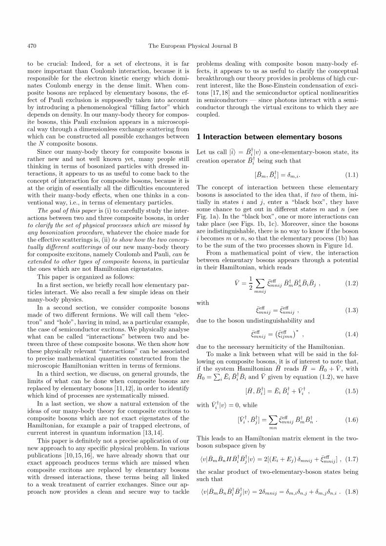
Fig. 1. (a) (resp. (e)): basic diagrams for the interactions oftwo (resp. three) elementary bosons. Between two compositebosons, one, two, or more interactions can exist as in (b) and(c), while two interactions at least are necessary (see (f)) tofind three composite bosons in “out” states (m, n, p) differentfrom the “in” states (i, j, k). Due to the boson undistinguisha-bility, the elementary scattering between two bosons must beinvariant under a (m ↔ n) and/or a (i ↔ j) permutation, asshown in (d).
If we now have three bosons entering the “black box”, twointeractions at least are necessary, in order to find thesebosons out of the box, all three in a state different from theinitial one (see Figs. 1e, 1f). Since ξeff
mnij has the dimensionof an energy, the second scattering of this two-interactionprocess has to appear along with an energy denominator.
2 Interactions between composite bosons
We now consider a composite boson made of two differentfermions. Let us call them “electron” and “hole”. The caseof composite bosons made of a pair of identical fermionswill be considered in the last part of this work. We labelthe possible states of this composite boson by i.
2.1 Two composite bosons
We start by considering two composite bosons in states iand j. From a conceptual point of view, an “interaction” is
a physical process which allows to bring these bosons intotwo different states, m and n. What can possibly happenin the “black box” of Figure 2a, to produce such a statechange?
2.1.1 Pure carrier exchange
The simplest process is, for sure, just a carrier exchange,either with the holes as in Figure 2b, or with the electronsas in Figure 2c. Since the two are physically similar, weexpect them to appear equally in a scattering λmnij basedon this pure exchange (see Fig. 2d). It is of interest tonote that the electron exchange of Figure 2c is equivalentto a hole exchange, with the (m, n) states permuted (seeFig. 2c’).
If this carrier exchange is repeated, we see from Fig-ure 2e that two hole exchanges reduce to an identity, i.e.,no scattering at all, while a hole exchange followed byan electron exchange results in a (m, n) permutation, i.e.,again no scattering at all for indistinguishable particles(see Fig. 2f).
Let us now show how we can make appearing the λmnij
exchange scattering formally. In view of Figure 2d, thisscattering has to read
2λmnij = λ(
nm
ji
)+ λ
(mn
ji
), (2.1)
where λ(
nm
ji
)corresponds to the hole exchange of Fig-
ure 2b, the excitons m and i having the same electron,
λ(
nm
ji
)=∫
dre drh dre′ drh′ 〈n|re′rh〉〈m|rerh′〉〈rerh|i〉〈re′rh′ |j〉 ,
(2.2)
where 〈rerh|i〉 is the wave function of the one-boson state|i〉. Note that the prefactor 2 of equation (2.1), whichcould be included in the definition of the Pauli scatter-ing, is physically linked to the fact that two exchanges arepossible in an electron-hole pair, namely a hole exchangeand an electron exchange. It is of interest to note that, inthe case of one electron and one exciton, as in problemsdealing with trions, these Pauli scatterings appear with-out any prefactor 2 because the exciton can only exchangeits electron with the electron gas.
If these one-boson states are orthogonal, 〈m|i〉 = δm,i,it is tempting to introduce the deviation-from-boson op-erator Dmi defined as
Dmi = δm,i − [Bm, B†i ], (2.3)
where B†i is the creation operator for the one-boson state
|i〉 = B†i |v〉. For δm,i = 〈m|i〉, this operator is such that
Dmi|v〉 = 0, (2.4)
472 The European Physical Journal B
(2a)
n
m
j
i
(2b)
rh’
rh
re
re’ j
i
n
m
m
n
j
i
n
m
j
i
(2c) (2c’)
=
= λnm
ji
n
m
j
i+
n
m
j
i 2 λmnij
(2d)
n
m
j
i
n
m
j
i=
(2e)
n
m
j
i
m
n
j
i=
(2f)
=
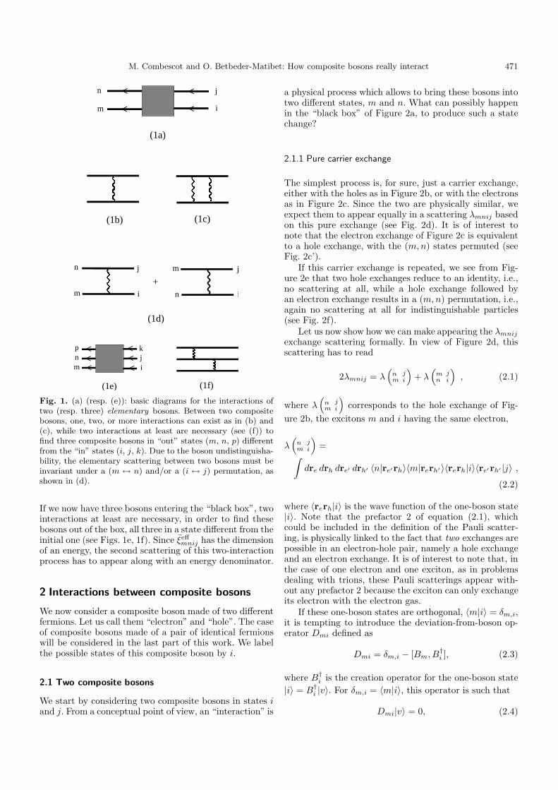
Fig. 2. (a) Basic diagram for the interaction of two compos-ite bosons made of an electron (solid line) and a hole (dashedline). (b) Elementary hole exchange λ
(n jm i
)between the “in”
composite bosons (i, j) and the “out” composite bosons (m,n). (c) Elementary electron exchange between the same com-posite bosons as the ones of (b). As shown in (c’), this electronexchange is equivalent to a hole exchange with (m, n) changedinto (n, m). (d) Due to the undistinguishability of the fermionsforming the composite bosons, the elementary Pauli scatteringλmnij between two composite bosons must be invariant undera (m ↔ n) and/or (i ↔ j) permutation. Due to (c, c′), thisPauli scattering must include a hole exchange and an electronexchange. (e) Two hole exchanges reduce to an identity. (f)One hole exchange followed by an electron exchange reducesto a (m, n) permutation: indeed, the resulting composite bo-son m is made with the same fermions as j. Note that all theseexchange processes are missed when composite bosons are re-placed by elementary bosons.
while its commutator with another boson creation opera-tor makes appearing the exchange or Pauli scatterings wewant, through
[Dmi, B†j ] = 2
∑n
λmnij B†n , (2.5)
as easy to see by calculating the scalar product of thetwo-boson states 〈v|BmBnB†
i B†j |v〉, using either the set of
commmutators (2.3, 5) or the two-composite-boson wavefunction,
〈re′rh′ , rerh|B†i B
†j |v〉 =
12
[〈rerh|i〉〈re′rh′ |j〉 − 〈re′rh|i〉〈rerh′ |j〉 + (i ↔ j)] .
(2.6)
This wave function is indeed invariant by (i ↔ j), as im-posed by B†
i B†j = B†
jB†i for B†’s being products of fermion
operators. It also changes sign under a (re, re′ ) exchange,as required by Pauli exclusion.
This leads to
〈v|BmBnB†i B
†j |v〉 = 2[δmnij − λmnij ]. (2.7)
This equation actually shows that the two-composite-boson states are nonorthogonal. This is just a bare conse-quence of the fact that these composite-boson states forman overcomplete basis [19]: Indeed, the composite-bosoncreation operators B†
i are such that
B†i B
†j = −
∑mn
λmnij B†mB†
n , (2.8)
easy to show by combining the fermion pairs in a differentway.
Due to B†i B
†j = B†
jB†i , equation (2.7) also shows that
λmnij = λmnji = λ∗ijmn . (2.9)
Finally, from the closure relation for one-boson states,∑i |i〉〈i| = I, it is easy to check that two exchanges reduce
to an identity, i.e.,∑rs
λmnrsλrsij = δmnij , (2.10)
with δmnij given in equation (1.8), as physically expectedfrom Figures 2e, 2f.
2.1.2 Direct and exchange Coulomb scatterings
If the two fermions are charged particles, another way forthese two composite bosons to interact is via Coulombinteraction between their carriers. The simplest of theseinteractions is a set of direct processes in which the outexcitons (m, n) are made with the same pair as the “in” ex-citons (i, j) (see Figs. 3a, 3b). However, here again, as thecarriers are indistinguishable, these processes must appear
M. Combescot and O. Betbeder-Matibet: How composite bosons really interact 473
rh’
re’
rh
re
n
m
j
iξ
nm
ji=
= + + +
(3a)
(3b)
n
m
j
i
m
n
j
i
+ = 2 ξmnij
(3c)
n
m
j
i
n
m
j
i
+ = 2 ξmnijin
(3d)
(3d’)
n
m
j
i
n
m
j
i
+ 2 ξmnijout=
(3e)
n
m
n
m
j
i
j
i
rh’
rh
re
re’
(3f) (3g)
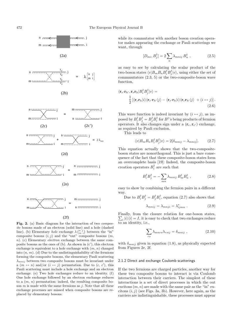
Fig. 3. (a) Elementary direct Coulomb scattering ξ(
n jm i
)be-
tween two composite bosons. (b) In this direct Coulomb scat-tering, enter the e–e, h–h as well as two e–h Coulomb inter-actions. (c) Due to the undistinguishability of the fermionsforming the composite bosons, the direct Coulomb scatteringξmnij between two composite bosons must be invariant un-der a (m ↔ n) and/or (i ↔ j) permutation, so that it iscomposed of two elementary direct Coulomb scatterings. (d)The “in” Coulomb scattering ξin
mnij corresponds to a directCoulomb scattering followed by a carrier exchange. As shownin (d’), the electron-hole Coulomb interaction of ξin
mnij is be-tween the “in” composite bosons, but inside the “out” ones. (e)The “out” Coulomb scattering ξout
mnij corresponds to a carrierexchange followed by a direct Coulomb interaction. (f) Pro-cesses in which the direct Coulomb interaction is followed bytwo hole exchanges reduce to a direct process. (g) Processesin which the hole exchanges are on both sides of the Coulombdirect interaction are physically strange because their electron-hole parts are “inside” both, the “in” and the “out” compositebosons, so that they are already counted in these compositebosons: We never find these strange processes appearing inphysical quantities resulting from many-body effects betweencomposite bosons.
in a scattering in which m and n are not differentiated, asin Figure 3c.
In view of Figures 3a, 3c, this direct Coulomb scatter-ing must read
2ξmnij = ξ(
nm
ji
)+ ξ
(mn
ji
), (2.11)
where, due to Figure 3a, ξ(
nm
ji
)is given by
ξ(
nm
ji
)=
∫dre drh dre′ drh′ 〈n|re′rh′〉〈m|rerh〉
× V (rerh; re′rh′) 〈rerh|i〉〈re′rh′ |j〉 ,
V (rerh; re′rh′) = Vee(re, re′) + Vhh(rh, rh′)+ Veh(re, rh′) + Veh(re′ , rh) . (2.12)
The potential V (rerh; re′rh′) is just the sum of theCoulomb interactions between an electron-hole pair madeof (e, h) and an electron-hole pair made of (e′, h′). Notethat, this Coulomb scattering being direct, the interactionsare between both, the “in” composite bosons (i, j) and the“out” composite bosons (m, n). From equations (2.11, 12),we see that this direct Coulomb scattering is such that
ξmnij = ξnmij = (ξijmn)∗ . (2.13)
Let us now make appearing this direct Coulomb scatter-ing ξmnij in a formal way. If the one-boson states |i〉 areeigenstates of the Hamiltonian, i.e., if
(H − Ei)B†i |v〉 = 0 , (2.14)
it is tempting to introduce the “creation potential” V †i
defined asV †
i = [H, B†i ] − EiB
†i . (2.15)
Due to equation (2.14), this operator is such that
V †i |v〉 = 0 . (2.16)
If, as for the Pauli scattering λmnij , we consider the com-mutator of this “creation potential” with another bosoncreation operator, we make appearing the direct Coulombscatterings we want, through
[V †i , B†
j ] =∑mn
ξmnij B†mB†
n . (2.17)
The derivation of this result, without taking an explicitform of the Hamiltonian, is however not as easy as the onefor λmnij , namely equation (2.5), because, due to the over-completeness of the composite-boson states which followsfrom equation (2.8), the ξmnij scattering of equation (2.17)can as well be replaced by (−ξin
mnij), where ξinmnij is an ex-
change Coulomb scattering defined as, (see Fig. 3d),
ξinmnij =
∑rs
λmnrs ξrsij . (2.18)
474 The European Physical Journal B
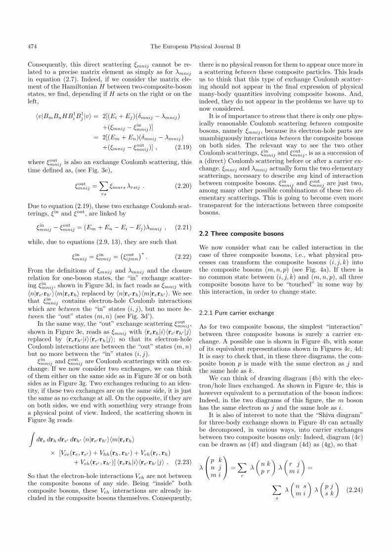
Consequently, this direct scattering ξmnij cannot be re-lated to a precise matrix element as simply as for λmnij
in equation (2.7). Indeed, if we consider the matrix ele-ment of the Hamiltonian H between two-composite-bosonstates, we find, depending if H acts on the right or on theleft,
〈v|BmBnHB†i B
†j |v〉 = 2[(Ei + Ej)(δmnij − λmnij)
+(ξmnij − ξinmnij)]
= 2[(Em + En)(δmnij − λmnij)
+(ξmnij − ξoutmnij)] , (2.19)
where ξoutmnij is also an exchange Coulomb scattering, this
time defined as, (see Fig. 3e),
ξoutmnij =
∑rs
ξmnrs λrsij . (2.20)
Due to equation (2.19), these two exchange Coulomb scat-terings, ξin and ξout, are linked by
ξinmnij − ξout
mnij = (Em + En − Ei − Ej)λmnij , (2.21)
while, due to equations (2.9, 13), they are such that
ξinmnij = ξin
nmij =(ξoutijmn
)∗. (2.22)
From the definitions of ξmnij and λmnij and the closurerelation for one-boson states, the “in” exchange scatter-ing ξin
mnij , shown in Figure 3d, in fact reads as ξmnij with〈n|re′rh′〉〈m|rerh〉 replaced by 〈n|re′rh〉〈m|rerh′〉. We seethat ξin
mnij contains electron-hole Coulomb interactionswhich are between the “in” states (i, j), but no more be-tween the “out” states (m, n) (see Fig. 3d’).
In the same way, the “out” exchange scattering ξoutmnij ,
shown in Figure 3e, reads as ξmnij with 〈rerh|i〉〈re′rh′ |j〉replaced by 〈rerh′ |i〉〈re′rh|j〉; so that its electron-holeCoulomb interactions are between the “out” states (m, n)but no more between the “in” states (i, j).
ξinmnij and ξout
mnij are Coulomb scatterings with one ex-change. If we now consider two exchanges, we can thinkof them either on the same side as in Figure 3f or on bothsides as in Figure 3g. Two exchanges reducing to an iden-tity, if these two exchanges are on the same side, it is justthe same as no exchange at all. On the opposite, if they areon both sides, we end with something very strange froma physical point of view. Indeed, the scattering shown inFigure 3g reads
∫dre drh dre′ drh′ 〈n|re′rh′〉〈m|rerh〉
× [Vee(re, re′ ) + Vhh(rh, rh′) + Veh(re, rh)+ Veh(re′ , rh′)] 〈rerh|i〉〈re′rh′ |j〉 . (2.23)
So that the electron-hole interactions Veh are not betweenthe composite bosons of any side. Being “inside” bothcomposite bosons, these Veh interactions are already in-cluded in the composite bosons themselves. Consequently,
there is no physical reason for them to appear once more ina scattering between these composite particles. This leadsus to think that this type of exchange Coulomb scatter-ing should not appear in the final expression of physicalmany-body quantities involving composite bosons. And,indeed, they do not appear in the problems we have up tonow considered.
It is of importance to stress that there is only one phys-ically reasonable Coulomb scattering between compositebosons, namely ξmnij , because its electron-hole parts areunambiguously interactions between the composite bosonson both sides. The relevant way to see the two otherCoulomb scatterings, ξin
mnij and ξoutmnij , is as a succession of
a (direct) Coulomb scattering before or after a carrier ex-change. ξmnij and λmnij actually form the two elementaryscatterings, necessary to describe any kind of interactionbetween composite bosons. ξin
mnij and ξoutmnij are just two,
among many other possible combinations of these two el-ementary scatterings. This is going to become even moretransparent for the interactions between three compositebosons.
2.2 Three composite bosons
We now consider what can be called interaction in thecase of three composite bosons, i.e., what physical pro-cesses can transform the composite bosons (i, j, k) intothe composite bosons (m, n, p) (see Fig. 4a). If there isno common state between (i, j, k) and (m, n, p), all threecomposite bosons have to be “touched” in some way bythis interaction, in order to change state.
2.2.1 Pure carrier exchange
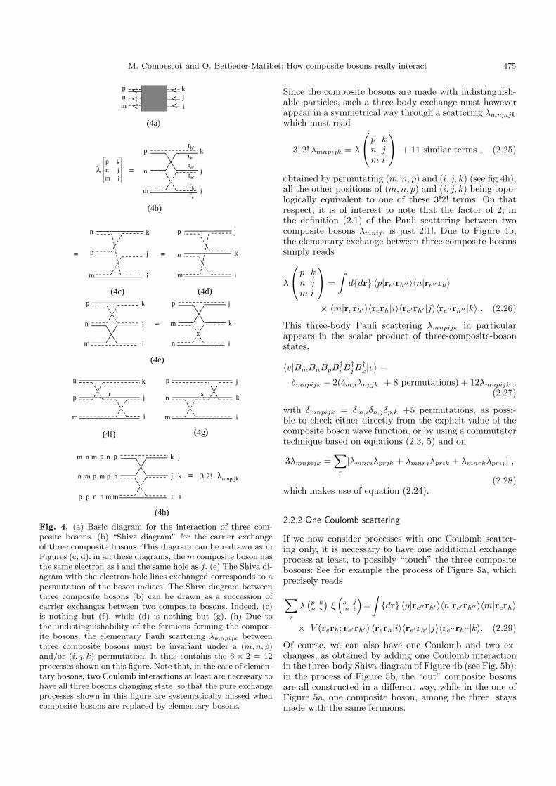
As for two composite bosons, the simplest “interaction”between three composite bosons is surely a carrier ex-change. A possible one is shown in Figure 4b, with someof its equivalent representations shown in Figures 4c, 4d:It is easy to check that, in these three diagrams, the com-posite boson p is made with the same electron as j andthe same hole as k.
We can think of drawing diagram (4b) with the elec-tron/hole lines exchanged. As shown in Figure 4e, this ishowever equivalent to a permutation of the boson indices:Indeed, in the two diagrams of this figure, the m bosonhas the same electron as j and the same hole as i.
It is also of interest to note that the “Shiva diagram”for three-body exchange shown in Figure 4b can actuallybe decomposed, in various ways, into carrier exchangesbetween two composite bosons only: Indeed, diagram (4c)can be drawn as (4f) and diagram (4d) as (4g), so that
λ
p k
n jm i
=
∑r
λ
(n kp r
)λ
(r jm i
)=
∑s
λ
(n sm i
)λ
(p js k
)(2.24)
M. Combescot and O. Betbeder-Matibet: How composite bosons really interact 475
pnm
kji
p
rh’
rh
re
re’
re’’
rh’’k
j
i
n
m
λpnm
kji
=
(4a)
(4b)
n
p
m
j
k
i
p
n
m
k
j
i
=
(4c) (4d)
=
j
k
i
m
n
k
j
i
n
m
p p
=
(4e)
k
j
i
k
i
n
p
m m
n
p
sr
(4f) (4g)
j
i
pn
m
n
m
pm
n
pm
p
n
m
n
p
m
n
p
k j
k
i
= 3!2! λmnpijk
(4h)
j
Fig. 4. (a) Basic diagram for the interaction of three com-posite bosons. (b) “Shiva diagram” for the carrier exchangeof three composite bosons. This diagram can be redrawn as inFigures (c, d): in all these diagrams, the m composite boson hasthe same electron as i and the same hole as j. (e) The Shiva di-agram with the electron-hole lines exchanged corresponds to apermutation of the boson indices. The Shiva diagram betweenthree composite bosons (b) can be drawn as a succession ofcarrier exchanges between two composite bosons. Indeed, (c)is nothing but (f), while (d) is nothing but (g). (h) Due tothe undistinguishability of the fermions forming the compos-ite bosons, the elementary Pauli scattering λmnpijk betweenthree composite bosons must be invariant under a (m,n, p)and/or (i, j, k) permutation. It thus contains the 6 × 2 = 12processes shown on this figure. Note that, in the case of elemen-tary bosons, two Coulomb interactions at least are necessary tohave all three bosons changing state, so that the pure exchangeprocesses shown in this figure are systematically missed whencomposite bosons are replaced by elementary bosons.
Since the composite bosons are made with indistinguish-able particles, such a three-body exchange must howeverappear in a symmetrical way through a scattering λmnpijk
which must read
3! 2! λmnpijk = λ
p k
n jm i
+ 11 similar terms , (2.25)
obtained by permutating (m, n, p) and (i, j, k) (see fig.4h),all the other positions of (m, n, p) and (i, j, k) being topo-logically equivalent to one of these 3!2! terms. On thatrespect, it is of interest to note that the factor of 2, inthe definition (2.1) of the Pauli scattering between twocomposite bosons λmnij , is just 2!1!. Due to Figure 4b,the elementary exchange between three composite bosonssimply reads
λ
p k
n jm i
=
∫d{dr} 〈p|re′rh′′〉〈n|re′′rh〉
× 〈m|rerh′〉〈rerh|i〉〈re′rh′ |j〉〈re′′rh′′ |k〉 . (2.26)
This three-body Pauli scattering λmnpijk in particularappears in the scalar product of three-composite-bosonstates,
〈v|BmBnBpB†i B
†jB
†k|v〉 =
δmnpijk − 2(δm,iλnpjk + 8 permutations) + 12λmnpijk ,(2.27)
with δmnpijk = δm,iδn,jδp,k +5 permutations, as possi-ble to check either directly from the explicit value of thecomposite boson wave function, or by using a commutatortechnique based on equations (2.3, 5) and on
3λmnpijk =∑
r
[λmnriλprjk + λmnrjλprik + λmnrkλprij ] ,
(2.28)which makes use of equation (2.24).
2.2.2 One Coulomb scattering
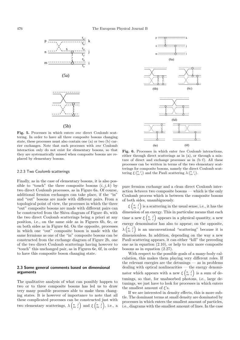
If we now consider processes with one Coulomb scatter-ing only, it is necessary to have one additional exchangeprocess at least, to possibly “touch” the three compositebosons: See for example the process of Figure 5a, whichprecisely reads
∑s
λ(pn
ks
)ξ(
sm
ji
)=
∫{dr} 〈p|re′′rh′〉〈n|re′rh′′〉〈m|rerh〉
× V (rerh; re′rh′) 〈rerh|i〉〈re′rh′ |j〉〈re′′rh′′ |k〉. (2.29)
Of course, we can also have one Coulomb and two ex-changes, as obtained by adding one Coulomb interactionin the three-body Shiva diagram of Figure 4b (see Fig. 5b):in the process of Figure 5b, the “out” composite bosonsare all constructed in a different way, while in the one ofFigure 5a, one composite boson, among the three, staysmade with the same fermions.
476 The European Physical Journal B
p
rh’
rh
re
re’’
rh’’k
j
i
n
m
re’
s
(5a)
(5b)
Fig. 5. Processes in which enters one direct Coulomb scat-tering. In order to have all three composite bosons changingstate, these processes must also contain one (a) or two (b) car-rier exchanges. Note that such processes with one Coulombinteraction only do not exist for elementary bosons, so thatthey are systematically missed when composite bosons are re-placed by elementary bosons.
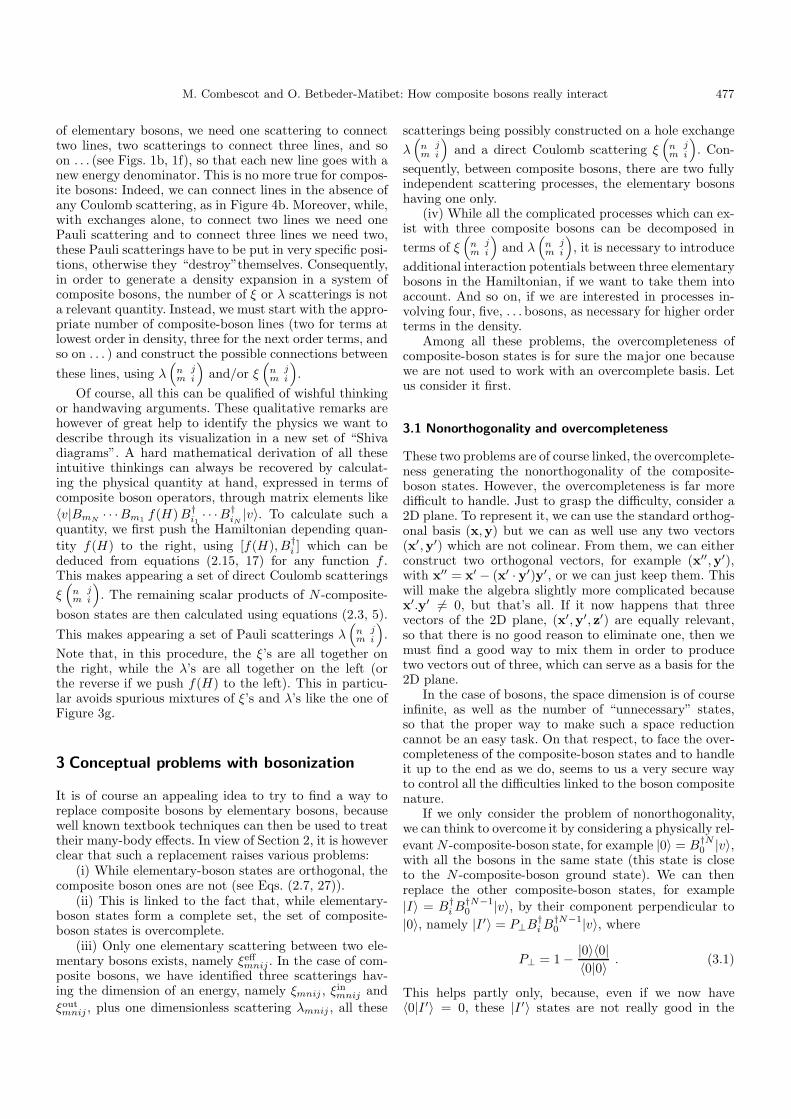
2.2.3 Two Coulomb scatterings
Finally, as in the case of elementary bosons, it is also pos-sible to “touch” the three composite bosons (i, j, k) bytwo direct Coulomb processes, as in Figure 6a. Of course,additional fermion exchanges can take place, if the “in”and “out” bosons are made with different pairs. From atopological point of view, the processes in which the three“out” composite bosons are made with different pairs canbe constructed from the Shiva diagram of Figure 4b, withthe two direct Coulomb scatterings being a priori at anyposition, i.e., on the same side as in Figures 6b, 6c, oron both sides as in Figure 6d. On the opposite, processesin which one “out” composite boson is made with thesame fermions as one of the “in” composite bosons can beconstructed from the exchange diagram of Figure 2b, oneof the two direct Coulomb scatterings having however to“touch” this unchanged pair, as in Figures 6e, 6f, in orderto have this composite boson changing state.
2.3 Some general comments based on dimensionalarguments
The qualitative analysis of what can possibly happen totwo or to three composite bosons has led us to drawvery many possible processes able to make them chang-ing states. It is however of importance to note that allthese complicated processes can be constructed just withtwo elementary scatterings, λ
(nm
ji
)and ξ
(nm
ji
), i.e., a
m
n
p k
j
i
(6a)
(6d)
(6b) (6c)
(6e) (6f)
Fig. 6. Processes in which enter two Coulomb interactions,either through direct scatterings as in (a), or through a mix-ture of direct and exchange processes as in (b–f). All theseprocesses can be written in terms of the two elementary scat-terings for composite bosons, namely the direct Coulomb scat-tering ξ
(n jm i
)and the Pauli scattering λ
(n jm i
).
pure fermion exchange and a clean direct Coulomb inter-action between two composite bosons — which is the onlyCoulomb process which is between the composite bosonsof both sides, unambiguously.
ξ(
nm
ji
)is a scattering in the usual sense, i.e., it has the
dimension of an energy. This in particular means that eachtime a new ξ
(nm
ji
)appears in a physical quantity, a new
energy denominator has also to appear; on the opposite,λ
(nm
ji
)is an unconventional “scattering” because it is
dimensionless. In addition, depending on the way a newPauli scattering appears, it can either “kill” the precedingone as in equation (2.10), or help to mix more compositebosons as in equation (2.27).
With respect to the possible goals of a many-body cal-culation, this makes them playing very different roles. Ifthe relevant energies are the detunings — as in problemsdealing with optical nonlinearities — the energy denomi-nator which appears with a new ξ
(nm
ji
)is a sum of de-
tunings, so that, for unabsorbed photons, i.e., large de-tunings, we just have to look for processes in which entersthe smallest amount of ξ’s.
If we are interested in density effects, this is more sub-tle. The dominant terms at small density are dominated byprocesses in which enters the smallest amount of particles,i.e., diagrams with the smallest amount of lines. In the case
M. Combescot and O. Betbeder-Matibet: How composite bosons really interact 477
of elementary bosons, we need one scattering to connecttwo lines, two scatterings to connect three lines, and soon . . . (see Figs. 1b, 1f), so that each new line goes with anew energy denominator. This is no more true for compos-ite bosons: Indeed, we can connect lines in the absence ofany Coulomb scattering, as in Figure 4b. Moreover, while,with exchanges alone, to connect two lines we need onePauli scattering and to connect three lines we need two,these Pauli scatterings have to be put in very specific posi-tions, otherwise they “destroy”themselves. Consequently,in order to generate a density expansion in a system ofcomposite bosons, the number of ξ or λ scatterings is nota relevant quantity. Instead, we must start with the appro-priate number of composite-boson lines (two for terms atlowest order in density, three for the next order terms, andso on . . . ) and construct the possible connections betweenthese lines, using λ
(nm
ji
)and/or ξ
(nm
ji
).
Of course, all this can be qualified of wishful thinkingor handwaving arguments. These qualitative remarks arehowever of great help to identify the physics we want todescribe through its visualization in a new set of “Shivadiagrams”. A hard mathematical derivation of all theseintuitive thinkings can always be recovered by calculat-ing the physical quantity at hand, expressed in terms ofcomposite boson operators, through matrix elements like〈v|BmN · · ·Bm1 f(H)B†
i1· · ·B†
iN|v〉. To calculate such a
quantity, we first push the Hamiltonian depending quan-tity f(H) to the right, using [f(H), B†
i ] which can bededuced from equations (2.15, 17) for any function f .This makes appearing a set of direct Coulomb scatteringsξ(
nm
ji
). The remaining scalar products of N -composite-
boson states are then calculated using equations (2.3, 5).This makes appearing a set of Pauli scatterings λ
(nm
ji
).
Note that, in this procedure, the ξ’s are all together onthe right, while the λ’s are all together on the left (orthe reverse if we push f(H) to the left). This in particu-lar avoids spurious mixtures of ξ’s and λ’s like the one ofFigure 3g.
3 Conceptual problems with bosonization
It is of course an appealing idea to try to find a way toreplace composite bosons by elementary bosons, becausewell known textbook techniques can then be used to treattheir many-body effects. In view of Section 2, it is howeverclear that such a replacement raises various problems:
(i) While elementary-boson states are orthogonal, thecomposite boson ones are not (see Eqs. (2.7, 27)).
(ii) This is linked to the fact that, while elementary-boson states form a complete set, the set of composite-boson states is overcomplete.
(iii) Only one elementary scattering between two ele-mentary bosons exists, namely ξeff
mnij . In the case of com-posite bosons, we have identified three scatterings hav-ing the dimension of an energy, namely ξmnij , ξin
mnij andξoutmnij , plus one dimensionless scattering λmnij , all these
scatterings being possibly constructed on a hole exchangeλ
(nm
ji
)and a direct Coulomb scattering ξ
(nm
ji
). Con-
sequently, between composite bosons, there are two fullyindependent scattering processes, the elementary bosonshaving one only.
(iv) While all the complicated processes which can ex-ist with three composite bosons can be decomposed interms of ξ
(nm
ji
)and λ
(nm
ji
), it is necessary to introduce
additional interaction potentials between three elementarybosons in the Hamiltonian, if we want to take them intoaccount. And so on, if we are interested in processes in-volving four, five, . . . bosons, as necessary for higher orderterms in the density.
Among all these problems, the overcompleteness ofcomposite-boson states is for sure the major one becausewe are not used to work with an overcomplete basis. Letus consider it first.
3.1 Nonorthogonality and overcompleteness
These two problems are of course linked, the overcomplete-ness generating the nonorthogonality of the composite-boson states. However, the overcompleteness is far moredifficult to handle. Just to grasp the difficulty, consider a2D plane. To represent it, we can use the standard orthog-onal basis (x,y) but we can as well use any two vectors(x′,y′) which are not colinear. From them, we can eitherconstruct two orthogonal vectors, for example (x′′,y′),with x′′ = x′ − (x′ · y′)y′, or we can just keep them. Thiswill make the algebra slightly more complicated becausex′.y′ �= 0, but that’s all. If it now happens that threevectors of the 2D plane, (x′,y′, z′) are equally relevant,so that there is no good reason to eliminate one, then wemust find a good way to mix them in order to producetwo vectors out of three, which can serve as a basis for the2D plane.
In the case of bosons, the space dimension is of courseinfinite, as well as the number of “unnecessary” states,so that the proper way to make such a space reductioncannot be an easy task. On that respect, to face the over-completeness of the composite-boson states and to handleit up to the end as we do, seems to us a very secure wayto control all the difficulties linked to the boson compositenature.
If we only consider the problem of nonorthogonality,we can think to overcome it by considering a physically rel-evant N -composite-boson state, for example |0〉 = B†N
0 |v〉,with all the bosons in the same state (this state is closeto the N -composite-boson ground state). We can thenreplace the other composite-boson states, for example|I〉 = B†
i B†N−10 |v〉, by their component perpendicular to
|0〉, namely |I ′〉 = P⊥B†i B
†N−10 |v〉, where
P⊥ = 1 − |0〉〈0|〈0|0〉 . (3.1)
This helps partly only, because, even if we now have〈0|I ′〉 = 0, these |I ′〉 states are not really good in the
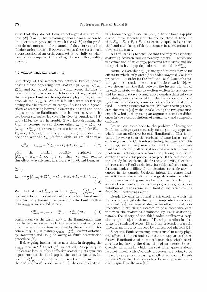
478 The European Physical Journal B
sense that they do not form an orthogonal set: we stillhave 〈J ′|I ′〉 �= 0. This remaining nonorthogonality can beunimportant in problems in which the 〈J ′|I ′〉 scalar prod-ucts do not appear — for example, if they correspond to“higher order terms”. However, even in these cases, sucha construction of an orthogonal set is not fully satisfac-tory, when compared to handling the nonorthogonality,properly.
3.2 “Good” effective scattering
Our study of the interactions between two compositebosons makes appearing four scatterings: ξmnij , ξin
mnij ,ξoutmnij and λmnij . Let us, for a while, accept the idea to
have bosonized particles which form an orthogonal set, sothat the pure Pauli scatterings do not play a role, i.e., wedrop all the λmnij ’s. We are left with three scatteringshaving the dimension of an energy. An idea for a “good”effective scattering between elementary bosons can be toimpose the same Hamiltonian matrix elements within thetwo-boson subspace. However, in view of equations (1.8)and (2.19), we are in trouble if we keep dropping theλmnij ’s, because we can choose either ξmnij − ξin
mnij orξmnij − ξout
mnij , these two quantities being equal for Em +En = Ei + Ej only, due to equation (2.21). If, instead, wedecide to keep the λmnij ’s for a while, we are led to take
ξeffmnij = ξmnij −
[ξinmnij + (Ei + Ej)λmnij
], (3.2)
with the bracket possibly replaced by[ξoutmnij + (Em + En)λmnij
]; so that we can rewrite
this effective scattering, in a more symmetrical form, as
ξeffmnij =
ξmnij − 12
[ξinmnij + ξout
mnij + (Em + En + Ei + Ej)λmnij
].
(3.3)
We note that this ξeffmnij is such that ξeff
mnij =(ξeffijmn
)∗, as
necessary for the hermiticity of the effective Hamiltonianfor elementary bosons. If we now drop the Pauli scatter-ings λmnij ’s, we are led to take
ξeffmnij = ξmnij − (ξin
mnij + ξoutmnij)/2 , (3.4)
which preserves the hermiticity of the Hamiltonian. Thishas to be contrasted with the effective scattering forbosonized excitons extensively used by the semiconductorcommunity [11,12], namely ξmnij−ξout
mnij , as first obtainedby Hanamura and Haug, following an Inui’s bosonizationprocedure [20].
Before going further, let us note that, in dropping theλmnij term in ξeff to get ξeff , we actually “drop” a quiteunpleasant feature of this effective scattering: its spuriousdependence on the band gap in the case of excitons. In-deed, in ξeff
mnij appears the sum — not the difference — ofthe “in” and “out” boson energies. In the case of excitons,
this boson energy is essentially equal to the band gap plusa small term depending on the exciton state at hand. Sothat Em + En + Ei + Ej is essentially equal to four timesthe band gap. Its possible appearance in a scattering is aphysical nonsense.
All this leads us to conclude that the only “reasonable”scattering between two elementary bosons — which hasthe dimension of an energy, preserves hermiticity and hasno spurious band gap dependence — should be ξeff
mnij .Actually, even this ξeff
mnij is not good, except may be foreffects in which only enter first order diagonal Coulombprocesses — in order for the “in” and “out” Coulomb scat-terings to be equal. Indeed, in a previous work [10], wehave shown that the link between the inverse lifetime ofan exciton state — due to exciton-exciton interations —and the sum of its scattering rates towards a different exci-ton state, misses a factor of 2, if the excitons are replacedby elementary bosons, whatever is the effective scatteringused — a quite strong statement! We have recently recov-ered this result [21] without calculating the two quantitiesexplicitly, but just by using an argument based on differ-ences in the closure relations of elementary and compositeexcitons.
Let us now come back to the problem of having thePauli scatterings systematically missing in any approachwhich uses an effective bosonic Hamiltonian. This is ac-tually far worse than the problem of choosing a “good”exchange part for Coulomb scattering, because, with thisdropping, we not only miss a factor of 2, but the domi-nant term [15,16] in all optical nonlinear effects! Indeed, aphoton interacts with a semiconductor through the virtualexciton to which this photon is coupled. If the semiconduc-tor already has excitons, the first way this virtual excitoninteracts is via Pauli exclusion, since this exclusion amongfermions makes it filling all the fermion states already oc-cupied in the sample. Coulomb interaction comes next,since it has to come with an energy denominator which,in problems involving unabsorbed photons, is a detuning,so that these Coulomb terms always give a negligible con-tribution at large detuning, in front of the terms comingfrom Pauli scatterings alone.
Beside the exciton optical Stark effect, in which theroots of our many-body theory for composite excitons canbe found [22], we have studied some other optical non-linearities in which the interaction of a composite exci-ton with the matter is dominated by Pauli scattering,namely the theory of the third order nonlinear suscep-tibility χ(3) [16], the theory of Faraday rotation in pho-toexcited semiconductors [23] and the precession of a spinpined on an impurity induced by unabsorbed photons [24].
Since this Pauli scattering, quite crucial in many phys-ical effects, is dimensionless, it cannot appear in the ef-fective Hamiltonian of bosonized particles, which needsa scattering having the dimension of an energy. Conse-quently, all terms in which this scattering appears alone,i.e., not mixed with Coulomb processes, are going to bemissed by any procedure using an effective bosonic Hamil-tonian. (Note that this is also true for any approach usinga spin-spin Hamiltonian [13]).
M. Combescot and O. Betbeder-Matibet: How composite bosons really interact 479
Finally, our qualitative discussion on the possible in-teractions between three composite bosons, has led us toidentify, in addition to pure exchange processes based onPauli scattering between three composite bosons, againmissed, more complicated mixtures of Coulomb and ex-change than the one appearing between two compositebosons, ξin
mnij and ξoutmnij . In order not to miss them, we
could think of adding a three-body part to the Hamilto-nian like
V ′ =13!
∑mnpijk
ξeffmnpijk B†
mB†nB†
pBiBjBk . (3.5)
Let us however note that the proper identification ofξeffmnpijk with the three-body processes not constructed
from ξmnij , ξinmnij and ξout
mnij , is quite tricky, because thisthree-body potential formally contains terms in which oneelementary boson can stay unchanged, i.e., terms alreadyincluded in V .
All this actually means that the “good” effectivebosonic Hamiltonian, apart from the pure Pauli termswhich are going to be missed anyway, has to be more andmore complicated if we want to include processes in whichmore and more bosons are involved, i.e., if we want tostudy many-body effects, really. Just for that, the replace-ment of composite bosons by elementary boson seems tous far more complicated than keeping the boson compositenature through a set of Pauli scatterings, as we propose.
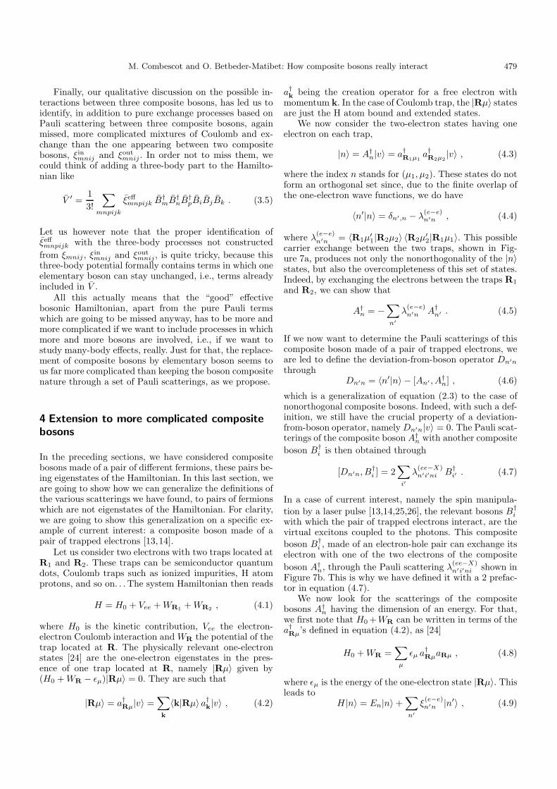
4 Extension to more complicated compositebosons
In the preceding sections, we have considered compositebosons made of a pair of different fermions, these pairs be-ing eigenstates of the Hamiltonian. In this last section, weare going to show how we can generalize the definitions ofthe various scatterings we have found, to pairs of fermionswhich are not eigenstates of the Hamiltonian. For clarity,we are going to show this generalization on a specific ex-ample of current interest: a composite boson made of apair of trapped electrons [13,14].
Let us consider two electrons with two traps located atR1 and R2. These traps can be semiconductor quantumdots, Coulomb traps such as ionized impurities, H atomprotons, and so on. . . The system Hamiltonian then reads
H = H0 + Vee + WR1 + WR2 , (4.1)
where H0 is the kinetic contribution, Vee the electron-electron Coulomb interaction and WR the potential of thetrap located at R. The physically relevant one-electronstates [24] are the one-electron eigenstates in the pres-ence of one trap located at R, namely |Rµ〉 given by(H0 + WR − εµ)|Rµ〉 = 0. They are such that
|Rµ〉 = a†Rµ|v〉 =
∑k
〈k|Rµ〉 a†k|v〉 , (4.2)
a†k being the creation operator for a free electron with
momentum k. In the case of Coulomb trap, the |Rµ〉 statesare just the H atom bound and extended states.
We now consider the two-electron states having oneelectron on each trap,
|n〉 = A†n|v〉 = a†
R1µ1a†R2µ2
|v〉 , (4.3)
where the index n stands for (µ1, µ2). These states do notform an orthogonal set since, due to the finite overlap ofthe one-electron wave functions, we do have
〈n′|n〉 = δn′,n − λ(e−e)n′n , (4.4)
where λ(e−e)n′n = 〈R1µ
′1|R2µ2〉 〈R2µ
′2|R1µ1〉. This possible
carrier exchange between the two traps, shown in Fig-ure 7a, produces not only the nonorthogonality of the |n〉states, but also the overcompleteness of this set of states.Indeed, by exchanging the electrons between the traps R1
and R2, we can show that
A†n = −
∑n′
λ(e−e)n′n A†
n′ . (4.5)
If we now want to determine the Pauli scatterings of thiscomposite boson made of a pair of trapped electrons, weare led to define the deviation-from-boson operator Dn′nthrough
Dn′n = 〈n′|n〉 − [An′ , A†n] , (4.6)
which is a generalization of equation (2.3) to the case ofnonorthogonal composite bosons. Indeed, with such a def-inition, we still have the crucial property of a deviation-from-boson operator, namely Dn′n|v〉 = 0. The Pauli scat-terings of the composite boson A†
n with another compositeboson B†
i is then obtained through
[Dn′n, B†i ] = 2
∑i′
λ(ee−X)n′i′ni B†
i′ . (4.7)
In a case of current interest, namely the spin manipula-tion by a laser pulse [13,14,25,26], the relevant bosons B†
iwith which the pair of trapped electrons interact, are thevirtual excitons coupled to the photons. This compositeboson B†
i , made of an electron-hole pair can exchange itselectron with one of the two electrons of the compositeboson A†
n, through the Pauli scattering λ(ee−X)n′i′ni shown in
Figure 7b. This is why we have defined it with a 2 prefac-tor in equation (4.7).
We now look for the scatterings of the compositebosons A†
n having the dimension of an energy. For that,we first note that H0 +WR can be written in terms of thea†Rµ’s defined in equation (4.2), as [24]
H0 + WR =∑
µ
εµ a†RµaRµ , (4.8)
where εµ is the energy of the one-electron state |Rµ〉. Thisleads to
H |n〉 = En|n〉 +∑n′
ξ(e−e)n′n |n′〉 , (4.9)

480 The European Physical Journal B
R2 µ2
R1 µ1
R2 µ’2
R1 µ’1
n’ n = λn’n(e-e)
R2R2
R1R1
nn’
ii’
nn’
ii’
+ 2 λn’i’ni(ee-X)=
R2R1
R2R1
R2R1
nn’
ii’ii’ii’
nn’nn’
= + = ξn’i’ni(ee-X)
R2 µ2
R1 µ1
R2 µ’2
R1 µ’1
=nn’ ξn’n(e-e)
(7a)
(7b)
(7c)
(7d)
Fig. 7. (a) Pauli scattering λ(e−e)n′n between two electrons
trapped in R1 and R2. In this exchange, the electrons canend in trapped states n′ = (µ′
1, µ′2) different from the initial
ones n = (µ1, µ2). (b) Pauli scattering λ(ee−X)n′i′ni between a com-
posite boson made of a trapped electron pair and a compositeboson made of an electron-hole pair, i.e., more precisely a com-posite exciton, their states changing from (n, i) to (n′, i′). (c)
Direct scattering ξ(e−e)n′n between two trapped electrons. This
scattering contains the Coulomb interaction between the twoelectrons as well as the interactions of each electron with thepotential of the other trap. (d) Direct scattering ξ
(ee−X)
n′i′ni be-tween a composite boson made of a trapped electron pair anda composite exciton. This scattering contains the Coulomb in-teraction of the exciton with each of the two trapped electrons.
where En = εµ1 + εµ2 is the “free” energy of the pair oftrapped electrons, while ξ
(e−e)n′n , shown in Figure 7c, comes
from their Coulomb repulsion as well as from the interac-tion of each electron with the other trap.
For such composite bosons A†n, which, due to equa-
tion (4.9), are not eigenstates of the Hamiltonian, theproper way to define their “creation potential” is through
V †n = [H, A†
n] − EnA†n −
∑n′
ξ(e−e)n′n A†
n′ , (4.10)
in order to still have V †n |v〉 = 0, equation (4.10) being a
generalization of equation (2.15). We then get the “directCoulomb scattering” between the composite boson A†
n andanother composite boson B†
i , through
[V †n , B†
i ] =∑n′i′
ξ(ee−X)n′i′ni A†
n′B†i′ , (4.11)
which is similar to equation (2.17). This direct scatter-ing is shown in Figure 7d. It corresponds to the directCoulomb interaction of each of the two trapped electronswith the electron-hole pair of the exciton.
Using this set of commutators and the two scatteringsλ
(e−e)n′n and ξ
(e−e)n′n they generate, we are going to calcu-
late the energy of two trapped electrons with their possi-ble exchanges included exactly, in order to determine thesinglet-triplet splitting these exchange processes induce inthe van der Waals energy. Using them and the two scat-terings between the trapped pair and an exciton, λ
(ee−X)n′n
and ξ(ee−X)n′n , we are also going to calculate the splitting of
the trapped electron pair energy induced by virtual exci-tons coupled to a laser beam, which results from electronexchanges between the trapped pair and the electron ofthe virtual exciton. This last problem is of great currentinterest for the control of the spin transfer time betweentwo traps using a laser pulse, with, in mind, its possibleuse for quantum information [27].
5 Conclusion
In this paper, we have made a detailed qualitative analysisof what can be called “interaction” between two or threecomposite bosons. We have shown that all the processeswhich produce a change in the boson states, can be writtenin terms of two scatterings only: a direct Coulomb scatter-ing which has the dimension of an energy and a pure Pauli“scattering” which is dimensionless. This Pauli scatteringis actually the novel ingredient of our many-body theoryfor composite bosons in which these composite bosons arenever replaced by elementary bosons.
We can possibly think of including processes in whichenter complicated mixtures of direct Coulomb scatteringsand Pauli scatterings, through a set of effective scatteringsbetween two, three, or more elementary bosons. On the op-posite, all processes in which the Pauli scatterings appearalone have to be missed if one uses effective Hamiltoni-ans such as the ones in which the composite bosons arereplaced by elementary bosons, or any spin-spin Hamil-tonian, whatever the effective coupling is. This, in par-ticular, happens in all semiconductor optical nonlineari-ties, the virtual exciton coupled to the photon field feelingthe presence of the fermions present in the sample, “evenmore” than their charges.
Finally, we have shown how to extend the mathe-matical definitions of the Pauli scattering and the di-rect Coulomb scattering to non trivial composite bosonswhich are not eigenstates of the Hamiltonian, such asa pair of trapped electrons. This extension again goesthrough the introduction of “deviation-from-boson oper-ators” and “creation potentials”, the main characteristicof these quantities being to give zero when they act onvacuum, so that they really describe interactions with therest of the system.
Although it is easy to understand the reluctance onemay have to enter a new way of thinking interactions be-tween composite bosons, it appears to us as worthwhileto spend the necessary amount of time to grasp these newideas, in view of their potentiality in very many problemsof physics.
M. Combescot and O. Betbeder-Matibet: How composite bosons really interact 481
References
1. A.A. Abrikosov, L.P. Gorkov, I.E. Dzyaloshinski, Methodsof quantum field theory in statistical physics (Prentice-Hall, Englewood Cliffs, N.J., 1964)
2. P. Nozieres, Le probleme a N Corps (Dunod, Paris, 1963)3. A. Fetter, J. Walecka, Quantum theory of many-particle
systems (Mc Graw-Hill, N.Y., 1971)4. G. Mahan, Many-particle physics (Plenum Press, N.Y.,
1990)5. For a review, see A. Klein, E.R. Marshalek, Rev. Mod.
Phys. 63, 375 (1991), and references therein6. For a short review, see M. Combescot, O. Betbeder-
Matibet, Solid State Com. 134, 11 (2005)7. M. Combescot, O. Betbeder-Matibet, Europhysics Lett.
58, 87 (2002); M. Combescot, O. Betbeder-Matibet,Europhysics Lett. 62, 140 (2003)
8. O. Betbeder-Matibet, M. Combescot, Eur. Phys. J. B 27,505 (2002)
9. M. Combescot, O. Betbeder-Matibet, Eur. Phys. J. B 42,509 (2004)
10. M. Combescot, O. Betbeder-Matibet, Phys. Rev. Lett. 93,016403 (2004)
11. E. Hanamura, H. Haug, Phys. Rep. 33, 209 (1977)12. H. Haug, S. Schmitt-Rink, Prog. Quant. Elect. 9, 3 (1984)13. C. Piermarocchi, C. Chen, L.J. Sham, D.J. Steel, Phys.
Rev. Lett. 89, 167402-1 (2002)
14. A. Nazir, B. Lovet, S.D. Barrett, T.P. Spiller, G.A.D.Briggs, Phys. Rev. Lett. 93, 150502-1 (2004)
15. M. Combescot, R. Combescot, Phys. Rev. Lett. 61, 117(1988)
16. M. Combescot, O. Betbeder-Matibet, K. Cho, H. Ajiki,Europhys. Lett. 72, 618 (2005)
17. D. Snoke, Science 298, 1368 (2002)18. L.V. Butov, A.C. Gossard, D.S. Chemla, Nature 418, 751
(2002)19. As pointed out long ago by M. Girardeau, J. Math. Phys.
4, 1096 (1963)20. T. Usui, Prog. Theor. Phys. 23, 787 (1957)21. M. Combescot, O. Betbeder-Matibet, Phys. Rev. B 72,
193105 (2005)22. For a review, see M. Combescot, Phys. Rep. 221, 168
(1992)23. M. Combescot, O. Betbeder-Matibet, submitted to Phys.
Rev. B24. M. Combescot, O. Betbeder-Matibet, Solid State Com.
132, 129 (2004)25. A. Imamoglu et al., Phys. Rev. Lett. 83, 4204 (1999)26. M.N. Leuenberger, M.E. Flatte, D.D. Awschalom, Phys.
Rev. Lett. 94, 107401 (2005)27. See for example, Semiconductor spintonics and quantum
computation, edited by D.D. Awschalom, D. Loss, N.Samarth (Springer, N.Y., 2002)