how committed are bank lines of credit? experiences in the ... · ratings, commitment status, etc.)...
TRANSCRIPT

WORKING PAPER NO. 10-25 HOW COMMITTED ARE BANK LINES OF CREDIT?
EXPERIENCES IN THE SUBPRIME MORTGAGE CRISIS
Rocco Huang
Federal Reserve Bank of Philadelphia
August 10, 2010

How Committed Are Bank Lines of Credit? Experiences in the Subprime Mortgage Crisis
Rocco Huang*
Federal Reserve Bank of Philadelphia
August 10, 2010
Abstract
Using the subprime mortgage crisis as a shock, this paper shows that commercial borrowers served by more distressed banks (as measured by recent bank stock returns or the nonperforming loan ratio) took down fewer funds from precommitted, formal lines of credit. The credit constraints affected mainly smaller, riskier (by internal loan ratings), and shorter-relationship borrowers, and depended also on the lenders’ size, liquidity condition, capitalization position, and core deposit funding. The evidence suggests that credit lines provided only contingent and partial insurance during the crisis since bank conditions appeared to influence credit line utilization in the short term. It provides a new explanation as to why credit lines are not perfect substitutes for cash holdings for some (e.g. small) firms. Finally, loan level analyses show that more distressed banks charged higher credit spreads on newly negotiated loans but not on funds disbursed from precommitted, formal credit lines. Our analyses are based on commercial loan flow data from the confidential Survey of Terms of Business Lending (STBL).
* I would like to thank Viral Acharya, Allen Berger, Mitch Berlin, Christa Bouwman, Stijn Claessens, Michael Faulkender, Paolo Fulghieri, Paul Gao, Mariassunta Giannetti, Itay Goldstein, Victoria Ivashina, Luc Laeven, Mamid Mehran, Don Morgan, Leonard Nakamura, Amir Sufi, Anjan Thakor, Greg Udell, and the audience at the FDIC Annual Banking Conference, NYU Stern/New York Fed Annual Conference on Financial Intermediation, for their helpful comments and suggestions. The views expressed here are those of the author and do not necessarily represent the views of the Federal Reserve Bank of Philadelphia or the Federal Reserve System. This paper is available free of charge at www.philadelphiafed.org/research-and-data/publications/working-papers/.

1
Below a CFO explained why her company drew down $2 billion from its credit line in
September and October 2008, “to enhance [its] cash position.”
David M. Katz (CFO Magazine, Dec 16, 2008): Are you using the cash you’ve drawn
from those credit lines? What’s the virtue in drawing down lines of credit and paying interest
on debt you are using?
Holly Koeppel (CFO of AEP, one of the nation’s biggest generators of electricity):
That’s that negative carry. It’s nice to have money in the bank …
Katz: But these were existing lines that you could have drawn down at any time. Was
there some underlying worry about whether banks could deliver when you needed it?
Koeppel: At the time of the first draw, no. After Lehman, I was not worried about our
principal banking relationships, but I certainly felt more comfortable knowing that I had the
money in the bank and we were very, very liquid. We’ve had very strong support from our
bank group. We’re very grateful for their relationship and support. But I sleep better knowing
that we have enough money in the bank.
I. Introduction
Why does a CFO need to worry about her company’s access to a legally binding
bank line of credit? Maybe bank lines of credit are not as committed as they seem, and
maybe there are times when a borrower needs to worry about a lender’s credit rating.
Koeppel was not alone. Mark Shamber (CFO of United Natural Foods, which has a $400
million credit facility with banks) reportedly “now carefully tracks the financial reports of
the publicly traded members of his bank group.”
A formal credit line (sometimes known as a revolving credit facility or a loan
commitment) is a legally binding commitment for which a bank has charged a fee, which
allows the borrower to take down funds at a certain spread over a base rate. Bank lines of
credit and cash holdings are the two most popular liquidity management tools used by
corporations (Lins, Servaes, and Tufano, 2007). Sufi (2007) finds that 85% of firms in his
sample obtained a line of credit between 1996 and 2003, and the line of credit represents
an average of 16% of book assets. In Lins et al.’s (2007) international sample, the median
line of credit is equal to 15% of book assets, whereas cash holdings comprise only 9%
(among which only 40% are not tied up for day-to-day operations).
The theoretic literature considers lines of credit as committed liquidity insurance
(Boot, Thakor, and Udell, 1987; Berkovitch and Greenbaum, 1991; Duan and Yoon,
2
1993; Holmstrom and Tirole, 1998; Morgan, 1994; Shockley, 1995; and Thakor, 2005).
The literature also shows that depository banks have a natural advantage in providing
liquidity under lines of credits (Kashyap, Stein, and Rajan, 2002; Gatev and Strahan,
2006, 2008; Nini, 2008; Gatev, Schuermann, and Strahan, 2009).
However, the empirical literature on corporate cash holdings finds that firms, and
in particular smaller firms, rely a lot on cash for liquidity management (Almeida,
Campello, and Weisbach, 2004; Faulkender and Wang 2006; Opler et al. 1999; Duchin,
Ozbas, Sensoy, 2008), suggesting that lines of credit do not provide sufficient liquidity
insurance for all firms. Sufi (2007) finds that banks provide credit lines that are
contingent on maintenance of cash flow and that lines of credit are therefore a poor
liquidity substitute for firms that have low existing or expected cash flows.
In this paper we provide an additional explanation as to why bank lines of credit
are contingent but not committed sources of liquidity insurance for certain types of firms.
Specifically, we show that provision of credit in committed lines of credit is sensitive
also to the banks’ own financial conditions.
At first sight, precommitted credit lines provide committed insurance for
borrowers because both credit limits and terms are set ex-ante and they are legally
binding promises. However, we believe that banks can exploit at least two sources of
bargaining power to influence credit line takedown volumes.
The first source of power comes from financial covenants. Credit line facilities
typically come with financial covenants (Bradley and Roberts, 2003; Chava and Roberts
2007) to mitigate agency problems (Aghion and Bolton, 1992; Berlin and Mester, 1992;
Dewatripont and Tirole, 1994). When a firm breaches a financial covenant, it triggers a
“technical default.” Chava and Roberts (2007) find that about 15% of borrowers are in
violation at any point in time and more than a third of borrowers are in violation at some
point during their ten-year sample period. However, creditors typically renegotiate the
contract, and covenant breaches rarely lead to default or acceleration of the loan
(Gopalakrishnan and Parkash, 1995). Arguably, financial covenant violations may
become even more common during an economic downturn when many borrowers’ sales
and cash flows are negatively affected (but they are not necessarily distressed).

3
The second source of power comes from a “borrowing base” requirement. More
than 80% of precommitted credit lines in our sample are secured, but not by real estate
collateral. They are most likely credit facilities with a “borrowing base,” which is a
lending formula that limits borrowings to a certain percentage of collateral, the most
common being receivables and inventory. Banks reserve the right to regularly check the
collateral, but they also have discretion over the frequency and rigor of auditing.
Anecdotal reports in the media (CFO Magazine, May 19, 2009) suggest that, during the
crisis, in particular when banks experienced their own capital and liquidity problems and
were pressured by regulators, audits of borrowers’ working capital became more
frequent, which often led to the reduction of loan capacity because many borrowers were
sitting on inventories that had depreciated greatly in value.
Therefore, we hypothesize that a bank retains significant influence over credit
line utilization because it has discretion over whether to waive the borrowers’ current or
future compliance with financial covenants or the borrowing base requirement, and
therefore credit lines provide only partial and contingent insurance for borrowers. A bank
may not invoke the discretion when it is in good financial health. When needed, however,
a bank can directly influence credit line takedown volumes by reducing credit availability
to borrowers who are not in compliance with covenants or whose collateral (inventory
and receivables) has declined in value. A threat of doing so (e.g., auditing collateral) can
also persuade less urgent borrowers from withdrawing funds when the bank is in distress.
We use the subprime mortgage crisis (prior to the direct injection of TARP money
into bank equity) as a shock to conduct our tests, during which banks experienced severe
deteriorations in financial health but the level of distress varied a lot across lenders and
over time. We then study how the financial distress that originated in the residential real
estate sector affected the new supply of loans to commercial and industrial borrowers
(excluding any real estate loans).
Our analyses are based on the confidential Survey of Terms of Business Lending
(STBL) data collected by the Federal Reserve, which contain rich information (loan risk
ratings, commitment status, etc.) on new commercial loans made by surveyed banks
during the first business week of every February, May, August, and November. The data
allow us to measure new loan flows, which most other data sets do not.

4
During the crisis, banks in distress, in order to preserve their own liquidity and
capital, if they have the discretion, may have incentives not to honor all liquidity demand
from borrowers (Boot, Greenbaum and Thakor, 1993). In a panel of 120 banks over 7
quarters, we empirically show that in more distressed banks (as measured by recent stock
returns or the nonperforming loan ratio), pre-committed credit lines reported smaller
takedown volumes. Further, we find that the impacts were concentrated on risky
borrowers, smaller borrowers, and borrowers with shorter relationships with the banks.
We also find that smaller, less liquid, less capitalized, and less retail-deposit-funded
banks responded more strongly to their own conditions. The results on the importance of
deposit funding are consistent with Ivashina and Scharfstein (2008). However, we also
study smaller loans not available in the Dealscan database used in their study.
Distinguishing between large and small borrowers provides important, new insights.
Analyzing loan-level data, we also find that in response to the deterioration in
their own financial health, banks raised interest rates on new term loans, loans from
informal credit lines, and new formal credit lines, but not in precommitted formal credit
lines, in which we observe declines in quantities instead.
We are not the first to show that the loan volume from precommitted credit lines
is surprisingly influenced also by supply-side factors. Berger and Udell’s (1992) study
focuses on two “credit crunch” episodes (1978:2-1980:1, 1981:1-1981:4) and they also
show that when credit markets are tight, loans disbursed from committed lines are
rationed when the commitments should have contractually protected borrowers from
rationing. Loan commitments may not be as committed as they seem.
The evidence is inconsistent with the notion that formal credit lines provided
committed insurance for borrowers, because takedown volumes in truly committed
facilities should be affected only by borrowers’ conditions (such as cash flow as
documented by Campello, Giambona, Graham, and Harvey, 2009) and not the lenders’
conditions. The results provide a new explanation as to why bank credit lines are not
perfect substitutes for cash, because access to credit lines is contingent on bank
performance in addition to the borrower’s own creditworthiness.
Our data and analyses have several key limitations. We do not have information
on the identity of the borrowers and therefore are unable to control for industry and

5
accounting performance of the borrowers. We can only make inference about the size of
the borrowers through the size of the credit line facility and about the riskiness of the
borrowers through internal risk ratings of loans. Finally, while databases like Dealscan
observe facilities’ initiations but not takedowns, we in contrast observe takedowns but do
not have information on credit facilities that were not drawn upon during the survey
weeks. To sum up, we do not know whether borrower demand may have driven the
results. Similar to Kashyap and Stein (2000), we draw our conclusion based on the
assumption that loan demand does not systematically correlate with variations in lender
financial conditions, in particular when those variations originate from exposures in the
residential mortgage sector, which are not directly related to the loan demand of
commercial borrowers.
Our paper is related to several literatures. First, the literature on how bank
performance affects credit supply, including Kang and Stulz (2000), Ongena, Smith, and
Michalsen (2003), Khwaja and Mian (2008), Paravisini (2007), and Berger and
Bouwman (2008, 2009), Schnabl (2009), Puri, Rocholl, and Steffen (2009). More
broadly, the literature on how stock market returns affect real investment, including
Blanchard, Rhee, and Summers (1993), Baker, Stein, Wurgler (2003), Chen, Goldstein,
and Jiang (2006).
Second, the literature on why credit lines are not perfect substitutes for cash,
including Sufi (2007). Ivashina and Scharfstein (2008), for example, find that many firms
drew down their credit lines and kept the proceeds in low-yielding cash, leading to a
“negative carry.”1 The borrowers’ actions can be explained if they worry about their
banks’ potential future distress, in light of our findings that credit lines from distressed
banks are not as reliable a source of liquidity. Campello et al. (2009), using survey data,
find that more credit-constrained firms are more likely to preemptively draw on their
lines of credits. Their actions are again understandable because those types of borrowers
are most likely to be rationed when their lenders are having their own problems.
Finally, our results are important because research has shown that access to bank
credit affects corporate financing and real investment policies (Roberts and Sufi, 2008a;
1 A typical explanation in a company’s 10-Q goes like this: “the Company had no immediate needs for additional liquidity; in light of the then current financial market conditions, the Company drew on the facility to provide it with greater financial flexibility.”
6
Lemmon and Roberts, 2007; Chava and Roberts, 2007; Chava and Purnanandam, 2008;
Almeida, Campello, and Hackbarth, 2009; Almeida, Campello, Laranjeira, and
Weisbenner, 2009; Gao and Yun, 2009).
The rest of the paper is organized as follows. In Section II, we use the Survey of
Terms of Business Lending to describe the commercial loan market in the US. In Section
III, we present our main regression specifications and analyze takedown volumes of
formal credit lines by borrower type and bank type. We also analyze loan pricing using
individual loan-level data. In Section IV we conclude.
II. Empirical Design
A. Survey of Terms of Business Lending
Our primary data source is the confidential Survey of Terms of Business Lending
(STBL) conducted by the Federal Reserve. The micro-data have been used in many other
papers, including Berger and Udell (1992, 2004), Lang and Nakamura (1995), Berger,
Saunders, Scalise, and Udell (1998), Berlin and Mester (1999), Berger, Espinoza-Vega,
Frame, and Miller (2005), Erel (2007) and Vickery (2008). The Federal Reserve’s
statistical release E.2., made public with a one-month lag, provides aggregate numbers
from the STBL. The micro-data remain confidential information.
The surveys take a snapshot of one week of new loan flows every 13 weeks. If the
survey weeks are representative, our data should include about 7.7% of all new loan
flows from a bank. The data cover all commercial and industrial (C&I) loans (new loans,
takedowns under revolving credit agreements, and renewals) made by a surveyed bank to
US addresses with a face value of at least $3,000, disbursed by surveyed banks during the
first business week of every February, May, August, and November.
These loans are arguably not directly affected by the problems in the subprime
mortgage sector, because the surveys exclude construction and land development loans
secured by real estate and loans to financial institutions. Existing loans on which the rates
are repriced when no additional funds are disbursed are also excluded. The surveys cover
both large syndicated loans studied extensively by many previous papers (typically based
on the Dealscan database) and smaller and bilateral loans. The largest loan made during
7
our sample period was about $600 million and the largest commitment was about $60
billion.2
One of the strengths of the data set is that it covers the new flow of loans. Publicly
available data typically report end-of-period outstanding loan volumes and unused
commitments. However, both an increase in takedowns and the termination of existing
lines can reduce unused commitment numbers, and outstanding loan volume numbers can
be affected by new loans, takedowns from existing revolvers, or retirement of existing
loans. With end-of-period measures, it is impossible to pin down the timing and causes of
the end-of-period changes. The STBL data also include rich information on loan
characteristics such as a loan’s risk rating and commitment status (formal or informal).
One of the weaknesses is that we do not know much about the borrowers, except
some proxies for borrower size, risk, and bank-firm relationship length. Most important,
although we know the amount of undrawn credits one month prior to the drawdown, we
do not have information on individual credit lines that were not drawn upon during the
survey weeks. In our econometric analyses, this shortcoming necessitates aggregating
individual loan disbursements to the bank level and estimating models with bank fixed
effects, assuming that the composition of existing credit lines does not change much
within a short period of time for a bank.
We focus on banks belonging to publicly traded bank holding companies, because
their stock returns provide a real-time summary measure of individual bank performance,
and such returns are more difficult to manipulate than accounting numbers. Since it is
relatively easy to issue public equities in the US, only very small banks are excluded
because of this restriction. The smallest publicly traded bank in our sample manages only
about $120 million in total assets.
In order to estimate a fixed-effect panel regression model, we require that banks
in our sample must have participated in the STBL at least twice. The survey collects data
from about 250 domestic commercial banks each time, and our final sample includes
2 For confidentiality reasons, the two numbers reported here are not exactly the same as the real amounts. Also note that the two numbers may reflect only one bank’s allocated portion if the facilities are syndicated. According to a special survey on 50 banks representative of US banking sector size distribution, syndicate loans account for less than 5% of C&I loans for one-fourth of the respondents, between 5% and 20% for one-half, and between 20% and 50% for one-fifth.

8
about 120 banks belonging to publicly traded bank holding companies.3 Seven surveys
were conducted during the sample period. About 73% of the observations in our panel
data set were from banks that didn’t miss a single survey during the sample period, and
90% of the observations were from banks that participated in at least four surveys.
Therefore, our panel sample is relatively balanced.
B. Overview of the commercial loan market in the US
Table I (Panel A) presents some summary statistics of banks in our sample. A
median bank in our sample has $556 million of commercial loans on its books and
commits to another $435 million of undrawn commercial credits. The median bank
originates about $7.8 million of new commercial loans every week. The sample includes
the largest banks in the nation as well. The 95th percentile bank in our sample has about
$30 billion of commercial loans, another $54 billion in commitments, and disburses $1.8
billion of new commercial loans every week.
Table I (Panel B) describes the composition of new commercial loans. Consistent
with previous studies (Shockley and Thakor 1997; Morgan 1998), in an average bank
only 23% of new commercial loans are spot loans, i.e., term loans that are not associated
with a credit line of some sort. In our sample 46% of banks make no spot loans at all.
In this study, we focus on formal credit lines that are committed at least one week
before the takedown. A formal commitment is defined by the STBL as a commitment for
which a bank has charged a fee or other consideration or otherwise has a legally binding
commitment, which allows the borrower to take down funds at a certain spread over a
base rate. Two other types of credit facilities are not the focus of this paper:
(1) Informal credit lines: an informal arrangement under which the bank agrees
to lend within a set credit limit and to quote a rate on demand for a takedown amount and
maturity requested by the borrower. These arrangements are sometimes called
“confirmed credit lines” and may not be legally binding. Lines backing up commercial
paper issuances usually fall into this category (Calomiris, 1989).
3 The matching of banks with CRSP identifiers is based on the New York Fed’s list compiled by Adam Ashcraft, whose primary sources are SNL publications. We double-checked and updated a number of matches, mainly caused by the changes in holding company structure since the construction of the New York Fed’s list, and several smaller publicly traded bank holding companies that might not be mentioned in SNL publications.
9
(2) New formal credit lines: formal credit lines that are initiated during the same
or previous week of the loan takedown. These are effectively new loans with terms
reflecting current updated bank conditions.
Loans disbursed from the above two categories are not really precommitted. This
paper instead focuses on precommitted, formal lines of credit, which, if they are really
precommitted insurance, should not be affected by the financial conditions of the banks
themselves.
C. The subprime mortgage crisis
The shock used in this study is the subprime mortgage crisis starting in the
summer of 2007, the only one fully blown national banking crisis in decades, during
which the viability of large and small banks nationwide was in doubt. In the LTCM
crisis, in comparison, according to Kho, Lee, and Stulz (2000) based on bank stock
returns, only four banks were affected.
Our data sample covers the period from May 2007 to November 2008. The
summer of 2007 is considered the beginning of the subprime mortgage crisis. Ivashina
and Scharfstein (2008) show that new lending to large corporate borrowers peaked in the
period March-May 2007. The crisis was originated from the residential mortgage sector,
and its impacts were isolated in the banking sector until the last quarter of 2008. Until
then, in sharp contrast to the nosedive of financial stocks, the return on nonfinancial
stocks had remained in the positive territory. Throughout the sample period, the share of
commercial and industrial loans in nonperforming loan portfolios was never above 12%,
and the share was actually declining over time as the problems in residential real estate
loans deteriorated.
We end the sample period in November also because of the TARP Capital
Purchase Program that started to inject equity directly into banks around that time.
Nineteen of the top 20 banks in our sample received TARP money. By bank size, about
80% of large banks and 50% of small banks in our sample eventually received TARP
money. After TARP, it became difficult to evaluate banks’ own independent strength.
Bank stock returns provide real-time summary indicators of short-term distress,
more reliable than book equity valued or credit losses self-reported by banks. Table II

10
provides some statistics of bank stock returns during the crisis. Recent stock returns are
measured at several alternative time horizons, namely, 1 week, 2 weeks, 4 weeks, and 13
weeks (i.e., a quarter) prior to the weeks during which the STBL is conducted. The
correlation table in Panel A shows that stock returns measured at different time horizons
are highly correlated with each other.
Information in Panel B shows that average bank stock returns were particularly
negative over the four-week periods leading up to the first business weeks of August
2007, November 2007, and November 2008, respectively, which were coincident with
the two notable flare-ups in financial market stress during the subprime mortgage crisis.
Bank stock returns were more volatile during the banking crisis than in normal
times and so were the differences across individual banks. During the banking crisis, the
differences between 1st and 3rd quartile banks in terms of stock return performance were
on average 15 percentage points, while the difference was only five percentage points for
the May 2007 survey, which immediately preceded the start of the banking crisis.
The changing differences in financial distress across banks and over time
presumably caused by banks’ exposure to the residential real estate sector provide us with
useful variations to study how banks’ own financial conditions affect the supply of credit
to commercial borrowers, in a sample period when the nonfinancial sector was not yet
directly affected by the financial crisis.
III. Empirical Analyses
A. Regression model specification
The panel regression model with both bank and time fixed effects is specified as
follows. The models are estimated on a panel of 120 banks and 7 time periods. Residuals
are allowed to cluster by bank.
constantEffect Fixed TimeEffect FixedBank ControlsBank
)1Undrawn(*ReturnStock )1Takedown(
,
,3,2,1,
titi
titititi LnNPLLn
“Takedown” is the total weekly dollar volume of loan disbursements under
precommitted lines of credit from bank i at time t. The volume is aggregated from
individual loan level data. In some large banks that submit less than five days of data
during the survey week, the loan volumes are “blown up” to five days proportionately.
11
By taking the log of the dependent variable, the coefficients can be conveniently
interpreted as the percentage decline of takedown volume for every percentage point
decline in stock prices or every 0.01 increase in the nonperforming loan ratio (NPL).
We model the level instead of the change rate of the takedown volume. The
takedown volume is a flow variable in itself, and a panel model with bank fixed effects
effectively analyzes the flow’s first-order difference. Taking further difference of it
would measure instead the third-order change rate of credit supply. In some regression
specifications, we also aggregate takedown volumes by several loan categories of interest
(e.g., large facilities, relationship borrowers, risky borrowers) to tap into loan-level
information available to us.
We use banks stocks returns and the nonperforming loan ratio to measure banks’
financial health. The bank stock return is a summary indicator of short-term distress.4
Since banks do not depend much on frequent equity issuance for funding, lower stock
returns do not necessarily reflect financial constraints as a result of lower valuation
(Baker, Stein, Wurgler, 2003), but the market’s aggregated information about the banks’
conditions (Blanchard, Rhee, and Summers, 1993; Chen, Goldstein, Jiang, 2006; Hertzel
et al., 2008). Stock returns are measured as the log return of bank stock price (adjusting
for splits and dividends) relative to four weeks ago. We also use 1 week, 2 weeks, and 13
weeks (i.e., a quarter) as alternative horizons.
A second measure of bank financial distress is the ratio of nonperforming loans to
total loans, which reflects bank asset quality and is more difficult to manipulate than
other accounting indicators because of its objective definition (e.g., loans overdue for
more than 90 days are considered nonperforming). The data are obtained from regulatory
reports filed based on financial information at the end of every March, June, September,
and December, about one month prior to the STBL, which takes place in the first week of
February, May, August, and November. Throughout the sample period, the share of
commercial and industrial loans in nonperforming loan portfolios was never above 12%,
and was actually declining over time as the problems in residential real estate loans
4 The Interagency Guidance on Funding and Liquidity Risk Management, issued jointly by five U.S. bank regulators, defines stress events as “deterioration in asset quality, changes in agency credit ratings, Prompt Corrective Action (PCA) and CAMELS ratings downgrades, widening of credit default spreads, operating losses, declining financial institution equity prices, negative press coverage, or other events that may call into question an institution’s ability to meet its obligations.”

12
deteriorated. This mitigates the endogeneity concern that the nonperforming loan ratio
may reflect the deterioration of borrowers’ conditions.
Unfortunately, credit default swap (CDS) prices cannot be used as an alternative
measure because they are available for very few US commercial banks. Unlike the active
CDS markets for European banks, market quotes are currently available for only four US
commercial banks, two investment banks, and two credit card banks in the US.5 For the
four commercial banks, CDS returns are negatively correlated with equity returns, both
across banks and over time. Even during the abnormal period of October 2008 when CDS
prices and bank stock prices moved unusually in the same direction (i.e., down), the two
variables were negatively correlated across banks.
The limitation of our data set is that we do not have information on credit lines
that are not drawn upon. In addition to aggregating loan volume to the bank level, we
take two steps to address the heterogeneity of takedown volume across banks.
First, as banks enter the survey multiple times, we are able to estimate a bank
fixed-effect panel regression model. Data limitations prevent us from directly observing
the takedown habit and patterns of credit line customers unless they draw on the credit
lines. For example, if a bank’s customers use the lines mostly for short-term working
capital management and repay loans frequently, then the bank’s gross loan flow will
inevitably be higher than in other banks with similar amounts of undrawn credit
available. Bank fixed effects address this problem if we can assume that a bank’s credit
line customer composition does not change rapidly within a short period of time, and
therefore its aggregate takedown volume should have a strong bank-specific component.
Second, we control for “Undrawn,” the bank’s undrawn portions of legally
binding loan commitments, because obviously takedown volume is affected by the
amount of commitments available. Specifically, following Kashyap, Rajan and Stein
(2002) we use data item RCFD3818 from the regulatory Call Report of Income and
Condition. The data reflect information about one month prior to the survey week. The
variable is included on the right-hand side of the equation for two reasons. First, it is a
noisy variable, although it is the best available. The variable includes mostly commercial
and industrial loan commitments, but it also includes small amounts of commitments to
5 Based on information from the Bloomberg terminal as of June 2009. Datastream has similar coverage.

13
purchase securities or other assets. Not all takedowns from those facilities are covered by
the STBL. For example, loans to financial institutions are not covered by the STBL.
Second, reported one month ago, it is a noisy measure of undrawn credit immediately
prior to the survey week. Finally, the variable also doubles as a control for bank size,
since the two are highly correlated.
Finally, we also control for some bank financial characteristics. In a panel
regression model with bank fixed effects, the coefficients on them will capture the effects
of time series fluctuations in these bank characteristics. The control variables include
equity to asset ratio, core deposit ratio, liquid asset ratio, and return on assets.
These financial ratios are based on information from consolidated financial
reports (Y-9C) filed by the bank holding companies.6 We believe that it is the
consolidated bank holding company’s financial health that matters the most. As in the
Call Report, the information from the Y-9C is about 1 month old by time the lending
decisions are made.
B. Regression estimation results
B.1. Credit line takedowns are sensitive to bank distress
In Table III, we estimate our main regression specification with four alternative
measures of stock returns, i.e., stock returns relative to four weeks, one week, two weeks,
and one quarter (13 weeks) ago. The regressions include time fixed-effects dummy
variables, therefore automatically adjusting the bank stock returns for general stock
market conditions.
6 The formula for the financial ratios are as follows: Equity to Total Asset Ratio = bhck3210/bhck2170 Core Deposit to Total Asset Ratio = (bhcb2210+bhcb3187+bhcb2389+bhcb6648+bhod3189+bhod3187+bhod2389+bhod6648+bhfn6636)/bhck2170 Nonperforming Loan to Total Loan Ratio = (bhck5526-bhck3507+bhck1616+bhck5525-bhck3506)/bhck2122 Liquid Asset to Total Asset Ratio = (bhck0010+bhdmb987+bhckb989+bhck1754+bhck1773)/bhck2170 Return on Asset Ratio = bhck4340/bhck3368

14
The results in Column (1) suggest that a 1% decline in stock price in the past four
weeks is related to a 2.68% lower takedown volume in credit lines. A 0.01 increase in the
nonperforming loan ratio is related to a 45% lower takedown volume.
The results suggest that a bank’s credit line takedown volume is 15×2.67= 40%
lower when its stock return in the past four weeks is 15% lower (which is the 1st to 3rd
quartile difference in bank stock returns). Similarly, the takedown volume is 0.012
×45.48= 63.7% lower when its nonperforming loan ratio increases by 0.012 (which is the
1st to 3rd quartile difference in the nonperforming loan ratio).
In Column (2), we also control for stock returns over the four-week period after
the survey week, to address the possibility that banks may have private information that
the stock market learns only later. We find that the takedown volume is 1.1% lower for
every 1% drop in stock return over the next four weeks. However, the influence of future
returns is not statistical significant. After controlling for future stock returns, every 1%
lower stock return in the past four weeks still leads to 2.18% lower takedown volumes.
In Columns (3), (4), and (5), stock returns are measured relative to one week, two
weeks, and thirteen weeks (one quarter) prior to the loan takedowns. The effects of bank
stock returns on takedown volumes seem to be stronger for more recent returns. For
every 1% decline in stock price, the impact on loan volume is 3.5% after one week, 2%
after two weeks, 2.7% after four weeks, and 0.9% (and not statistically significant) after
thirteen weeks. The results suggest that bank stock returns have a short-term impact on
loan volumes, and the impact diminishes to zero within a quarter. Therefore, our flow
data on new loans have a unique advantage over typical quarterly end-of-period stock
measures of loans outstanding used in other studies, because with the latter measure it is
not possible to pin down the timing and the causes of the change in the numbers for end-
of-quarter loans outstanding.
Finally, the coefficient on the variable for undrawn loan commitments one month
ago is close to 0.9, suggesting that a 1% decline in undrawn commitments translates into
almost a 0.9% decline in takedown volume one month after.

15
B.2. Takedowns by risky, nonrelationship, and smaller borrowers
So far we have treated takedowns by all borrowers equally. In the next step, we
distinguish takedowns by borrowers of different characteristics. The results are reported
in Table IV.
First, we distinguish between high-risk and low-risk borrowers. The data set
contains loan risk ratings provided by the banks. We define high-risk loans as those
internally rated as four or five (in a 1-5 scale), or nonrated (in banks that do have a rating
system), at the time of loan disbursement.
A rating of four is defined as “acceptable risk.” Loans in this category have a
limited chance of resulting in a loss. A rating of five is defined as “special mention or
classified asset” – loans in this category would generally fall into the examination
categories: “special mention,” “substandard,” “doubtful,” or “loss.” They would
primarily be workout loans. Nonrated loans are typically smaller, more risky loans and
carry an average interest rate just below those loans rated four. We exclude a small
number of banks that do not have a risk-rating system at all. A caveat is that as ratings are
inevitably subjective (English and Nelson, 1998), they may be more informative in
comparing borrowers within the same bank.
In Column (1), the dependent variable is the total volume of takedowns by lower
risk borrowers, while in Column (2) it’s the total volume of takedowns by higher risk
borrowers. We find that it is mostly high-risk borrowers that are affected by their banks’
financial conditions. We find that in response to a 1% lower bank stock return, the loan
volume for higher risk borrowers is 2.3% lower, whereas that for lower risk borrowers is
only 0.9% lower (and not statistically significant). This is consistent with Ivashina and
Scharfstein’s (2008) findings that non-investment-grade loans fell more than investment
grade loans during the subprime mortgage crisis and with Lang and Nakamura’s (1995)
findings that banks lend more to less risky borrowers during economic downturns.
Second, we distinguish between borrowers of longer and shorter relationship with
the bank. We define relationship borrowers as those who draw down on lines committed
more than 365 days ago. The measure is imperfect because some borrowers may have
multiple facilities with the banks and we do not observe those that are not drawn upon
during the survey weeks. However, we are sure that borrowers classified by us as

16
relationship borrowers clearly have relationships of more than one year with their banks.
Berger and Udell (1995) consider a formal line of credit as a formalization of bank-
borrower relationships and find that borrowers with longer banking relationships enjoy
better terms in their lines of credit.
In Columns (3) and (4), the dependent variable is the total volume of takedowns
by relationship and nonrelationship borrowers, respectively. We find that in response to a
1% lower bank stock return, the loan volume for borrowers with shorter relationships is
2.3% lower, whereas that for borrowers with relationships of more than one year is 0.2%
higher (not statistically significant).
Third, we distinguish between large and small borrowers. We do not have a direct
measure of borrower size. Following the previous literature (Erel 2007; Vickery 2008)
that uses the same data, we use the commitment size of the credit lines as proxies for
borrower size. Both Melnik and Plaut (1986) and Ham and Melnik (1987) find that the
size of the credit line commitment is positively related to firm size. In Column (5), the
dependent variable is the total loan takedown volume by borrowers with a credit line of at
least $10 million with the bank, while Column (6) is for borrowers with a smaller line.
In Columns (7) and (8), we use an alternative measure of borrower size based on
loan size. The dependent variable in Column (7) is the total volume of loan takedowns of
at least $0.5 million, while Column (8) is for smaller loan takedowns. Note that the small
borrowers in our sample, based on either definition, are unlikely to be present in Ivashina
and Scharfstein’s (2008) sample of large syndicated borrowers from the LPC Dealscan
database.
Results in Columns (5)–(8) show that smaller borrowers are significantly affected
by their banks’ financial conditions, whereas the amount of funds disbursed from large
credit line facilities actually increases slightly in response to heightened bank distress,
that is, a 0.6% increase (but not statistically significant) for large facilities vs. a 2.2%
decrease for small facilities in response to a 1% lower stock return. The results are
consistent with those of Ivashina and Scharfstein (2008), who find that borrowers
(typically very large ones) in their sample were able to draw on credit lines at the height
of the financial turmoil.

17
There are two possible explanations for this discrimination. First, large borrowers
are considered more important customers for the banks because they have more outside
options and thus better bargaining positions. Second, larger credit lines are more likely to
be part of a syndicated deal, and therefore, individual banks may not have strong control
over the borrower’s takedown decisions.
The results also shed some light on the reverse causality concern. Dahiya,
Saunders, and Srinivasan (2003) find that there is a significant wealth effect for the
shareholders of the lead bank when an isolated large borrower of the bank experiences
distress. However, it is less likely that the financial distress of some small borrowers may
drive the bank’s stock market performance.
To sum up, in this section we find that the results previously documented in
Section B.1 are stronger for credit lines to risky borrowers, nonrelationship borrowers,
and smaller borrowers. In all regressions, the sensitivity of takedown volume to
nonperforming loan ratio (an alternative measure of bank performance) is also stronger
for these borrower categories.
B.3. How may banks influence takedown volumes of precommitted lines of credit?
At first sight, precommitted credit lines should provide insurance for borrowers
because both credit limits and terms are set ex-ante. Takedown volumes under
precommitted credit lines are supposed to be determined purely by the demand from
borrowers. Why do we find that they are also affected by the banks’ own financial
conditions? A very intuitive answer, along the lines of Sufi (2007), is that these credit
lines may not be as “committed” as on paper. Banks may retain some implicit influence
over borrowers’ takedown decisions, and the influence may come from some important
discretion enjoyed by the banks.
First, banks have discretion over whether to waive the borrower’s current or
future compliance with covenants, as well as the renewal of credit facilities.
Credit lines typically come with financial covenants (Bradley and Roberts, 2003;
Chava and Roberts 2007). However, when a firm breaches a financial covenant that leads

18
to a “technical default,” the creditor typically renegotiates the contract and it rarely leads
to default or acceleration of the loan (Gopalakrishnan and Parkash, 1995).7
Such technical defaults are very frequent even during normal times and outside of
financial distress (Gopalakrishnan and Parkash, 1995; Dichev and Skinner, 2002),
because covenants are intentionally set very tight; i.e., the distance between the
covenants’ threshold and the actual accounting measure is very small (Kahan and
Tuckman, 1995; Garleanu and Zwiebel, 2009). Chava and Roberts (2007), for example,
show that about 15% of borrowers are in violation at any point in time, and more than a
third of borrowers are in violation at some point during their ten-year sample period.
Arguably, such violations are expected to be more likely during an economic
downturn when many borrowers’ cash flows are negatively affected by the economy.
Therefore, banks were in a much stronger bargaining position during the crisis and could
pressure borrowers who may worry about future unfavorable treatment even when they
are currently in full compliance with all covenants.
Second, banks also have discretion over the intensity of collateral auditing. In
addition to a maximum credit limit, many credit lines also specify a “borrowing base,”
which is a lending formula that limits borrowings to a certain percentage of collateral, the
most common being receivables and inventory. Firms are not allowed to borrow more
than their “borrowing base.” Banks reserve the right to regularly check the collateral, but
they also have discretion over the frequency and rigor of auditing. More than 80% of
precommitted credit lines in our sample are secured, but not by real estate collateral.
They are most likely credit facilities with “borrowing base” restrictions.
Anecdotal evidence (CFO Magazine, May 19, 2009) suggests that during the
good times, banks may not regularly conduct the audits of inventories or accounts
receivable and simply trust that what borrowers claim in their weekly or monthly updates
is accurate. They are more likely to waive the right of inspection to win over a borrower.
In contrast, during the crisis, in particular when they experienced their own capital and
liquidity problems and were pressured by bank examiners from regulatory agencies,
7 Roberts and Sufi (2008b) show that renegotiations of loan facility terms occur in 90% of firms over the life of the facilities. They argue that covenants are included not to avoid renegotiations but to shape ex-post bargaining power during negotiations. The banks may waive the borrower’s noncompliance with covenants if the borrowers reduce capital expenditures (Chava and Roberts, 2007). Banks may also alter the terms and reduce allowable borrowings (Beneish and Press, 1993; Chen and Wei, 1993) after technical violations.
19
banks stepped up their auditing intensity significantly and started to exclude from eligible
collateral “unsellable T-shirts for 7-foot-tall women.” The audits very often led to a
reduction of the borrowing base, because many firms were sitting on products that they
had overpaid for before the crisis and receivables from troubled clients such as the big
three automakers.
After the audits, a bank may immediately require the borrower to post more
collateral or lower the loan balance to the new borrowing base. Therefore, collateral
audits provide another tool for the banks to control takedown volumes when they want to.
Anecdotal evidence also suggests that during the crisis, many collateral auditors were
asked by banks to look at companies that previously weren’t inspected, and audits
became much more frequent (sometimes semi-quarterly) when a borrower was on the
brink of breaking loan covenants or when a credit line was up for renewal.
To sum up, although both credit limits and terms are set ex-ante, banks retain
significant influence over borrowers’ takedown decisions because banks have discretion
over whether to waive the borrower’s future covenant violations, to renew contracts, and
to audit collaterals. Borrowers choose to cooperate if they value future relations with the
banks. Roberts and Sufi (2008a) find that borrowers rarely switch lenders even after
banks have imposed unfavorable terms after covenant violations.
B.4. Takedown volumes in different types of banks
Gatev and Strahan (2006) find that banks with a strong core deposit base are in a
stronger position to provide liquidity during financial market turmoil. Gatev and Strahan
(2008) in particular show that in loan syndications, banks (vs. nonbank investors) are
more likely to participate in loan deals that involve a credit line and thus contingent
liquidity needs. Ivashina and Scharfstein (2008) find that banks with better access to
deposit funding were less likely to curtail lending during the subprime mortgage crisis.
Further, Berger and Bouwman (2008, 2009) document that better capitalized banks create
more liquidity during banking crises than poorly capitalized banks.
In Table V, we estimate the same regressions for different types of banks. We sort
the banks into many half groups based on measures of various bank characteristics.
Banks are divided into two groups based on the ratio of core deposits to total assets
20
(median=0.5892), the ratio of liquid assets to total assets (median=0.1922), the ratio of
equity to total assets (median=0.0948), or total assets (median= $7.128 billion). A bank’s
type is decided by its average financial ratios or size over the whole sample period.
We choose to estimate the regression models separately for a subgroup of banks,
because the alternative methods, interaction terms, create severe multicollinearity
problems for us. For example, the correlation is as high as 0.687 between the 4-week
stock return and the interaction term: (4-week stock return)* (high liquidity ratio
dummy). Our approach sacrifices some estimation power. When drawing conclusions
from the results below, we focus more on the economic significance of the differences,
which help us make statements on the distributional effects (e.g., in which types of banks
are the effects concentrated?). However, we cannot say much about the statistical
significance of the differences across two types of banks.
Results in Columns (1) and (2) show that among banks funded less by core retail
deposits, takedown volumes are 3.2% lower in response to a 1% stock price decline. By
contrast, the drop in volume is only 1.6% among banks funded more by core retail
deposits.8
For a 1% drop in bank stock price, the takedown volume is 3.3% lower among
low-liquidity banks, vs. 1.9% lower among high-liquidity banks (Columns 3 and 4). The
volume is 3.8% lower among low capital banks, vs. 0.8% among high capital banks
(Columns 5 and 6). The volume is 4.5% lower among small banks, vs. 0.4% lower among
large banks (Columns 7 and 8).
The results provide suggestive evidence that banks hold liquid assets to address
liquidity needs arising from loan demand (Kashyap et al. 2002). The results are consistent
with Kashyap and Stein’s (2000) results that small and illiquid banks adjust their loan
supply more actively in response to adverse conditions (in their case policy-induced
monetary policy tightening).
8 We likely underestimate the importance of core retail deposits. First, unlike in Gatev and Strahan (2006) and Ivashina and Scharfstein (2008), we do not have investment banks (such as Goldman Sachs, Lehman Brothers, Merrill Lynch) or finance companies (CIT group and GE Capital) in our sample. In Ivashina and Scharfstein’s (2008) sample, the 25th percentile bank has no deposits at all. By contrast, in our commercial bank sample the difference in core deposit ratio between 25th and 75th percentile banks is just above 10%. Second, the FDIC’s decision to raise guarantee limits for deposits probably reduced the disadvantage of those banks with lower core deposits.

21
It is interesting to note that takedown volume is more sensitive to the
nonperforming loan ratio among more highly capitalized banks (Columns 5 and 6) and
more deposit-funded banks (Columns 1 and 2). It is possible that when a bank is highly
capitalized with equities or when a bank is funded by relatively stable deposits, it is more
concerned with rising credit problems on its loan books (as measured by the
nonperforming loan ratio) because the bank’s high franchise value may discourage risk-
taking.
To sum up, the subprime mortgage crisis has distributional effects on lenders and
borrowers. The heterogeneity of credit supply across banks during the crisis resulted not
only from differences in bank distress but also from the interaction of bank distress with
bank balance-sheet structures (e.g., funding structures, liquidity conditions, size). The
aggregate loan volumes in the banking sector may still go up, but they will mostly come
from large and more liquid banks with fewer exposures and fewer losses from the real
estate sector. Small and risky borrowers that are served by small and illiquid banks with
few retail deposits will likely be disproportionately affected.
B.5. Loans without prior commitments
This study focuses on formal credit lines that are committed at least one week
before the takedowns. Three other loan categories are not the focus of this paper because
their credit terms can be adjusted in response to recent changes in bank financial
conditions: (1) Spot loans: term loans not made under any credit line facilities; (2)
Informal credit lines: the terms of which are determined at the time of loan
disbursement; (3) New formal credit lines: loans disbursed from formal credit lines that
are initiated during the same or previous week.9
How do banks adjust loan quantity and prices in these categories? To help
understand why banks ration credit in formal credit lines, in this section we study the
9 Note that the takedown volume under newly initiated credit lines may not be a good proxy for the origination volume of new formal credit lines, because the data allow us to observe only those lines that are drawn upon during the survey weeks. The variable is more a measure of the origination volume of formal credit lines that tend to be tapped into almost immediately after initiations, which can be very different from other credit lines. For example, we notice that the commitment sizes tend to be smaller but the loan takedowns tend to be larger. These loans are more likely to charge fixed interest rates.

22
changes in quantities, and in the next section, the changes in pricing terms of newly
negotiated commercial loans, in response to changes in banks’ own financial conditions.
In Columns (1) – (3) of Table VI, the dependent variables are, respectively, the
total volume of new spot loans, takedowns under informal credit lines, and takedowns
under new formal credit lines. What these three loan categories share in common is that
they are not bounded by terms set in the past before the changes in bank conditions. For
spot loans, we control for the amount of C&I loans outstanding one month before. For the
latter two categories, we control for the amount of undrawn credits.
We find that loan volume in none of the three categories responds significantly to
the banks’ own financial conditions, measured by banks’ stock returns or nonperforming
loan ratios. In other words, more distressed banks do not reduce loan volume in these
categories more than less distressed banks. However, in the next sub-section, we will
show that distressed banks raise interest rates instead, in these loan categories.
In Column (4) we use the total volume of all new commercial loans as the
dependent variable, which include all categories, both spot loans and credit line
takedowns, formal and informal credit lines, old and new credit lines. We find that the
total volume of new commercial loans is not sensitive to the banks’ own financial
conditions. To sum up, the evidence above suggests that banks respond to deterioration in
their own financial conditions mainly by rationing precommitted, formal credit lines.
Research based on publicly available data that do not observe loan flows and do not
distinguish between term loans and takedowns from credit lines would most likely not be
able to uncover what we find in this paper.
B.6. Distressed banks raise credit spreads on new loans but not in precommitted
formal credit lines
Since we also have access to loan-level data, in this section we analyze credit
spreads of new loans. In response to changes in their own financial conditions, banks can
adjust the credit terms of new loans, including new spot loans, informal credit lines
(because their terms are negotiated at the time of loan disbursement), and newly
negotiated formal credit lines. However, they cannot do much about the interest rates on
precommitted revolving credit facilities.

23
Credit spreads on individual loans are described by the following empirical
model:
constantEffect Fixed TimeControlsBank
ControlsLoan **ReturnStock
,
,2,1
iti
titi NPLSpread
Following Erel (2007), who uses the same data set, credit spreads (in %) are
measured as effective (compounded) annual nominal interest rates over yields on
Treasury securities of similar repricing intervals. The spreads do not include fees, which
may differ across large and small facilities. But we will control for loan and facility size.
Loan controls include the log of loan size, log of loan commitment size, dummy
variables for secured (collateralized) loans, for loans with maturity greater than one year
(including loans without a stated maturity), for loans without a stated maturity, and for
fixed-rate loans. Loan risks are controlled for with dummy variables for nonrated loans
(in banks that do rate loans), dummy variables for loans with an internal risk rating of 2
through 5, respectively, and a dummy variable for loans that are not rated because the
banks do not rate loans. Loans with a risk rating of 1 are used as the benchmark and a
dummy variable for them is not included in the regressions. Table VII summarizes the
characteristics of individual loans in our sample. Relative to credit facilities in the
Dealscan database, facilities in our sample are smaller and are much more likely to be
secured (collateralized) partly because typically only very large and creditworthy
borrowers can obtain credit without collateral.
Bank performance is measured using bank stock returns relative to one month ago
and the nonperforming loan ratio one month ago. We further control for bank
characteristics using financial ratios such as the equity ratio, core deposit ratio, liquidity
ratio, and return on assets. We also control for bank size using the log of total commercial
loans outstanding. Time fixed effects are included, and all standard errors are adjusted for
the clustering of residual by banks.
In Table VII, we estimate the credit spread model separately for four different
types of loans. Specifically, Column (1) is for loans disbursed from precommitted formal
credit lines, Column (2) is for loans disbursed from credit lines initiated in the same or
previous week, Column (3) is for loans disbursed from informal credit lines, and Column
(4) is for new term loans not affiliated with any credit lines. Arguably, banks can directly

24
adjust loan terms in the latter three categories, in response to recent changes in their own
financial conditions.
As expected, we find that the credit spreads increase about 17 bps on loans
disbursed from informal credit lines or recently negotiated formal credit lines, for every
0.01 increase in a bank’s nonperforming loan (NPL) ratio one month ago. Credit spreads
increase about 14 bps for new term loans, for every 0.01 increase in NPL ratio.10 We do
not find past stock returns to have significantly affected credit spreads.
By contrast, credit spreads on loans disbursed from precommitted formal credit
lines do not respond significantly either to poor stock price performance or to
deteriorations in NPL ratios. This is expected because credit spread in a loan commitment
is set ex-ante. Even if we allow the commitment contract to be renegotiated, we can think
of two possibilities that explain the results. First, instead of raising credit spreads by 17
bps on loans disbursed from precommitted formal credit lines as they would have done in
informal credit lines (as shown above), the banks somehow exert influence on borrowers
to reduce takedown volume by 45% (as shown in Section B.1), leading to lower loan
quantity. Second, the banks may have renegotiated many existing contracts to raise
interest rates significantly, but as a result, those borrowers were less likely to take out
funds and therefore did not enter the STBL sample.
IV. Conclusions
Using the subprime mortgage crisis as a shock, this paper shows that more
distressed banks (as measured by recent stock returns or the nonperforming loan ratio)
disbursed fewer funds to commercial and industrial borrowers under precommitted credit
lines. Risky borrowers (by internal loan ratings), smaller borrowers, and borrowers with
shorter relationships were more affected. The evidence suggests that credit lines provide
contingent, partial, instead of committed insurance for borrowers and provides a new
explanation why credit lines are not perfect substitutes for corporate cash holdings, at
least not for smaller, riskier firms with relatively short relationships with their lenders.
Our explanation for the sensitivity of credit line utilizations to banks’ own financial
10 Note that our data allow the analyses of interest rates only, while Campello et al. (2009) also document the increase in commitment fees for newly negotiated lines.

25
conditions is that banks may have significant influence on borrowers’ takedown
decisions, resulting from their discretion over the borrowers’ compliance with financial
covenants.
One of our data’s main weaknesses is that we do not have information on credit
facilities that were not drawn upon during the survey weeks. By contrast, databases such
as Dealscan observe facilities’ initiations but not future takedowns. Future research that
tracks takedown volumes over time by hand-collected information from borrowers’ SEC
regulatory filings may be able to shed more light on the detailed mechanism through
which banks influence borrowers’ takedown decisions in precommitted credit lines, in
particular, with information on the borrowers’ financial conditions (e.g., distance to
covenant violations) during the lenders distressed periods, and the borrowers’ future
access to credit and renegotiation outcomes with the same lenders.

26
References
Aghion, Philippe, and Bolton, Patrick, 1992, “An Incomplete Contracts Approach to Financial Contracting,” Review of Economic Studies 59:473-94 Almeida, Heitor, Murillo Campello, and Dirk Hackbarth, 2009, “Liquidity Mergers,” Working Paper Almeida, Heitor, Campello, Murillo, Bruno A., Laranjeira, and Scott J. Weisbenner, 2009, “Corporate Debt Maturity and the Real Effects of the 2007 Credit Crisis,” Working Paper Almeida, Heitor, Murillo Campello, and Michael Weisbach, 2004, “The Cash Flow Sensitivity of Cash,” Journal of Finance, 59: 1777-804 Baker, Malcolm, Jeremy Stein and Jeffrey Wurgler, 2003, “When Does the Market Matter? Stock Prices and the Investment of Equity Dependent Firms,” Quarterly Journal of Economics 118:3, 969-1006 Beneish, Messod, and Eric Press, 1993, “Costs of Technical Violation of Accounting-Based Debt Covenants,” The Accounting Review 68:233-257 Berger, Allen N., and Christa H.S. Bouwman, 2009, “Bank Liquidity Creation,” Review of Financial Studies, forthcoming Berger, Allen N., and Christa H.S. Bouwman, 2008, “Financial Crises and Bank Liquidity Creation,” Working Paper Berger, Allen N., Anthony Saunders, Joseph Scalise, and Gregory F. Udell, 1998, “The Effects of Bank Mergers and Acquisitions on Small Business Lending,” Journal of Financial Economics Berger, Allen N., and Gregory F. Udell, 2004, “The Institutional Memory Hypothesis and Procyclicality of Bank Lending Behavior,” Journal of Financial Intermediation, Vol.13(4): 458-495 Berger, Allen N., and Gregory F. Udell, 1995, “Relationship Lending and Lines of Credit in Small Firm Finance,” Journal of Business, 68(3):351-381 Berger, Allen N., and Gregory F. Udell, 1992, “Some Evidence on the Empirical Significance of Credit Rationing,” Journal of Political Economy 100(5):1047-77 Berger, Allen N., and Marco A. Espinoza-Vega, W. Scott Frame, and Nathan H. Miller, 2005, “Debt Maturity, Risk, and Asymmetric Information,” Journal of Finance 60: 2895-2933

27
Berkovitch, Elazar and Stuart I. Greenbaum, 1991, “The Loan Commitment as an Optimal Financing Contract,” Journal of Financial and Quantitative Analysis 26: 83-95 Berlin, Mitchell, and Loretta J. Mester, 1999, “Deposits and Relationship Lending,” Review of Financial Studies 12, Fall 1999. Berlin, Mitchell, and Loretta J. Mester, 1992, “Debt Covenants and Renegotiation,” Journal of Financial Intermediation Vol. 2(2): 95-133 Blanchard, Olivier, Changyong Rhee, and Lawrence Summers, 1993, “The Stock Market, Profit, and Investment,” Quarterly Journal of Economics, 108: 115-136 Boot, Arnoud, Stuart Greenbaum and Anjan Thakor, 1993, “Reputation and Discretion in Financial Contracting,, American Economic Review 83(5): 1165-1183 Boot, Arnoud., Anjan Thakor, and Gregory Udell, 1987, “Competition, Risk Neutrality, and Loan Commitments,” Journal of Banking and Finance 11:449-71 Bradley, Michael, and Michael Roberts, 2003, “The Structure and Pricing of Corporate Debt Covenants,” Working Paper, Duke University Campello, Murrillo, Erasmo Giambona, John R. Graham, and Campbell R. Harvey, 2009, “Liquidity Management and Corporate Investment During a Financial Crisis,” Working Paper Campello, Murrillo, John R. Graham, and Campbell R. Harvey, 2008, “The Real Effects of Financial Constraints: Evidence from a Financial Crisis,” Working Paper Calomiris, Charles W., 1989, “The Motivations for Loan Commitments Backing Commercial Paper,” Journal of Banking and Finance 13:271-277 CFO Magazine, 2009, “Attack on the 7-Foot-Tall Woman: Auditors Hired to Investigate Corporate Borrowers’ Working-Capital Assets Pledged Against Their Credit Lines Say They’ve Been Busier Than Last Year,” by Sarah Johnson, May 19, 2009 CFO Magazine, 2008, “CFOs React: AEP’s Holly Koeppel – The Utility’s Need for Ready Cash Trumps the Cost of Drawing Down on its Credit Lines,” by David M. Katz, December 16, 2008 Chava, Sudheer, and Michael R. Roberts, 2007, “How Does Financing Impact Investment? The Role of Debt Covenants,” Journal of Finance, forthcoming Chava, Sudheer, and Amiyatosh Purnanandam, 2008, “The Effect of the Banking Crisis on Bank-Dependent Borrowers,” Journal of Financial Economics, forthcoming
28
Chen, Kevin C.W., and K.C. John Wei, 1993, “Creditors’ Decisions to Waive Violations of Accounting-Based Debt Covenants,” Accounting Review 68:218-232 Chen, Qi, Itay Goldstein, Wei Jiang, 2006, “Price Informativeness and Investment Sensitivity to Stock Price,” Review of Financial Studies 20(3):619-650 Dahiya, Sandeep, Anthony Saunders, and Anand Srinivasan, 2003, “Financial Distress and Bank Lending Relationships,” Journal of Finance 58(1): (375-399 Dewatripont, Mathias, and Jean Tirole, 1994, “A Theory of Debt and Equity: Diversity of Securities and Manager-Shareholder Congruence,” Quarterly Journal of Economics 109:1027-1054 Dichev, Ilia D., and Douglas J. Skinner, 2002, “Large Sample Evidence on the Debt Covenant Hypothesis,” Journal of Accounting Research 40:1091-1123 Duan, Jin-Chuan, Suk Heun Yoon, 1993, “Loan Commitments, Investment Decisions, and the Signaling Equilibrium,” Journal of Banking and Finance, 17:645-61 Duchin, Ran, Oguzhan Ozbas, and Berk A. Sensoy, 2008, “Costly External Finance, Corporate Investment, and the Subprime Mortgage Credit Crisis,” Working Paper English, William B., and William R. Nelson, 1998, “Bank Risk Rating of Business Loans,” Finance and Economics Discussion Series 1998-51, Board of Governors of the Federal Reserve System Erel, Isil, 2007, “The Effect of Bank Mergers on Loan Prices: Evidence from the U.S.,” Review of Financial Studies, forthcoming Faulkender, Michael W., and Rong Wang, 2006, “Corporate Financial Policy and the Value of Cash,” Journal of Finance, 61:1957-90 Gao, Pengjie, and Hayong Yun, 2009, “Commercial Paper, Lines of Credit, and the Real Effects of the Financial Crisis of 2008: Firm-Level Evidence from the Manufacturing Industry,” Working Paper Garleanu, Nicolae, and Jeffrey Zwiebel, 2009, “Design and Renegotiation of Debt Covenants,” Review of Financial Studies, 22(2): 749-81 Gatev, Evan, Til Schuermann, and Philip Strahan, 2009, “Managing Bank Liquidity Risk: How Deposit-Lending Synergies Vary with Market Conditions,” Review of Financial Studies 22(3), 995-1020 Gatev, Evan, and Philip Strahan, 2008, “Liquidity Risk and Syndicate Structure,” Journal of Financial Economics, forthcoming

29
Gatev, Evan, and Philip Strahan, 2006, “Banks’ Advantage in Hedging Liquidity Risks,” Journal of Finance 61(2), 867-92 Gopalakrishnan, V., and Mohinder Parkash, 1995, “Borrower and Lender Perceptions of Accounting Information in Corporate Lending Agreements,” Accounting Horizons 9:13-26 Ham, John C., and Erie Melnik, 1987, “Loan Demand: An Empirical Analysis Using Micro-Data,” Review of Economics and Statistics, Vol. 69, (Nov. 1987), 704-709. Hertzel, Michael G., Zhi Li, Micah S. Officer, Kimberly J. Rodgers, 2008, “Inter-firm Linkages and the Wealth Effects of Financial Distress Along the Supply Chain,” Journal of Financial Economics, 87: 374-387 Holmstrom, Bengt, and Jean Tirole, 1998, “Private and Public Supply of Liquidity,” Journal of Political Economy 106: 1-40 Ivashina, Victoria, and David S. Scharfstein, 2008, “Bank Lending During the Financial Crisis of 2008,” Working Paper Jimenez, Gabriel, Jose A. Lopez, and Jesus Saurina, 2008, “Empirical Analysis of Corporate Credit Lines,” Review of Financial Studies, forthcoming Kahan, Marcel, and Bruce Tuckman, 1995, “Private Versus Public Lending: Evidence from Covenants,” ed. John D. Finnerty and Martin S. Fridson, The Yearbook of Fixed Income Investing, 253-274 Kang, Jun-Koo, and Rene Stulz, 2000, “Do Banking Shocks Affect Borrowing Firm Performance? An Analysis of Japanese Experience,” Journal of Business 73:1-23 Kashyap, Anil, Raghuran Rajan, and Jeremy Stein, 2002, “Banks as Liquidity Providers: An Explanation for the Co-Existence of Lending and Deposit-Taking,” Journal of Finance 57:33-73 Kashyap, Anil, and Jeremy Stein, 2000, “What Do a Million Observations on Banks Say About the Transmission of Monetary Policy?” American Economic Review 90(3):407-28 Khawaja, Asim, and Atif Mian, 2008, “Tracing the Impact of Bank Liquidity Shocks,” American Economic Review, forthcoming Kho, Bong-Chan, Dong Lee, and Rene M. Stulz, 2000, “U.S. Banks, Crises, and Bailouts: From Mexico to LTCM,” American Economic Review Paper and Proceedings, Vol.90(2): 28-31 Lang, William W., and Leonard I. Nakamura, 1995, “‘Flight to Quality’ in Banking and Economic Activity,” Journal of Monetary Economics 36(1):145-164

30
Lemmon, Michael, and Michael Roberts, 2007, “The Response of Corporate Financing and Investment to Changes in the Supply of Credit,” Journal of Financial and Quantitative Analysis, forthcoming Lins, Karl V., Henri Servaes, and Peter Tufano, 2007, “What Drives Corporate Liquidity? An International Survey of Strategic Cash and Lines of Credit,” Working Paper Melnik, Erie, and Steven E. Plaut, 1986, “Loan Commitment Contracts, Terms of Lending and Credit Allocation,” Journal of Finance, 41: 425-435. Morgan, Donald P., 1998, “The Credit Effects of Monetary Policy: Evidence Using Loan Commitments,” Journal of Money Credit and Banking, Vol.30(1) Morgan, Donald P., 1994, “Bank Credit Commitments, Credit Rationing, and Monetary Policy,” Journal of Money, Credit, and Banking, 26:87-101 Morgan, Donald P., 1993, “Financial Contracting When Costs and Returns Are Private: Why a Line of Credit Beats a Loan,” Journal of Monetary Economics, 31: 1294-46 Nini, Greg, 2008, “How Non-Banks Increased the Supply of Bank Loans: Evidence from Institutional Term Loans,” Working Paper Ongena, Steven, David Smith, and Dag Michalsen, 2003, “Firms and Their Distressed Banks: Lessons from the Norwegian Banking Crisis,” Journal of Financial Economics, 67:81-112 Opler, Tim, Lee Pinkowitz, Rene M. Stulz, and Rohan Williamson, 1999, “The Determinants and Implications of Corporate Cash Holdings,” Journal of Financial Economics 52:3-46 Paravisini, Daniel, 2007, “Constrained Banks, Constrained Borrowers: The Effects of Bank Liquidity on the Availability of Credit,” Journal of Finance, forthcoming Puri, Manju, Joerg Rocholl, and Sascha Steffen, 2009, “The Impact of the U.S. Financial Crisis on Global Retail Lending,” Working Paper Roberts, Michael, and Amir Sufi, 2008a, “Control Rights and Capital Structure: An Empirical Investigation," Journal of Finance, forthcoming Roberts, Michael, and Amir Sufi, 2008b, “Renegotiation of Financial Contracts: Evidence from Private Credit Agreements,” Journal of Financial Economics, forthcoming Schnabl, Philipp, 2009, “Financial Globalization and the Transmission of Credit Supply Shocks: Evidence from an Emerging Market,” Working Paper

31
Shockley, Richard L., and Anjan V. Thakor, 1997, “Bank Loan Commitment Contracts: Data, Theory and Tests,” Journal of Money, Credit, and Banking 29(4): 517-534. Shockley, Richard L., 1995, “Bank Loan Commitments and Corporate Leverage,” Journal of Financial Intermediation, 4:272-301 Sufi, Amir, 2007, “Banks Lines of Credit in Corporate Finance: An Empirical Analysis,” Review of Financial Studies, forthcoming Thakor, Anjan, 2005, “Do Loan Commitments Cause Overlending?” Journal of Money, Credit, and Banking, 37:1067-1099 Vickery, James, 2008, “How and Why Do Small Firms Manage Interest Rate Risk?” Journal of Financial Economics, 87:446-470.

32
Table I (Panel A): Summary of bank characteristics This table describes banks in our sample. The summary statistics are based on a panel of 120 banks and 682 observations. C&I loans are commercial and industrial loans outstanding on a bank’s book. C&I commitments are undrawn portions of formal commitments to make C&I loans. Weekly C&I loans are the weekly volume of new C&I loan flow during a survey week. Commitment to total exposures ratio is calculated as C&I commitment / (C&I commitment + C&I loan)
Mean S. Dev. 25th Median 75th 95th
C&I loan ($000) 5,380,946 14,400,000 172,473 556,495 1,677,809 30,100,000
C&I commitment ($000) 13,500,000 53,600,000 120,633 434,598 1,600,456 54,400,000
Weekly C&I loan ($000) 237,620 699,926 2,079 7,796 48,350 1,829,082
Commitment/ Exposures 0.478 0.143 0.402 0.465 0.540 0.745
Deposit ratio 0.705 0.086 0.654 0.717 0.764 0.819
Core deposit ratio 0.583 0.090 0.536 0.590 0.643 0.712
Equity ratio 0.094 0.019 0.082 0.095 0.106 0.127
Liquidity ratio 0.223 0.103 0.154 0.195 0.263 0.477
NPL ratio 0.013 0.013 0.006 0.009 0.015 0.036
quarterly ROA 0.005 0.006 0.003 0.005 0.007 0.013
quarterly ROE 0.048 0.069 0.028 0.048 0.079 0.129
Table I (Panel B): Composition of new commercial loans This table describes the composition of new commercial loans in STBL data. The ratios are the shares of a certain type of loans in a bank’s new commercial loan flow. The summary statistics are based on a panel of 120 banks and 682 observations. Risky loans are loans with an internal risk rating of 4 or 5, or non-rated. Formal credit lines are loans disbursed from legally-binding commitments. Relationship loans are loans disbursed from formal credit lines initiated or renewed more than one year ago. Large facility loans are loans from formal credit lines with commitment size of greater than $10 million. Spot loans are term loans not associated with a credit line facility. Informal credit lines are lines of credit that are not legally binding, and the terms of which are negotiated at the time of disbursement.
% Mean S.Dev.
Non-Zero observations
(%) 25th Median 75th
Risky loan 38.5 35.9 83.4 2.6 30.3 73.7
Formal credit lines 42.2 40.5 60.7 0.0 39.3 83.3
- risky 15.2 23.8 50.9 0.0 0.1 24.9
- relationship 15.0 21.5 50.4 0.0 0.2 26.5
- large facility 16.6 26.2 41.1 0.0 0.0 26.8
- large loan 20.1 28.5 42.1 0.0 0.0 37.8
Spot loans 22.7 35.2 53.8 0.0 1.1 33.7
Informal credit lines 14.5 32.9 26.2 0.0 0.0 0.0
New credit lines 20.5 30.5 70.8 0.0 6.5 25.4

33
Table II: Bank stock performance during the subprime mortgage crisis Panel A: Correlation between past stock returns at different time interval This table describes the piecewise correlation between stock returns measured at different time intervals.
Correlation table 4 weeks return
1 weeks return
2 weeks return
13 weeks return
4 weeks return 1 1 weeks return 0.4058 1 2 weeks return 0.7536 0.5372 1 13 weeks return 0.3430 0.1854 0.2526 1
Panel B: Summary statistics of bank stock returns This table provides summary statistics of bank stock returns. Stock returns are log change in stock prices relative to one week, two weeks, four weeks, and 13 weeks ago. For stock return relative to four weeks ago, summary statistics are presented also by different time periods. Log stock return (%) relative to Mean S.Dev. 25th Median 75th 1 week ago 2.56 8.22 -2.41 1.20 7.42 2 weeks ago 1.48 11.04 -5.04 0.02 7.68 4 weeks ago -1.83 14.82 -11.86 -1.29 6.71 - May 2007 0.14 4.61 -2.82 0.22 3.27 - Aug 2007 -12.65 10.03 -18.03 -13.00 -8.31 - Nov 2007 -12.08 10.14 -18.76 -14.11 -5.57 - Feb 2008 9.80 8.75 2.96 10.83 16.54 - May 2008 -0.40 10.84 -3.73 0.89 6.37 - Aug 2008 12.74 14.39 5.19 13.82 23.52 - Nov 2008 -9.94 16.69 -16.19 -9.31 0.74 13 weeks ago -7.86 17.63 -15.43 -5.58 1.99

34
Table III: More distressed banks experience lower takedown volumes in their pre-committed credit lines The panel regression model with bank fixed-effect is specified as follows:
constantEffect Fixed TimeEffect FixedBank ControlsBank
)1Undrawn(*ReturnStock )1Takedown(
,
,3,2,1,
titi
titititi LnNPLLn
The dependent variable is the log of weekly takedown volume under precommitted formal credit lines. Bank stock returns are measured relative to one week, two weeks, four weeks, and thirteen weeks ago. A second measure of bank distress is the bank’s nonperforming loan ratio. Also controlled for are, unused portion of loan commitments, equity ratio, core deposit ratio, liquid asset ratio, and return on asset, all measured at about one month prior to the loan disbursement. The model is estimated with bank fixed effects and time fixed effects. Robust standard errors adjusted for clustering of residuals by banks are in parentheses, and ***, **, * indicates statistical significant at the 1%, 5%, and 10% level, respectively.
(1) (2) (3) (4) (5) 4-week return 4-week return 1-week return 2-week return 13-week return Stock Return (4 weeks) 0.0267*** 0.0218** (0.00887) (0.00834) Stock Return (1 week) 0.0349** (0.0143) Stock Return (2 weeks) 0.0199** (0.00997) Stock Return (13 weeks) 0.00886 (0.00938) Stock Return (4 weeks ahead) 0.0108 (0.00825) NPL Ratio -45.48* -46.46* -54.60** -50.99* -50.16* (24.10) (23.83) (27.55) (26.61) (27.38) Ln (undrawn) 0.893 0.872 0.889 0.880 0.864 (0.612) (0.613) (0.630) (0.613) (0.601) Equity Ratio 1.742 0.850 -1.666 3.815 0.133 (9.218) (9.159) (9.910) (9.173) (9.379) Core Deposit Ratio 7.867 7.684 7.846 7.774 7.094 (5.784) (5.862) (5.824) (5.742) (5.799) Liquid Asset Ratio 7.386 3.850 6.549 7.110 6.673 (5.778) (4.857) (5.728) (5.729) (5.710) Return on Asset -42.04 -47.30 -39.29 -42.08 -44.16 (33.46) (33.67) (33.59) (33.54) (31.28) Aug 2007 0.763** 0.685* 0.544* 0.577* 0.510 (0.362) (0.359) (0.324) (0.345) (0.349) Nov 2007 0.866** 0.745* 0.779* 0.600 0.559 (0.422) (0.432) (0.416) (0.395) (0.380) Feb 2008 0.434 0.737* 0.434 0.409 0.732* (0.419) (0.379) (0.429) (0.396) (0.432) May 2008 0.789* 0.901** 0.832* 0.813* 0.813* (0.411) (0.436) (0.427) (0.421) (0.425) Aug 2008 0.341 0.336 0.645 0.639 0.865* (0.416) (0.400) (0.441) (0.437) (0.452) Nov 2008 1.133** 1.167** 0.575 0.991** 0.895* (0.450) (0.458) (0.451) (0.454) (0.463) Constant -14.28 -12.83 -13.64 -14.08 -12.85 (15.44) (15.38) (15.75) (15.41) (15.25) Observations 682 680 682 682 682 # Banks 120 120 120 120 120 R-squared 0.057 0.058 0.047 0.046 0.044

35
Table IV: Takedown volumes by loan categories The panel regression model with bank fixed-effect is specified as follows:
constantEffect Fixed TimeEffect FixedBank ControlsBank
)1Undrawn(*ReturnStock )1Takedown(
,
,3,2,1,
titi
titititi LnNPLLn
The dependent variable is the log of weekly takedown volume under precommitted credit lines, by different loan categories, including, lower risk loans (based on internal credit rating) vs. higher risk loans, long relationship borrowers (greater than 1 year) vs. short relationship borrowers, large commitment size (greater than $10 million) vs. small lines, and large loans (greater than $0.5 million) vs. small loans. Bank stock returns are measured relative to four weeks ago. A second measure of bank distress is the bank’s nonperforming loan ratio about one month ago. Also controlled for are, unused portion of loan commitments, equity ratio, core deposit ratio, liquid asset ratio, and return on asset, all measured at about one month prior to the loan disbursement. The model is estimated with bank fixed effects and time fixed effects. Robust standard errors adjusted for clustering of residuals by banks are in parentheses, and ***, **, * indicates statistical significant at 1%, 5%, and 10% level, respectively.
(1) (2) (3) (4) (5) (6) (7) (8) Low
risk High risk
Long relation
Short relation
Large line
Small line
Large loan
Small loan
Stock Return 0.00880 0.0228** -0.00237 0.0231** -0.00643 0.0221** 0.00486 0.0271*** (0.0101) (0.0106) (0.0104) (0.00886) (0.00891) (0.00931) (0.0125) (0.00891) NPL Ratio -20.20 -51.40* -23.33** -49.44** -1.429 -49.69** -4.756 -45.96* (13.68) (27.49) (11.34) (23.80) (10.99) (25.04) (12.16) (24.26) Ln (undrawn) 0.821 1.312 0.909 0.640 -0.0639 0.266 0.904 0.626 (0.566) (1.265) (0.678) (0.565) (1.275) (0.452) (0.912) (0.497) Equity Ratio 9.008 17.66 -10.21 7.164 41.44** -10.48 19.29 -3.759 (14.22) (21.42) (15.32) (9.224) (19.80) (12.90) (20.64) (9.318) Core Deposit Ratio 4.218 3.220 5.593 7.175 0.865 8.717 11.49 6.485 (6.007) (7.158) (6.267) (6.153) (5.125) (6.787) (7.072) (5.285) Liquid Asset Ratio 7.460 -2.392 -0.632 5.209 -0.580 8.807 2.906 4.668 (5.755) (9.089) (4.419) (5.912) (5.383) (6.359) (7.606) (4.533) Return on Asset -45.27 -70.34 -40.52 -43.06 3.407 -40.16 0.954 -48.05 (44.87) (50.99) (37.06) (33.09) (26.45) (33.88) (24.20) (31.86) Aug 2007 0.927** 0.321 0.581 0.660* 0.102 0.666* 0.986** 0.599 (0.410) (0.394) (0.374) (0.373) (0.311) (0.363) (0.432) (0.370) Nov 2007 0.467 0.467 0.230 0.865* 0.143 0.691* 0.721 0.821** (0.445) (0.479) (0.452) (0.458) (0.445) (0.417) (0.586) (0.403) Feb 2008 0.432 0.541 0.666 0.425 0.769 0.411 0.521 0.351 (0.437) (0.597) (0.505) (0.417) (0.551) (0.402) (0.617) (0.410) May 2008 0.475 0.289 0.877** 0.865* 0.956* 0.654* 1.181** 0.587 (0.383) (0.420) (0.427) (0.445) (0.505) (0.389) (0.514) (0.403) Aug 2008 0.397 0.660 1.257*** 0.399 0.961** 0.418 1.039** 0.109 (0.422) (0.621) (0.475) (0.423) (0.480) (0.440) (0.522) (0.416) Nov 2008 0.780** 1.005 1.279** 1.056** 0.351 1.127** 1.205* 0.918** (0.388) (0.681) (0.532) (0.464) (0.531) (0.467) (0.696) (0.445) Constant -12.78 -20.85 -12.80 -9.140 3.514 -1.690 -20.95 -7.482 (14.38) (27.95) (16.29) (14.41) (27.87) (12.48) (21.44) (12.74) Observations 654 654 682 682 682 682 682 682 # Banks 117 117 120 120 120 120 120 120 R-squared 0.023 0.050 0.038 0.055 0.024 0.051 0.021 0.059

36
Table V: Takedown volumes in different types of banks The panel regression model with bank fixed-effect is specified as follows:
constantEffect Fixed TimeEffect FixedBank ControlsBank
)1Undrawn(*ReturnStock )1Takedown(
,
,3,2,1,
titi
titititi LnNPLLn
The dependent variable is the log of weekly takedown volume under precommitted credit lines. The regression are estimated separately for different types of banks: higher core deposit ratio (than 0.59) banks vs. lower ratio banks, higher liquidity ratio (than 0.195) banks vs. lower ratio banks, higher equity ratio (than 0.095) banks vs. lower ratio banks, and higher total asset (than $8.155 billion) banks vs. smaller total asset banks. A bank’s type is decided by the average value of over the whole sample period. Bank stock returns are measured relative to four weeks ago. A second measure of bank distress is the bank’s nonperforming loan ratio. Also controlled for are, unused portion of loan commitments, equity ratio, core deposit ratio, liquid asset ratio, and return on asset, all measured at about one month prior to the loan disbursement. The model is estimated with bank fixed effects and time fixed effects. Robust standard errors adjusted for clustering of residuals by banks are in parentheses, and ***, **, * indicates statistical significant at the 1%, 5%, and 10% level, respectively
(1) (2) (3) (4) (5) (6) (7) (8) High core
deposit Low core deposit
High Liquidity
Low Liquidity
High capital
Low capital
Large bank
Small bank
Stock Return 0.0155 0.0316** 0.0187* 0.0333** 0.00818 0.0382*** 0.00477 0.0446*** (0.0105) (0.0126) (0.00964) (0.0138) (0.00911) (0.0139) (0.00783) (0.0142) NPL Ratio -55.74** 0.778 9.784 -79.21*** -77.95*** -18.99 -4.257 -50.84* (27.70) (22.54) (9.522) (19.58) (21.87) (21.43) (22.33) (28.02) Ln (undrawn) 1.126 0.958 0.539 1.685 0.680 1.195 0.803 0.524 (1.137) (0.700) (0.412) (1.936) (0.672) (1.277) (0.778) (0.759) Equity Ratio -26.11 8.703 14.16 6.636 1.262 -8.136 4.720 -1.022 (20.46) (14.72) (13.28) (12.34) (10.86) (21.10) (11.34) (23.38) Core Deposit Ratio
3.370 10.21 3.925 12.31 17.42** 2.951 12.33 1.482
(6.569) (8.134) (5.580) (10.72) (8.463) (7.283) (9.507) (6.009) Liquid Asset Ratio
-6.688 21.93** 13.28* 0.609 -2.445 17.44* 2.475 11.10
(6.503) (10.01) (7.650) (9.956) (5.250) (10.38) (5.115) (11.83) Return on Asset -4.967 -51.05 -22.48 -49.94 15.42 -68.16 -7.292 -65.85 (45.83) (42.89) (36.92) (37.49) (29.49) (50.40) (24.36) (58.53) Aug 2007 0.205 1.039** 0.935* 0.571 0.315 0.924 0.361 0.899 (0.511) (0.454) (0.483) (0.536) (0.393) (0.568) (0.388) (0.615) Nov 2007 0.157 1.127* 1.140** 0.473 0.440 1.041* 0.267 1.206* (0.609) (0.566) (0.550) (0.565) (0.488) (0.604) (0.485) (0.662) Feb 2008 0.446 0.0291 0.257 0.475 0.545 0.235 0.446 -0.00327 (0.686) (0.504) (0.614) (0.627) (0.481) (0.631) (0.546) (0.643) May 2008 0.499 0.711 0.713 0.758 1.458*** 0.132 0.691 0.544 (0.539) (0.571) (0.475) (0.533) (0.538) (0.580) (0.562) (0.575) Aug 2008 0.0533 0.0839 0.260 0.341 1.117** -0.459 0.258 -0.00974 (0.694) (0.399) (0.443) (0.548) (0.495) (0.582) (0.494) (0.580) Nov 2008 0.910 0.550 0.704 1.558*** 1.732*** 0.462 0.591 0.960* (0.650) (0.517) (0.427) (0.568) (0.478) (0.559) (0.540) (0.551) Constant -11.33 -19.96 -9.170 -31.14 -12.84 -20.33 -12.79 -5.718 (23.16) (19.45) (10.08) (45.98) (18.12) (28.44) (21.71) (17.42) Observations 332 350 354 328 350 332 362 320 # Banks 60 60 60 60 60 60 60 60 R-squared 0.096 0.074 0.042 0.127 0.103 0.082 0.032 0.113
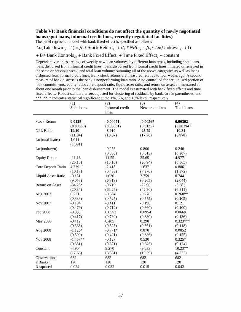
37
Table VI: Bank financial conditions do not affect the quantity of newly negotiated loans (spot loans, informal credit lines, recently negotiated facilities) The panel regression model with bank fixed-effect is specified as follows:
constantEffect Fixed TimeEffect FixedBank ControlsBank
)1Undrawn(*ReturnStock )1Takedown(
,
,3,2,1,
titi
titititi LnNPLLn
Dependent variables are logs of weekly new loan volumes, by different loan types, including spot loans, loans disbursed from informal credit lines, loans disbursed from formal credit lines initiated or renewed in the same or previous week, and total loan volumes summing all of the above categories as well as loans disbursed from formal credit lines. Bank stock returns are measured relative to four weeks ago. A second measure of bank distress is the bank’s nonperforming loan ratio. Also controlled for are, unused portion of loan commitments, equity ratio, core deposit ratio, liquid asset ratio, and return on asset, all measured at about one month prior to the loan disbursement. The model is estimated with bank fixed effects and time fixed effects. Robust standard errors adjusted for clustering of residuals by banks are in parentheses, and ***, **, * indicates statistical significant at the 1%, 5%, and 10% level, respectively (1) (2) (3) (4) Spot loans Informal credit
lines New credit lines Total loans
Stock Return 0.0128 -0.00471 -0.00567 0.00302 (0.00860) (0.00881) (0.0135) (0.00294) NPL Ratio 19.10 -8.910 -25.79 -10.84 (11.94) (18.87) (17.28) (6.970) Ln (total loans) 1.011 (1.091) Ln (undrawn) -0.256 0.800 0.240 (0.365) (0.613) (0.207) Equity Ratio -11.16 11.55 25.65 4.977 (25.18) (16.16) (26.94) (5.363) Core Deposit Ratio 4.779 -2.413 1.637 0.886 (10.17) (6.488) (7.270) (1.372) Liquid Asset Ratio -9.151 1.626 2.759 0.744 (9.058) (6.319) (6.205) (2.044) Return on Asset -34.28* -0.719 -22.90 -3.582 (20.34) (66.27) (42.90) (6.311) Aug 2007 0.221 -0.694 -0.278 0.268** (0.383) (0.525) (0.575) (0.105) Nov 2007 -0.194 -0.411 -0.190 0.121 (0.479) (0.712) (0.660) (0.100) Feb 2008 -0.330 0.0552 0.0954 0.0669 (0.417) (0.730) (0.630) (0.136) May 2008 -0.412 0.405 0.290 0.323*** (0.568) (0.523) (0.561) (0.118) Aug 2008 -1.126* -0.771* 0.870 0.0852 (0.590) (0.421) (0.686) (0.155) Nov 2008 -1.457** -0.127 0.530 0.325* (0.631) (0.621) (0.645) (0.174) Constant -4.904 9.270 -9.633 10.23** (17.68) (8.581) (13.39) (4.222) Observations 682 682 682 682 # Banks 120 120 120 120 R-squared 0.024 0.022 0.015 0.042

38
Table VII: Information on individual loans Panel A: Interest rate and loan size The loan level data are from the Survey of Terms of Business Lending (STBL). Nominal interest rate is the compounded annual (360 days) interest rate charged on a loan. Credit spread is the nominal interest rate over the yield on treasury securities of similar repricing intervals. Loan size is the value of the loan disbursement. Commitment is the size of the credit limit on a credit line facility.
N Mean S.Dev. 25th Median 75th 95th Precommitted Formal Lines Nominal interest rate 177,017 6.24 1.78 4.92 6.00 7.58 9.25 Credit spread 177,017 3.73 1.14 3.01 3.75 4.34 5.66 Loan size ($000) 177,017 353 3,122 16 43 148 1,014 Commitment ($000) 177,017 8,551 235,719 500 2,000 7,000 30,000 New Formal Lines Nominal interest rate 12,340 6.67 1.78 5.25 6.50 8.00 9.50 Credit spread 12,340 4.09 1.28 3.33 3.95 4.83 6.25 Loan size ($000) 12,340 724 3,485 22 61 225 2,964 Commitment ($000) 12,340 5,448 113,925 96 500 3,000 20,000 Informal Lines Nominal interest rate 11,006 6.54 1.73 5.00 6.50 8.00 9.25 Credit spread 11,006 3.88 1.12 3.31 3.87 4.47 5.57 Loan size ($000) 11,006 146 697 13 30 91 450 Commitment ($000) 11,006 3,460 7,822 400 1,400 4,000 14,286 Spot Loans Nominal interest rate 12,491 7.10 1.89 6.00 7.00 8.25 10.25 Credit spread 12,491 4.19 1.60 3.28 4.04 5.18 6.58 Loan size ($000) 12,491 974 6,893 12 30 122 2,500
Panel B: Loan characteristics by categories
Share of total Precommitted Formal Credit Lines
New Formal Credit Lines
Informal Credit Lines
Spot Loans
Secured Loans 0.82 0.77 0.90 0.79 Fixed Rate Loans 0.06 0.18 0.11 0.35 Maturity > 1 year 0.48 0.53 0.64 0.76 No stated maturity 0.22 0.15 0.45 0.33 Non-rated loans 0.02 0.03 0.03 0.13 Rating=1 0.01 0.02 0.02 0.02 Rating=2 0.06 0.07 0.06 0.15 Rating=3 0.33 0.37 0.29 0.42 Rating=4 0.24 0.26 0.21 0.17 Rating=5 0.06 0.07 0.10 0.02 Rating Missing 0.28 0.19 0.30 0.08
N 177,017 12,340 11,006 12,491
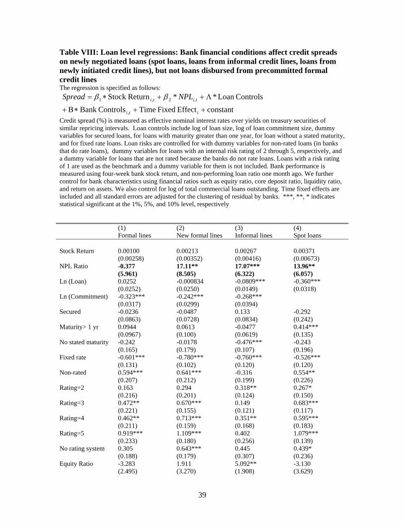
39
Table VIII: Loan level regressions: Bank financial conditions affect credit spreads on newly negotiated loans (spot loans, loans from informal credit lines, loans from newly initiated credit lines), but not loans disbursed from precommitted formal credit lines The regression is specified as follows:
constantEffect Fixed TimeControlsBank
ControlsLoan **ReturnStock
,
,2,1
iti
titi NPLSpread
Credit spread (%) is measured as effective nominal interest rates over yields on treasury securities of similar repricing intervals. Loan controls include log of loan size, log of loan commitment size, dummy variables for secured loans, for loans with maturity greater than one year, for loan without a stated maturity, and for fixed rate loans. Loan risks are controlled for with dummy variables for non-rated loans (in banks that do rate loans), dummy variables for loans with an internal risk rating of 2 through 5, respectively, and a dummy variable for loans that are not rated because the banks do not rate loans. Loans with a risk rating of 1 are used as the benchmark and a dummy variable for them is not included. Bank performance is measured using four-week bank stock return, and non-performing loan ratio one month ago. We further control for bank characteristics using financial ratios such as equity ratio, core deposit ratio, liquidity ratio, and return on assets. We also control for log of total commercial loans outstanding. Time fixed effects are included and all standard errors are adjusted for the clustering of residual by banks. ***, **, * indicates statistical significant at the 1%, 5%, and 10% level, respectively (1) (2) (3) (4) Formal lines New formal lines Informal lines Spot loans Stock Return 0.00100 0.00213 0.00267 0.00371 (0.00258) (0.00352) (0.00416) (0.00673) NPL Ratio -0.377 17.11** 17.07*** 13.96** (5.961) (8.505) (6.322) (6.057) Ln (Loan) 0.0252 -0.000834 -0.0809*** -0.360*** (0.0252) (0.0250) (0.0149) (0.0318) Ln (Commitment) -0.323*** -0.242*** -0.268*** (0.0317) (0.0299) (0.0394) Secured -0.0236 -0.0487 0.133 -0.292 (0.0863) (0.0728) (0.0834) (0.242) Maturity> 1 yr 0.0944 0.0613 -0.0477 0.414*** (0.0967) (0.100) (0.0619) (0.135) No stated maturity -0.242 -0.0178 -0.476*** -0.243 (0.165) (0.179) (0.107) (0.196) Fixed rate -0.601*** -0.780*** -0.760*** -0.526*** (0.131) (0.102) (0.120) (0.120) Non-rated 0.594*** 0.641*** -0.316 0.554** (0.207) (0.212) (0.199) (0.226) Rating=2 0.163 0.294 0.318** 0.267* (0.216) (0.201) (0.124) (0.150) Rating=3 0.472** 0.670*** 0.149 0.683*** (0.221) (0.155) (0.121) (0.117) Rating=4 0.462** 0.713*** 0.351** 0.595*** (0.211) (0.159) (0.168) (0.183) Rating=5 0.919*** 1.109*** 0.402 1.079*** (0.233) (0.180) (0.256) (0.139) No rating system 0.305 0.643*** 0.445 0.439* (0.188) (0.179) (0.307) (0.236) Equity Ratio -3.283 1.911 5.092** -3.130 (2.495) (3.270) (1.908) (3.629)

40
Core Deposit Ratio 1.181 -0.160 -4.761*** 0.825 (0.743) (0.524) (1.225) (1.053) Liquid Asset Ratio -0.714 -0.253 -0.366 -1.602*** (0.600) (0.718) (1.274) (0.601) Return on Asset -5.352 8.243 -0.397 2.004 (3.229) (5.703) (6.571) (7.644) Ln (total loan) -0.0689* -0.0675* -0.149*** -0.0506 (0.0389) (0.0343) (0.0460) (0.0402) Aug 2007 -0.109** -0.158** 0.166 0.00379 (0.0419) (0.0761) (0.127) (0.151) Nov 2007 0.235*** 0.147* 0.297** 0.453*** (0.0456) (0.0831) (0.120) (0.0935) Feb 2008 0.243*** 0.0742 -0.100 0.443*** (0.0716) (0.129) (0.214) (0.146) May 2008 -0.0335 -0.163 -0.508** 0.248 (0.0896) (0.119) (0.242) (0.177) Aug 2008 -0.201* -0.406*** -0.722*** 0.00888 (0.119) (0.149) (0.205) (0.264) Nov 2008 0.537*** 0.260 0.0317 0.707*** (0.150) (0.206) (0.165) (0.223) Constant 8.631*** 7.522*** 12.85*** 8.170*** (0.950) (0.685) (1.210) (1.348) Observations 177,017 12,340 11,006 12,491 R-squared 0.332 0.273 0.424 0.310