Hours worked by General Practitioners (GPs) and waiting

times for primary care 1

Megha Swamia 2, Hugh Gravelleb, Anthony Scottc, Jenny Williamsd

aMelbourne Institute of Applied Economic and Social Research and Department of Economics,

University of Melbourne

bCentre for Health Economics, University of York, UK

cMelbourne Institute of Applied Economic and Social Research, University of Melbourne

dDepartment of Economics, University of Melbourne

Abstract:Waiting times are an important measure of access to health services. Delay in

receiving primary care can affect patient health and increase use of hospitals. One of the key

factors contributing to the rising concern about accessibility to primary care are the changing

workload patterns and labour supply of General Practitioners (GPs) with increasing proportions

of GPs working shorter hours. Examining the effect on access to primary care of labour supply

at the intensive margin (hours of work) is important since GP supply at the extensive margin is

inflexible in short to medium run. We investigate the effect of hours worked by general practi-

tioners (GPs) on waiting times for GP appointments using panel data on 3,561 GPs from first

seven waves (2008-2014) of the Medicine in Australia: Balancing Employment and Life (MA-

BEL) survey of Australian doctors. We use both GP fixed effects and instrumental variables to

allow for the possible endogeneity of hours worked due to both time-invariant and time-varying

unobserved factors that might be correlated with GPs labour supply and waiting times. We also

1The authors would like to thank Tamara Taylor, the MABEL Data Manager, for assistancewith the Survey data. This study used data from the MABEL longitudinal survey of doctorsconducted by the University of Melbourne and Monash University (the MABEL research team).Funding for MABEL comes from the National Health and Medical Research Council (HealthServices Research Grant: 2008-2011; and Centre for Research Excellence in Medical WorkforceDynamics: 2012-2016) with additional support from the Department of Health (in 2008) andHealth Workforce Australia (in 2013).The MABEL research team bears no responsibility forhow the data has been analysed, used or summarised in this study.

2Correspondence to: Faculty of Business and Economics (FBE), University of Melbourne, 111Barry Street, Carlton VIC 3053, Australia. E-mail: mswami@student.unimelb.edu.au

control for a rich set of individual GP characteristics, practice features and characteristics of the

practice location. Our results suggest that waiting times do respond to changes in hours worked

by GPs. An increase in the average hours worked by 10 percent would reduce average waiting

time for a patient by about 12 percent. These results are largely driven by female GPs, who

work much fewer hours than male GPs due to a significant negative effect of childbearing on

women labour supply. We also find that quality indicators such as qualifications and experience

are associated with higher waiting times, and GPs working in relatively affluent areas and those

in areas with higher GP density have lower waiting times.

Keywords: waiting times; primary care; labour supply; fixed-effects; Instrumental

Variable model; MABEL Survey

2

1 Background and Motivation

Health care services play an important role in the welfare of the population in a

country and hence timely access to health care is vital for welfare. In markets

for most goods and services, the money price acts as a rationing mechanism to

equilibrate demand and supply. However, in health care markets public or private

insurance means that consumers either face a zero or below market clearing price

and rationing occurs through waiting times (Martin and Smith, 1999). Therefore,

waiting times are an important measure of access to health care.

Primary health care is typically the first point of contact with the health care

system and plays an important role in the diagnosis and management of patients’

health problems. However, concerns about access to primary health care services

has been growing in many countries (Sarma et al., 2011). On one hand, demand

for primary health services is increasing due to changing health needs, increased

prevalence of chronic diseases and ageing populations. On the other hand, changes

in the workload patterns and supply of General Practitioners (GPs) have become

an important issue in many countries including Australia, Canada and United

States (Crossley et al., 2009; Kirch and Vernon, 2008; Sarma et al., 2011). Research

indicates that young doctors are working less than their predecessors (Sarma et al.,

2011) and there has been an overall decline in the hours of direct patient care

(Crossley et al., 2009). In Australia too, there has been a significant decline in the

proportion of GPs working more than 40 hours in direct patient care from 41.8%

in 2003-04 to 30.6% in 2013-14 (Britt et al., 2013). These reductions in hours

worked by doctors are primarily attributed to the increasing proportion of female

doctors, ageing of the medical workforce and a shift of preferences towards greater

work-life balance (Crossley et al., 2009; Joyce et al., 2006; Kirch and Vernon, 2008;

Shrestha and Joyce, 2011). However, there is currently very little understanding of

how these changes in the labour supply of doctors influence access to health services

1

in general and in particular, waiting times in primary care. This is important since

medical training is a lengthy and costly process, and there are licensing restrictions

on entry into the medical profession. This makes supply at the extensive margin

inflexible in the short to medium run. As a result, a decline in the hours worked

by GPs could reduce the supply of ‘effective full-time practitioners’ 3 (Joyce et al.,

2006). Hence, changes in hours of work can have important implications for access

to primary care services.

In this study, we investigate the extent to which GP hours worked affect

waiting times for appointments with GPs. We perform the analysis separately

for female and male GPs since within-gender analysis controls for unobservable

gender-differences in productivity and practice styles which might affect demand

for consultations and waiting times. Further, as in other labour markets, research

on medical workforce suggests that female doctors on average work fewer hours

than their male counterparts (Gravelle and Hole, 2007; Kalb et al., 2015).

To answer our research questions, we first provide a simple theoretical frame-

work. The empirical analyses use the Medicine in Australia: Balancing Employ-

ment and Life (MABEL) panel survey of Australian doctors. The MABEL survey

provides the opportunity to study the impact of hours worked on waiting times as

it has unique information on the workload - both waiting times and hours worked,

of individual doctors. It also has rich data on doctors’ personal characteristics,

postgraduate qualifications, location, practice settings and style, which are likely

to affect demand and hence waiting times (Campbell et al., 2005; Cheraghi-Sohi

et al., 2008; Gandhi et al., 1997; Gerard et al., 2008; Scott, 2000; Scott and Vick,

1999; Scott et al., 2003; Turner et al., 2007).

We use panel data methods to control for unobserved heterogeneity at the indi-

vidual level. This mitigates the risk of omitted variable bias due to time-invariant

3It refers to a modified count of doctors, equivalent to FTE (Full Time Equivalent) practi-tioners. (http://www.phcris.org.au/fastfacts/fact.php?id=4833)

2

unobserved GP characteristics that might be correlated with both labour supply

decisions of the GPs and the waiting times, for example a GP’s intrinsic moti-

vation and passion towards his/her work. We also employ instrumental variables

(IV) to account for any time-varying unobserved factors correlated with both hours

worked and waiting times, for example, changing complexity of patients. The IV

approach will also address the concern about possible reverse causality between

hours worked and waiting times, which could arise if GPs respond to high waiting

times by increasing the hours worked. Regressing waiting times on hours worked

without taking into account these potential sources of endogeneity, we would ex-

pect to find a positive correlation between hours worked and the error term, which

would bias the expected negative estimated effect of hours worked on waiting times

upwards towards zero.

We find that waiting times for appointments respond to hours worked by GPs:

an increase in the average hours worked by a GP of 10 percent would reduce

the average waiting time by about 12 percent. This is largely driven by female

GPs who work much fewer hours than their male counterparts. We also find that

waiting times are affected by demand side factors including GP’s quality attributes

such as education and experience, and the socioeconomic status of the area and

GP density.

The study makes several contributions to the existing literature. It is the

first study to directly examine the impact of doctors’ labour supply decisions

on waiting times in primary care, using rich MABEL survey which has unique

information on waiting times for individual doctors and their labour supply. We

use instrumental variable methods to address the issue of time-varying omitted

variables and potential reverse causality between waiting times and labour supply,

in addition to exploiting panel data techniques to control for endogeneity due to

unobserved heterogeneity at individual level and unobserved time-invariant factors.

3

Moreover, we study waiting time for the preferred doctor and hence take into

account the patient-doctor relationship and the availability of continuous care.

This is important because patients generally prefer to see the same or a familiar

GP overtime (Guthrie and Wyke, 2006; Nutting et al., 2003; Rubin et al., 2006;

Schers et al., 2002) and there is evidence that patients are willing to wait longer

to see their preferred doctor (Rubin et al., 2006; Turner et al., 2007).

Delays in receiving primary care are costly not only in terms of risk of dete-

rioration of patients’ health condition, but also in terms of increased hospital or

emergency department use. Given that countries like Australia and U.K. are im-

plementing programs to encourage general practices to extend the working hours

(Department of Health and Ageing - Medicare Australia, 11; Department of Hu-

man Services, 2015b; Department of Health and Prime Minister’s Office U.K.,

2013), and Spain is implementing policies to extend the working hours of its Na-

tional Health System (NHS) personnel (Luigi et al., 2013), our study provides

insights about the extent to which such policy interventions could be helpful in

combating waiting times and improving access to primary care.

1.1 Empirical evidence on waiting time elasticities

There is a considerable body of research on waiting times in the health economics

literature which recognises that waiting times are determined by the interaction of

demand for and supply of health services when money prices cannot adjust to clear

the market. The bulk of literature focuses on hospital (non-emergency elective)

waiting times (Cullis and Jones, 1986; Goddard et al., 1995; Gravelle et al., 2003;

Iversen, 1993; Lindsay and Feigenbaum, 1984; Martin and Smith, 1999), with the

majority of studies outlining models to examine the responsiveness of demand for

and supply of hospital care to waiting times or waiting lists, using both cross-

sectional and longitudinal data (Gravelle et al., 2003; Martin et al., 2003). These

4

studies suggests that demand for hospital care is negatively associated with waiting

times (although relatively inelastic with elasticity estimates less than -0.5 in most

studies) and the supply is positively associated with waiting times. However, in

most of the studies the supply side is modeled relatively simply and lacks important

supply side features, such as availability of health personnel - doctors and allied

health professionals, which are central to supply capacity. This is primarily due

to the lack of available information on resources used by health providers.

Waiting times for primary care are a policy concern in several OECD countries

including Australia, Canada, U.K. and Sweden (Siciliani et al., 2013) but much

less studied by economists. The existing literature on accessibility to primary care

does not focus on waiting times as a measure of accessibility and is primarily based

on patient surveys. The majority of these studies focus on variation in reported

access by patients’ demographic characteristics such as age, gender, location and

self-reported health (Kontopantelis et al., 2010; Muggah et al., 2014; Young et al.,

2000) and find that being female, older in age, living in urban areas and having

better self-reported health is positively associated with better access to primary

care. Very few studies have looked at waiting times in primary care and those that

do, find that income and private insurance lead to faster access to GP care (Roll

et al., 2012). However, all of these studies provide information only about the

demand side of the market and they are mostly cross-sectional in nature. Hence,

results only suggests associations.

Therefore, there is a paucity of research on how waiting times in primary care

are affected by supply side factors. This is crucial in designing policies necessary

to ensure timely access to GP services in the face of rising demand for primary

health care.

Section 2 describes the institutional background to Australian health care.

Section 3 sets out the conceptual framework used for empirical analyses, section 4

5

describes the data and section 5 the empirical analyses including the econometric

method and results. The study concludes with a discussion of the results.

2 Institutional Context: General Practitioners

in Australia

GPs are the most commonly accessed primary health service in Australia and act

as gatekeepers to specialist care. Eighty two percent of Australians consulted a

GP at least once in previous 12 months in 2013-14 and the figure was eighty one

percent in 2012-13 (ABS, 2014). GPs primarily work in private practices with

various ownership arrangements and operate on a fee-for-service basis. Medicare

Australia sets out fixed subsidies or rebates for a range of GP services in the

Medicare Benefit Schedule (MBS) and GPs are free to set the level of their fees at

or above the MBS rebate, which acts as a floor price. However, Medicare provides

financial incentives to GPs to charge equal to the rebate amount i.e. bulk-bill,

for Commonwealth Concession Card holders and children under 16 years of age

(Department of Human Services, 2015a) with higher incentives in regional, rural

and remote areas (Rural and Regional Health Australia, Department of Health,

2015), and in this case patients pay no out-of-pocket costs.

Overall, around eighty percent of GP services are bulk-billed in Australia

(MBS, 2014). However, practices have distinct business models and practice styles.

For example, large corporate practices usually have a high volume-low price busi-

ness model where they bulk-bill all or most of their patients and see a high volume

of patients with short consultations. This usually occurs in areas of low socio-

economic status where price elasticities are relatively higher. On the other hand,

practices may bulk-bill only a small proportion of their patients and see a lower

number of patients, usually in more affluent areas (Gravelle et al., 2013). Patients

6

are free to choose any general practice and can visit any GP of their choice as

there is no compulsory patient list or registration system.

There has been a steady decline in the number of general practices in Australia,

from 8,309 practices in 2000-01 to 7,035 in 2010-11, owing to increases in practice

sizes (Carne, 2013). As a result, more than 90% of GPs are now working in group

practices and the majority of practices are located in metro areas (Britt et al.,

2013). General practices are characterized by group practice comprising GPs,

practice nurses and allied health professionals, and most general practices provide

prevention and early intervention services like immunization, and diabetes and

mental health programs.

3 Conceptual Framework: A simple model of

waiting time and hours worked for a GP

To explain how labour supply decisions of a GP might affect waiting times we use

a simple demand and supply framework. The demand for consultations with a GP

can be written as4:

D = D(w, q;xd, εd) (1)

where w is the waiting time, q is a measure of GP’s quality, xd is a vector of

exogenous demand shifters - socioeconomic characteristics such as income, educa-

tion, health status, age-distribution, etc., of local population and it also includes

other exogenous factors such as availability of substitutes and measure of compe-

tition. εd is the unobserved error which captures the effect of unmeasured factors

4See Cheraghi-Sohi et al. (2008); Gandhi et al. (1997); Gerard et al. (2008); Gravelle et al.(2003); Martin et al. (2003); Scott (2000); Scott and Vick (1999); Scott et al. (2003); Turneret al. (2007) for related literature and theoretical models.

7

shifting demand.

The model assumes that the GP bulk-bills all patients who therefore face a

zero price. We believe that this assumption is reasonable, given the institutional

context of Australia and the fact that most (80.3 % in 2013-2014) GP services are

bulk-billed in Australia (MBS, 2014).

On the supply side we assume that all consultations with a GP have the same

length (exogenously determined) t. Hours worked per week by the GP is denoted

h and n is the number of consultations per week with the GP. The number of

hours worked is h = nt, assuming that GPs spend all their time in direct patient

care.

The waiting time is determined by the market clearing condition that demand

for consultations D(.) equals the number of consultations supplied by the GP n:

D(w, q;xd, εd) − n = 0, Dw < 0, Dq > 0 (2)

The equilibrium waiting time is thus

w = w(q, n;xd, εd) (3)

which is very similar to the waiting time equation specified in Gravelle et al.

(2003) and Martin et al. (2003). Waiting time will decrease with the number of

consultations and hence hours worked, and will increase with higher quality:

wn = −−1

Dw

=1

Dw

< 0 (4)

8

and

wq = −Dq

Dw

> 0 (5)

Assuming that the GP bulk-bills all patients and so gets a fixed Medicare rebate

m per patient, the GP’s revenue will depend on the number of consultations she

has. She incurs financial costs of practicing which is given by c(n, q;xc, εc) where xc

are observed factors such as wage rates for allied health and administrative staff

and εc is the unobserved component that affects costs. The GP has exogenous

non-work income y0. The GP utility is

u = u(y, h, xg, εg) (6)

where y = y0 +mn− c(n, q;xc, εc), xg denote GP’s personal characteristics such as

age, gender, children, etc., and εg is an unobserved preference shifter. GP chooses

her hours h = nt of work to satisfy

uh + uy[m

t− cn

1

t] = 0 (7)

or

uht+ uy[m− cn] = 0 (8)

and so the number of hours of work is:

h = h∗(m, t, q, xc, xq, εc, εg) (9)

9

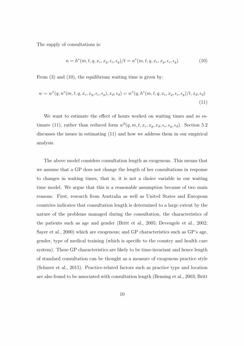
The supply of consultations is:

n = h∗(m, t, q, xc, xg, εc, εg)/t = n∗(m, t, q, xc, xg, εc, εg) (10)

From (3) and (10), the equilibrium waiting time is given by:

w = w∗(q, n∗(m, t, q, xc, xg, εc, εg), xd, εd) = w∗(q, h∗(m, t, q, xc, xg, εc, εg)/t, xd, εd)

(11)

We want to estimate the effect of hours worked on waiting times and so es-

timate (11), rather than reduced form w0(q,m, t, xc, xg, xd, εc, εg, εd). Section 5.2

discusses the issues in estimating (11) and how we address them in our empirical

analysis.

The above model considers consultation length as exogenous. This means that

we assume that a GP does not change the length of her consultations in response

to changes in waiting times, that is, it is not a choice variable in our waiting

time model. We argue that this is a reasonable assumption because of two main

reasons. First, research from Australia as well as United States and European

countries indicates that consultation length is determined to a large extent by the

nature of the problems managed during the consultation, the characteristics of

the patients such as age and gender (Britt et al., 2005; Deveugele et al., 2002;

Sayer et al., 2000) which are exogenous; and GP characteristics such as GP’s age,

gender, type of medical training (which is specific to the country and health care

system). These GP characteristics are likely to be time-invariant and hence length

of standard consultation can be thought as a measure of exogenous practice style

(Schurer et al., 2015). Practice-related factors such as practice type and location

are also found to be associated with consultation length (Bensing et al., 2003; Britt

10

et al., 2005; Deveugele et al., 2002). Our model incorporates all these factors.

Second, in Australia most general practices follow a fixed appointment scheduling

system where patients can book only 15-20 minutes’ appointments with the GPs

for a standard level B consultation5 6. In section 5, we test this assumption

empirically by using the number of patients (visits) seen (n in the model) instead

of hours worked as the main independent variable. n combines hours worked h

and consultation length t as per the theoretical model and we test whether using

n makes any qualitative difference to the results.

The model is a simple representation of the relationship between a GP’s hours

worked and waiting time and emphasizes the effect of GP’s labour supply decisions

on waiting time for consultation with her. Under reasonable assumptions the

model provides a framework for empirical examination of the effect of hours worked

on waiting times.

4 Data

We use data from the first seven waves (2008 to 2014) of the Medicine in Australia:

Balancing Employment and Life (MABEL) panel survey of Australian doctors.

The MABEL survey is tailored to four groups of clinicians - General Practitioners

(GPs), specialists, specialists in training and hospital non-specialists and provides

exceptionally rich data on these doctors’ workload, place of work, qualifications,

personal characteristics and family circumstances. The baseline 2008 cohort in-

cludes 10,498 Australian doctors including 3,906 GPs, 4,596 specialists, 1,072 spe-

cialists in training and 924 hospital non-specialists. The cohort was found to

5Level B consultation is defined as - Professional attendance involving taking a selectivehistory, examination of the patient with implementation of a management plan in relation to oneor more problems OR a professional attendance of less than 20 minutes duration (Britt et al.,2004)

6For evidence see: https://healthengine.com.au/

11

be nationally representative with respect to age, gender, geographic location and

hours worked. In the subsequent waves a new cohort of doctors was invited to par-

ticipate each year as a top-up sample. The methods of study and characteristics

of the baseline cohort are discussed in more detail in Joyce et al. (2010).

4.1 Waiting times and hours worked

Our dependent variable is the waiting time for an appointment with the GP in

the practice, in days. Each wave of the MABEL survey asks GPs to report on

three types of waiting times in their practice: ‘Excluding emergencies or urgent

needs, for how many days does a patient typically have to wait for (i) ’you’ their

preferred doctor in the practice (ii) any doctor in the practice, and (iii) waiting

time for a new patient in the practice? (please write average number of days)’.

For the analysis we use the responses to question (i) i.e. waiting time for ‘you’ the

preferred GP in the practice, since we are interested in examining the impact of a

GP’s labour supply decisions on his/her waiting time.

MABEL provides detailed information on the labour supply of doctors. In

addition to total hours worked, the doctors are asked to report the number of

hours worked in their most recent usual week at work in direct patient care, in-

direct patient care, educational activities, management and administration; and

also by various public and private settings - private medical practitioner’s rooms

or surgery, community health centre or other state-run primary care organization,

public and private hospital, residential/aged care health facility, aboriginal health

service, government department, tertiary education institution and others. Doc-

tors are also asked to report the number of patients they provided care in the most

recent usual week at work. On average GPs report spending most of their working

hours in private practice and in direct patient care (more than 80% of total hours

worked).

12

We use total hours worked as our measure of labour supply and use the infor-

mation on working hours from other questions to check for any reporting inconsis-

tencies (discussed in section 4.3). We believe that total hours is a better measure

of labour supply choice and is less likely to be measured with error. This is impor-

tant because we instrument for hours worked in our analysis using a set of family

characteristics and such instruments are likely to better explain the decision on

total hours. In a robustness check, we conduct our analysis using hours worked in

direct patient care per week to test whether it makes any qualitative difference to

the results.

4.2 Covariates

4.2.1 Personal characteristics

We use individual GP characteristics to control for factors that might influence

demand for consultations with the GP in the practice and hence waiting times.

We include GP’s standard consultation length (minutes per patient) as a proxy

for practice style. In the analysis with all GPs, we include GP gender as this

may affect the demand for their consultations, for example female patients might

prefer to see a female GP. Moreover, gender is also found to be associated with

labour supply decisions of doctors (Gravelle and Hole, 2007; Kalb et al., 2015).

We proxy for GP’s quality attributes using several variables. First, we include age

group, measured in five year bands, as a measure for GP’s experience 7. Second,

we include whether the GP is an Australian medical graduate, since graduating

from an Australian medical school (as opposed to an overseas school) may be

perceived by patients as higher quality. Third, we include whether the GP has a

7We also have information on ‘Years since graduation’ for each GP but it is not used becauseit will be perfectly collinear with year fixed effects for those GPs on which we have observationsfor consecutive years.

13

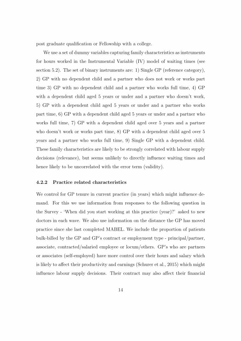
post graduate qualification or Fellowship with a college.

We use a set of dummy variables capturing family characteristics as instruments

for hours worked in the Instrumental Variable (IV) model of waiting times (see

section 5.2). The set of binary instruments are: 1) Single GP (reference category),

2) GP with no dependent child and a partner who does not work or works part

time 3) GP with no dependent child and a partner who works full time, 4) GP

with a dependent child aged 5 years or under and a partner who doesn’t work,

5) GP with a dependent child aged 5 years or under and a partner who works

part time, 6) GP with a dependent child aged 5 years or under and a partner who

works full time, 7) GP with a dependent child aged over 5 years and a partner

who doesn’t work or works part time, 8) GP with a dependent child aged over 5

years and a partner who works full time, 9) Single GP with a dependent child.

These family characteristics are likely to be strongly correlated with labour supply

decisions (relevance), but seems unlikely to directly influence waiting times and

hence likely to be uncorrelated with the error term (validity).

4.2.2 Practice related characteristics

We control for GP tenure in current practice (in years) which might influence de-

mand. For this we use information from responses to the following question in

the Survey - ‘When did you start working at this practice (year)?’ asked to new

doctors in each wave. We also use information on the distance the GP has moved

practice since she last completed MABEL. We include the proportion of patients

bulk-billed by the GP and GP’s contract or employment type - principal/partner,

associate, contracted/salaried employee or locum/others. GP’s who are partners

or associates (self-employed) have more control over their hours and salary which

is likely to affect their productivity and earnings (Schurer et al., 2015) which might

influence labour supply decisions. Their contract may also affect their financial

14

incentives and hence influence prices (Gravelle et al., 2013) and patient volume.

Further, being a principal/partner might also be associated by patients with se-

niority and higher quality. These are likely to affect the demand for GP in the

practice, and hence waiting times.

To allow for the effect of economies scale on practice costs and hence GP

productivity and efficiency (Damiani et al., 2013; Olsen et al., 2013; Reinhardt,

1972), we also control for size of the practice, measured by the total number of GPs

in the practice and also control for number of nurses, allied health professionals

and administrative staff in the practice.

4.2.3 Area measures

We include several GP practice postcode area level measures to capture factors

which may affect demand for primary care which is likely to be correlated with

both waiting times and hours worked. We control for the location of GP’s practice,

distinguishing between three categories based on Australian Standard Geographic

Classification (ASGC) of rurality: major city, regional (outer and inner) and re-

mote.

Patients’ socioeconomic status has been found to be negatively associated with

demand for primary care (Van Doorslaer et al., 2008; Van Doorslaer and Masse-

ria, 2004) and waiting times (Roll et al., 2012). It is also likely to affect price

elasticity of demand (Gravelle et al., 2013; Johar, 2012; Johar et al., 2014) and

this might influence practice’s choice of business model. We use Socio-Economic

Index for Areas (SEIFA) of Relative Socio-Economic Advantage and Disadvantage

constructed by Australian Bureau of Statistics census. It is based on measures of

income, education, occupational structure and employment status in a small area,

where higher values correspond to greater advantage. We match these to GPs on

the basis of their practice’s postcode.

15

We control for age distribution of the population in each postcode: the percent-

age of the population under 5 years of age and above 65 years of age, and distance

to nearest emergency department (in kilometers) as a measure of availability of

substitutes. We also include the number of GPs per 1000 population, at postcode

level8, as a measure of competition for GPs.

4.3 Analysis sample

The initial sample size of the unbalanced panel from seven waves of the Survey

for GPs is 24,609 observations on 6,707 GPs. Sample restrictions are used to take

into account inconsistencies and outliers. First, observations are excluded if the

difference between reported number of working hours across different questions in

the survey and total hours worked is greater than or equal to 5 hours9. Secondly,

to drop the outliers from the analysis, observations were not included if total hours

worked per week were less than 4 hours or greater than 75 hours a week10 or if

the waiting time for an appointment with the GP was reported to be greater than

30 days11. Similarly, other variables such as number of patients seen, standard

consultation length, number of GPs, nurses, allied health professionals and admin-

istrative staff, were checked for outliers and were coded missing correspondingly12.

The sample size with non-missing data on all variables of interest is 16,140 obser-

vations on 5,126 GPs. For the analysis, the sample was restricted to GPs with

8This data is based on Australian Medical Publishing Company (AMPCo) and 2011 Censusdata

9This was true in 1,058 cases or 4.5% of non-missing data on hours worked (23,612 observa-tions). This leaves 22,554 non-missing observations on hours worked.

10This was true in 1,011 cases or 4.48% of 22,554 observations.11This was true in 355 cases or 1.6% of 22,301 non-missing observations on waiting time.12‘Number of patients seen’ was coded missing if it was reported to be less than 10 or greater

than 300 per week; length of standard private consultation was coded missing if it was reportedto be less than 5 minutes or greater than 30 minutes; number of GPs was coded missing ifreported more than 30 GPs in practice; number of nurses, allied and administrative staff werecoded missing if reported greater than 30, 10 and 10 respectively.

16

at least two observations across seven waves, leaving 14,589 observations on 3,575

GPs in the estimation sample. Out of the 3,575 individual GP observations, 11%

are present in all seven waves, 15% each in six, five and four waves, 18% in three

waves and 26% in two waves.

5 Empirical Analysis

5.1 Descriptive analysis

Table 1 and 2 present the summary statistics of all variables for the analysis

sample. Half of GPs in the sample are females and aged 50 years or over. The

average waiting time for appointment with a GP is around 4 days, with female

GPs having higher average waiting time of 4.28 days compared to 3.76 days for

male GPs. Male GPs work 43.35 hours per week and female GPs works 31.64

hours per week on average, or about 73% of male weekly hours. Figures 1 and 2

show the distribution of waiting times and total hours worked. Most GPs have

waiting time less than 5 days, where male GPs have higher relative frequency of

zero waiting times (in days) as compared to their female counterparts (Figure 1).

Figure 2 reveals that female GPs work fewer hours than male GPs, with female GPs

working mostly work between 20 to 40 hours per week, while male GPs mostly

work between 35 to 55 hours per week. Moreover, the observed distribution of

hours worked indicates that for both part-time (less than 35 hours a week) and

full-time hours, ranges are fairly well covered.

On average female GPs have standard consultation length of 16.89 minutes,

about 14% longer than male GPs (14.76 minutes). Figure 3 shows the distribution

of consultation length. For both female and male GPs, the distribution is tight and

centered around 15 minutes, suggesting that most GPs spend around 15 minutes

per patient for a level B consultation.

17

Overall 74% of GPs are Australian medical graduates with 61% having post-

graduate degree or Fellowship of a college and mostly (67%) located in cities. Male

GPs bulk-bill a higher proportion of their patients, about 65%, as opposed to fe-

male GPs who bulk-bill about 56% of their patients13. Female GPs are more likely

to work in larger practices and as salaried/contracted employee. They are also

more likely work in areas with higher socio-economic status and GP density. Male

GPs are more likely to have a partner who is not working or working part time

and less likely to have dependent children aged under 5 years.

The standard deviations between GPs and within each GP over time indicates

the extent of variation in the sample. Overall the variation between different GPs

is larger than within a GP overtime, but there is still sufficient within variation

in waiting times and labour supply variables (columns 5-6 in Table 1 and columns

3-4 and 7-8 in Table 2). There is not much variation in consultation length, both

between and within GPs, with length of standard consultation varying less than 4

minutes between different GPs and less than 2 minutes for a GP over time (as also

suggested by the distribution of consultation length in Figure 3). This indicates

that our assumption of exogeneity of consultation length in the theoretical model

is reasonable, where most GPs have standard consultation length between 15-20

minutes for a standard level B consultation and a GP on average doesn’t change

his/her consultation length much over time.

For area level measures, the between variation is much larger than within vari-

ation, which is not surprising because area level measures are based on 2011 census

data and hence do not change overtime for an area (post code). Therefore, within

GP variation only results when a GP changes his workplace location (post code).

The between variation in family characteristics (instruments) is larger than

13It should be noted that the survey asks GPs to report proportion of patients bulk-billed,while the figure of 80% reported by (?) is based on the proportion of GP services (not patients)bulk-billed. A GP might to choose to bulk-bill some services and not bulk-bill others from thesame patient and hence the bulk-billing proportions reported in the survey are likely to be lower.

18

within variation, but there is still sufficient within variation. Figures 4 and 5

present the average hours worked for different family types for female and male

GPs. Overall, single GPs are not much different in their hours worked (both

total and direct patient care) from those having a partner but no dependent child,

irrespective of the employment status of the partner. For female GPs, having a

dependent child aged under 5 years and a partner who works seems to be associated

with significant reduction the average hours worked, with the reduction being

higher if partner works full time. Also, even if the dependent child is more than

5 years old, having a partner who works full time is associated with lower hours

worked. This indicates that, both having a young dependent child and employment

status of the partner are likely to play important role in labour supply decisions of

female GPs. For male GPs, there seems to be no significant relationship between

having a dependent child and employment status of the partner, and hours worked.

This suggests that our instruments are likely to work relatively better for female

GPs than for male GPs.

5.2 Econometric analysis

Based on the conceptual framework our baseline regression model is given by:

Wit = β0 + β1hit + β2Xit + λt + εit (12)

where Wit is the waiting time for GP i in year t, hit is the total hours worked; Xit

is a vector of control variables - GP characteristics, practice characteristics and

area level measures discussed in the section 4.2. λt is the year effect which controls

for shocks that affect waiting times for all GPs (cross-sectional dependence) such

as episodes of seasonal infections or an outbreak of some illness such as flu. We

19

estimate (12) for all GPs and separately by gender, using two types of models -

GP fixed effects and Instrumental Variable (IV), in addition to simple Ordinary

Least Squares (OLS) model.

5.2.1 GP fixed effects

The GP fixed effects model exploits the within-individual variation in both waiting

times and hours worked over the panel, mitigating endogeneity resulting from

the confounding effects of unobserved individual GP heterogeneity that might be

correlated with both waiting times and total hours worked. For example, a GP’s

intrinsic motivation and passion towards her work is likely to affect her choice of

hours and at the same time the demand for her consultations and hence waiting

times. This would result in endogeneity due to positive correlation between hit

and εit, biasing the estimates upwards (towards zero).

5.2.2 Instrumental Variables

As long as the omitted factors are time-invariant, such as GP’s interpersonal skills

and professional ethics which might affect quality and hence demand, GP fixed

effects model will remove the potential bias. However, if there are unobserved

omitted variables that are time-varying such as complexity of patients, then the

potential bias will not be removed by inclusion of GP fixed effects. We therefore

an employ instrumental variable approach to test and correct for this potential

endogeneity, using a set of binary variables capturing different family types to

instrument for hours worked. The IV approach will also address the potential

issue of reverse-causality between waiting times and hours worked which could

arise if GP’s change their hours in response to changes in waiting times.

We also estimate IV with GP fixed effects (FEIV) model. Although this model

will provide the most robust estimates since it mitigates the potential bias from

20

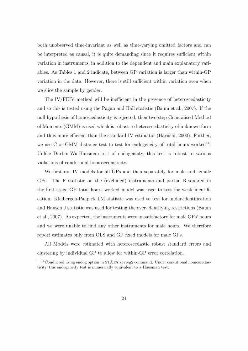
both unobserved time-invariant as well as time-varying omitted factors and can

be interpreted as causal, it is quite demanding since it requires sufficient within

variation in instruments, in addition to the dependent and main explanatory vari-

ables. As Tables 1 and 2 indicate, between GP variation is larger than within-GP

variation in the data. However, there is still sufficient within variation even when

we slice the sample by gender.

The IV/FEIV method will be inefficient in the presence of heteroscedasticity

and so this is tested using the Pagan and Hall statistic (Baum et al., 2007). If the

null hypothesis of homoscedasticity is rejected, then two-step Generalised Method

of Moments (GMM) is used which is robust to heteroscedasticity of unknown form

and thus more efficient than the standard IV estimator (Hayashi, 2000). Further,

we use C or GMM distance test to test for endogeneity of total hours worked14.

Unlike Durbin-Wu-Hausman test of endogeneity, this test is robust to various

violations of conditional homoscedasticity.

We first ran IV models for all GPs and then separately for male and female

GPs. The F statistic on the (excluded) instruments and partial R-squared in

the first stage GP total hours worked model was used to test for weak identifi-

cation. Kleibergen-Paap rk LM statistic was used to test for under-identification

and Hansen J statistic was used for testing the over-identifying restrictions (Baum

et al., 2007). As expected, the instruments were unsatisfactory for male GPs’ hours

and we were unable to find any other instruments for male hours. We therefore

report estimates only from OLS and GP fixed models for male GPs.

All Models were estimated with heteroscedastic robust standard errors and

clustering by individual GP to allow for within-GP error correlation.

14Conducted using endog option in STATA’s ivreg2 command. Under conditional homoscedas-ticity, this endogeneity test is numerically equivalent to a Hausman test.

21

5.3 Estimation results

5.3.1 Results for all GPs

Table 3 reports results from OLS, GP fixed effects, IV and FEIV models for all GPs.

The first column reports the OLS results. The coefficient on total hours worked

is positive and significant, indicating that higher hours worked is associated with

longer waiting times. As argued before, this is likely to be the result of strong

endogeneity of hours worked15. Once we control for GP fixed effects in column 2,

the coefficient becomes statistically insignificant16. However, the inclusion of GP

fixed effects corrects only for that part of the endogeneity problem that arises from

time-invariant individual GP heterogeneity. As discussed earlier, the total hours

worked is likely to be positively correlated with the error term due to time-varying

unobserved confounding factors and possible reverse-causality between total hours

worked and waiting times and this will bias the coefficient on hours towards zero.

To address these issues, we instrument for hours worked with a set eight binary

variables capturing different family types using single GP as the reference category

in columns 3 and 4. Once instrumented for, the effect of total hours worked

increases in magnitude and becomes negative. The IV model (column 3) exploits

the between-GP variation and results in a coefficient of -0.066 on total hours

worked, suggesting that an hour increase in total hours worked per week by a

GP is associated with a reduction in waiting times of about 32 minutes for an

appointment with the GP 17. The FEIV model exploits within-GP variation and

leads to a larger in magnitude effect with coefficient of -0.125 on total hours worked,

15This was tested using Durbin-Wu-Hausman test and it confirmed the endogeneity of hoursworked.

16The Hausman-Wu was applied and it rejected random effects in favour of the fixed effectsmodel with a p-value of 0.000, indicating a significant correlation between time-invariant omittedvariables and observed variables.

17We interpret the coefficients assuming 8 hours working day. So coefficient of -0.066 means areduction of 0.066 x 8 hours x 60 minutes = 31.68 minutes.

22

suggesting that an hour increase in total hours worked per week would reduce

waiting time for appointment with the GP by about 60 minutes. In terms of

elasticity, the FEIV model suggests that a 10 percent increase in average hours

worked by a GP would reduce the average waiting time by 11.7 percent.

The instruments work better in case of the IV model (F statistic = 41.09

(p < 0.000), partial R2 = 0.048), as compared to FEIV model (F statistic = 17.16

(p < 0.000), partial R2 = 0.018) given the larger between than within variation

in data, but they are still sufficiently strong in case of FEIV. Both IV and FEIV

models pass the under-identification and over-identifying restrictions tests18. The

C or GMM distance test of endogeneity confirmed the endogeneity of total hours

worked in both IV and FEIV models, with null hypothesis of exogeneity strongly

rejected at 1% level of significance. Table A1 in the appendix presents the results

of the first stage regression19. As expected, having a dependent child aged under

5 years is associated with a significant reduction in total hours worked, and this

negative effect is heightened by the presence of a partner who works full time.

Comparing results from OLS to GP fixed effects and IV models allows us to

identify the main source of endogeneity. When we move from OLS (column 1)

to IV (column 3) we eliminate the endogeneity bias resulting from time-varying

omitted factors and potential reverse-causality between total hours worked and

waiting times, and by doing so the hours worked coefficient becomes significantly

negative from significantly positive. On the other hand, when we only eliminate

bias caused by individual GP heterogeneity by using GP fixed effects (column 2),

the coefficient on hours worked becomes insignificant but remains positive. This

18The null hypothesis for Kleibergen-Paap rk LM test of under-identification is that equationis under-identified, which is rejected in our case with p < 0.000. For Hansen J test of over-identifying restrictions which is a test of validity of instruments, the null hypothesis is thatinstruments are valid and it is not rejected with p < 0.402 in case of IV and p < 0.376 in case ofFEIV.

19All appendix tables are available on request.

23

suggests that most of the endogeneity (positive correlation between total hours

worked and the error term) is resulting from time-varying unobserved confounding

factors and possible reverse-causality.

5.3.2 Results for Female GPs

Table 4 reports the results from OLS, GP fixed effects, IV and FEIV models for

female GPs. As expected, the instruments work well for female GPs. They are

stronger in case of IV model (F = 42.85, Partial R2 = 0.100) than in FEIV model

(F = 14.74, Partial R2 = 0.038), but are still satisfactory in FEIV model. Total

hours worked are found to be endogenous using both the C or GMM distance

test (P-values reported in Table 8) and Durbin-Wu-Hausman test (p < 0.000).

The hours worked get a negative coefficient of -0.042 in the IV model but not

statistically significant. The FEIV model results in a larger in magnitude and

significantly negative effect of total hours worked on waiting times (coefficient of

-0.096), with estimate suggesting that an hour increase in total hours worked per

week would reduce waiting time for an appointment by about 46 minutes, or in

terms of elasticity, a 10 percent increase in average hours worked would reduce the

average waiting time by 7.1 percent. Table A2 in the appendix presents the results

of the first stage regression and it confirms that the negative effects of having a

dependent child on hours worked are primarily driven by female GPs. Having a

dependent child aged under 5 years and a partner who works full time is associated

with a reduction in female GP labour supply of about 13 hours a week as compared

to a single female GP without a young dependent child (column 1).

5.3.3 Results for Male GPs

For male GPs we do not find any significant negative effects of hours worked

on waiting times in GP fixed effects model (Table 5). Due to instruments be-

24

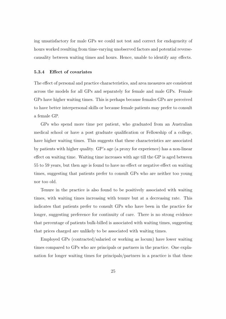
ing unsatisfactory for male GPs we could not test and correct for endogeneity of

hours worked resulting from time-varying unobserved factors and potential reverse-

causality between waiting times and hours. Hence, unable to identify any effects.

5.3.4 Effect of covariates

The effect of personal and practice characteristics, and area measures are consistent

across the models for all GPs and separately for female and male GPs. Female

GPs have higher waiting times. This is perhaps because females GPs are perceived

to have better interpersonal skills or because female patients may prefer to consult

a female GP.

GPs who spend more time per patient, who graduated from an Australian

medical school or have a post graduate qualification or Fellowship of a college,

have higher waiting times. This suggests that these characteristics are associated

by patients with higher quality. GP’s age (a proxy for experience) has a non-linear

effect on waiting time. Waiting time increases with age till the GP is aged between

55 to 59 years, but then age is found to have no effect or negative effect on waiting

times, suggesting that patients prefer to consult GPs who are neither too young

nor too old.

Tenure in the practice is also found to be positively associated with waiting

times, with waiting times increasing with tenure but at a decreasing rate. This

indicates that patients prefer to consult GPs who have been in the practice for

longer, suggesting preference for continuity of care. There is no strong evidence

that percentage of patients bulk-billed is associated with waiting times, suggesting

that prices charged are unlikely to be associated with waiting times.

Employed GPs (contracted/salaried or working as locum) have lower waiting

times compared to GPs who are principals or partners in the practice. One expla-

nation for longer waiting times for principals/partners in a practice is that these

25

GPs are considered as having higher quality and hence patients are willing to wait

more for such GPs. The coefficient on number of nurses is positive and signifi-

cant in several models, suggesting that practices with high waiting times might be

employing more nurses20.

Regional (for both female and male GPs) and remote (for female GPs) areas

have higher waiting times as compared to major cities. GPs in higher socioe-

conomic areas have lower waiting times which is consistent with what has been

found in the waiting time literature (Cooper et al., 2009; Laudicella et al., 2012;

Roll et al., 2012; Sharma et al., 2013; Siciliani and Verzulli, 2009; Sudano and

Baker, 2006). GPs in areas with higher proportion of elderly people have higher

waiting times, particularly female GPs, reflecting that elderly have higher demand

for primary health care. Waiting times are lower in areas with higher GP density,

suggesting a negative effect of competition on waiting times.

5.3.5 Sensitivity analyses

We carry out a number of sensitivity tests to investigate the robustness of the

results to alternative measures of GP’s labour supply and sample restrictions.

5.3.6 Alternative measure of labour supply

We estimated models with two separate measures of GP labour supply. First,

we use hours worked in direct patient care as the measure of labour supply to

test if that makes any qualitative difference to our results. Moreover, it allows us

to understand whether increase in hours spent in direct patient care and corre-

sponding decrease in hours spent in administrative and other activities can serve

as a means to lower waiting times without changing total hours worked. Second,

20This means that number of nurses are endogenous, but since it is a control variable in ourmodel and not our main independent variable, this does not affect our model and estimationstrategy.

26

to test the sensitivity of results to the assumption of exogeneity of consultation

length, we estimate models using number of patients (visits) seen per week as

the main explanatory variable. As per the theoretical model, number of patients

combines hours worked and consultation length into one variable and can be used

as an alternative measure of GP labour supply. If the assumption of exogenous

consultation length is reasonable then we should get qualitatively similar results21.

The results are reported in Table 6 and for brevity, only coefficient on hours

worked in direct patient care per week, and on number of patients seen per week

are reported. GP fixed effects model (column 2) results in negative and significant

(at 10% level) effect of hours worked in direct patient care for all GPs overall and

female GPs. The results of IV and FEIV models, however, remain qualitatively

similar for both all GPs and female GPs. The instruments are relatively weaker

for direct patient hours, particularly in FEIV model. As discussed before, this is

because our instruments capture family characteristics which are likely to explain

the choice of total hours worked relatively better than the hours spent in direct pa-

tient care, which might also be affected by other factors in the practice22. In case of

the IV model, the results indicate that hours spent in direct patient care are likely

to be associated with a relatively greater reduction in waiting times. It suggests

that spending more time in direct patient care and less time on administrative and

other work, can help reduce waiting times.

When we use ‘number of patients (visits) seen per week’ as the main explana-

tory variable in place of hours worked and consultation length, the instruments are

21We could not find any instrument for consultation length and hence could not formallytest for endogeneity. In this case, using number of patients seen as main explanatory variableprovides an alternative way to test the robustness of the results to the assumption of exogeneityof consultation length

22Both the C or GMM distance test and Durbin-Wu-Hausman test indicated that hours workedin direct patient care are endogenous at 5% level in case of all and female GPs, however, theP-values of both the test statistics were slightly larger as compared to those in case of total hoursworked.

27

satisfactory in case of IV model and we do get negative and significant coefficients

on number of patients seen. The estimates suggest that an extra patient seen per

week would be associated with reduction in waiting time of about 13 minutes for

all GPs overall and about 8 minutes for female GPs (column 3). Moreover, the fact

that our instruments based on family characteristics are satisfactorily explaining

number of patients seen by a GP (in IV model), indicates that consultation length

reflects practice style, i.e. longer versus shorter consultations, and hence the num-

ber of patients seen by a GP is likely to be proportional to hours worked. This

further shows that it is reasonable to assume consultation length to be exogenous

in our model.

5.3.7 Sample restrictions

In our theory model, we assumed that GP bulk-bills all patients. We therefore con-

duct our analysis only on GPs who bulk-bill 80 or more percent of their patients23.

The results are reported in Table 7 and for brevity, only coefficient on total hours

worked per week is reported. We still find negative and significant effect of total

hours worked on waiting times in case of IV model for all GPs and in addition,

find significantly negative (at 10% level) effect for female GPs. The magnitude of

the effects, however, is relatively large. In case of FEIV model, the instruments

become weak due to smaller sample size which reduces within variation in the data

and hence the estimates become imprecise.

Next, in order to test whether the results are not driven by GPs who are

principals/partners or associates in the practice who have greater control over

hours worked, we carry out the analysis separately for employed and self-employed

(principals/partners or associates) GPs. These results are also reported in Table

7. Overall the results remain qualitatively similar. However, as expected, the

23We did not use GPs who bulk-bill 100 percent of their patients because of very small samplesize to perform analysis.

28

estimates suggest that most of the endogeneity is driven by self-employed GPs.

This is possibly because GPs who are self-employed have much more control over

the hours they work and hence could alter their hours in response to unobserved

factors such as changing complexity of patients (which might also affect waiting

times). In case of all employed GPs, we still observe a negative and significant

effect of total hours worked on waiting times, although the magnitude of the effect

is slightly smaller. Due to small sample size of self-employed GPs, the instruments

become weak and hence the estimates becomes insignificant (in IV model) or less

significant (in FEIV model) due to loss of precision.

In case of female GPs, for those who are employed the negative effect of total

hours worked becomes statistically significant and increase in magnitude in IV

model. One possible explanation for finding stronger effect among employed female

GPs is that these female GPs have less control over their hours which prevents them

from flexibly adjusting their working hours to changes in exogenous circumstances

such as having a dependent child or spouse’s employment status and hence they are

more likely to reduce the hours worked in response to such external shocks. The

IV model is therefore able to identify the effects better for these employed female

GPs. In FEIV model, the coefficient remains negative but becomes insignificant

and the endogeneity test could not reject the null of exogeneity (P-value=0.140).

Hence, IV estimates are preferred. For self-employed female GPs, the sample size

is much smaller and hence most of the estimates are insignificant.

6 Discussion and conclusions

The labour supply of GPs is crucial to addressing the concerns about accessibility

to primary care services. This study examines the extent to which increasing the

labour supply at the intensive margin can reduce waiting times for appointments

29

with GPs using data from a unique Australian longitudinal survey of doctors. The

results suggest that, taking into account important demand side factors, waiting

times do respond negatively to hours worked by GPs: an increase in the average

hours worked by a GP by 10 percent would reduce average waiting time for a

patient by about 12 percent. These results are largely driven by female GPs where

our instruments are stronger.

Female GPs have longer waiting times, work shorter hours (31.64 per week

against male hours of 43.35 per week) and having dependent children significantly

reduces their labour supply at the intensive margin. On the other hand, male GPs

already work long hours and research indicates that male GPs have higher incomes

and negative wage elasticities of labour supply (Gravelle et al., 2011; Kalb et al.,

2015). Hence, it hard to provide incentives to male GPs to increase their hours

worked. Moreover, a recent study on Australian GPs found that male GPs do

not significantly alter their labour supply in response to having children (Schurer

et al., 2015). And this is the reason that we also find that family characteristics

could not satisfactorily serve as instruments for male GPs. Therefore, we are not

able to identify any significant effect of total hours worked on waiting times for

male GPs.

We find important evidence that waiting times for GPs are positively associated

with his/her quality attributes such being Australian trained, having post-graduate

qualification or Fellowship and experience, and by GP’s tenure in the practice and

employment status (principal/partner versus contracted/salaried employee). This

suggests that patients are willing to wait longer for a GP they perceive as a better

quality doctor. We also find that waiting times are lower in more affluent areas

and in areas with more competition as measured by GP density.

From policy perspective the findings of this study are important. With an

increased proportion of women in the medical workforce - the proportion of GPs

30

who are women increased from 36.5% in 2004 to 41.0% in 2014 (AIWH, 2015),

reduced labour supply by female GPs is likely to negatively affect the accessibility

to primary care services. Therefore, policy responses aimed at reducing average

waiting times in short to medium run by focusing on the intensive margin should

acknowledge the important role of female GPs and address ways of reducing the

negative effect of child-bearing on female GP labour supply. For example, by

improving child care policies and facilities for female doctors which provide them

with more flexibility in the hours they have to work enabling them to achieve

better work-life balance.

31

Table 1: Summary statistics of main variables and instruments for All GPs (N=14,544,n=3,561)

Overall S D S D

Variable Mean S D Min Max Between Within(1) (2) (3) (4) (5) (6)

Waiting time for you in practice 4.02 5.60 0 30 4.99 2.72Total hours worked per week 37.54 13.60 4 75 12.53 5.26Hours worked in direct patient care per week 31.18 12.18 4 75 11.24 4.93No. of patients (visits) seen per week 110.50 57.02 10 300 52.74 23.01

Personal characteristicsFemale 0.50 0.50 0 1 0.50 0.00Age: Under 35 0.09 0.28 0 1 0.30 0.12Age: 35-39 0.11 0.31 0 1 0.27 0.18Age: 40-44 0.12 0.33 0 1 0.26 0.21Age: 45-49 0.16 0.36 0 1 0.28 0.24Age: 50-54 0.18 0.38 0 1 0.29 0.26Age: 55-59 0.16 0.36 0 1 0.27 0.24Age: 60-64 0.10 0.30 0 1 0.23 0.20Age: 65 or over 0.09 0.29 0 1 0.27 0.12Length of std. private consultation 15.82 3.99 5 30 3.61 1.88Australian medical graduate 0.74 0.44 0 1 0.45 0.00Have post graduate qualification/Fellowship 0.61 0.49 0 1 0.46 0.16

Practice characteristicsTenure in practice (years) 9.00 9.81 0 61 9.16 3.21Total no. of GPs in the practice 7.76 4.17 1 25 3.82 1.92% of patients bulk-billed 60.56 30.15 0 100 27.78 12.29No. of nurses in the practice 2.39 1.90 0 10 1.70 0.92No. of allied health prof. & administrative staff in practice 6.18 4.20 0 30 3.59 2.38Employment type: Principal or partner 0.28 0.45 0 1 0.41 0.18Employment type: Associate 0.11 0.31 0 1 0.24 0.19Employment type: Salaried or Contracted employee 0.57 0.50 0 1 0.44 0.23Employment type: Locum or other 0.04 0.20 0 1 0.15 0.13

Area characteristicsLocation (ASGC): City 0.67 0.47 0 1 0.46 0.13Location (ASGC): Regional 0.31 0.46 0 1 0.45 0.13Location (ASGC): Remote 0.03 0.17 0 1 0.16 0.05SEIFA Index 1016.09 74.44 669.50 1213.92 70.92 23.26Percent of population under 5 yrs of age 6.03 1.40 0.43 13.34 1.32 0.52Percent of population above 65 yrs of age 13.89 4.96 0.18 43.37 4.71 1.67Min. distance to emergency department 4.62 3.53 1 19 3.29 1.29Ratio of GPs to population (per 1,000) 1.40 0.83 0.07 10.10 0.72 0.39

InstrumentsSingle 0.08 0.28 0 1 0.24 0.14No dep. child, partner doesn’t work or works part time 0.19 0.39 0 1 0.34 0.19No dep. child, partner works full time 0.11 0.32 0 1 0.28 0.18Dep. child ≤ 5 yrs, partner doesn’t work 0.03 0.16 0 1 0.13 0.10Dep. child ≤ 5 yrs, partner works part time 0.03 0.16 0 1 0.12 0.11Dep. child ≤ 5 yrs, partner works full time 0.05 0.21 0 1 0.17 0.12Dep. child > 5 yrs, partner doesn’t work or works part time 0.25 0.43 0 1 0.37 0.24Dep. child > 5 yrs, partner works full time 0.22 0.42 0 1 0.36 0.23Single, Dep. child 0.04 0.19 0 1 0.16 0.10

32

Table 2: Summary statistics of main variables and instruments by gender

Female GPs Male GPs(N=7,211, n=1,786) (N=7,333, n=1,775)

Variable Mean S D S D S D Mean S D S D S DOverall Between Within Overall Between Within

(1) (2) (3) (4) (5) (6) (7) (8)

Waiting time for you in practice 4.28 5.55 4.80 2.83 3.76*** 5.64 5.16 2.61Total hours worked per week 31.64 12.20 11.18 5.11 43.35*** 12.35 11.21 5.40Hours worked in direct patient care per week 25.79 10.63 9.76 4.54 36.47*** 11.26 10.21 5.29No. of patients (visits) seen per week 85.38 45.41 41.13 20.37 135.21*** 56.47 51.95 25.33

Personal characteristicsAge: Under 35 0.12 0.33 0.34 0.14 0.05*** 0.22 0.23 0.10Age: 35-39 0.14 0.34 0.29 0.21 0.08*** 0.26 0.23 0.15Age: 40-44 0.15 0.36 0.28 0.23 0.10*** 0.29 0.24 0.19Age: 45-49 0.17 0.38 0.29 0.25 0.14*** 0.35 0.27 0.23Age: 50-54 0.18 0.38 0.28 0.26 0.18 0.39 0.29 0.26Age: 55-59 0.13 0.34 0.25 0.22 0.18*** 0.39 0.29 0.26Age: 60-64 0.08 0.26 0.20 0.17 0.13*** 0.33 0.25 0.22Age: 65 or over 0.03 0.18 0.16 0.09 0.14*** 0.35 0.33 0.14Length of std. private consultation 16.89 4.16 3.70 2.05 14.76*** 3.52 3.19 1.70Australian medical graduate 0.78 0.42 0.44 0.00 0.71*** 0.45 0.47 0.00Have post graduate qualification/Fellowship 0.64 0.48 0.45 0.18 0.58*** 0.49 0.47 0.15

Practice characteristicsTenure in practice (years) 7.02 7.82 7.17 2.73 10.94*** 11.09 10.46 3.62Total no. of GPs in the practice 7.99 4.02 3.69 1.86 7.53*** 4.30 3.94 1.97% of patients bulk-billed 56.10 30.51 27.84 12.89 64.94*** 29.15 27.12 11.67No. of nurses in the practice 2.34 1.86 1.65 0.93 2.45*** 1.94 1.76 0.90No. of allied health prof. & administrative staff in practice 6.26 4.10 3.45 2.36 6.09** 4.30 3.71 2.39Employment type: Principal or partner 0.16 0.36 0.33 0.15 0.41*** 0.49 0.44 0.21Employment type: Associate 0.09 0.29 0.22 0.18 0.12*** 0.32 0.26 0.19Employment type: Salaried or Contracted employee 0.71 0.45 0.39 0.23 0.43*** 0.50 0.45 0.23Employment type: Locum or other 0.04 0.19 0.14 0.14 0.04 0.20 0.17 0.12

Area characteristicsLocation: City 0.71 0.45 0.44 0.14 0.62*** 0.49 0.47 0.13Location: Regional 0.27 0.44 0.43 0.14 0.35*** 0.48 0.46 0.13Location: Remote 0.02 0.15 0.15 0.06 0.03*** 0.18 0.18 0.05SEIFA Index 1028.62 74.51 71.01 25.19 1003.77 72.29 68.86 21.19Percent of population under 5 yrs of age 5.98 1.42 1.34 0.56 6.08*** 1.37 1.29 0.48Percent of population above 65 yrs of age 13.52 4.78 4.47 1.78 14.26*** 5.10 4.90 1.55Min. distance to emergency department 4.62 3.44 3.16 1.37 4.62 3.62 3.41 1.19Ratio of GPs to population (per 1,000) 1.47 0.89 0.76 0.41 1.32*** 0.77 0.67 0.37

InstrumentsSingle 0.10 0.30 0.27 0.15 0.07*** 0.25 0.22 0.14No dep. child, partner doesn’t work or works part time 0.10 0.30 0.26 0.15 0.28*** 0.45 0.39 0.22No dep. child, partner works full time 0.14 0.35 0.31 0.20 0.08*** 0.28 0.23 0.17Dep. child ≤ 5 yrs, partner doesn’t work 0.02 0.12 0.09 0.08 0.04*** 0.19 0.16 0.12Dep. child ≤ 5 yrs, partner works part time 0.02 0.13 0.09 0.09 0.03*** 0.18 0.14 0.12Dep. child ≤ 5 yrs, partner works full time 0.08 0.28 0.23 0.16 0.01*** 0.10 0.07 0.07Dep. child > 5 yrs, partner doesn’t work or works part time 0.13 0.34 0.28 0.20 0.37*** 0.48 0.41 0.26Dep. child > 5 yrs, partner works full time 0.35 0.48 0.40 0.26 0.10*** 0.30 0.25 0.18Single, Dep. child 0.06 0.23 0.20 0.11 0.02*** 0.14 0.11 0.09

Notes: The Asterisks denote significant difference in means for male GPs as compared to female GPs based on t-test of equality of means. ***, **, *significant at 1%, 5% and 10% respectively.

33

Figure 1

Figure 2

Figure 3

34

Figure 4

Figure 5

35

Table 3: Regression results for all GPs

Dependent variable: Waiting time for ’you’ in practice (days)

(1) (2) (3) (4)Independent Variables OLS GP fixed effects IV FEIV

Total hours worked per week 0.012** 0.006 -0.066** -0.125***(0.005) (0.006) (0.026) (0.043)

Personal characteristicsFemale 0.872*** - 0.217 -

(0.172) (0.299)Age: 35-39 [Excl: Under 35 years] 0.618*** 0.293 0.499** 0.162

(0.202) (0.278) (0.228) (0.280)Age: 40-44 0.897*** 0.297 0.741*** 0.372

(0.232) (0.388) (0.267) (0.389)Age: 45-49 0.969*** 0.233 0.998*** 0.637

(0.226) (0.453) (0.246) (0.469)Age: 50-54 0.963*** 0.163 1.134*** 0.709

(0.225) (0.496) (0.246) (0.527)Age: 55-59 0.567** -0.293 0.751*** 0.319

(0.233) (0.547) (0.248) (0.588)Age: 60-64 0.427* -0.466 0.410 -0.106

(0.246) (0.602) (0.280) (0.628)Age: 65 or over 0.024 -0.783 -0.662 -0.900

(0.288) (0.695) (0.415) (0.711)Practice style: Length of std. private consultation (min) 0.153*** 0.096*** 0.253*** 0.081***

(0.015) (0.018) (0.020) (0.019)Australian medical graduate 1.176*** - 0.740*** -

(0.156) (0.171)Have post graduate qualification/Fellowship 0.716*** 0.557*** 0.698*** 0.454**

(0.128) (0.192) (0.162) (0.204)

Practice characteristicsTenure in practice (years) 0.158*** 0.136*** 0.180*** 0.149***

(0.017) (0.023) (0.021) (0.024)Tenure in practice (years) squared -0.003*** -0.003*** -0.004*** -0.003***

(0.001) (0.001) (0.001) (0.001)Total no. of GPs in the practice 0.036** 0.005 0.063** -0.004

(0.017) (0.020) (0.024) (0.021)% of patients bulk-billed 0.001 0.004 0.000 0.003

(0.002) (0.003) (0.003) (0.003)No. of nurses in the practice 0.164*** 0.115*** 0.226*** 0.117***

(0.037) (0.043) (0.054) (0.044)No. of allied health prof. & admin. staff in practice 0.003 -0.011 0.055*** -0.013

(0.012) (0.013) (0.021) (0.013)Business relationship: Associate [Excl: Principal or partner] -0.200 -0.120 -0.684** -0.403*

(0.183) (0.205) (0.333) (0.234)Business relationship: Salaried or Contracted employee -0.733*** -0.446** -1.706*** -0.866***

(0.162) (0.208) (0.304) (0.260)Business relationship: Locum or other -0.877*** -0.585** -2.102*** -1.024***

(0.208) (0.247) (0.390) (0.302)

Area level characteristicsLocation (ASGC): Regional [Excl: City] 1.800*** 1.623*** 1.937*** 1.730***

(0.174) (0.287) (0.215) (0.299)Location (ASGC): Remote 1.558*** 1.123** 2.188*** 1.516**

(0.423) (0.514) (0.647) (0.607)SEIFA Index -0.006*** -0.002 -0.010*** -0.003*

(0.001) (0.001) (0.001) (0.002)Percent of population under 5 yrs of age -0.053 -0.044 -0.037 -0.039

(0.047) (0.062) (0.063) (0.066)Percent of population above 65 yrs of age 0.058*** 0.047** 0.060*** 0.049**

(0.015) (0.024) (0.016) (0.025)Min. distance to emergency department -0.056*** -0.043* -0.088*** -0.057**

(0.018) (0.025) (0.024) (0.028)Ratio of GPs to population (per 1,000) -0.179** -0.111 -0.341*** -0.082

(0.070) (0.086) (0.091) (0.087)

Year fixed effects Yes Yes Yes YesGP fixed effects No Yes No Yes

Observations 14,544 14,544 14,544 14,544R-squared 0.185 0.031 0.164 -Number of GPs 3,561 3,561 3,561 3,561

First Stage statisticsF-stat of excluded instruments [P-value] 41.09 [0.000] 17.16 [0.000]Partial R-squared of excluded instruments 0.048 0.018Underidentification test P-value 0.000 0.000Hansen J overidentification test P-value 0.402 0.376Endogeneity test P-value 0.000 0.001

Notes: Robust and clustered (at individual level) standard errors in the parenthesis. Coefficients for year fixed effectsand constant are omitted. ***, **, * significant at 1%, 5% and 10% respectively.

36

Table 4: Regression results for female GPs

Dependent variable: Waiting time for ’you’ in practice (days)

(1) (2) (3) (4)Independent Variables OLS GP fixed effects IV FEIV

Total hours worked per week 0.015** 0.005 -0.042 -0.096**(0.007) (0.009) (0.026) (0.041)

Personal characteristicsAge: 35-39 [Excl: Under 35 years] 0.902*** 0.501 0.619** 0.284

(0.250) (0.356) (0.288) (0.358)Age: 40-44 0.964*** 0.245 0.593* 0.075

(0.286) (0.518) (0.337) (0.505)Age: 45-49 0.950*** -0.012 0.778** 0.049

(0.278) (0.614) (0.308) (0.611)Age: 50-54 0.977*** -0.168 0.877*** 0.015

(0.280) (0.686) (0.319) (0.697)Age: 55-59 0.663** -0.700 0.768** -0.409

(0.305) (0.766) (0.348) (0.785)Age: 60-64 0.425 -1.177 0.494 -1.116

(0.334) (0.858) (0.400) (0.867)Age: 65 or over 0.397 -1.142 -0.428 -1.463

(0.492) (1.036) (0.559) (1.022)Practice style: Length of std. private consultation (min) 0.195*** 0.130*** 0.294*** 0.124***

(0.020) (0.024) (0.027) (0.024)Australian medical graduate 1.157*** - 0.764*** -

(0.219) (0.232)Have post graduate qualification/Fellowship 0.875*** 0.863*** 0.819*** 0.662**

(0.172) (0.248) (0.223) (0.264)

Practice characteristicsTenure in practice (years) 0.227*** 0.187*** 0.246*** 0.184***

(0.027) (0.034) (0.037) (0.034)Tenure in practice (years) squared -0.005*** -0.005*** -0.005*** -0.005***

(0.001) (0.001) (0.001) (0.001)Total no. of GPs in the practice 0.029 -0.001 0.049 -0.010

(0.023) (0.027) (0.031) (0.028)% of patients bulk-billed 0.002 0.005 0.004 0.003

(0.003) (0.004) (0.004) (0.004)No. of nurses in the practice 0.169*** 0.144** 0.204*** 0.149**

(0.056) (0.066) (0.075) (0.066)No. of allied health prof. & admin. staff in practice 0.005 -0.011 0.063** -0.017

(0.018) (0.019) (0.028) (0.019)Business relationship: Associate [Excl: Principal or partner] -0.188 -0.150 -0.835 -0.336

(0.329) (0.368) (0.521) (0.387)Business relationship: Salaried or Contracted employee -0.789*** -0.581* -1.677*** -0.877**

(0.265) (0.329) (0.446) (0.367)Business relationship: Locum or other -1.192*** -1.010*** -2.119*** -1.332***

(0.321) (0.385) (0.561) (0.430)

Area level characteristicsLocation (ASGC): Regional [Excl: City] 1.660*** 1.576*** 1.773*** 1.694***

(0.251) (0.413) (0.297) (0.421)Location (ASGC): Remote 2.123*** 2.360*** 2.315*** 2.914***

(0.639) (0.719) (0.868) (0.755)SEIFA Index -0.007*** -0.002 -0.010*** -0.003

(0.001) (0.002) (0.002) (0.002)Percent of population under 5 yrs of age -0.031 -0.013 -0.019 -0.026

(0.063) (0.080) (0.092) (0.084)Percent of population above 65 yrs of age 0.070*** 0.062* 0.073*** 0.045

(0.022) (0.036) (0.023) (0.036)Min. distance to emergency department -0.034 -0.033 -0.040 -0.042

(0.027) (0.037) (0.034) (0.040)Ratio of GPs to population (per 1,000) -0.149 -0.048 -0.302** -0.053

(0.101) (0.128) (0.120) (0.129)

Year fixed effects Yes Yes Yes YesGP fixed effects No Yes No Yes

Observations 7,211 7,211 7,211 7,211R-squared 0.198 0.043 0.189 -Number of GPs 1,786 1,786 1,786 1,786

First Stage statisticsF-stat of excluded instruments [P-value] 42.85 [0.000] 14.74 [0.000]Partial R-squared of excluded instruments 0.100 0.038Underidentification test P-value 0.000 0.000Hansen J overidentification test P-value 0.416 0.393Endogeneity test P-value 0.007 0.009

Notes: Robust and clustered (at individual level) standard errors in the parenthesis. Coefficients for year fixedeffects and constant are omitted. ***, **, * significant at 1%, 5% and 10% respectively.

37

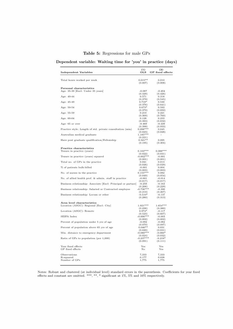
Table 5: Regressions for male GPs

Dependent variable: Waiting time for ’you’ in practice (days)

(1) (2)Independent Variables OLS GP fixed effects

Total hours worked per week 0.015** 0.010(0.007) (0.008)

Personal characteristicsAge: 35-39 [Excl: Under 35 years] -0.087 -0.204

(0.329) (0.426)Age: 40-44 0.571 0.318

(0.379) (0.545)Age: 45-49 0.718* 0.530

(0.376) (0.641)Age: 50-54 0.673* 0.593

(0.370) (0.692)Age: 55-59 0.210 0.221

(0.369) (0.760)Age: 60-64 0.128 0.233

(0.383) (0.832)Age: 65 or over -0.469 -0.229

(0.399) (0.933)Practice style: Length of std. private consultation (min) 0.098*** 0.045

(0.023) (0.028)Australian medical graduate 1.185*** -

(0.221)Have post graduate qualification/Fellowship 0.501** 0.095

(0.195) (0.304)

Practice characteristicsTenure in practice (years) 0.103*** 0.088***

(0.022) (0.031)Tenure in practice (years) squared -0.002*** -0.001

(0.001) (0.001)Total no. of GPs in the practice 0.041 0.013

(0.026) (0.029)% of patients bulk-billed -0.001 0.004

(0.003) (0.003)No. of nurses in the practice 0.155*** 0.082

(0.049) (0.054)No. of allied health prof. & admin. staff in practice -0.001 -0.014

(0.017) (0.017)Business relationship: Associate [Excl: Principal or partner] -0.259 -0.163

(0.206) (0.229)Business relationship: Salaried or Contracted employee -0.736*** -0.390

(0.210) (0.267)Business relationship: Locum or other -0.510* -0.137

(0.280) (0.313)

Area level characteristicsLocation (ASGC): Regional [Excl: City] 1.921*** 1.654***

(0.236) (0.380)Location (ASGC): Remote 0.974* -0.117

(0.523) (0.607)SEIFA Index -0.006*** -0.003

(0.002) (0.002)Percent of population under 5 yrs of age -0.092 -0.082

(0.070) (0.097)Percent of population above 65 yrs of age 0.046** 0.031

(0.020) (0.031)Min. distance to emergency department -0.080*** -0.060*

(0.024) (0.032)Ratio of GPs to population (per 1,000) -0.237*** -0.218*

(0.091) (0.111)

Year fixed effects Yes YesGP fixed effects No Yes

Observations 7,333 7,333R-squared 0.177 0.028Number of GPs 1,775 1,775

Notes: Robust and clustered (at individual level) standard errors in the parenthesis. Coefficients for year fixedeffects and constant are omitted. ***, **, * significant at 1%, 5% and 10% respectively.

38

Table 6: Results using ‘Hours worked in direct patient care per week’ and ‘No. ofpatients seen’ as measures of labour supply

Dependent variable: Waiting time for ’you’ in practice (days)

(1) (2) (3) (4)Main explanatory variable OLS GP fixed effects IV FEIV

ALL GPsHours worked in direct patient care per week -0.010* -0.011* -0.078** -0.196***

(0.005) (0.006) (0.032) (0.062)[F = 34.47] [F = 9.441]

No. of patients (visits) seen per week -0.005*** -0.001 -0.028*** -0.045**(0.001) (0.001) (0.010) (0.018)

[F = 15.44] [F = 6.428]

FEMALE GPsHours worked in direct patient care per week -0.010 -0.018* -0.046 -0.132**

(0.008) (0.010) (0.031) (0.054)[F = 40.61] [F = 11.43]

No. of patients (visits) seen per week -0.009*** -0.005** -0.017* -0.036**(0.002) (0.002) (0.010) (0.016)

[F = 23.91] [F= 8.104]

MALE GPsHours worked in direct patient care per week -0.006 -0.004 - -

(0.007) (0.008)

No. of patients (visits) seen per week -0.002 0.002 - -(0.001) (0.002)

Notes: The table only presents the coefficient on ‘hours worked in direct patient care per week’ and ‘no. ofpatients seen’ for the models for brevity. Complete tables are provided in the appendix. ***, **, * significantat 1%, 5% and 10% respectively.

39

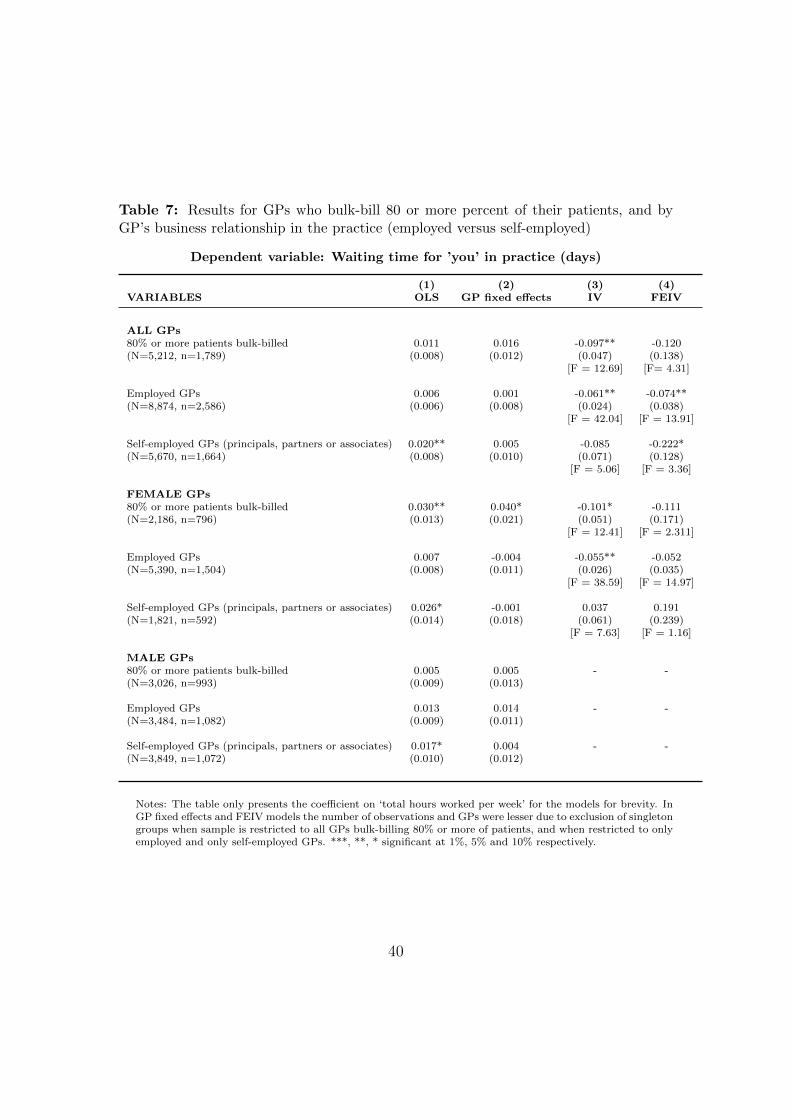
Table 7: Results for GPs who bulk-bill 80 or more percent of their patients, and byGP’s business relationship in the practice (employed versus self-employed)

Dependent variable: Waiting time for ’you’ in practice (days)

(1) (2) (3) (4)VARIABLES OLS GP fixed effects IV FEIV

ALL GPs80% or more patients bulk-billed 0.011 0.016 -0.097** -0.120(N=5,212, n=1,789) (0.008) (0.012) (0.047) (0.138)

[F = 12.69] [F= 4.31]

Employed GPs 0.006 0.001 -0.061** -0.074**(N=8,874, n=2,586) (0.006) (0.008) (0.024) (0.038)

[F = 42.04] [F = 13.91]

Self-employed GPs (principals, partners or associates) 0.020** 0.005 -0.085 -0.222*(N=5,670, n=1,664) (0.008) (0.010) (0.071) (0.128)

[F = 5.06] [F = 3.36]

FEMALE GPs80% or more patients bulk-billed 0.030** 0.040* -0.101* -0.111(N=2,186, n=796) (0.013) (0.021) (0.051) (0.171)

[F = 12.41] [F = 2.311]

Employed GPs 0.007 -0.004 -0.055** -0.052(N=5,390, n=1,504) (0.008) (0.011) (0.026) (0.035)

[F = 38.59] [F = 14.97]

Self-employed GPs (principals, partners or associates) 0.026* -0.001 0.037 0.191(N=1,821, n=592) (0.014) (0.018) (0.061) (0.239)

[F = 7.63] [F = 1.16]

MALE GPs80% or more patients bulk-billed 0.005 0.005 - -(N=3,026, n=993) (0.009) (0.013)

Employed GPs 0.013 0.014 - -(N=3,484, n=1,082) (0.009) (0.011)

Self-employed GPs (principals, partners or associates) 0.017* 0.004 - -(N=3,849, n=1,072) (0.010) (0.012)

Notes: The table only presents the coefficient on ‘total hours worked per week’ for the models for brevity. InGP fixed effects and FEIV models the number of observations and GPs were lesser due to exclusion of singletongroups when sample is restricted to all GPs bulk-billing 80% or more of patients, and when restricted to onlyemployed and only self-employed GPs. ***, **, * significant at 1%, 5% and 10% respectively.

40

References

ABS (2014). Patient Experiences in Australia: Summary of Findings, 2013

-14. http://www.abs.gov.au/ausstats/abs@.nsf/Lookup/by%20Subject/

4839.0~2013-14~Main%20Features~General%20practitioners~2.

AIWH (2015). Medical Practitioner workforce. Australian Institute of

Health and Welfare. http://www.aihw.gov.au/workforce/medical/

types-of-medical-practitioners/.

Baum, C. F., Schaffer, M. E., and Stillman, S. (2007). Enhanced routines for

instrumental variables/GMM estimation and testing. Stata Journal, 7(4):465 –

506.

Bensing, J. M., Roter, D. L., and Hulsman, R. L. (2003). Communication patterns

of primary care physicians in the United States and the Netherlands. Journal

of general internal medicine, 18(5):335 – 342.

Britt, H., Miller, G. C., Henderson, J., Bayram, C., Valenti, L., Harrison, C.,

Charles, J., Pan, Y., Zhang, C., and Pollack, A. (2013). A decade of Australian

general practice activity 2003-04 to 2012-13: General practice series no. 34,

volume 34. Sydney University Press.

Britt, H., Valenti, L., Miller, G. C., and Farmer, J. (2004). Determinants of GP

billing in Australia: content and time. Medical Journal of Australia, 181:100–

105.

Britt, H. C., Valenti, L., and Miller, G. C. (2005). Determinants of consultation

length in Australian general practice. Medical Journal of Australia, 183(2):68.

Campbell, J. L., Ramsay, J., Green, J., and Harvey, K. (2005). Forty-eight hour

41

access to primary care: practice factors predicting patients’ perceptions. Family

practice, 22(3):266–268.

Carne, A. (2013). Summary data report of the 2011-2012 annual survey of di-

visions of general practice. Report, Adelaide: Primary Health Care Research

& Information Service, Discipline of General Practice, Flinders University, and

Australian Government Department of Health and Ageing.

Cheraghi-Sohi, S., Hole, A. R., Mead, N., McDonald, R., Whalley, D., Bower, P.,

and Roland, M. (2008). What patients want from primary care consultations: a

discrete choice experiment to identify patients’ priorities. The Annals of Family

Medicine, 6(2):107–115.

Cooper, Z. N., McGuire, A., Jones, S., Le Grand, J., et al. (2009). Equity, waiting

times, and NHS reforms: retrospective study. British Medical Journal, 339.

Crossley, T. F., Hurley, J., and Jeon, S.-H. (2009). Physician labour supply in

Canada: a cohort analysis. Health economics, 18(4):437–456.

Cullis, J. G. and Jones, P. R. (1986). Rationing by waiting lists: an implication.

The American Economic Review, pages 250–256.

Damiani, G., Silvestrini, G., Federico, B., Cosentino, M., Marvulli, M., Tirabassi,

F., and Ricciardi, W. (2013). A systematic review on the effectiveness of group

versus single-handed practice. Health policy, 113(1):180–187.

Department of Health and Ageing - Medicare Australia (2010 - 11). Practice

Incentives Program: The Auditor General Audit Report - Performance Au-

dit. http://anao.gov.au/~/media/Uploads/Documents/2010%2011_audit_

report_no5.pdf.

42

Department of Health and Prime Minister’s Office U.K. (2013). Seven day, 8am -

8pm, GP access for hard working people. Press release.

Department of Human Services (2015a). Incentive payments to GPs who bulk bill

concessional patients and children aged under 16 years.

Department of Human Services (2015b). Practice Incentive Program - After Hours

Incentive.

Deveugele, M., Derese, A., van den Brink-Muinen, A., Bensing, J., and De Mae-

seneer, J. (2002). Consultation length in general practice: cross sectional study

in six European countries. British Medical Journal, 325(7362):472.

Gandhi, I., Parle, J., Greenfield, S., and Gould, S. (1997). A qualitative investi-

gation into why patients change their GPs. Family practice, 14(1):49–57.

Gerard, K., Salisbury, C., Street, D., Pope, C., and Baxter, H. (2008). Is fast

access to general practice all that should matter? A discrete choice experiment

of patients’ preferences. Journal of Health Services Research and Policy, 13(2):3

– 10.

Goddard, J., Malek, M., and Tavakoli, M. (1995). An economic model of the

market for hospital treatment for non-urgent conditions. Health Economics,

4(1):41–55.

Gravelle, H. and Hole, A. R. (2007). The work hours of GPs: survey of English

GPs. British journal of general practice, 57(535):96 – 100.

Gravelle, H., Hole, A. R., and Santos, R. (2011). Measuring and testing for gen-

der discrimination in physician pay: English family doctors. Journal of Health

Economics, 30(4):660–674.

43

Gravelle, H., Scott, A., Sivey, P. M., and Yong, J. (2013). Competition, prices and

quality in the market for physician consultations. Melbourne Institute Working

Paper No. 23/13.

Gravelle, H., Smith, P., and Xavier, A. (2003). Performance signals in the public

sector: the case of health care. Oxford Economic Papers, 55(1):81–103.

Guthrie, B. and Wyke, S. (2006). Personal continuity and access in UK general

practice: a qualitative study of general practitioners’ and patients’ perceptions

of when and how they matter. BMC Family Practice, 7(1):11.

Hayashi, F. (2000). Econometrics. 2000. Princeton University Press. Section,

1:60–69.

Iversen, T. (1993). A theory of hospital waiting lists. Journal of Health Economics,

12(1):55–71.

Johar, M. (2012). Do doctors charge high income patients more? Economics

Letters, 117(3):596–599.

Johar, M., Jones, G., and Savage, E. (2014). What explains the quality and price

of GP services? An investigation using linked survey and administrative data.

Health Economics, 23(9):1115 – 1133.

Joyce, C. M., McNeil, J. J., and Stoelwinder, J. U. (2006). More doctors, but

not enough: Australian medical workforce supply 2001-2012. Medical Journal

of Australia, 184(9):441.

Joyce, C. M., Scott, A., Jeon, S.-H., Humphreys, J., Kalb, G., Witt, J., and

Leahy, A. (2010). The ”Medicine in Australia: Balancing Employment and

Life (MABEL)” longitudinal survey-Protocol and baseline data for a prospective

44

cohort study of Australian doctors’ workforce participation. BMC health services

research, 10(50):1 – 10.

Kalb, G., Kuehnle, D., Scott, A., Cheng, T. C., and Jeon, S.-H. (2015). What Fac-

tors Affect Doctors’ Hours Decisions: Comparing Structural Discrete Choice and

Reduced-Form Approaches. Report, Melbourne Institute of Applied Economic

and Social Research, The University of Melbourne.

Kirch, D. G. and Vernon, D. J. (2008). Confronting the complexity of the physician

workforce equation. JAMA, 299(22):2680–2682. 10.1001/jama.299.22.2680.

Kontopantelis, E., Roland, M., and Reeves, D. (2010). Patient experience of access

to primary care: identification of predictors in a national patient survey. BMC

family practice, 11(1):61.

Laudicella, M., Siciliani, L., and Cookson, R. (2012). Waiting times and socioeco-

nomic status: evidence from England. Social Science & Medicine, 74(9):1331 –

1341.

Lindsay, C. M. and Feigenbaum, B. (1984). Rationing by waiting lists. The

American Economic Review, pages 404 – 417.

Luigi, S., Michael, B., and Valerie, M. (2013). OECD Health Policy Studies Wait-

ing Time Policies in the Health Sector: What Works? OECD Publishing.

Martin, S., Jacobs, R., Rice, N., and Smith, P. (2003). Waiting times for elective

surgery: A hospital based approach. Report, University of York, York.

Martin, S. and Smith, P. C. (1999). Rationing by waiting lists: an empirical

investigation. Journal of Public Economics, 71(1):141 – 164.

MBS (2014). Medicare Benefits Schedule-Medicare Statistics. https:

//www.health.gov.au/internet/main/publishing.nsf/Content/

45

34A89144DB4185EDCA257BF0001AFE29/$File/MBS%20Statistics%

20Financial%20Year%202013-14%20external%2020140718.pdf.

Muggah, E., Hogg, W., Dahrouge, S., Russell, G., Kristjansson, E., Muldoon, L.,

and Devlin, R. A. (2014). Patient-reported access to primary care in Ontario:

Effect of organizational characteristics. Canadian Family Physician, 60(1):e24

– e31.

Nutting, P. A., Goodwin, M. A., Flocke, S. A., Zyzanski, S. J., and Stange, K. C.

(2003). Continuity of primary care: to whom does it matter and when? The

Annals of Family Medicine, 1(3):149 – 155.

Olsen, K. R., Gyrd-Hansen, D., S Arensen, T. H. t. j., Kristensen, T., Vedsted, P.,

and Street, A. (2013). Organisational determinants of production and efficiency

in general practice: a population-based study. The European Journal of Health

Economics, 14(2):267 – 276.

Reinhardt, U. (1972). A production function for physician services. The Review

of Economics and Statistics, pages 55 – 66.

Roll, K., Stargardt, T., and Schreyogg, J. (2012). Effect of type of insurance and

income on waiting time for outpatient care. The Geneva Papers on Risk and

Insurance-Issues and Practice, 37(4):609 – 632.

Rubin, G., Bate, A., George, A., Shackley, P., and Hall, N. (2006). Preferences

for access to the GP: a discrete choice experiment. British Journal of General

Practice, 56(531):743 – 748.

Rural and Regional Health Australia, Department of Health (2015).

Higher Bulk Bill Incentives in Regional, Rural and Remote Areas.

http://www.ruralhealthaustralia.gov.au/internet/rha/publishing.

46

nsf/Content/Higher_Bulk_Bill_Incentives_in_Regional_Rural_and_

Remote_Areas-Tasmania_and_Metropolitan_Areas.

Sarma, S., Thind, A., and Chu, M.-K. (2011). Do new cohorts of family physicians

work less compared to their older predecessors? The evidence from Canada.

Social Science & Medicine, 72(12):2049 – 2058.

Sayer, G., Britt, H., Horn, F., Bhasale, A., McGeechan, K., Charles, J., Miller,

G., Hull, B., and Scahill, S. (2000). Measures of health and health care delivery

in general practice in Australia. General Practice Series 3. Cat. no. GEP 3.

Canberra: AIHW.

Schers, H., Webster, S., van den Hoogen, H., Avery, A., Grol, R., and van den

Bosch, W. (2002). Continuity of care in general practice: a survey of patients’

views. British Journal of General Practice, 52(479):459 – 462.

Schurer, S., Kuehnle, D., Scott, A., and Cheng, T. C. (2015). A man’s blessing

or a woman’s Curse? The family-earnings gap of doctors. Melbourne Institute

Working Paper.

Scott, A. (2000). Economics of general practice. Handbook of health economics,

1:1175 – 1200.

Scott, A. and Vick, S. (1999). Patients, Doctors and Contracts: An Application

of Principal-Agent Theory to the Doctor-Patient Relationship. Scottish journal

of political economy, 46(2):111 – 134.

Scott, A., Watson, M. S., and Ross, S. (2003). Eliciting preferences of the commu-

nity for out of hours care provided by general practitioners: a stated preference

discrete choice experiment. Social science and medicine, 56(4):803 – 814.

47

Sharma, A., Siciliani, L., and Harris, A. (2013). Waiting times and socioeconomic

status: Does sample selection matter? Economic Modelling, 33:659 – 667.

Shrestha, D. and Joyce, C. M. (2011). Aspects of work-life balance of Australian

general practitioners: determinants and possible consequences. Australian jour-

nal of primary health, 17(1):40 – 47.

Siciliani, L., Borowitz, M., and Moran, V. (2013). Waiting Time Policies in the

Health Sector: What Works? OECD Health Policy Studies. OECD Publishing.

Siciliani, L. and Verzulli, R. (2009). Waiting times and socioeconomic status among

elderly Europeans: evidence from SHARE. Health Economics, 18(11):1295 –

1306.

Sudano, J. J. and Baker, D. W. (2006). Explaining US racial/ethnic disparities in

health declines and mortality in late middle age: the roles of socioeconomic

status, health behaviors, and health insurance. Social Science & Medicine,

62(4):909 – 922.

Turner, D., Tarrant, C., Windridge, K., Bryan, S., Boulton, M., Freeman, G.,

and Baker, R. (2007). Do patients value continuity of care in general practice?

An investigation using stated preference discrete choice experiments. Journal of

Health Services Research and Policy, 12(3):132 – 137.

Van Doorslaer, E., Clarke, P., Savage, E., and Hall, J. (2008). Horizontal inequities

in Australia’s mixed public/private health care system. Health Policy, 86(1):97

– 108.

Van Doorslaer, E. and Masseria, C. (2004). Income-related inequality in the use of

medical care in 21 OECD countries. OECD Paris.

48

Young, A. F., Dobson, A. J., and Byles, J. E. (2000). Access and equity in the

provision of general practitioner services for women in Australia. Australian and

New Zealand Journal of Public Health, 24(5):474 – 480.

49