hot film surface heat flux measurement to an impinging air jet
TRANSCRIPT
High resolution hot film measurement of surface heat flux to an
impinging jet
Tadhg S. O’Donovan1, Tim Persoons2 & Darina B. Murray2
1School of Engineering and Physical Sciences, Heriot-Watt University,
Edinburgh EH14 4AS, United Kingdom
2Mechanical and Manufacturing Engineering, Trinity College Dublin,
Dublin 2, Ireland
Abstract
To investigate the complex coupling between surface heat transfer and local fluid velocity in
convective heat transfer, advanced techniques are required to measure the surface heat
flux at high spatial and temporal resolution. Several established flow velocity techniques
such as Laser Doppler Anemometry, Particle Image Velocimetry and Hot Wire Anemometry
can measure fluid velocities at high spatial resolution (micron) and have a high frequency
response (up to 100 kHz) characteristic. Equivalent advanced surface heat transfer
measurement techniques however are not available; even the latest advances in high speed
thermal imaging do not offer equivalent data capture rates. The current research presents a
method of measuring point surface heat flux at high temporal and spatial resolution. A hot
film that works in conjunction with a Constant Temperature Anemometer (CTA) is flush
mounted on a heated flat surface. The CTA maintains the hot film at a temperature slightly
elevated above the temperature of the surface and has a frequency response rate up to 100
kHz. To demonstrate the efficacy of the technique, a cooling impinging air jet is directed at
the heated surface and the power required to maintain the hot film temperature is related
to the local heat flux to the fluid air flow. The technique is validated experimentally using a
more established surface heat flux measurement technique. The thermal performance of
the sensor is also investigated numerically. It has been shown that, with some limitations,
the measurement technique accurately and with improved spatial and temporal resolution
measures the surface heat transfer to an impinging air jet for a wide range of experimental
parameters.

Nomenclature
A Area m2
D Jet diameter m
h Convective heat transfer coefficient W/(m2K)
I Current A
k Thermal conductivity W/(mK)
Nu Nusselt number, (hD/k) -
Pr Prandtl number -
q Heat W
q’’ Heat flux W/m2
R Resistance Ω
Re Reynolds number, (ρUD/μ) -
T Temperature K
U Jet exit velocity ms-1
V Voltage V
Subscripts
eff Effective
geo Geometric
Introduction
Advanced surface heat flux and fluid flow measurement techniques are required to further
the understanding of the complex coupling between local flow velocities and the adjacent
surface heat flux in convective heat transfer applications. Several fluid velocity
measurement techniques exist that can measure flow velocities in 3 dimensions and at high
spatial and temporal resolution. For example, Laser Doppler Anemometry (LDA) can
measure the speed of micron sized seeding particles in a fluid flow at a rate in excess of 100
kHz (Albrecht et al. [1]). Particle Image Velocimetry has also been developed to the stage
where it can measure a velocity flow field at a rate of 10 kHz and to micron level resolution
(Raffel et al. [2]). Even before the advent of laser flow measurement techniques Hot-Wire
Anemometry, as described by Bruun [3], was capable of measuring fluid velocities in the
MHz range with good spatial resolution (circa 100 micron).
Surface heat flux measurement technology has not kept pace with developments of fluid
velocity measurement techniques. Thermocouples, Thermochromic Liquid Crystals (TLCs)
and Infrared Thermal Imaging all measure temperature and when applied to a uniform wall
heat flux boundary condition the surface heat transfer coefficient can be calculated. Even
the state-of-the-art of these technologies is not comparable to standard flow measurement
technologies. Fine wire thermocouples have a maximum frequency response rate in the
region of 330 Hz (Ireland and Jones [4]); Thermochromic Liquid Crystals have a much lower
frequency response rate and a narrow operating temperature range (normally 5 to 15°C).
High speed infrared thermal imaging and pyrometry are the latest advancements in heat
transfer measurement technology and can measure surface temperatures in the kHz region.
Golibic et al. [5] has employed thermal imaging for a transient measure of surface heat flux
to a two phase flow. In this case however, the Biot number is high and the transients are
slow. For time varying signals due to turbulent flows, where the amplitude of the
fluctuations is low relative to the magnitude, simple energy balance equations are
insufficient for the calculation of the time varying surface heat flux signal.
The thickness, thermal conductivity and heat capacitance of the surface (usually a thin foil)
will all need to be considered in calculations of the surface heat flux. In the case of infrared
thermal imaging, high frequency imaging does not directly equate to high speed surface flux
measurements, no more than it does for surfaces coated in thermochromic liquid crystals. A
study by Nakamura [6] however, has shown that the maximum surface heat flux frequency
detectable using thermal imaging of very thin foils (2 to 10 microns) is still in the range of
100 Hz when used in air flows. While this falls short of what is available in fluid flow
measurements, this is a very useful advancement in the technology and is likely to aide
many convective heat transfer measurement investigations. A further disadvantage of the
heat transfer measurement technology discussed so far is their exclusive applicability to
uniform wall flux (UWF) surfaces. These technologies cannot be used for uniform wall
temperature conditions to calculate the surface heat flux.
To address the need for an accurate surface heat flux measurement technique with high
spatial and temporal resolution, the use of a flush mounted hot film for surface heat flux
measurement is under investigation. It is applied in an impinging jet flow as this is an
established area that would nevertheless benefit from the improvement in understanding
brought about by higher resolution data. Impinging jet flows are a very effective means of
achieving high rates of surface heat transfer. For this reason they are employed in several
heat transfer applications including turbine blade and electronics cooling.
An early study of jet impingement heat transfer was conducted by Hoogendoorn [7] where
the effect of jet exit turbulence on the stagnation point heat transfer is investigated. Gardon
and Akfirat [8] also conducted a study of the role of turbulence in jet impingement heat
transfer; both studies inferred the effect that velocity fluctuations had on the mean surface
heat transfer. Research in this area has been extensive and more recently the measurement
of surface heat transfer fluctuations to an impinging jet flow has given new insight into the
convective heat transfer mechanisms. Liu and Sullivan [9] used a hot film sensor to measure
time varying surface heat flux signal to an impinging air jet. While the technique used by Liu
and Sullivan [9] measured the magnitude of the surface heat flux fluctuations accurately,
the mean surface heat flux was measured by other means.
O’Donovan and Murray [10, 11] investigated the effect of vortices, that occur naturally in an
impinging jet flow, on the surface heat transfer for jets impinging at low nozzle to surface
spacings. By mounting a hot film on the impingement surface the time varying surface heat
flux signal was acquired but needed to be referenced to a separate measure of the mean
surface heat flux. This approach led to the finding that as vortices break down in the wall jet
the surface heat transfer is enhanced to form a secondary peak at a radial location.
The use of flush mounted hot film sensors to measure surface heat flux therefore is not
new. Xie and Wroblewski [12] used a hot film to study the time resolved heat flux
downstream of a cylinder-wall junction. Beasley and Figiola [13] developed a technique to
calibrate the sensor. It was found that the effective surface area of the sensor can vary from
1 to 10 times the geometric surface area depending on the operating parameters and the
magnitude of the surface heat flux. Moen and Schneider [14] investigated the frequency
response for a hot film sensor which is reported to be approximately 100 kHz for similar
nickel sensor elements. Moen and Schneider [14] also found that the frequency response
increased with larger values of sensor overheat.
Since a hot film must operate at a temperature above that of the surface, this sensor
overheat introduces an error in the surface heat flux signal. A correction for the sensor
overheat was first presented by Scholten and Murray [15] for a heated cylinder in cross-
flow. It was found that the technique is only valid for the attached flow regime within a
range from 0° (front stagnation point) to 100° (boundary layer separation point). As the
thermal performance of the sensor is still not fully understood it is not widely employed in
experimental investigations; an objective of the current research is to go some way towards
addressing this shortcoming.
Several investigators have used excitation techniques to further increase the localised and
area averaged heat transfer. Examples of such studies are those reported by Hwang et al.
[16] and Hwang and Cho [17]; an acoustic speaker was employed in these studies to control
the naturally occurring vortices within the flow. Excitation at a sub-harmonic of the natural
frequency for example, encouraged vortex merging and influenced the jet spread rate. This
in turn affected the surface heat transfer. Similar to earlier studies however, the influence of
the acoustic excitation on the resulting surface heat transfer is only inferred. Local and
temporally simultaneous velocity and surface heat transfer measurements at frequencies of
the same order of magnitude as the excitation frequencies would give greater insight into
the effect of the excitation of the surface heat transfer.
One of the most recent innovations in jet impingement cooling technology is synthetic air
jets. A jet is produced by the periodic oscillation of a membrane that forms one side of a
cavity; on the other side of the cavity is an orifice. Fluid is periodically drawn in and expelled
from the orifice and at certain formation criteria, defined by Smith and Glezer [18] and
Holman et al. [19], a jet is formed. The jet consists almost entirely of successive vortex rings
which can be directed at a heated surface to achieve a cooling effect. Because of the high
degree of turbulent mixing, synthetic jets have comparable performance to steady jets for
otherwise similar parameters (nozzle to impingement surface spacing, Reynolds number
etc.) Persoons et al. [20] have shown that synthetic jets perform similarly to the “bottom
end” of steady impinging jets issuing from a contoured nozzle. As this is a relatively new
technology it has yet to be optimised. Surface heat transfer measurements that can respond
to the activation frequencies of the synthetic air jet are required for this optimisation. It is
expected that this technology will need to be miniaturised to the micron scale and to
operate at high frequencies, in excess of 20 kHz (outside the human audible range) before it
will be suitable for many applications such as electronic cooling etc.
For these reasons, it is important that enhanced surface heat transfer techniques are
developed. New insight into convective heat transfer mechanisms in periodic and aperiodic
flows will lead to overall enhancement of cooling technology performance. The effect of
these techniques on the surface heat transfer can only be understood by analysing the
surface heat transfer at high spatial and temporal resolution. The use of a hot film that is
flush mounted on the heated impingement surface is investigated in the current research.
Although the response time of the sensor has the potential to improve the temporal
resolution for surface heat flux measurements, the current study is concerned with
measuring the time-average surface heat flux. The calibration of the sensor and details of
the measurement technique are presented.

Experimental Rig
The experimental rig is similar to that used in studies by O’Donovan and Murray [10, 11] and
is illustrated in figure 1. A 5mm thick copper plate is electrically heated from below and
approximates a uniform wall temperature boundary condition. Air is supplied to the jet
nozzle chamber though four separate inlets from the building compressors via a large
plenum chamber to eliminate flow fluctuations. Two filters are also connected on the
compressed air line to extract all trace of moisture and impurities from the air. An MKS mass
flow controller (model 1579A) is installed on the compressed air line to regulate the jet exit
Reynolds number. The meter is rated up to 300 litres/minute and has an accuracy of 1% of
full scale. The air flows though a dense mesh before exiting though the contoured nozzle
which forms a jet that is directed at the heated impingement surface. The 13mm diameter
jet is held above the heated surface in a clamp, the height of which can be varied from 0.5
to 10 jet diameters above the heated surface.
Figure 1: Experimental Test Rig
The heated impingement surface is instrumented with two flush mounted sensors. The first,
and the subject of this investigation, is a flush mounted hot film sensor supplied by Tao
Systems. The sensor consists of a nickel sensor element that is electron beam deposited
onto a 0.051mm thick Upilex S polyimide film. The hot film element has a thickness of <
0.2μm and covers an area of approximately 0.1mm x 1.4mm. Copper leads that have a
resistance of approximately 0.002Ω/mm are also deposited on the film to provide terminals
for connection to the constant temperature anemometer (CTA). A Dantec 90C10 Streamline
CTA module is used in the current investigation and the sensor is connected to the CTA with
a 1m long BNC cable. The hot film sensor element, together with the sensor cables form one
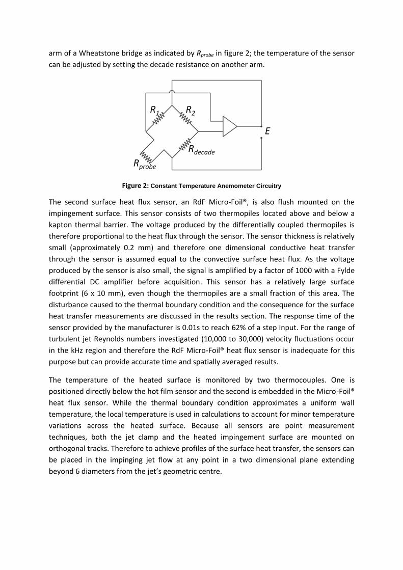
arm of a Wheatstone bridge as indicated by Rprobe in figure 2; the temperature of the sensor
can be adjusted by setting the decade resistance on another arm.
Figure 2: Constant Temperature Anemometer Circuitry
The second surface heat flux sensor, an RdF Micro-Foil®, is also flush mounted on the
impingement surface. This sensor consists of two thermopiles located above and below a
kapton thermal barrier. The voltage produced by the differentially coupled thermopiles is
therefore proportional to the heat flux through the sensor. The sensor thickness is relatively
small (approximately 0.2 mm) and therefore one dimensional conductive heat transfer
through the sensor is assumed equal to the convective surface heat flux. As the voltage
produced by the sensor is also small, the signal is amplified by a factor of 1000 with a Fylde
differential DC amplifier before acquisition. This sensor has a relatively large surface
footprint (6 x 10 mm), even though the thermopiles are a small fraction of this area. The
disturbance caused to the thermal boundary condition and the consequence for the surface
heat transfer measurements are discussed in the results section. The response time of the
sensor provided by the manufacturer is 0.01s to reach 62% of a step input. For the range of
turbulent jet Reynolds numbers investigated (10,000 to 30,000) velocity fluctuations occur
in the kHz region and therefore the RdF Micro-Foil® heat flux sensor is inadequate for this
purpose but can provide accurate time and spatially averaged results.
The temperature of the heated surface is monitored by two thermocouples. One is
positioned directly below the hot film sensor and the second is embedded in the Micro-Foil®
heat flux sensor. While the thermal boundary condition approximates a uniform wall
temperature, the local temperature is used in calculations to account for minor temperature
variations across the heated surface. Because all sensors are point measurement
techniques, both the jet clamp and the heated impingement surface are mounted on
orthogonal tracks. Therefore to achieve profiles of the surface heat transfer, the sensors can
be placed in the impinging jet flow at any point in a two dimensional plane extending
beyond 6 diameters from the jet’s geometric centre.
Theory
A CTA maintains the hot film sensor element at a constant resistance and hence a constant
sensor temperature. The sensor element is set to an elevated temperature above that of
the surrounding impingement surface. Hereafter this difference in temperature will be
referred to as the sensor overheat. The power required to maintain the sensor at this
temperature can be related to the surface heat flux. Ideally, to maintain a uniform wall
temperature boundary condition and to reduce errors associated with conductive losses etc,
the sensor would be maintained at a temperature equal to the heated surface. If this was
the case however, no power would be required to maintain its temperature as this would be
supplied from the heated surface. Therefore, to acquire a signal, it is necessary to overheat
the sensor. The influence of the sensor overheat magnitude on the surface heat flux
measurement is investigated in the current study. The power required to maintain the
sensor overheat temperature is equal to the heat losses from the sensor; these include
convective heat losses to the air flow and conduction to the heated surface. Therefore a
balance must be found, where the overheat is sufficiently large to produce a significant
signal (to maximise signal to noise ratio) but small enough so that errors can be easily
quantified and corrected for as part of the measurement technique.
The calibration of the hot film sensor technique for surface heat flux measurement has
many stages, the first of which is to determine the relationship between the film resistance
and film temperature. This is to ensure that the sensor overheat can be accurately
controlled using the decade resistance as part of the constant temperature anemometer.
The second part of the calibration procedure is to determine the effective surface area of
the sensor. The power, or heat dissipated from the film can be calculated from the
measurement of the voltage required to maintain the sensor at a certain temperature as
shown:
2IRq filmdissipated Equation 1
By balancing the Wheatstone bridge (figure 2), the current passing through the probe is
found to be:
probeRR
EI
1
Equation 2
and
cablefilmprobe RRR Equation 3
therefore
2
2
1
ERR
Rq
probe
film
dissipated Equation 4
Thus the dissipated heat from the sensor can be calculated from sensor properties and the
time-varying measurement of the CTA top bridge voltage.
Heat dissipated from the sensor element also conducts to the surrounding substrate and
sensor leads; this increases the effective surface area (Aeff) of the sensor. Therefore, in order
to calculate the surface heat flux the effective surface area must be calibrated against an
established reference heat flux measurement. There is a high degree of variability in the
heat transfer correlations for an impinging air jet. This is largely due to dissimilarities in the
jet flow characteristics. For otherwise similar experimental setups (i.e. Reynolds number,
nozzle to impingement surface spacing and thermal boundary condition) correlations by
Gardon and Akfirat [8] give very different results to those achieved by Goldstein and
Franchett [21] for example. The current setup is calibrated with reference to a correlation
(equation 55.04.0 RePr585.0Nu Equation 5)
developed by Liu and Sullivan [9] and based on a potential flow analysis by Shadlesky [22].
Equation 5 is valid for the surface heat transfer at the stagnation point, at low nozzle to
impingement surface spacings. It has been verified against experimental measurements by
Liu and Sullivan [9] for nozzle to impingement surface spacing less than 2 diameters and jet
exit Reynolds numbers from 12,000 to 15,000. This correlation was chosen as it was in good
agreement with the manufacturer’s independent calibration of the Micro-Foil® heat flux
sensor and also limits the experimental variables such as the effects of jet spread and the
entrainment of ambient fluids as it is only valid at the stagnation point and at nozzle to
impingement surface spacings that lie within the core of the jet.
5.04.0 RePr585.0Nu Equation 5
By combining equations 4 and 5 with Newton’s law of cooling, the effective surface area can
be calculated as:
5.04.02
1
2
RePr585.0 fluidjetsurfacecablefilm
film
effkTTRRR
DERA Equation 6
The above characterisation of the sensor effective surface area works only in ideal
circumstances where the sensor overheat is zero. As discussed earlier, in the absence of an
appreciable overheat the technique would not yield a measurement signal. It is therefore
necessary to apply a significant overheat to acquire a signal and then to correct for the
offset or bias error that the overheat introduces to the measurement signal. This third part
of the calibration procedure outlines the steps taken to measure the bias error to correct
the raw measurement.

Power dissipated from the sensor is a combination of convective heat transfer from the film
to the jet flow and conductive losses to the heated surface. Convective heat transfer is
overestimated as the temperature of the film is higher than the temperature of the
impingement surface surrounding the sensor. Heat is also conducted to the surface because
of the elevated hot film temperature. These factors contribute to a bias error in the raw
measurement. Both are difficult to estimate as the proportion of the bias error due to
convection requires foreknowledge of the convective heat transfer coefficient. And the
proportion of the bias error attributed to the conduction depends on precise measurements
of the sensor geometry and material properties. This can be further complicated by the use
of adhesives when mounting the sensor on the impingement surface. Therefore another
method is required to estimate the bias error before the surface heat flux can be accurately
established.
To accurately measure the bias error in the raw measurement, two tests are conducted. For
the same sensor overheat, jet positioning and Reynolds number, measurements are made
under heated and adiabatic conditions. In the heated test, the impingement surface is held
at a temperature above that of the ambient and impinging air jet. In the adiabatic test, the
impingement surface and jet air temperatures are maintained at ambient temperature. The
sensor, in both tests, is maintained at a constant overheat temperature above that of the
impingement surface and is located at the jet stagnation point.
For the adiabatic test, the sensor heat dissipation is equal to the sum of convection and
conduction from the sensor based on the overheat temperature difference as indicated in
equation 7:
OHTOHT convcondadiabatic qqq Equation 7
The heat flux from the sensor when the impingement surface is heated includes an
overestimate of the convection and conduction to the surface as indicated in 8:
airTsurfTOHTOHT convcondheated qqq Equation 8
Therefore, assuming the convective heat flux is linear with the temperature difference,
subtracting the dissipated heat from the sensor during adiabatic conditions from the
dissipated heat during heated conditions results in a measure of the surface heat flux based
on the temperature difference between the surface temperature and the jet temperature:
adiabaticheatedconv qqqairTsurfTT
Equation 9
In theory, therefore, this method can be applied for any overheat value. In practice
however, as will be discussed in the next session, it is still of benefit to minimise the
overheat as this, in turn, reduces the bias error and the disturbance of the thermal
boundary condition.
Results and Discussion
This section demonstrates the hot film surface heat flux measurement technique for an
impinging air jet. Firstly, the sensor calibration technique is analysed for the range of
parameters tested. This is then compared to a numerical simulation of the sensor’s thermal
performance. Finally, the results attained with the hot film technique are compared to those
determined by using a more established measurement technique.
Calibration of the Hot Film Sensor
As indicated in the experimental rig section, a thin unshielded T-type thermocouple in
embedded in the heated surface directly below the hot film sensor element. During
calibration a second thermocouple was positioned above the sensor element and the whole
system was insulated with fibreglass wool. The plate was then electrically heated to
approximately 100 degrees Celsius and allowed to cool slowly under the control of the
heating element; the apparatus was deemed to have reached a steady-state when the
temperature above and below the hot film fell within 0.1°C. At each temperature setting
the resistance of the hot film probe was measured by balancing the bridge with the decade
resistance. This ensured the probe was calibrated in situ while connected to the CTA. As
expected, a linear relationship was found between the probe resistance and temperature as
shown in equation 10:
000, 1 TTRR filmfilmfilm Equation 10
where the temperature coefficient of resistance α0 = 0.357 %/°C and the reference film
resistance, Rfilm,0 = 7.488Ω at a the reference temperature, T0 = 20°C
Both the uncertainty in the regression curve and the precision of the measurement is less
than 0.1% for the entire operating temperature range of the sensor. The probe resistance is
the sum of the film resistance and the resistance of the connecting cables. The cable
resistance was measured by shorting the lead terminals and balancing the Wheatstone
bridge; it was found to be 0.8Ω.
A series of tests were conducted where the hot film sensor was positioned at the stagnation
point of a jet impinging at a nozzle to impingement surface spacing of 2 diameters. The jet
Reynolds number was varied from 10000 to 30000 and the sensor overheat was also varied
from 3°C to 15°C.
2 4 6 8 10 12 14 165.4
5.5
5.6
5.7
5.8
5.9
6
6.1
6.2
Overheat, [ C]
Ae
ff/A
ge
om
etr
ic
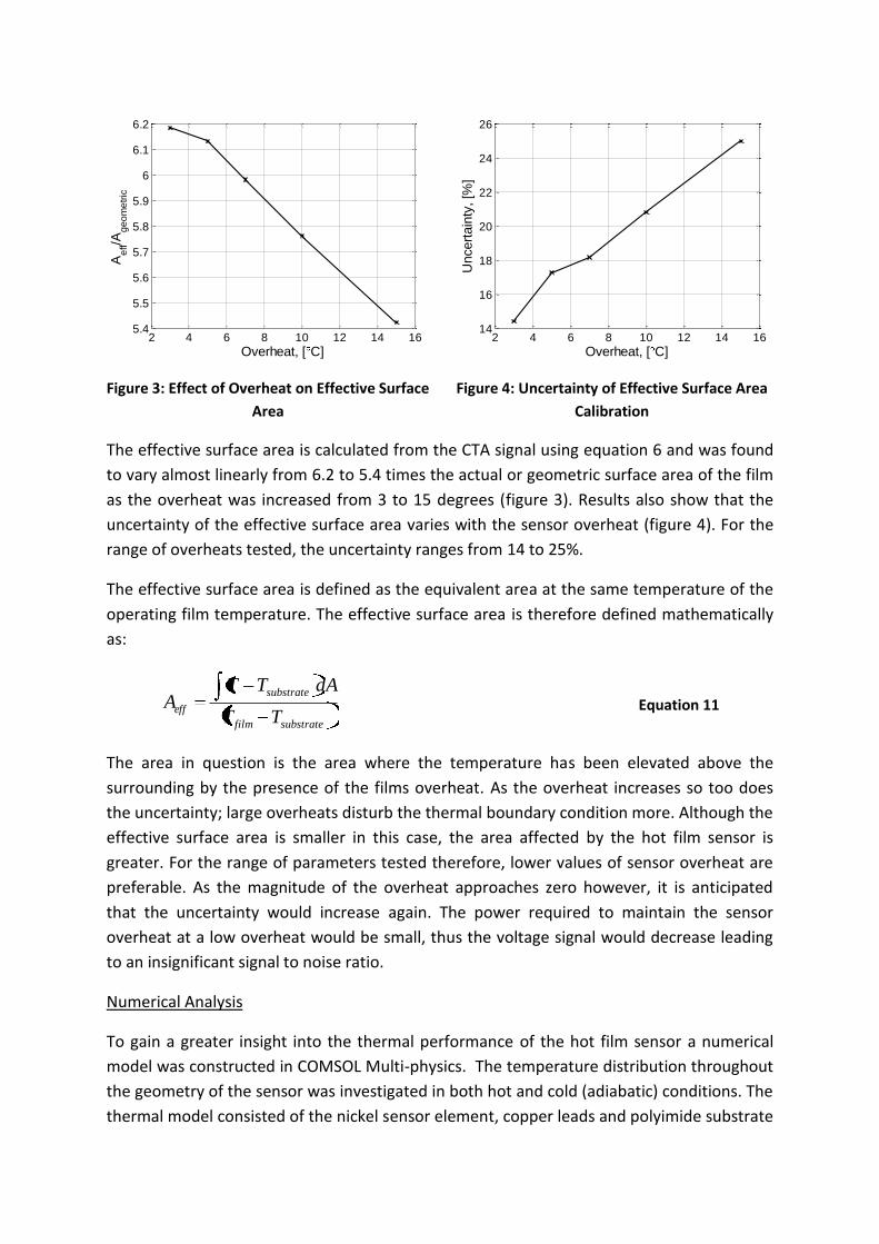
Figure 3: Effect of Overheat on Effective Surface
Area
2 4 6 8 10 12 14 1614
16
18
20
22
24
26
Overheat, [ C]
Uncert
ain
ty, [%
]
Figure 4: Uncertainty of Effective Surface Area
Calibration
The effective surface area is calculated from the CTA signal using equation 6 and was found
to vary almost linearly from 6.2 to 5.4 times the actual or geometric surface area of the film
as the overheat was increased from 3 to 15 degrees (figure 3). Results also show that the
uncertainty of the effective surface area varies with the sensor overheat (figure 4). For the
range of overheats tested, the uncertainty ranges from 14 to 25%.
The effective surface area is defined as the equivalent area at the same temperature of the
operating film temperature. The effective surface area is therefore defined mathematically
as:
substratefilm
substrate
effTT
dATTA
Equation 11
The area in question is the area where the temperature has been elevated above the
surrounding by the presence of the films overheat. As the overheat increases so too does
the uncertainty; large overheats disturb the thermal boundary condition more. Although the
effective surface area is smaller in this case, the area affected by the hot film sensor is
greater. For the range of parameters tested therefore, lower values of sensor overheat are
preferable. As the magnitude of the overheat approaches zero however, it is anticipated
that the uncertainty would increase again. The power required to maintain the sensor
overheat at a low overheat would be small, thus the voltage signal would decrease leading
to an insignificant signal to noise ratio.
Numerical Analysis
To gain a greater insight into the thermal performance of the hot film sensor a numerical
model was constructed in COMSOL Multi-physics. The temperature distribution throughout
the geometry of the sensor was investigated in both hot and cold (adiabatic) conditions. The
thermal model consisted of the nickel sensor element, copper leads and polyimide substrate

as illustrated in figure 5. The dimensions of the sensor were supplied by Senflex and
faithfully modelled in three dimensions. The mesh of the numerical model is illustrated in
figure 6. In excess of 125 thousand prism elements were used in the mesh and it was
concentrated in the regions of highest thermal gradients as indicated.
Figure 5: Model of Sensor Geometry
Figure 6: Numerical Model Mesh
A uniform wall temperature boundary condition was applied beneath the substrate of the
hot film equal to the impingement surface temperature. A uniform convective heat transfer
coefficient determined by the correlation proposed by Shadlesky [22] was applied from the
surface of the hot film sensor element and substrate for each test Reynolds number. The
surface temperature of the Nickel hot film sensor element was set equal to the sum of the
surface temperature and the overheat temperature.
The resulting temperature distribution over the surface of the hot film, where a surface heat
transfer coefficient is 145 W/m2K is presented in figure 7. This is the equivalent stagnation
point heat transfer coefficient reached by a jet (Re = 20,000) where the impingement
surface is placed within the jet core.
Heat from the film, which is at a temperature varying between 3°C and 15°C above that of
the surrounding surface, is conducted to the sensor substrate and copper leads. The
temperature distribution shown in figure 7 indicates that heat from the nickel sensor
element is conducted primarily to the attached copper leads. This has the effect of
increasing the surface area substantially but also non-uniformly. The heated surface area
extends along the copper leads to a distance of more than twice its geometric length, which
reduces the spatial resolution of the technique. Variable heat capacitance and conductivity
of the copper, nickel and polyimide substrate will also influence the response time of the
measurement technique.
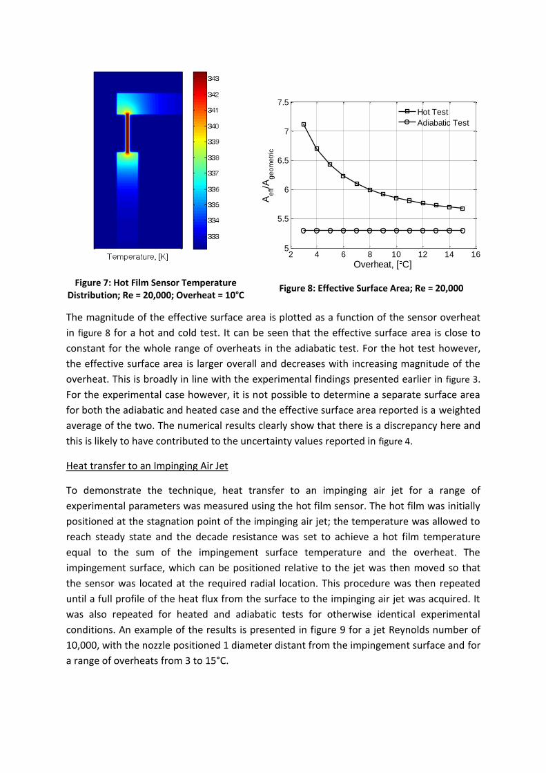
Figure 7: Hot Film Sensor Temperature Distribution; Re = 20,000; Overheat = 10°C
2 4 6 8 10 12 14 165
5.5
6
6.5
7
7.5
Overheat, [ C]A
eff/A
ge
om
etr
ic
Hot Test
Adiabatic Test
Figure 8: Effective Surface Area; Re = 20,000
The magnitude of the effective surface area is plotted as a function of the sensor overheat
in figure 8 for a hot and cold test. It can be seen that the effective surface area is close to
constant for the whole range of overheats in the adiabatic test. For the hot test however,
the effective surface area is larger overall and decreases with increasing magnitude of the
overheat. This is broadly in line with the experimental findings presented earlier in figure 3.
For the experimental case however, it is not possible to determine a separate surface area
for both the adiabatic and heated case and the effective surface area reported is a weighted
average of the two. The numerical results clearly show that there is a discrepancy here and
this is likely to have contributed to the uncertainty values reported in figure 4.
Heat transfer to an Impinging Air Jet
To demonstrate the technique, heat transfer to an impinging air jet for a range of
experimental parameters was measured using the hot film sensor. The hot film was initially
positioned at the stagnation point of the impinging air jet; the temperature was allowed to
reach steady state and the decade resistance was set to achieve a hot film temperature
equal to the sum of the impingement surface temperature and the overheat. The
impingement surface, which can be positioned relative to the jet was then moved so that
the sensor was located at the required radial location. This procedure was then repeated
until a full profile of the heat flux from the surface to the impinging air jet was acquired. It
was also repeated for heated and adiabatic tests for otherwise identical experimental
conditions. An example of the results is presented in figure 9 for a jet Reynolds number of
10,000, with the nozzle positioned 1 diameter distant from the impingement surface and for
a range of overheats from 3 to 15°C.

0 1 2 30
0.5
1
1.5
2
2.5
3x 10
4
r/D
q,
[W/m
2]
0 1 2 30
0.5
1
1.5
2
2.5
3x 10
4
r/D
q,
[W/m
2]
Overheat = 15 C
Overheat = 10 C
Overheat = 7 C
Overheat = 5 C
Overheat = 3 C
(a) Heated Test (b) Adiabatic Test
Figure 9: Distribution of Heat Flux Dissipated to a Jet Impinging at Re=10000, H/D=1.0
Both the heated and adiabatic tests result in similar surface heat flux distributions. The heat
flux is a local minimum at the stagnation point and rises to a peak at a radial location of
approximately 0.75D. It then decreases before rising to a second and third peak at radial
distances of 1.3D and 2.5D approximately. The peaks are less pronounced in the adiabatic
test and the third radial peak is not discernable in most of these profiles. It is also apparent
that the overall magnitude of the surface heat flux is lower for low values of the overheat.
This is due to the small temperature differential between the hot film and the air jet or
impingement surface. While low values of surface heat flux will result in higher values of
measurement uncertainty, higher values result in a higher bias error as the sensor itself can
introduce a significant disturbance in the thermal boundary condition.
To determine the actual surface heat flux by convection to the impinging air jet the
adiabatic value of the surface heat flux is subtracted from the heated test value in
accordance with 9 adiabaticheatedconv qqqairTsurfTT
Equation 9.
The distribution of the Nusselt number has been determined for the data presented in
figure 9 where the temperature differential is the difference between the impingement
surface temperature (Tsurf) and the jet air temperature. These results are presented in figure
10.
0 0.5 1 1.5 2 2.5 320
30
40
50
60
70
r/D
Nu
Overheat = 15 C
Overheat = 10 C
Overheat = 7 C
Overheat = 5 C
Overheat = 3 C
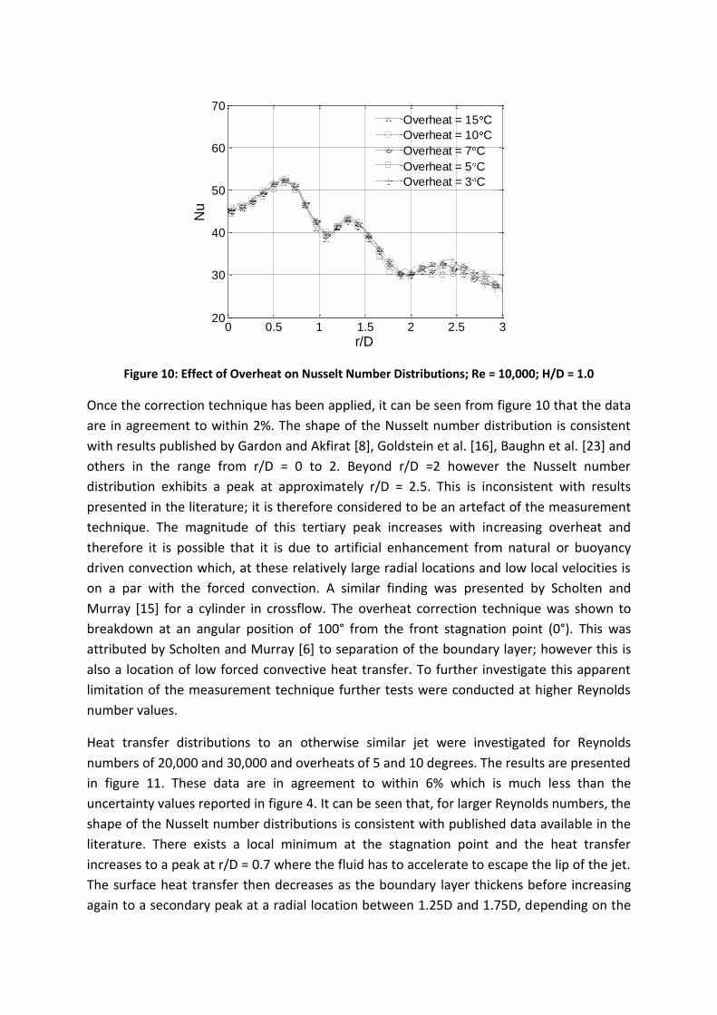
Figure 10: Effect of Overheat on Nusselt Number Distributions; Re = 10,000; H/D = 1.0
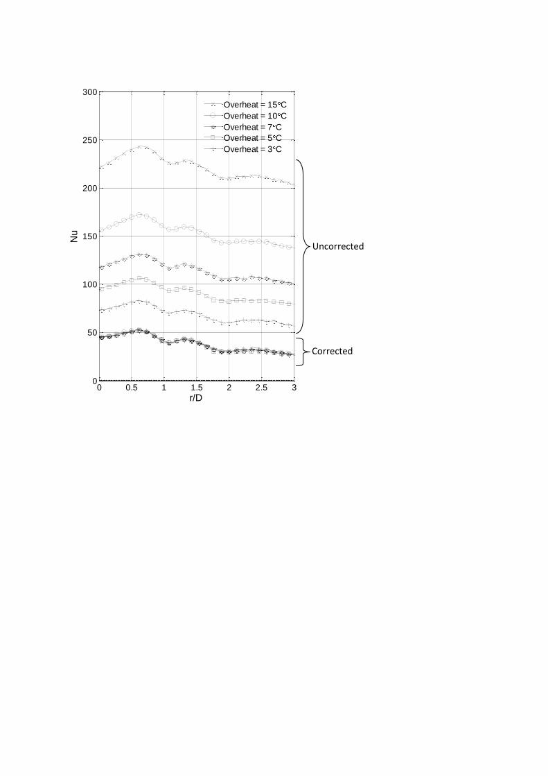
Once the correction technique has been applied, it can be seen from figure 10 that the data
are in agreement to within 2%. The shape of the Nusselt number distribution is consistent
with results published by Gardon and Akfirat [8], Goldstein et al. [16], Baughn et al. [23] and
others in the range from r/D = 0 to 2. Beyond r/D =2 however the Nusselt number
distribution exhibits a peak at approximately r/D = 2.5. This is inconsistent with results
presented in the literature; it is therefore considered to be an artefact of the measurement
technique. The magnitude of this tertiary peak increases with increasing overheat and
therefore it is possible that it is due to artificial enhancement from natural or buoyancy
driven convection which, at these relatively large radial locations and low local velocities is
on a par with the forced convection. A similar finding was presented by Scholten and
Murray [15] for a cylinder in crossflow. The overheat correction technique was shown to
breakdown at an angular position of 100° from the front stagnation point (0°). This was
attributed by Scholten and Murray [6] to separation of the boundary layer; however this is
also a location of low forced convective heat transfer. To further investigate this apparent
limitation of the measurement technique further tests were conducted at higher Reynolds
number values.
Heat transfer distributions to an otherwise similar jet were investigated for Reynolds
numbers of 20,000 and 30,000 and overheats of 5 and 10 degrees. The results are presented
in figure 11. These data are in agreement to within 6% which is much less than the
uncertainty values reported in figure 4. It can be seen that, for larger Reynolds numbers, the
shape of the Nusselt number distributions is consistent with published data available in the
literature. There exists a local minimum at the stagnation point and the heat transfer
increases to a peak at r/D = 0.7 where the fluid has to accelerate to escape the lip of the jet.
The surface heat transfer then decreases as the boundary layer thickens before increasing
again to a secondary peak at a radial location between 1.25D and 1.75D, depending on the
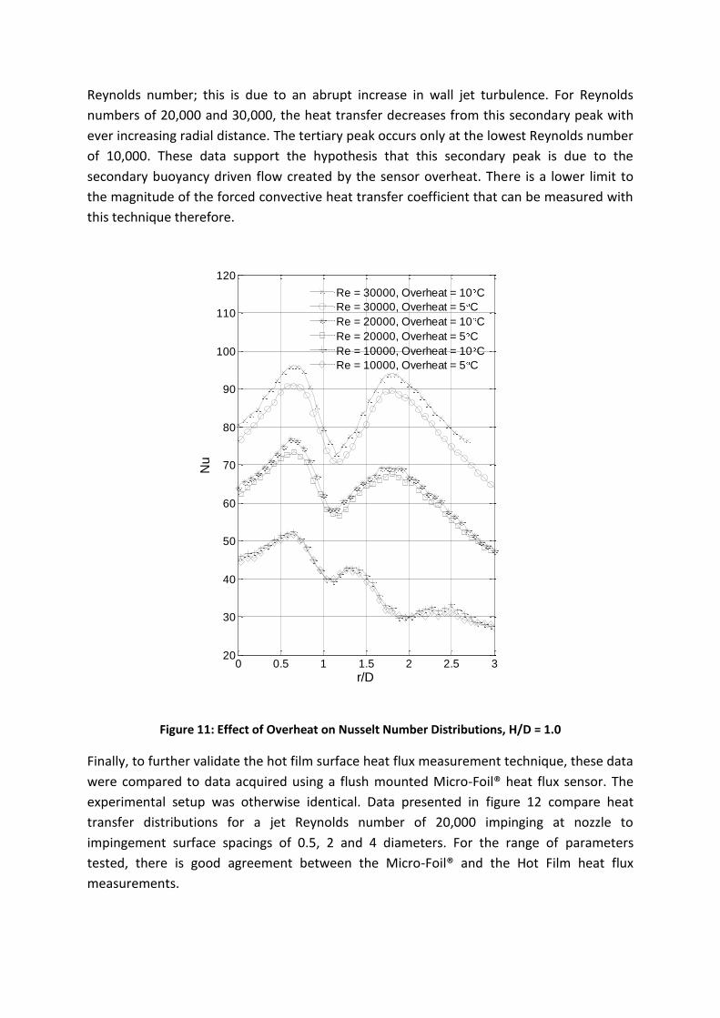
Reynolds number; this is due to an abrupt increase in wall jet turbulence. For Reynolds
numbers of 20,000 and 30,000, the heat transfer decreases from this secondary peak with
ever increasing radial distance. The tertiary peak occurs only at the lowest Reynolds number
of 10,000. These data support the hypothesis that this secondary peak is due to the
secondary buoyancy driven flow created by the sensor overheat. There is a lower limit to
the magnitude of the forced convective heat transfer coefficient that can be measured with
this technique therefore.
0 0.5 1 1.5 2 2.5 320
30
40
50
60
70
80
90
100
110
120
r/D
Nu
Re = 30000, Overheat = 10 C
Re = 30000, Overheat = 5 C
Re = 20000, Overheat = 10 C
Re = 20000, Overheat = 5 C
Re = 10000, Overheat = 10 C
Re = 10000, Overheat = 5 C
Figure 11: Effect of Overheat on Nusselt Number Distributions, H/D = 1.0
Finally, to further validate the hot film surface heat flux measurement technique, these data
were compared to data acquired using a flush mounted Micro-Foil® heat flux sensor. The
experimental setup was otherwise identical. Data presented in figure 12 compare heat
transfer distributions for a jet Reynolds number of 20,000 impinging at nozzle to
impingement surface spacings of 0.5, 2 and 4 diameters. For the range of parameters
tested, there is good agreement between the Micro-Foil® and the Hot Film heat flux
measurements.
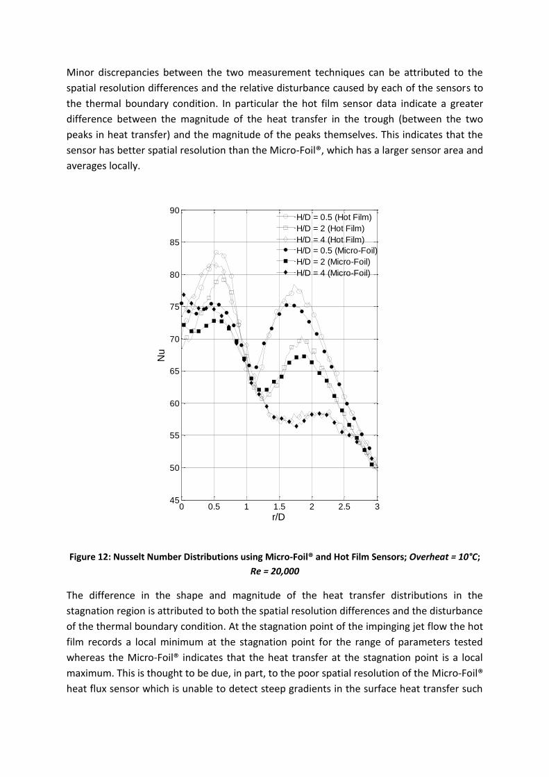
Minor discrepancies between the two measurement techniques can be attributed to the
spatial resolution differences and the relative disturbance caused by each of the sensors to
the thermal boundary condition. In particular the hot film sensor data indicate a greater
difference between the magnitude of the heat transfer in the trough (between the two
peaks in heat transfer) and the magnitude of the peaks themselves. This indicates that the
sensor has better spatial resolution than the Micro-Foil®, which has a larger sensor area and
averages locally.
0 0.5 1 1.5 2 2.5 345
50
55
60
65
70
75
80
85
90
r/D
Nu
H/D = 0.5 (Hot Film)
H/D = 2 (Hot Film)
H/D = 4 (Hot Film)
H/D = 0.5 (Micro-Foil)
H/D = 2 (Micro-Foil)
H/D = 4 (Micro-Foil)
Figure 12: Nusselt Number Distributions using Micro-Foil® and Hot Film Sensors; Overheat = 10°C;
Re = 20,000
The difference in the shape and magnitude of the heat transfer distributions in the
stagnation region is attributed to both the spatial resolution differences and the disturbance
of the thermal boundary condition. At the stagnation point of the impinging jet flow the hot
film records a local minimum at the stagnation point for the range of parameters tested
whereas the Micro-Foil® indicates that the heat transfer at the stagnation point is a local
maximum. This is thought to be due, in part, to the poor spatial resolution of the Micro-Foil®
heat flux sensor which is unable to detect steep gradients in the surface heat transfer such
as occur in the stagnation region. The disturbance of the boundary condition may also be a
factor. Although the hot film sensor operates using a heated element, the thermal mass of
the hot film element is small due to the physical size of the element. The correction
technique also eliminates the bias error created by the presence of the sensor. The Micro-
Foil® however consists of a relatively thick thermal barrier (0.2mm kapton). This contributes
to a significant disturbance of the surface thermal boundary condition that results in
discrepancies with the hot film sensor measurements.
Overall however, the magnitude of the differences between the two techniques is small,
thus validating the new hot film measurement technique for surface heat transfer
measurements.
Conclusions
An improved technique to measure surface heat flux has been presented. A flush mounted
hot film sensor, working in conjunction with a constant temperature anemometer has been
shown to give accurate and repeatable surface heat flux measurements. These results are in
good agreement with previous studies and experimental results achieved using a more
established measurement technique.
It is necessary to maintain the hot film sensor element at a temperature above that of the
surface on which it is mounted. This has been shown to result in a bias error in the surface
heat flux measurement. A technique to correct for this error has been established and
successfully implemented.
A numerical model that demonstrates the thermal performance of the sensor in heated and
adiabatic conditions has also been presented. The magnitude of the effective surface area
calculated is broadly consistent with experimental findings. The magnitude of the effective
surface area has been shown to decrease with increasing magnitude of the overheat. The
connecting copper terminals are primarily responsible for the increased area. Since these
sensors are not designed for this application of surface heat flux measurement and normally
operate at higher overheats to measure wall shear stress, there is scope to improve the
sensor design for heat flux measurement applications.
The magnitude of the overheat has been shown to directly influence the accuracy of the
measurement technique. Larger magnitudes of the overheat disturb the thermal boundary
condition and contribute to the magnitude of the measurement uncertainty. As the
overheat increases, so too does the bias error measured during the adiabatic test. This
amplifies the significance of the difference between the effective surface areas under the
two test conditions. A large overheat also has the potential to cause a significant
disturbance in the thermal boundary condition that will adversely affect the accuracy of the
measurement. This has been demonstrated for instances where the local flow velocity is
low. Careful design of the operating parameters is therefore required to ensure the hot film
technique produces accurate results. As indicated by the numerical model, the magnitude of
the effective surface area is larger when operating under the heated condition than for the
adiabatic condition. It is necessary to assume that this area is constant in practical use to
apply the correction technique. This will also contribute to the uncertainty of the resulting
measurement.
The uncertainty of the measurement technique is shown to decrease as the magnitude of
the overheat tends towards zero. It is expected however, at very low values of the sensor
overheat, that the signal to noise ratio would become insignificant as the power required to
maintain the sensor at very low overheats approaches zero. The limiting value of the sensor
overheat is the subject of future work in this area.
Overall, the hot film technique has been shown to achieve surface heat transfer
measurements that are accurate and with better spatial resolution than other, more
established techniques. While this research has not focused on the temporal response of
the technique the CTA can produce a response in the region of 100 kHz region. It is expected
that some heat capacitance issues may limit this temporal resolution marginally but that it
will remain far in excess of any other surface heat flux measurement technique currently
available. Future work in this area will be develop the technique to measure time-varying
surface heat flux.
References
1. Albrecht, H.-E., N. Damaschke, M. Borys, and C. Tropea, Laser Doppler and phase Doppler measurement techniques. Experimental Fluid Mechanics ed. Springer-Verlag. 2003.
2. Raffel, M., C.E. Willert, S.T. Wereley, and J. Kompenhans, Particle image velocimetry - a practical guide, ed. Springer-Verlag. 2007.
3. Bruun, H.H., Hot-wire anemometry - Principles and signal analysis, ed. O.U. Press. 1995.
4. Jones, P.T.I.a.T.V., The response time of a surface thermometer employing encapsulated thermochromic liquid crystals. Journal of Physics E: Scientific Instruments, 1987. 20(10): p. 1195.
5. Golobic, I., J. Petkovsek, M. Baselj, A. Papez, and D. Kenning, Experimental determination of transient wall temperature distributions close to growing vapor bubbles. Heat and Mass Transfer, 2007.
6. Nakamura, H., Frequency response and spatial resolution of a thin foil for heat transfer measurements using infrared thermography. International Journal of Heat and Mass Transfer, 2009. 52(21-22): p. 5040-5045.
7. Hoogendoorn, C.J., The effect of turbulence on heat transfer at a stagnation point. International Journal of Heat and Mass Transfer, 1977. 20: p. 1333 - 1338.

8. Gardon, R.J. and J.C. Akfirat, The role of turbulence in determining the heat transfer characteristics of impinging jets. International Journal of Heat and Mass Transfer, 1965. 8: p. 1261 - 1272.
9. Liu, T. and J.P. Sullivan, Heat transfer and flow structures in an excited circular impinging jet. International Journal of Heat and Mass Transfer, 1996. 39: p. 3695 - 3706.
10. O'Donovan, T.S. and D.B. Murray, Jet impingement heat transfer - Part I: Mean and root-mean-square heat transfer and velocity distributions. International Journal of Heat and Mass Transfer, 2007. 50(17-18): p. 3291-3301.
11. O'Donovan, T.S. and D.B. Murray, Jet impingement heat transfer - Part II: A temporal investigation of heat transfer and local fluid velocities. International Journal of Heat and Mass Transfer, 2007. 50(17-18): p. 3302-3314.
12. Xie, Q. and D. Wroblewski, Effect of periodic unsteadiness on heat transfer in a turbulent boundary layer downstream of a cylinder-wall junction. International Journal of Heat and Fluid Flow, 1997. 18(1): p. 107-115.
13. Beasley, D.E. and R.S. Figliola, A generalised analysis of a local heat flux probe. Journal of Physics E: Scientific Instrumentation, 1988. 21: p. 316 -322.
14. Moen, M.J. and S.P. Schneider, The effect of sensor size on the performance flush-mounted hot-film sensors. ASME Journal of Fluid Engineering, 1994. 116: p. 273 - 277.
15. Scholten, J.W. and D.B. Murray, Measurement of Convective heat transfer using hot film sensors: Correction for sensor overheat. ASME Journal of Heat Transfer, 1996. 118: p. 982 - 984.
16. Hwang, S.D., C.H. Lee, and H.H. Cho, Heat transfer and flow structures in axisymmetric impinging jet controlled by vortex pairing. International Journal of Heat and Fluid Flow, 2001. 22: p. 293 - 300.
17. Hwang, S.D. and H.H. Cho, Effects of acoustic excitation positions on heat transfer and flow in axisymmetric impinging jet: main jet excitation and shear layer excitation. International Journal of Heat and Fluid Flow, 2003. 24: p. 199 - 209.
18. Smith, B.L. and A. Glezer, The formation and evolution of synthetic jets. Physics of Fluids, 1998. 10: p. 2281 - 2297.
19. Holman, R., Y. Utturkar, R. Mittal, B.L. Smith, and L. Cattafesta, Formation criterion for synthetic jets. AIAA Journal, 2005. 43: p. 2110 - 2116.
20. Persoons, T., A. McGuinn, and D.B. Murray, A general correlation for the stagnation point Nusselt number of an axisymmetric impinging synthetic air jet. International Journal of Heat and Mass Transfer, in review.
21. Goldstein, R.J. and M.E. Franchett, Heat transfer from a flat surface to an oblique impinging jet. ASME Journal of Heat Transfer, 1988. 110: p. 84 - 90.

22. Shadlesky, P.S., Stagnation point heat transfer for jet impingement to a plane surface. AIAA Journal, 1983. 21: p. 1214 - 1215.
23. Baughn, J.W., A.E. Hechanova, and X. Yan, An experimental study of entrainment effects on the heat transfer from a flat surface to a heated circular impinging jet. ASME Journal of Heat Transfer, 1991. 113: p. 1023 - 1025.
0 0.5 1 1.5 2 2.5 30
50
100
150
200
250
300
r/D
Nu
Overheat = 15 C
Overheat = 10 C
Overheat = 7 C
Overheat = 5 C
Overheat = 3 C
Uncorrected
Corrected