hortus modelling horticultural use and supply
TRANSCRIPT

HORTUS Modelling HORTicultural Use and Supply Frank Bunte Michiel van Galen Project code 40150 November 2005 Report 8.05.05 LEI, The Hague

The Agricultural Economics Research Institute (LEI) is active in a wide array of research which can be classified into various domains. This report reflects research within the fol-lowing domain:
Statutory and service tasks Business development and competitive position Natural resources and the environment Land and economics Chains Policy Institutions, people and perceptions Models and data
II

HORTUS; Modelling HORTicultural Use and Supply Bunte, F.H.J. and M.A. van Galen The Hague, LEI, 2005 Report 8.05.05; ISBN 90-8615-032-2; Price € 12.25 (including 6% VAT) 52 pp., fig., tab., app. This report describes the economics and data structure of the HORTUS partial equilibrium supply and demand model developed at LEI. HORTUS can be used to simulate the effects of policy changes and exogenous changes in costs, production and consumer trends on the production, trade and consumption patterns of vegetables and fruits in the Netherlands and other European countries. The report demonstrates the use and working of the model by means of two simulations: (1) a general reduction of import tariffs in the EU and (2) a rise in heating gas prices in the Netherlands. Orders: Phone: 31.70.3358330 Fax: 31.70.3615624 E-mail: [email protected] Information: Phone: 31.70.3358330 Fax: 31.70.3615624 E-mail: [email protected] © LEI, 2005 Reproduction of contents, either whole or in part:
permitted with due reference to the source not permitted
The General Conditions of the Agricultural Research Department apply to all our research commissions. These are registered with the Central Geld-erland Chamber of Commerce in Arnhem.
III

IV
Contents Page Preface 7 Summary 9 1. Introduction 13 2. Supply and demand 15 2.1 Demand 15 2.2 Supply 17 3. Economic structure 22 3.1 Economic structure 22 3.2 Price relations 25 4. Data 28 4.1 Countries, products and inputs 28 4.2 Data sources 29 4.2.1 Supply balances 29 4.2.2 Bilateral trade data 30 4.2.3 Prices 31 4.2.4 Costs 32 4.3 Further data adjustments 32 5. Results 34
5.1 A general reduction in EU import barriers with respect to fruits and 34 Vegetables
5.2 Trade regimes for fruits and vegetables 37 5.3 A rise in Dutch energy costs 41 6. Research agenda 45 References 47 Appendices 1 Definitions of supply balance elements 49 2 Data availability 50 3 Concordance tables for fruits and vegetables 51
5

6
Preface This study outlines HORTUS, an applied partial equilibrium model for European horticul-ture. HORTUS is developed as one of the building stones of the Baseline scenarios developed at LEI. HORTUS enables LEI to make projections of future developments of Dutch and European horticulture. HORTUS may also be used to calculate policy implica-tions of changes in policy variables such as import barriers, energy taxes and so on. Frank Bunte developed the model and constructed the database in co-operation with Michiel van Galen. The study has been guided by Nico de Groot, Andrzej Tabeau and Hans van Meijl. Boudewijn Koole and Marcel Kornelis assisted Frank and Michiel with the data analysis.
Prof. Dr L.C Zachariasse Director General LEI B.V.
7

8
Summary This study makes a first step in developing an applied partial equilibrium model for Euro-pean horticulture: HORTUS. The model outlined in this study is made up of three elements: 1. A set of behavioural equations, more specifically:
- consumer demand for fruits, vegetables and ornamentals; - food industry demand for fruits and vegetables; - producer demand for intermediary inputs, land, labour and capital; - producer supply of fruits, vegetables and ornamentals;
2. A market clearing condition equating demand and supply of fruits, vegetables and ornamentals.
3. A database relating production, trade and consumption of fruits, vegetables and or-namentals. More specifically the database contains: - supply balance sheets, in tonnes, relating production, imports, exports, human
consumption and other uses for every product and region identified (Table 1); - bilateral trade data consistent with aggregate imports and exports from the sup-
ply balance sheets; - producer and export prices. At this stage, only export prices are used in the
model; - cost shares of intermediary inputs, labour and capital and land use for every
product and region identified. Most data are acquired from FAO, WTO/ITC and Eurostat.
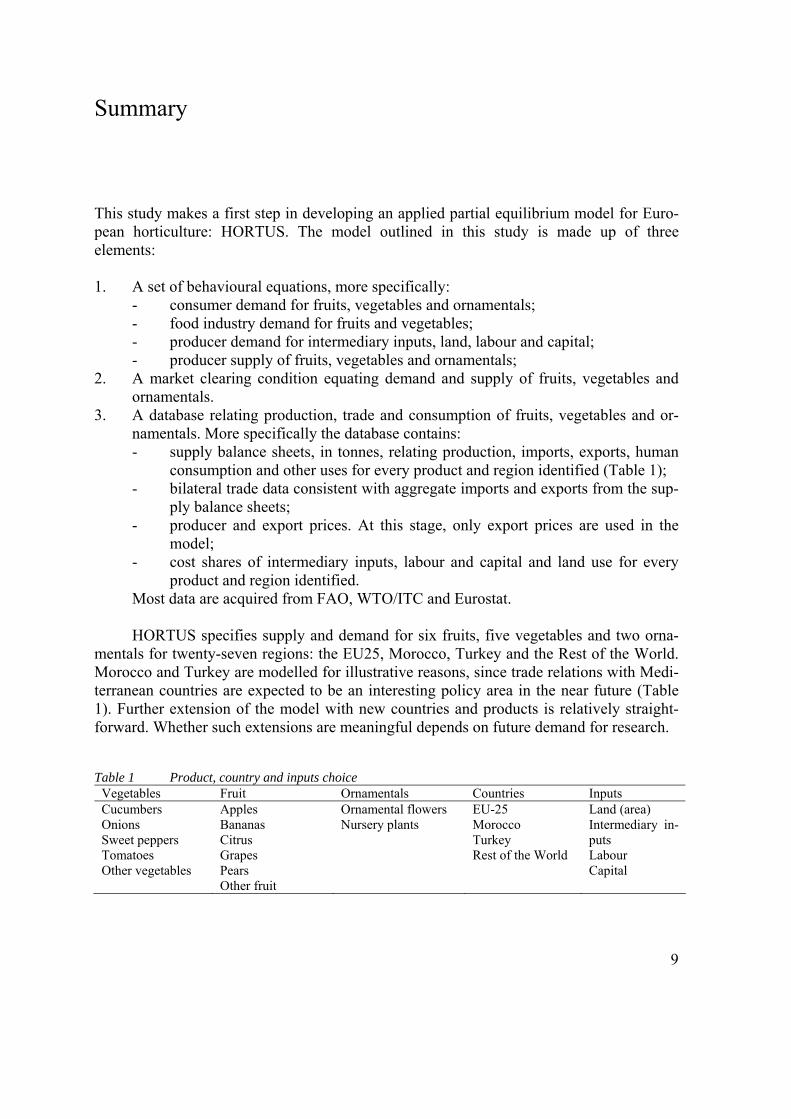
HORTUS specifies supply and demand for six fruits, five vegetables and two orna-
mentals for twenty-seven regions: the EU25, Morocco, Turkey and the Rest of the World. Morocco and Turkey are modelled for illustrative reasons, since trade relations with Medi-terranean countries are expected to be an interesting policy area in the near future (Table 1). Further extension of the model with new countries and products is relatively straight-forward. Whether such extensions are meaningful depends on future demand for research. Table 1 Product, country and inputs choice
Vegetables Fruit Ornamentals Countries Inputs Cucumbers Onions Sweet peppers Tomatoes Other vegetables
Apples Bananas Citrus Grapes Pears Other fruit
Ornamental flowers Nursery plants
EU-25 Morocco Turkey Rest of the World
Land (area) Intermediary in-puts Labour Capital
9
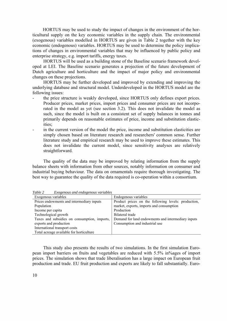
HORTUS may be used to study the impact of changes in the environment of the hor-ticultural supply on the key economic variables in the supply chain. The environmental (exogenous) variables modelled in HORTUS are given in Table 2 together with the key economic (endogenous) variables. HORTUS may be used to determine the policy implica-tions of changes in environmental variables that may be influenced by public policy and enterprise strategy, e.g. import tariffs, energy taxes. HORTUS will be used as a building stone of the Baseline scenario framework devel-oped at LEI. The Baseline scenario generates a projection of the future development of Dutch agriculture and horticulture and the impact of major policy and environmental changes on these projections. HORTUS may be further developed and improved by extending and improving the underlying database and structural model. Underdeveloped in the HORTUS model are the following issues: - the price structure is weakly developed, since HORTUS only defines export prices.
Producer prices, market prices, import prices and consumer prices are not incorpo-rated in the model as yet (see section 3.2). This does not invalidate the model as such, since the model is built on a consistent set of supply balances in tonnes and primarily depends on reasonable estimates of price, income and substitution elastic-ities;
- in the current version of the model the price, income and substitution elasticities are simply chosen based on literature research and researchers' common sense. Further literature study and empirical research may be used to improve these estimates. This does not invalidate the current model, since sensitivity analyses are relatively straightforward.
The quality of the data may be improved by relating information from the supply
balance sheets with information from other sources, notably information on consumer and industrial buying behaviour. The data on ornamentals require thorough investigating. The best way to guarantee the quality of the data required is co-operation within a consortium. Table 2 Exogenous and endogenous variables
Exogenous variables Endogenous variables Prices endowments and intermediary inputs Population Income per capita Technological growth Taxes and subsidies on consumption, imports, exports and production International transport costs Total acreage available for horticulture
Product prices on the following levels: production, market, exports, imports and consumption Production Bilateral trade Demand for land endowments and intermediary inputs Consumption and industrial use
This study also presents the results of two simulations. In the first simulation Euro-pean import barriers on fruits and vegetables are reduced with 5.5% in%ages of import prices. The simulation shows that trade liberalisation has a large impact on European fruit production and trade. EU fruit production and exports are likely to fall substantially. Euro-
10

pean vegetable production and exports are relatively sheltered and are likely to benefit from the decline in EU fruit production. In Europe, horticultural land use will shift from tropical fruits to native fruits and vegetables. Export oriented countries such as Spain (ba-nanas and citrus) and France and the Netherlands (apples) face relatively high adjustment costs in terms of shifts in production. Countries whose production depends on export to Europe (Morocco for citrus and tomatoes) are likely to benefit most. The European land-scape is also likely to benefit. Horticultural production becomes less labour and capital intensive.
The second simulation elaborates on the effects of a rise in energy costs for Dutch glasshouse horticultural producers. The results indicate that a ten% increase in energy prices could cause significant shifts in production and trade flows. In our partial equilib-rium model demand for labour and capital in the effected sectors drops significantly. Due to a substitution effect away from energy intensive crops, glasshouse horticulture would in our short run closure, be more than proportionally affected. Glasshouse vegetables are much more affected than ornamental flowers, because of their energy-intensity. Consump-tion patterns in the Netherlands and Europe are also likely to respond to changing prices.
11

12

1. Introduction For agriculture, several general and partial equilibrium models have been constructed in the post-war period in order to determine the impact of changes in exogenous variables (e.g. agricultural and trade policy) on agricultural production, consumption and trade. For horticulture, however, there are not many economic models relating the production, con-sumption and trade of horticultural products to exogenous variables. There are some partial equilibrium models for specific products, such as bananas. However, there are no eco-nomic models available, which consider the production and trade of horticultural products in Europe and beyond interdependently. There are several reasons why an economic simu-lation model for horticultural products might be a useful addition to the agricultural models available. (1) The economic importance of horticultural production and processing grows, especially in the Netherlands. (2) Horticultural production and trade have a major impact on the environment and consequently are subject to environmental policies, e.g. with re-spect to energy, water and pesticides. Developments in the environment and environmental policies may have major consequences for the division of horticultural production and trade in Europe and beyond. (3) The European Union (EU) is enlarged in 2004 with ten Central and Southern-European countries. Further enlargement and trade liberalisation is foreseen in 2007 and beyond. More in particular, trade liberalisation is foreseen between the EU and the non-EU Mediterranean countries. This might have major consequences for European horticulture, since the Mediterranean is suited for horticultural production, both in Europe, the Middle East and North Africa. In order to gain insight in the quantitative impact of changes in exogenous variables on horticultural production and trade, we need an empirically validated supply and demand model for horticultural products. This report makes a first step in the construction of such a model. We named the first version of our model HORTUS: HORTicultural Use and Sup-ply. This report accounts for the assumptions made in constructing the model. The account refers to four elements: - the supply and demand relations used; - the relation between production, consumption and trade, - the relation between different price levels in the supply chain; and - the data employed.
The report ends with a presentation of preliminary results of simulations made on ba-sis of the model and a research agenda. HORTUS refers to all horticultural products: fruits, vegetables and ornamentals. These three categories are subdivided in more specific product categories, such as apples, tomatoes and cut flowers. Due to data availability, subdivision in more specific product categories is easier for fruits and vegetables than it is for ornamentals. HORTUS refers to all 25 EU-member states and two major non-EU Mediterranean countries: Turkey and Mo-
13
rocco. The latter two are included for illustrative reasons. All other countries are combined in one geographic region: Rest Of the World. The report is constructed as follows. Chapter 2 derives the demand and supply rela-tions employed in the model. Chapter 3 outlines the economic structure: (i) the relation between production, trade, consumption and other uses, and (ii) the relation between the prices in the supply chain. Chapter 4 indicates what data are used and how they are adapted in order to make them fit for the model. Chapter 5 presents some preliminary results. Chapter 6 concludes and presents a research agenda.
14

2. Supply and demand This chapter lays down the demand and supply relations used in HORTUS. The demand and supply relations are derived from utility and production functions. One may guarantee economic consistency by relating demand and supply relations to utility and production functions. At the end of this chapter, we pay attention to matching supply and demand, i.e. market equilibrium. 2.1 Demand The demand for individual commodities is determined using nested CES functions (Figure 2.1). Demand for all commodities within the nest is determined as a function of the nest's budget share and the prices of all commodities with the nest. The prices of all other com-modities only effect demand in as far as they determine the nest's budget share. The aggregate price of fruits determines the budget share of fruits and vegetables. The price of Spanish tomatoes determines the budget share of Spanish versus Dutch tomatoes in Ger-many, but also the aggregate price of imported tomatoes in Germany. The price of Spanish tomatoes effects aggregate tomatoes imports in Germany only indirectly (by influencing the aggregate import price for tomatoes in Germany). There is a fixed budget for fruits and vegetables. Demand substitution between fruits and vegetables on one hand and all other commodities on the other hand will be considered in a later stage. Demand substitution be-tween ornamentals on one hand and all other commodities on the other hand will also considered in a later stage. For the moment, we restrict our attention to the demand for fruits and vegetables on one hand and ornamentals on the other hand. The demand for processed products is neglected for the moment.
Since the demand for product groups and products are determined by CES functions, we derive demand only once. The CES function reads as follows:
⎟⎠⎞⎜
⎝⎛∑=
=yAY i
N
ii
αα
δ1
/1
(2.1)
Y represents the demand for the product group and yi the demand for the individual
commodities, where . A, α and δ∑= yY i i are parameters where .1=∑δ i Parameter α is related to the elasticity of substitution: σ = 1/(1-α). The utility maximisation problem for a nest is defined as follows:
15

VegetablesFruits
Apples Tomatoes
Import Domestic
Budget
Figure 2.1 Demand structure
⎟⎠⎞⎜
⎝⎛ −∑−⎟
⎠⎞⎜
⎝⎛∑=
==IypyAL i
N
iii
N
ii
11
/1
λδ αα
(2.2)
where I indicates the budget and pi commodity i's price. Utility maximisation gives the fol-lowing first order condition.
( ) pyYA iii λδα =−/ 1 (2.3)
Rewriting the first order condition as a function of yi and substituting yi in the budget
constraint, enables one to rewrite λ as a function of income and prices. Substituting λ back into the first order condition enables one to derive commodity demand as a function of in-come and prices:
p σσ
σδ−= 1p
Iyi
ii (2.4)
where represents the price index of Y. Equation (4) may be linearised
by determining the total differential of the equation.
⎟⎠⎞⎜
⎝⎛∑=
=
−−N
ii ip
1
1)1/(1
δ σ σσ
p
16

pp
)( dy
pdpy
dIIy
yd ii
i
iii 1−+−= σσ (2.5)
Dividing by yi simplifies equation (5) to
( )piy ii−+−= pp σ (2.6)
where the 'upper bar' denotes%age changes. Figure 2.2 Supply structure
CES
Leontief
Land
Intermediary input
Labour Capital
Value added
Output
2.2 Supply The production of each commodity j depends on the input of land, labour, capital and in-termediary inputs (Figure 2.2). Following GTAP, we assume a Leontief relation between intermediary inputs on one hand and land, labour and capital on the other hand. The Leon-tief relation allows us to neglect intermediary inputs for the moment: there is simply a linear relation between production and intermediary inputs. The relation between the three production factors and output is modelled using a CES production function. Land is more or less a fixed factor whose input is combined with the input of labour and capital. The CES function employed is the following:
)( M
1iijijjhaj
1/
j xhaγy ∑==
+ ϕϕϕ
γ (2.7)
where yj denotes output of commodity j, haj acreage employed in the production of com-modity j; xij refers to the quantity of input i used in the production of commodity j; and γij and ϕ are parameters. The elasticity of substitution τ is a function of ϕ: τ = 1/(1-ϕ). Acre-age is modelled separately from the other inputs, because total acreage available for
17
agricultural (horticultural) uses is more or less fixed and depends - among other things - on government decisions with respect to rural planning.
A representative producer decides on inputs and outputs using cost minimisation and profit maximisation objectives.
( ) ⎟⎟⎠
⎞⎜⎜⎝
⎛−−−= ∑∑∑∑
== ==
HAhaµxwypxha,ymaxΠM
1jj
M
1j
N
2iiji
M
1jjjijj j
, (2.8)
Producer profits equal revenues: price times quantity (over j commodities) minus
costs: input prices w times input quantities (over all j commodities and all i inputs). Finally profits depend on one physical constraint: the availability of land for horticultural uses. Profits may be maximised using a three step procedure: (1) deciding on non-land inputs by minimising costs; (2) deciding on output by maximising profits; and (3) deciding on acre-age given short run output and price decisions. Input demand The cost minimisation problem is modelled as follows:
( ) ⎟⎟⎠
⎞⎜⎜⎝
⎛⎟⎟⎠
⎞⎜⎜⎝
⎛−∑−= ∑ +∑∑
= == =
M
1jj
N
2iijijjhaj
1/M
1j
N
2iijiij yxhaγλxwxCmin )( ϕϕ
ϕ
γ (2.9)
where C represents non-land production costs. The first order condition of the optimisation problem equals:
( )xyγλw ijj
1
iji / ϕ−= (2.10)
Rewriting the first order condition as a function of xij and substituting xij in the pro-
duction function gives an expression for λ. Substituting λ back into the first order condition gives:
⎟⎠⎞
⎜⎝⎛
⎟⎠⎞
⎜⎝⎛
−=AP
MP1
w
γyx
j
j
1
i
ij
τ
jij
ϕ/
jw (2.11)
where represents the aggregate input price for commodity j. ( )wγ iτ1N
2iij
τ τ)1/(1−
=
−
∑=wj
The demand for input i for the production of commodity j depends on the production of commodity j (yj), the price of input i (wi) versus the aggregate input price (wj) and the
returns to non-land factor inputs ⎟⎠
⎞⎜⎝
⎛=
y
haγ
APMP
j
j
hajhaj
haj
ϕ
, where MPhaj denotes the marginal
18

product of land for commodity j and APhaj the average product of land for commodity j, i.e. the yield for commodity j.
In a linearised form the demand for factor inputs transforms to:
ydyx
APMP-1APMP
hadhax
APMP-1APMP
wdwxτdxτyd
yx
xd jj
ij
hajhaj
hajhajj
j
ij
hajhaj
hajhaji
i
ijijj
j
ijij ⎟⎟
⎠
⎞⎜⎜⎝
⎛+⎟⎟
⎠
⎞⎜⎜⎝
⎛−−+= w
wj
j
or
( ) ( hayπwτyx jjjijij −+−+= wj ) . (2.12)
where ⎟⎟⎠
⎞⎜⎜⎝
⎛
−=
APMP1APMP
πhajhaj
hajhajj . The last term on the right hand side models diminishing re-
turns to labour and capital.1 If output is to increase more than acreage input ( )hay jj > ,
labour and capital input should increase with a factor ( )( )hayπ jjj − above the output in-
crease ( )yj . Supply One may derive short-run output yj (or equivalently short-run price pj) as a function of equilibrium inputs xij by substituting xij into the profit function (equation (2.9)) and maxi-mising this function towards yj.
( ) ∑∑∑= ==
−=M
1j
N
2iiji
M
1jjjj xwypymaxΠ (2.13)
The first order derivative equals
⇔=∂∂
−=∂∂ ∑
=
0yx
wpy j
ijN
2iij
j
Π
⎥⎦⎤
⎢⎣⎡ −=
AP
MP1p
haj
haj
1
j
ϕ/
jw (2.14)
using equation (2.12). The supply price pj depends on aggregate input costs wj and dimin-ishing returns to capital and labour input given acreage. Linearising this function gives the short-run inverse supply function: 1 Note that πj is only positive when returns are in fact increasing: MPj < APj. Note also that πj is endogenous, since it depends on yj and haj.
19

( )hayπp jjjj −+= wj (2.15) Acreage The last optimisation problem refers to acreage input: how does the producer divide avail-able acreage over the respective commodities to be produced. This problem is solved by maximising the profit maximisation problem:
( ) ⎟⎟⎠
⎞⎜⎜⎝
⎛−−−= ∑∑∑∑
== ==
HAhaµxwyphamaxΠM
1jj
M
1j
N
2iiji
M
1jjjj (2.16)
The first order condition is as follows:
( )⎟⎟⎠
⎞⎜⎜⎝
⎛−−
∂∂
∂∂−
∂
∂=
∂∂
∑∑∑∑== ==
HAhaµhax
xxw
ha
yp
hahaΠ M
1jj
M
1j
N
2i j
ij
ij
ijiM
1j j
j j
j
j (2.17)
Since ∂wixij/∂xij = 0 due to the first order condition in the cost minimisation problem, this expression reduces to
( )⎟⎟⎠
⎞⎜⎜⎝
⎛−−
∂
∂=
∂∂
∑∑==
HAhaµha
yp
hahaΠ M
1jj
M
1j j
j j
j
j (2.18)
The first order condition thus equals:
( ) µhayγp jj
1
hajj / =−ϕ
(2.19) Rewriting the first order condition as a function of haj and substituting haj in the produc-tion function gives an expression for µ. Substituting µ back into the first order condition gives:
( )( )( )( )∑
=
=
−
M
1jjhaj
-1/(1j
jhaj
11
jj
pγy
pyHAha
)
)/(
ϕ
ϕγ
(2.20)
One may linearise this equation to the following equation:
∑∑−
≠
−
≠⎟⎟⎠
⎞⎜⎜⎝
⎛−⎟⎟
⎠
⎞⎜⎜⎝
⎛−⎥
⎦
⎤⎢⎣
⎡+⎥
⎦
⎤⎢⎣
⎡+=
1M
jkk
k
kj
1M
jkk
k
kjj
j
j
jj
j
j
jjj pd
pHAhaτhayd
yHAhahapd
HAha-1
phayd
HAha-1
yhadHA
HAha
had τ
20
or
[ ] [ ] ( ) ( )∑∑−
≠
−
≠
−−++=1M
jkkk
1M
jkkkjjjjj pτsysps-1ys-1HAha τ (2.21)
where sj = haj/HA denotes the share of the land used for commodity j divided by all land available. Acreage available for commodity j depends positively on total acreage (HA) and the output and price of commodity j (yj and pj respectively) and the output and price of all other commodities k (yk and pk respectively).
21
3. Economic structure This chapter presents the economic used in structure in HORTUS. Section 3.1 relates pro-duction and international trade to consumption and other uses. The economic structure is explained in terms of commodity balances, supply and use and ultimately input-output ta-bles. Although the HORTUS model does not yet employ a full scale input-output structure it is nevertheless a useful way to discuss the economic relations in a multi-sector, multi-country model. Section 3.2 relates prices at the various stages of the supply chain to each other. The price relations make it possible to model changes in taxes and subsidies, and discern between prices at e.g. a consumer level and producer level. 3.1 Economic structure The economic structure in HORTUS is based on commodity balances. Commodity bal-ances are the most simple economic framework relating supply and use of a certain product in a certain country. Supply S in region r equals the sum of domestic production P and im-ports M.1 Domestic use U equals the difference of supply S and exports X.2 Domestic use U may be subdivided in human consumption C, processing I and other uses O (feed, seed, industrial use and other uses not else specified). In an equation: P+M = S = X+U = X+C+I+O. (3.1) Table 3.1 below shows commodity balances for tomatoes, for the EU-15 countries minus Luxemburg. HORTUS identifies quantities on the one hand and values and prices on the other hand. Note that the commodity balances are constructed on basis of quantities. In-formation on prices is added in a later stage to arrive at an economic structure in terms of monetary values.
1 Full scale supply tables relate the domestic supply of each product to each industry, recognizing the fact that some industries might produce more than one product and some products are produced by more than one industry. 2 A full scale use table indicates the use of all goods and services by product and type of use: intermediate consumption by industry, final consumption by consumers and government, gross capital formation and ex-ports. The use table also presents the elements of value added by industry.
22

Tabl
e 3.
1 C
omm
odity
bal
ance
s for
fres
h to
mat
oes (
in to
nnes
)
Prod
uctio
n Im
ports
Su
pply
Ex
port
Dom
estic
use
C
onsu
mpt
ion
Proc
essi
ng
Oth
er u
ses
Con
sum
ptio
n pe
r cap
ita
Bel
gium
31
5,50
3 49
,450
36
4,95
3 17
4,97
5 18
9,97
8 16
1,97
3 7,
847
20,1
58
15.3
D
enm
ark
21,2
38
109,
971
131,
209
11,7
16
119,
493
119,
943
0 0
22.6
G
erm
any
37,0
00
649,
000
686,
000
12,0
00
674,
000
607,
000
0 67
,000
7.
4 G
reec
e 1,
899,
100
6,33
0 1,
905,
430
7,50
0 1,
897,
930
677,
630
1,22
0,30
0 0
64.5
Sp
ain
3,51
0,70
0 7,
400
3,51
8,10
0 89
5,90
0 2,
622,
200
597,
900
1,39
0,00
0 63
4,30
0 15
.2
Fran
ce
899,
000
383,
000
1,28
2,00
0 91
,000
1,
191,
000
774,
000
328,
000
89,0
00
13.2
Ir
elan
d 7,
000
15,0
00
22,0
00
1,00
0 21
,000
20
,000
0
1,00
0 5.
4 Ita
ly
5,97
7,00
0 38
,000
6,
013,
000
126,
000
5,88
9,00
0 1,
525,
000
4,35
2,00
0 12
,000
26
.5
Net
herla
nds
510,
000
168,
000
678,
000
636,
000
42,0
00
42,0
00
0 0
2.7
Aus
tria
16,9
00
49,1
00
66,0
00
2,10
0 63
,900
57
,300
0
6,60
0 7.
1 Po
rtuga
l 1,
130,
000
15,0
00
1,14
5,00
0 4,
000
1,14
1,00
0 67
,000
98
8,00
0 86
,000
6.
7 Fi
nlan
d 31
,500
28
,600
60
,100
30
0 59
,800
59
,800
0
0 12
.0
Swed
en
23,9
00
65,1
00
89,0
00
700
88,3
00
69,4
00
0 18
,900
7.
9 U
K
119,
300
287,
000
406,
300
4,00
0 40
2,30
0 40
0,30
0 0
2,00
0 6.
8 So
urce
: Eur
osta
t (20
00).
23
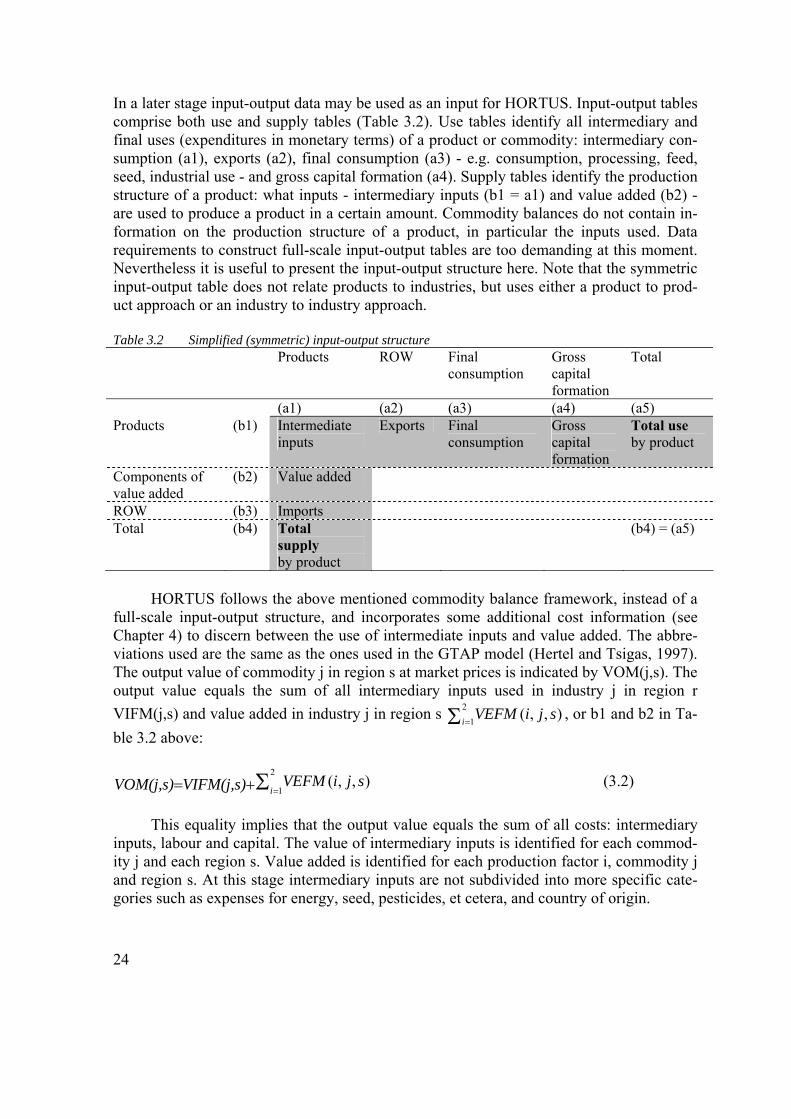
In a later stage input-output data may be used as an input for HORTUS. Input-output tables comprise both use and supply tables (Table 3.2). Use tables identify all intermediary and final uses (expenditures in monetary terms) of a product or commodity: intermediary con-sumption (a1), exports (a2), final consumption (a3) - e.g. consumption, processing, feed, seed, industrial use - and gross capital formation (a4). Supply tables identify the production structure of a product: what inputs - intermediary inputs (b1 = a1) and value added (b2) - are used to produce a product in a certain amount. Commodity balances do not contain in-formation on the production structure of a product, in particular the inputs used. Data requirements to construct full-scale input-output tables are too demanding at this moment. Nevertheless it is useful to present the input-output structure here. Note that the symmetric input-output table does not relate products to industries, but uses either a product to prod-uct approach or an industry to industry approach. Table 3.2 Simplified (symmetric) input-output structure Products ROW Final
consumption Gross capital formation
Total
(a1) (a2) (a3) (a4) (a5) Products (b1) Intermediate
inputs Exports Final
consumption Gross capital formation
Total use by product
Components of value added
(b2) Value added
ROW (b3) Imports Total (b4) Total
supply by product
(b4) = (a5)
HORTUS follows the above mentioned commodity balance framework, instead of a
full-scale input-output structure, and incorporates some additional cost information (see Chapter 4) to discern between the use of intermediate inputs and value added. The abbre-viations used are the same as the ones used in the GTAP model (Hertel and Tsigas, 1997). The output value of commodity j in region s at market prices is indicated by VOM(j,s). The output value equals the sum of all intermediary inputs used in industry j in region r VIFM(j,s) and value added in industry j in region s ),,(2
1 sjiVEFMiΣ =, or b1 and b2 in Ta-
ble 3.2 above:
),,(2
1sjiVEFMVIFM(j,s)VOM(j,s) iΣ+= =
(3.2)
This equality implies that the output value equals the sum of all costs: intermediary inputs, labour and capital. The value of intermediary inputs is identified for each commod-ity j and each region s. Value added is identified for each production factor i, commodity j and region s. At this stage intermediary inputs are not subdivided into more specific cate-gories such as expenses for energy, seed, pesticides, et cetera, and country of origin.
24

The available amount, or total supply of commodities in a country VOIM(j,s) equals the sum of production and imports.
),,( srjVIMSVOM(j,s)VOIM(j,s)R
rΣ+= =1 (3.3)
Import value VIM(j,r,s) is identified for each commodity j, country of origin r and country of destination s. There are two possible destinations for the supply available: do-mestic use and exports. Domestic use is subdivided into human consumption, processing and other uses. There is no subdivision into private and public purchases (consumers and firms versus government). Available supply in region s may thus be subdivided into:
),,(1
srjVXMDVPM(j,s)VOIM(j,s)R
sΣ+= = (3.4)
Private consumption is identified for each commodity j and region s. Exports are
identified for each commodity j, country of origin r and country of destination s. Private consumption is subdivided into two categories: domestic origin (VDPM) and imports (VIPM) VPM(j,s) = VDPM(j,s)+VIPM(j,s). (3.5) Consumption is identified for each commodity j and region s. Imports are aggregated for this purpose. 3.2 Price relations HORTUS identifies a great number of prices: producer prices, market prices, export prices, import prices and consumer prices. Figure 3.1 relates the prices identified in HORTUS. The prices differ from each other due to taxes, subsidies, import and export taxes and sub-sidies, trade margins and transport costs. In this section, we follow the product from producer to consumer and distinguish all relevant price levels (Figure 3.1). The producer receives producer price PS. If the product is taxed or subsidised, output tax TO creates a wedge between the producer price PS and the market price PM. The commodity is sold for domestic use or exports. Consumer tax and trade margins TPD cre-ate a wedge between the market price PM and the consumer price PPD. Commodities are exported at export price Pfob. The difference between the market price PM and the export price Pfob is equal to the export tax TXS. Import prices Pcif are obtained by adding transport costs Tcost to the free on board export prices Pfob. The market price of imported commodi-ties PMS may be obtained by adding import taxes TMS to the import price Pcif. Again, for imported products consumer taxes TPM create a wedge between market prices PM and consumer prices PPM. The model also identifies the input prices the producers face as well as the taxes and subsidies on these inputs. These taxes may be used to model e.g. changes in energy policy.
25
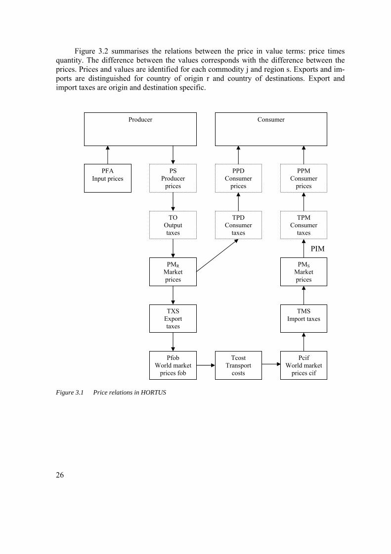
Figure 3.2 summarises the relations between the price in value terms: price times quantity. The difference between the values corresponds with the difference between the prices. Prices and values are identified for each commodity j and region s. Exports and im-ports are distinguished for country of origin r and country of destinations. Export and import taxes are origin and destination specific.
PIM
PFA Input prices
PS Producer
prices
Producer
TO Output taxes
PMR Market prices
TXS Export taxes
PMS Market prices
TPM Consumer
taxes
TPD Consumer
taxes
PPD Consumer
prices
PPM Consumer
prices
Consumer
TMS Import taxes
Tcost Transport
costs
Pcif World market
prices cif
Pfob World market
prices fob
Figure 3.1 Price relations in HORTUS
26

VDPM
VXMD
VIM
VFA VOA
Producer
PTAX
VOM
XTAXD
VT VIWS
MTAX
VIMS
IPTAX DPTAX
VDPA
VIPA
Consumer
VXWD
Figure 3.2 Relation between production, trade and consumption values in HORTUS
27
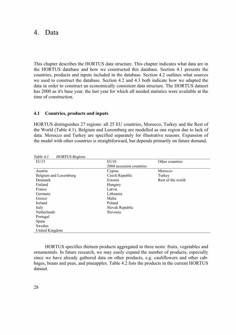
4. Data This chapter describes the HORTUS data structure. This chapter indicates what data are in the HORTUS database and how we constructed this database. Section 4.1 presents the countries, products and inputs included in the database. Section 4.2 outlines what sources we used to construct the database. Section 4.2 and 4.3 both indicate how we adapted the data in order to construct an economically consistent data structure. The HORTUS dataset has 2000 as it's base year, the last year for which all needed statistics were available at the time of construction. 4.1 Countries, products and inputs HORTUS distinguishes 27 regions: all 25 EU countries, Morocco, Turkey and the Rest of the World (Table 4.1). Belgium and Luxemburg are modelled as one region due to lack of data. Morocco and Turkey are specified separately for illustrative reasons. Expansion of the model with other countries is straightforward, but depends primarily on future demand. Table 4.1 HORTUS Regions
EU15 EU10 2004 accession countries
Other countries
Austria Cyprus Morocco Belgium and Luxemburg Czech Republic Turkey Denmark Estonia Rest of the world Finland Hungary France Latvia Germany Lithuania Greece Malta Ireland Poland Italy Slovak Republic Netherlands Slovenia Portugal Spain Sweden United Kingdom
HORTUS specifies thirteen products aggregated in three nests: fruits, vegetables and ornamentals. In future research, we may easily expand the number of products, especially since we have already gathered data on other products, e.g. cauliflowers and other cab-bages, beans and peas, and pineapples. Table 4.2 lists the products in the current HORTUS dataset.
28
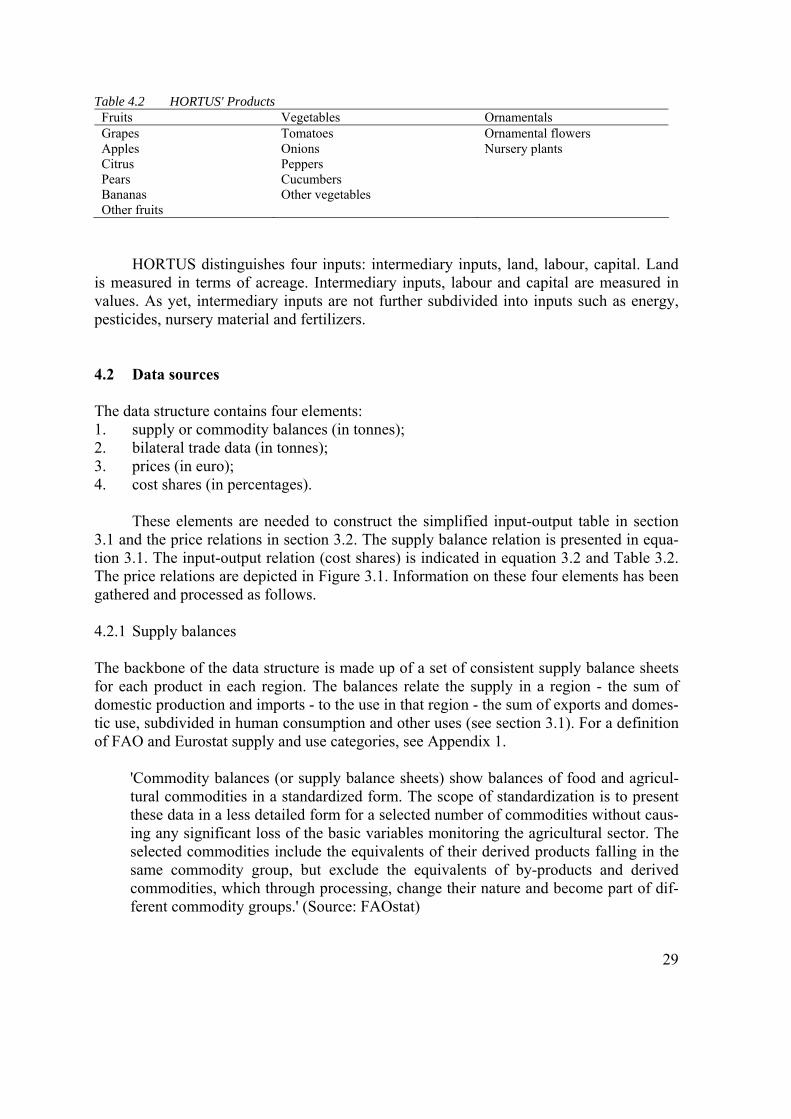
Table 4.2 HORTUS' Products Fruits Vegetables Ornamentals Grapes Tomatoes Ornamental flowers Apples Onions Nursery plants Citrus Peppers Pears Cucumbers Bananas Other vegetables Other fruits
HORTUS distinguishes four inputs: intermediary inputs, land, labour, capital. Land is measured in terms of acreage. Intermediary inputs, labour and capital are measured in values. As yet, intermediary inputs are not further subdivided into inputs such as energy, pesticides, nursery material and fertilizers. 4.2 Data sources The data structure contains four elements: 1. supply or commodity balances (in tonnes); 2. bilateral trade data (in tonnes); 3. prices (in euro); 4. cost shares (in percentages).
These elements are needed to construct the simplified input-output table in section 3.1 and the price relations in section 3.2. The supply balance relation is presented in equa-tion 3.1. The input-output relation (cost shares) is indicated in equation 3.2 and Table 3.2. The price relations are depicted in Figure 3.1. Information on these four elements has been gathered and processed as follows. 4.2.1 Supply balances The backbone of the data structure is made up of a set of consistent supply balance sheets for each product in each region. The balances relate the supply in a region - the sum of domestic production and imports - to the use in that region - the sum of exports and domes-tic use, subdivided in human consumption and other uses (see section 3.1). For a definition of FAO and Eurostat supply and use categories, see Appendix 1.
'Commodity balances (or supply balance sheets) show balances of food and agricul-tural commodities in a standardized form. The scope of standardization is to present these data in a less detailed form for a selected number of commodities without caus-ing any significant loss of the basic variables monitoring the agricultural sector. The selected commodities include the equivalents of their derived products falling in the same commodity group, but exclude the equivalents of by-products and derived commodities, which through processing, change their nature and become part of dif-ferent commodity groups.' (Source: FAOstat)
29
We derive commodity balances from two main sources: FAOstat Supply Balance Sheets and Eurostat Agris Table. These sources contain more or less complete commodity balances for most products and countries. For other products - notably cucumbers, peppers and ornamentals - and countries, commodity balances have been constructed on basis of production and trade data (Appendix 2). For this purpose, FAOstat and ITC/WTO produc-tion and trade data have been used. For these cases, we assume that all domestic use equals human consumption. In general, if we do not have data on other uses, we assume that all domestic use equals human consumption. Appendix 2 gives an overview of the sources per product and per region.
HORTUS distinguishes two categories of domestic use: human consumption and other uses. Besides other uses such as industrial uses, seed and feed, the FAO and Eurostat supply balances distinguish losses and stock changes. Whenever other uses are positive, the data on losses and stock changes in the original data are reflected in other uses in the HORTUS dataset. If not, the data on losses and stock changes in the original data are re-flected in human consumption in the HORTUS dataset.
We construct commodity balances for Other Fruits and Other Vegetables by adding up data for a number of individual products and product categories. Production and land area data, as well as aggregate imports and exports are taken from Faostat. Products in-cluded in the two categories are listed in Appendix 3. Bilateral trade data for Other Fruits and Other Vegetables include all fresh or chilled produce from ITC/WTO data not in-cluded in one of the other categories in the model. Producer prices of other vegetables and fruits are computed from Faostat local currency data, using average euro exchange rates for 2000 for the HORTUS countries.
There are little data for ornamentals. We distinguish two groups of ornamentals from the Eurostat Agris tables: Ornamental flowers and plants, and Nursery material. Supply balances are constructed on basis of production values rather than volumes as the former are more accurate and consistent. Ornamentals' prices are set equal to one, their numéraire value. To complete the supply balance sheets import and export values are added from the ITC/WTO bilateral trade database. Production in the Rest of the World is estimated on ba-sis of AIPH data. 4.2.2 Bilateral trade data Bilateral trade data have been collected for each product, each country of origin and each country of destination. The most important data source used for constructing the dataset on bilateral trade is the PCTAS database (ITC/WTO). PCTAS does not disaggregate products to the same levels as Comext does, but contains data on more countries than Comext does. Comext is only made up of EU countries. Only for peppers, one has to resort to Comext data. Bilateral trade relations involving the Rest of the World have been imputed from ag-gregate exports and imports and bilateral exports and imports of all other regions (Table 4.3).
30
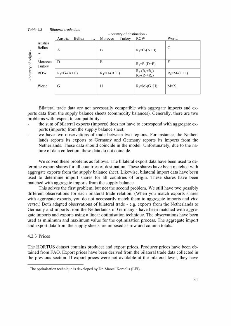
Table 4.3 Bilateral trade data - country of destination -
Austria Bellux … Morocco Turkey ROW World Austria Bellux … …
A B R1=C-(A+B) C
Morocco Turkey
D
E R2=F-(D+E) F
ROW R3=G-(A+D) R4=H-(B+E) R5-(R1+R2) R6-(R3+R4)
R6=M-(C+F)
- cou
ntry
of o
rigin
-
World G
H
R5=M-(G+H) M=X
Bilateral trade data are not necessarily compatible with aggregate imports and ex-ports data from the supply balance sheets (commodity balances). Generally, there are two problems with respect to compatibility: - the sum of bilateral exports (imports) does not have to correspond with aggregate ex-
ports (imports) from the supply balance sheet; - we have two observations of trade between two regions. For instance, the Nether-
lands reports its exports to Germany and Germany reports its imports from the Netherlands. These data should coincide in the model. Unfortunately, due to the na-ture of data collection, these data do not coincide.
We solved these problems as follows. The bilateral export data have been used to de-
termine export shares for all countries of destination. These shares have been matched with aggregate exports from the supply balance sheet. Likewise, bilateral import data have been used to determine import shares for all countries of origin. These shares have been matched with aggregate imports from the supply balance This solves the first problem, but not the second problem. We still have two possibly different observations for each bilateral trade relation. (When you match exports shares with aggregate exports, you do not necessarily match them to aggregate imports and vice versa.) Both adapted observations of bilateral trade - e.g. exports from the Netherlands to Germany and imports from the Netherlands in Germany - have been matched with aggre-gate imports and exports using a linear optimisation technique. The observations have been used as minimum and maximum value for the optimisation process. The aggregate import and export data from the supply sheets are imposed as row and column totals.1 4.2.3 Prices The HORTUS dataset contains producer and export prices. Producer prices have been ob-tained from FAO. Export prices have been derived from the bilateral trade data collected in the previous section. If export prices were not available at the bilateral level, they have 1 The optimisation technique is developed by Dr. Marcel Kornelis (LEI).
31

been substituted with export prices at the aggregate level. Ornamentals' export prices equal their numéraire value, i.e we set prices equal to 1 euro per kilogram for the moment.
At this moment, HORTUS calculates all values in the model using export prices. Producer prices are not used, as yet. At this moment, we compare export and producer prices before incorporating the latter into the model. 4.2.4 Costs To relate horticultural output to its inputs we make use of the RICA database. This Euro-stat database contains figures on production costs and value added for a selection of vegetables and fruits. These data are available for citrus fruit, grapes, tomatoes, leafy and stem vegetables, other vegetables, pomes, and tropical fruit. Each of the products identified in the model is put in one of the abovementioned categories. For some countries, notably small countries and the regions outside the EU, we used data on other countries. For small European countries we used data on neighbour countries (see Bunte 2000). For the non-EU regions, we used the average of a number of southern European countries.
From the RICA database we extract the following information: - turnover; - intermediary costs of production; - expenses on labour and capital; - opportunity costs of unpaid-labour and capital.
Expenses on intermediary inputs and paid labour and capital refer to actually in-curred costs. The cost shares of these inputs are simply determined as their share in total turnover. For unpaid labour and capital, we determined their opportunity costs. These op-portunity costs are matched proportionally to the difference between turnover and actual expenses on intermediary inputs and paid labour and capital. 4.3 Further data adjustments The economic model specifies the country of origin for all products consumed. Germans consume X tonnes of domestic tomatoes, Y tonnes of Dutch tomatoes, Z tonnes of Spanish tomatoes and A tonnes of other tomatoes. Theoretically, we do not have a problem with this fact. In practice, re-exports complicate the picture. How Dutch are Dutch tomatoes? Countries may export products that they do not produce, e.g. bananas exported by Bel-gium. Countries may export more than they produce, e.g. Dutch tomatoes. Re-export poses a theoretical and an empirical challenge. The theoretical problem refers to the fact that if one allows both production and re-export in the model, one introduces two sources for ex-ports in the model: producing countries and re-exporting countries. The import and exports variables would need 4 dimensions (section 3.1). The empirical problem refers to the dis-tinction to be made in the data: what is export and what is re-export, and how are both variables linked. In order to keep things simple, we do not allow re-exports in the model. We source trade flows back to the producing country. This is appropriate, since we are primarily interested in the question how changes in international trade influence changes in
32

horticultural production. In order to rule out re-exports, we have applied the following ad-justments: 1. No production, but positive exports (e.g. bananas from Belgium)
Countries that do not produce a certain product, do not export it. This holds primarily for tropical fruits: bananas, citrus and to some extent grapes. For these countries, we as-sume the following. Exports are zero, imports equal net imports leaving production (zero), human consumption and other uses unchanged. Bananas are produced in seven regions: Spain, Portugal, Greece, Cyprus, Morocco, Turkey and the Rest of the World. Citrus is produced in these seven countries plus France, Malta and Italy. Grapes are produced in all countries, except for Scandinavia, the Baltic States, Ireland and Poland. Chillies and peppers are produced in the grapes producing countries with the exception of Germany.
2. Positive production, but exports exceed production (e.g. tomatoes in the Netherlands)
In a limited number of cases, a region exports more than it produces. This holds prima-rily for Belgium-Luxemburg and the Netherlands. In these cases, exports and imports have been adjusted downwards in the same amounts, leaving domestic use (and pro-duction) unaffected.
33

5. Results In this section, we present the results of two simulations performed with HORTUS: (1) a general reduction in EU import barriers with respect to fruits and vegetables; and (2) an in-crease in gas prices in the Netherlands, for instance due to unilateral Dutch climate policy. The first simulation is discussed in section 5.1 and 5.2 and the second simulation in section 5.3. 5.1 A general reduction in EU import barriers with respect to fruits and vegetables Table 5.1 presents some key data on the EU fruits and vegetables supply for the former EU15. Two thirds of the EU's fruits and vegetables consumption is produced domestically (excluding intra-European trade). So, one third of the EU's fruits and vegetables consump-tion is supplied through imports. More than 60% of EU imports is intra-EU trade. About 10% of European imports originates from Mediterranean countries and about a quarter of European imports is from the Rest of the world. There is some trade protection in the EU with respect to non-EU fruits and vegetables. The tariff-equivalent trade restrictions are roughly 5-6%. This means that all EU trade barriers on fruits and vegetables raise import price 5-6% above world price levels. Table 5.1 Key figures on fruits and vegetables trade for the EU15 (in%)
Household purchases Tariff-equivalent trade barriers
Domestic supply 67 Import supply 33 Intra-EU15 trade 63 0 Mediterranean countries 10 5.1 Other countries 27 5.5
Source: GTAP.
The EU specifies import barriers for individual fruits and vegetables and individual countries of origin. The EU shelters European fruits and vegetables production using tar-iffs, quotas, tariff-quotas and entry price systems. The EU grants preferential trading arrangements to some countries, among which former colonies and neighbour countries. European banana imports are subject to tariff-quotas. Traditional ACP countries are ex-empt from these tariff quota's, but non-traditional ACP-countries and non-ACP countries pay tariffs up to 737 euro per ton for out-of-quota imports (Badinger et al., 2002). Other key fruits and vegetables are also subject to a system of entry prices. Tariffs on citrus, ap-ples and tomatoes are related to daily adjusted entry prices (Cioffi and dell'Aquila, 2004).
34

In 2000, these tariffs amounted to 3-16% for citrus; 8-15% for tomatoes; and 9-11% for apples. Trade concessions - lower tariffs for specified quota - are granted to South Africa, Morocco, Brazil and Israel for citrus; to the Czech Republic, South Africa, Brazil and Chile for apples; and to Morocco, Turkey and Israel for tomatoes.
The previous paragraph shows that European import restrictions with respect to fruits and vegetables may be substantial. However, one should be careful, when assessing these data. Average tariff protection applies to both low-import and high-import seasons. More-over, importers may prevent tariffs by storing products. In 2000 e.g., very little apple imports were subject to the daily adjusted tariffs. Moreover, these data do not take account of possible non-tariff barriers. Ideally, we would like to have product and country specific tariff equivalents for the simulation in this section. Unfortunately, we don't have data on these equivalents for individual products and individual countries of origin. Therefore, we apply the general level given from Table 5.1. This has one advantage. The results may be used as a benchmark. The simulation will indicate what fruits and vegetables are most sen-sitive to a general reduction in tariff equivalents and why. In this section, we analyse the impact of a general reduction in import tariffs by the EU. The EU reduces its import tariffs to all non-EU countries. We further assume that due to the accession of 10 new countries into the EU, the new EU countries face lower import tariffs as well. Recall that our data refer to 2000: a year in which the new EU countries still faced EU import barriers. Table 5.2 shows the impact of a general reduction in import tar-iffs on aggregate import prices. The reduction has a particularly large influence on aggregate import prices of fruits, in particular bananas and citrus, since both fruits are im-ported on a large scale into Europe. This implies that a general reduction in EU import barriers leads to a price decrease of fruits relative to vegetables in Europe. Moreover, the prices of bananas and citrus decrease relative to the prices of native fruits. Table 5.2 Aggregate import prices in Europe and the Rest of the World (in %)
EU15 EU10 Morocco Turkey ROW Apples -2.3 -2.0 -0.4 -0.1 0.1 Bananas -5.1 -5.3 - 0.2 0.2 Citrus -3.2 -1.9 0.2 0.2 0.1 Cucumbers -0.6 -2.6 - 0.2 0.1 Grapes -2.8 -1.9 0.2 0.0 0.1 Onions -1.9 -1.8 0.0 0.2 0.1 Other fruits -2.5 -2.0 0.2 0.0 0.2 Other vegetables -1.6 -1.8 -0.6 0.0 0.2 Pears -2.1 -1.8 -0.4 0.2 -0.1 Peppers -1.2 -3.5 - 0.2 0.1 Tomatoes -1.2 -1.7 -0.2 0.2 0.1
Consumer demand for domestic fruits and to a lesser extent domestic vegetables de-creases. As a result, the producer prices of European fruits fall substantially, while the producer prices of European vegetables fall to a little degree. This implies that in Europe
35
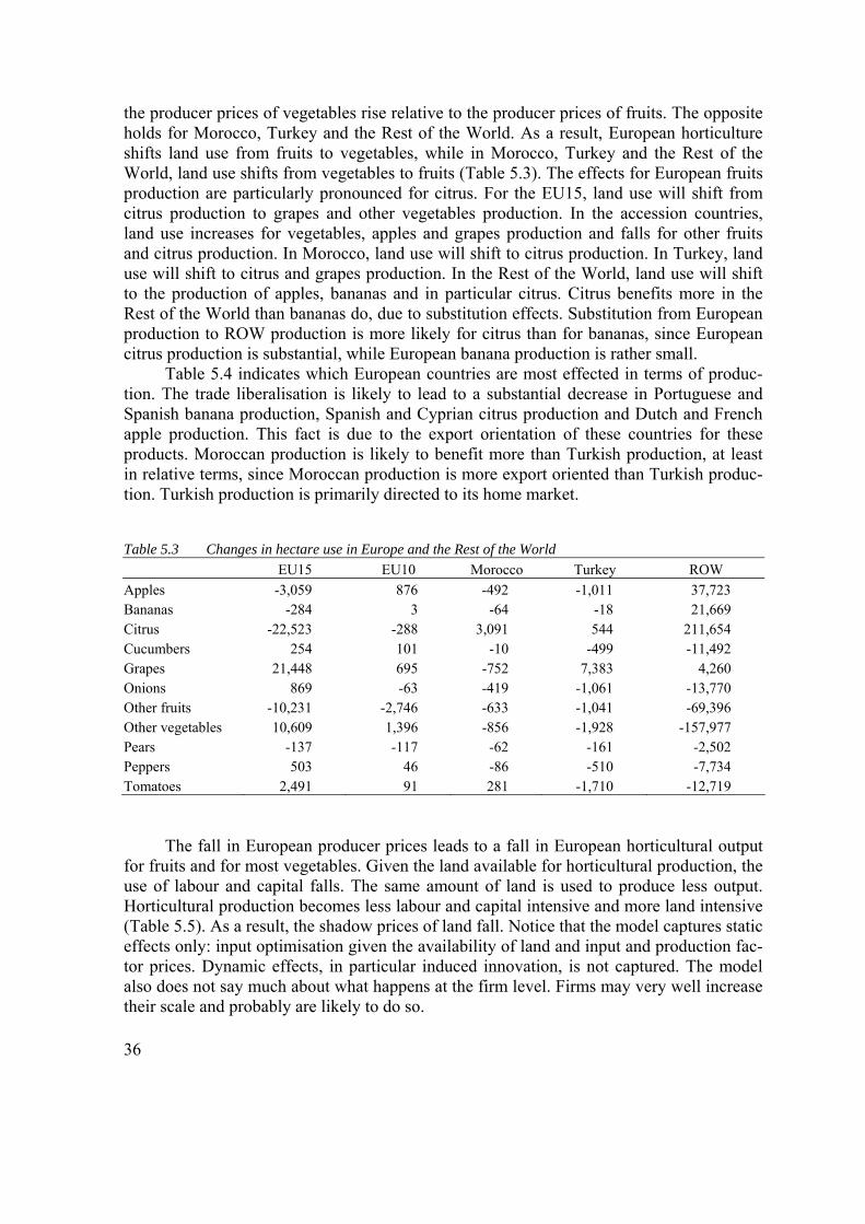
the producer prices of vegetables rise relative to the producer prices of fruits. The opposite holds for Morocco, Turkey and the Rest of the World. As a result, European horticulture shifts land use from fruits to vegetables, while in Morocco, Turkey and the Rest of the World, land use shifts from vegetables to fruits (Table 5.3). The effects for European fruits production are particularly pronounced for citrus. For the EU15, land use will shift from citrus production to grapes and other vegetables production. In the accession countries, land use increases for vegetables, apples and grapes production and falls for other fruits and citrus production. In Morocco, land use will shift to citrus production. In Turkey, land use will shift to citrus and grapes production. In the Rest of the World, land use will shift to the production of apples, bananas and in particular citrus. Citrus benefits more in the Rest of the World than bananas do, due to substitution effects. Substitution from European production to ROW production is more likely for citrus than for bananas, since European citrus production is substantial, while European banana production is rather small.
Table 5.4 indicates which European countries are most effected in terms of produc-tion. The trade liberalisation is likely to lead to a substantial decrease in Portuguese and Spanish banana production, Spanish and Cyprian citrus production and Dutch and French apple production. This fact is due to the export orientation of these countries for these products. Moroccan production is likely to benefit more than Turkish production, at least in relative terms, since Moroccan production is more export oriented than Turkish produc-tion. Turkish production is primarily directed to its home market. Table 5.3 Changes in hectare use in Europe and the Rest of the World
EU15 EU10 Morocco Turkey ROW Apples -3,059 876 -492 -1,011 37,723 Bananas -284 3 -64 -18 21,669 Citrus -22,523 -288 3,091 544 211,654 Cucumbers 254 101 -10 -499 -11,492 Grapes 21,448 695 -752 7,383 4,260 Onions 869 -63 -419 -1,061 -13,770 Other fruits -10,231 -2,746 -633 -1,041 -69,396 Other vegetables 10,609 1,396 -856 -1,928 -157,977 Pears -137 -117 -62 -161 -2,502 Peppers 503 46 -86 -510 -7,734 Tomatoes 2,491 91 281 -1,710 -12,719
The fall in European producer prices leads to a fall in European horticultural output for fruits and for most vegetables. Given the land available for horticultural production, the use of labour and capital falls. The same amount of land is used to produce less output. Horticultural production becomes less labour and capital intensive and more land intensive (Table 5.5). As a result, the shadow prices of land fall. Notice that the model captures static effects only: input optimisation given the availability of land and input and production fac-tor prices. Dynamic effects, in particular induced innovation, is not captured. The model also does not say much about what happens at the firm level. Firms may very well increase their scale and probably are likely to do so.
36

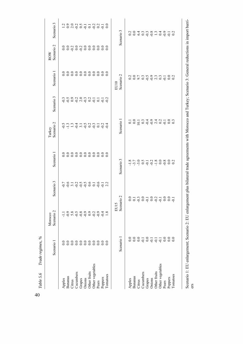
5.2 Trade regimes for fruits and vegetables The precise impact of trade liberalization depends among other things upon the countries included. Trade liberalisation is negotiated at regional (bilateral) and world levels. The EU is involved in regional trade negotiations and in global negotiations. The current EU enlargement may be seen as a regional negotiation. The same holds for negotiations with Mediterranean countries. WTO negotiations (with respect to bananas e.g.) are an example of global negotiations. Regional free trade agreements may lead to trade distortions, since trade may be di-verted from the countries which are not a partner to the agreement to countries which are. With respect to the EU enlargement, EU imports of oranges may be diverted from Brazil (Rest of the World) to Cyprus, since Cyprus is treated as a preferential trade partner, while Brazil is not. This hurts the international division of production and exports if Brazil is a more efficient producer than Cyprus is. Table 5.6 shows the effects of trade liberalisation under three scenarios. Scenario 1 refers to the current situation: EU enlargement. What happens to horticultural production now trade barriers between the EU and the new Member States are abolished? Note that the model data are from 2000, four years before the actual enlargement. Scenario 2 extends the EU enlargement in Scenario 1 with bilateral trade agreements with Morocco and Tur-key. This is a likely scenario for the near future: bilateral arrangements between the EU and the Mediterranean region. Scenario 3 may be considered as a benchmark, since the trade liberalization does not discriminate between countries. The difference between sce-nario 1 on one hand and 2 and 3 on the other hand and the difference between scenario 2 and 3 give indications of the importance of trade diversion. Scenario 3 has been analysed in detail in the previous section.
Table 5.6 shows that trade diversion is likely to occur for citrus. Morocco and Tur-key produce more citrus, but also less of all other fruits and vegetables, when they are treated preferentially. The rest of the world produces less citrus, when Morocco and Tur-key are treated preferentially. Trade diversion also arises, among other things, for Turkish grapes and Cyprian citrus. Trade diversion is not that important for the current EU enlargement (scenario 1). The EU 15 and the ROW are generally speaking hardly effected. However, there are countries that are substantially effected for one or more products, as Table 5.4 shows.
37

38
Tabl
e 5.
4 O
utpu
t cha
nges
, % c
hang
e
Aus
tria
Bel
Lux
Cyp
rus
Cze
chR
ep D
enm
ark
Esto
nia
Finl
and
Fran
ce
Ger
man
y G
reec
e H
unga
ry
Irel
and
Italy
La
tvia
A
pple
s -1
.39
-2.4
7 -2
.33
5.00
0
-0.9
2 -1
.62
-3.5
1 -0
.82
0.10
-1
.18
0 -1
.06
-1.4
0 B
anan
as
0 0
0 0
0 0
0 0
0 0
0 0
0 0
Citr
us
0 0
6.47
0
0 0
0 0
0 -0
.85
0 0
-0.7
1 0
Cuc
umbe
rs
-0.1
9 1.
07
-0.8
9 -1
.82
0.21
1.
40
0.79
0.
20
-0.0
1 0.
32
0.19
0.
54 -
0.11
0.
05
Gra
pes
0.14
0
-0.2
2 -0
.38
0 0
0 0.
07
-0.0
4 -1
.64
-0.5
1 0
-0.5
1 0
Oni
ons
-0.6
5 0
-0.9
8 -0
.87
-0.3
6 -1
.33
0.65
-0
.34
-0.8
6 0.
29
-0.8
0.
04 -
0.25
-0
.04
Oth
er fr
uits
-1
.42
0 -0
.36
-0.1
7 -2
.51
0 -2
.7
-2.8
3 -0
.95
-0.6
3 6.
63
-2.5
4 -1
.75
-0.7
8 O
ther
veg
etab
les
-0.2
3 -0
.59
1.68
-0
.47
-0.5
4 0.
62
0.76
-0
.10
0.13
0.
36
0.40
-0
.09
0.16
0.
60
Pear
s -0
.88
-2.3
1 -1
.35
-1.1
7 -0
.79
0 0
-1.8
0 -1
.37
-0.7
1 -0
.11
0 -0
.68
-0.9
0 Pe
pper
s 0
-0.3
2 -1
.05
-3.3
9 0
0 0
0 0
0.26
0.
71
0.15
0.
12
0 To
mat
oes
-0.2
3 0.
19
-1.4
4 -0
.03
-1.2
2 -0
.15
0.25
-0
.12
-1.0
1 0.
37
0.39
0.
49
0.23
-0
.07
Li
thua
nia
Mal
ta
Mor
occo
N
ethe
rland
s Po
land
Po
rtuga
l R
OW
Sl
ovak
Rep
Sl
oven
ia
Spai
n Sw
eden
Tu
rkey
U
K
App
les
-0.6
9 0
-0.6
6 -3
.32
0 -0
.82
1.21
-0
.97
-0.2
9 0.
22
-2.6
1 -0
.34
-2.8
6 B
anan
as
0 0
-0.5
5 0
0 -7
.88
0.92
0
0 -3
.44
0 -0
.45
0 C
itrus
0
-0.1
0 3.
08
0 0
-0.8
7 2.
01
0 0
-4.9
4 0
0.87
0
Cuc
umbe
rs
2.47
0
-0.1
8 0.
38
0.18
0.
22
-0.1
9 3.
73
-1.4
0 0.
99
0.58
-0
.20
0.55
G
rape
s 0
-0.4
9 -0
.49
0 0
0.16
0.
52
1.37
-0
.28
0.35
0
1.95
0
Oni
ons
-0.0
3 0
-0.5
3 -0
.02
2.51
0.
23
-0.1
1 0.
6 -0
.85
0.73
0.
39
-0.2
9 0.
53
Oth
er fr
uits
-1
.64
-1.1
3 0.
58
0 0.
81
-0.9
7 0.
07
-1.1
2 4.
15
-2.9
0 -3
.16
0.15
-3
.17
Oth
er v
eget
able
s 0.
57
0 0.
11
-0.3
6 0.
19
0.19
-0
.17
0.8
1.70
0.
38
0.43
-0
.11
0.31
Pe
ars
-1.1
5 -0
.32
-0.5
5 -2
.53
-0.8
2 -1
.21
0.22
-3
.17
-0.5
1 -0
.01
-2.1
3 0.
13
-1.9
5 Pe
pper
s 0
0 -0
.06
-0.5
2 0
0 -0
.14
-0.6
8 0
0.28
0
-0.1
1 0.
12
Tom
atoe
s 6.
00
0 2.
17
-0.6
2 0.
10
0.17
0.
03
2.05
0
0.44
0.
24
-0.1
7 0.
71

39
Tabl
e 5.
5 D
eman
d fo
r lab
our a
nd c
apita
l, %
cha
nge
Aus
tria
Bel
Lux
Cyp
rus
Cze
chR
ep D
enm
ark
Esto
nia
Finl
and
Fran
ce
Ger
man
y G
reec
e H
unga
ry
Irel
and
Italy
La
tvia
A
pple
s -1
.58
-2.9
4 -1
.52
5.49
0
-1.0
7 -2
.02
-3.6
7 -1
.03
-0.2
5 -0
.52
0 -1
.32
-1.6
5 B
anan
as
0 0
0 0
0 0
0 0
0 0
0 0
0 0
Citr
us
0 0
7.28
0
0 0
0 0
0 -1
.20
0 0
-0.9
7 0
Cuc
umbe
rs
-0.3
8 0.
60
-0.0
9 -1
.33
-0.3
0 1.
26
0.40
0.
04
-0.2
2 -0
.03
0.85
0.
32 -
0.37
-0.
20
Gra
pes
-0.0
5 0
0.58
0.
11
0 0
0 -0
.09
-0.2
6 -1
.99
0.15
-0
.22
-0.7
6 0
Oni
ons
-0.8
4 0
-0.1
8 -0
.38
-0.8
7 -1
.48
0.25
-0
.50
-1.0
7 -0
.06
-0.1
4 -0
.18
-0.5
1 -0
.29
Oth
er fr
uits
-1
.60
0 0.
45
0.32
-3
.02
0 -3
.10
-2.9
9 -1
.17
-0.9
8 7.
29
-2.7
6 -2
.01
-1.0
3 O
ther
veg
etab
les
-0.4
2 -1
.06
2.49
0.
02
-1.0
5 0.
47
0.36
-0
.26
-0.0
9 0.
01
1.06
-0
.31
-0.0
9 0.
36
Pear
s -1
.07
-2.7
9 -0
.54
-0.6
8 -1
.30
0 0
-1.9
7 -1
.58
-1.0
6 0.
55
0 -0
.93
-1.1
5 Pe
pper
s 0
-0.8
0 -0
.24
-2.9
0 0
0 0
0 0
-0.0
9 1.
37
-0.0
7 -0
.13
0 To
mat
oes
-0.4
2 -0
.29
-0.6
4 0.
46
-1.7
3 -0
.30
-0.1
4 -0
.28
-1.2
3 0.
02
1.05
0.
27 -
0.03
-0.
31
Li
thua
nia
Mal
ta
Mor
occo
N
ethe
rland
s Po
land
Po
rtuga
l R
OW
Sl
ovak
Rep
Sl
oven
ia
Spai
n Sw
eden
Tu
rkey
U
K
App
les
-0.8
2 0
-0.1
1 -3
.73
0.21
-0
.98
1.41
-0
.66
-0.2
0 -0
.44
-2.9
0 -0
.05
-3.0
0 B
anan
as
0 0
0.00
0
0 -8
.04
1.12
0
0 -4
.10
0 -0
.16
0 C
itrus
0
-0.2
5 3.
62
0 0
-1.0
2 2.
21
0 0
-5.6
0 0
1.16
0
Cuc
umbe
rs
2.34
0
0.37
-0
.04
0.39
0.
07
0.01
4.
04
-1.3
1 0.
33
0.29
0.
08
0.40
G
rape
s 0
-0.6
3 0.
06
0 0
0.00
0.
72
1.67
-0
.20
-0.3
1 0
2.24
0
Oni
ons
-0.1
6 0
0.01
-0
.43
2.72
0.
07
0.09
0.
9 -0
.77
0.07
0.
09
-0.0
1 0.
38
Oth
er fr
uits
-1
.77
-1.2
7 1.
12
0 1.
03
-1.1
2 0.
27
-0.8
2 4.
23
-3.5
6 -3
.45
0.43
-3.
32
Oth
er v
eget
able
s 0.
44
0 0.
65
-0.7
8 0.
40
0.04
0.
03
1.11
1.
78
-0.2
8 0.
14
0.17
0.
16
Pear
s -1
.28
-0.4
6 0.
00
-2.9
4 -0
.61
-1.3
6 0.
42
-2.8
6 -0
.43
-0.6
6 -2
.42
0.42
-2.
10
Pepp
ers
0 0
0.48
-0
.93
0 0
0.06
-0
.37
0 -0
.38
0 0.
18 -
0.03
To
mat
oes
5.87
0
2.71
-1
.03
0.32
0.
02
0.23
2.
36
0 -0
.21
-0.0
5 0.
11
0.56
40
Tabl
e 5.
6 Tr
ade
regi
mes
, %
Mor
occo
Tu
rkey
R
OW
Sc
enar
io 1
Sc
enar
io 2
Sc
enar
io 3
Sc
enar
io 1
Sc
enar
io 2
Sc
enar
io 3
Sc
enar
io 1
Sc
enar
io 2
Sc
enar
io 3
A
pple
s 0.
0 -1
.1
-0.7
0.
0 -0
.5
-0.3
0.
0 0.
0 1.
2 B
anan
as
0.0
-0.9
-0
.6
0.0
-1.3
-0
.5
0.0
0.0
0.9
Citr
us
0.0
5.8
3.1
0.0
1.3
0.9
0.0
-0.2
2.
0 C
ucum
bers
0.
0 -0
.5
-0.2
0.
0 -0
.4
-0.2
0.
0 0.
0 -0
.2
Gra
pes
0.0
-0.8
-0
.5
0.0
3.1
2.0
0.0
-0.2
0.
5 O
nion
s 0.
0 -0
.9
-0.5
0.
0 -0
.5
-0.3
0.
0 0.
0 -0
.1
Oth
er fr
uits
0.
0 0.
9 0.
6 0.
0 0.
2 0.
2 0.
0 0.
0 0.
1 O
ther
veg
etab
les
0.0
-0.2
0.
1 0.
0 -0
.3
-0.1
0.
0 0.
0 -0
.2
Pear
s 0.
0 -0
.9
-0.6
0.
0 0.
1 0.
1 0.
0 0.
0 0.
2 Pe
pper
s 0.
0 -0
.4
-0.1
0.
0 -0
.2
-0.1
0.
0 0.
0 -0
.1
Tom
atoe
s 0.
0 1.
8 2.
2 0.
0 -0
.4
-0.2
0.
0 0.
0 0.
0
EU
15
EU
10
Sc
enar
io 1
Sc
enar
io 2
Sc
enar
io 3
Sc
enar
io 1
Sc
enar
io 2
Sc
enar
io 3
A
pple
s 0.
0 0.
0 -1
.8
0.1
0.2
0.2
Ban
anas
0.
0 0.
1 -3
.7
0.0
0.0
0.0
Citr
us
0.0
-0.3
-3
.0
10.1
9.
7 6.
4 C
ucum
bers
-0
.1
0.0
0.5
0.3
0.3
0.3
Gra
pes
0.0
-0.1
-0
.1
-0.4
-0
.5
-0.3
O
nion
s -0
.1
0.0
-0.2
-0
.9
-0.9
-0
.8
Oth
er fr
uits
-0
.1
-0.2
-1
.8
2.4
2.3
1.3
Oth
er v
eget
able
s -0
.1
-0.1
0.
0 0.
2 0.
3 0.
4 Pe
ars
0.0
0.0
-0.8
-0
.1
-0.1
-0
.9
Pepp
ers
0.0
0.0
0.0
0.0
0.0
-0.1
To
mat
oes
0.0
-0.1
0.
2 0.
3 0.
2 0.
2 Sc
enar
io 1
: EU
enl
arge
men
t; Sc
enar
io 2
: EU
enl
arge
men
t plu
s bila
tera
l tra
de a
gree
men
ts w
ith M
oroc
co a
nd T
urke
y; S
cena
rio 3
: Gen
eral
redu
ctio
ns in
impo
rt ba
rri-
ers
5.3 A rise in Dutch energy costs This section presents the results of a second simulation: an increase in energy costs in the Netherlands. Energy costs would rise in the Netherlands, if the Netherlands would sharpen its energy or climate policy unilaterally. A rise in energy costs in the Netherlands with 25% would lead to an increase in the price index of intermediary inputs with 10%. The energy price rise is modelled by raising the price of intermediary inputs with 10% for all glass-house crops (cucumbers, sweet peppers, ornamental flowers and tomatoes) and with 5% for nursery material (pot plants and nursery material). All other products are not affected. In the analysis we will pinpoint out attention on the competitive position of Dutch glass-house vegetables versus Dutch ornamentals. Producer prices The rise in prices of intermediates increases producer prices in the Netherlands (Table 5.7). Naturally, this increase is more pronounced for ornamental flowers and glasshouse vegeta-bles than for nursery plants, since the price increase modelled was lower for the latter. For reasons beyond the scope of this article, the increase in producer prices of nursery plants is counterbalanced by an increase in the availability of land formerly occupied by ornamen-tals and glasshouse vegetables sectors. Producer prices increase more for ornamental flowers than they do for glasshouse vegetables, since producers of ornamental flowers are better able to pass on cost increases to consumers. Dutch ornamental flower producers face less competition than producers of glasshouse vegetables do. Table 5.7 Changes in producer prices in the Netherlands, % change Apples -0.40 Bananas -0.40 Citrus -0.40 Cucumbers 4.24 Grapes -0.40 Nursery Plants 0.70 Onions -0.27 Ornamental flowers 4.79 Other Fruits -0.40 Other Vegetables -0.27 Pears -0.40 Peppers 4.24 Tomatoes 4.09 Land use We notice that land used for the production of both glasshouse vegetables and ornamentals decreases considerably in the Netherlands. As expected, the burden falls more heavily on vegetables than on ornamentals flowers. Dutch producers of glasshouse vegetables face more competition and more actual substitution than Dutch producers of ornamental flowers do. For this reason, Dutch producers switch from glasshouse vegetables to ornamental flowers and nursery material, including pot plants. Tomatoes are affected relatively badly,
41

42
since they face fiercer competition on the respective import markets than cucumber and pepper producers do (See Table 5.8). Table 5.8 Absolute changes in land use, hectares (% change between brackets) Netherlands Spain Rest
EU-15New EU members
Morocco Turkey Rest of the World
Apples 263 (2.05) -29 (-0.06) -215 -93 -3 -11 -943Bananas 0 -4 (-0.05) 0 0 0 0 -417Citrus 0 -526 (-0.09) 0 -1 -31 -18 -1298Cucumbers -69 (-10.51) 343 (4.83) 116 51 0 13 390Grapes 0.3 (0.79) -447 (-0.04) -43 -16 0 -54 0Nursery material 115 (1.01) -0.4 (-0.02) -194 -8 0 -1 0Onions 189 (1.43) -14 (-0.06) 18 -28 0 -12 0Ornamentals -1,189 (-4.52) 23 (0.42) 95 14 9 14 150Other fruits 40 (0.79) -215 (-0.08) -262 -64 -12 -25 0Other vegetables 821 (1.47) -107 (-0.05) 384 11 -9 0 0Pears 121 (2.01) -36 (-0.09) -75 -7 0 -4 -139Peppers -144 (-11.98) 436 (1.88) 40 60 4 45 859Tomatoes -146 (-12.92) 512 (0.85) 160 82 34 68 1719 Sector output Table 5.9 and 5.10 present the results of the energy price increase for sectoral output and demand for intermediate inputs, and demand for labour and capital in all regions. These ta-bles describe in detail what happens to production and consumption. The results show that in terms of production tomato producers are worse off than producers of ornamental flow-ers and other glasshouse vegetables. This result might seem peculiar, because producer prices of tomatoes increase less than those of the other affected products. We can explain this fact by looking at the economic structure of the model. There are at least two explana-tions.
First, why does vegetables' output decline more than ornamental output? Exporters of ornamentals face less competition and are better able to pass on price increases. In other words, in vegetable markets there are more suppliers and consequently the increase in Dutch export prices is more pronounced vis-à-vis average export prices of its competitors.
Second, why are tomato producers in a less favourable position than cucumber or pepper producers? This is partly explained by the fact that the Dutch export ratio is higher for tomatoes than it is for the other two products. However, the difference is small, the ex-port ratio is 81% for tomatoes, against 79 and 75% for peppers and cucumbers respectively. However, Dutch tomato producers face more competition from foreign - i.e. Spanish - producers than cucumber and pepper producers do, especially in Germany, Neth-erlands' most important export market. Dutch exporters have a market share above 50% for cucumbers, but only a 33% market share for tomatoes.
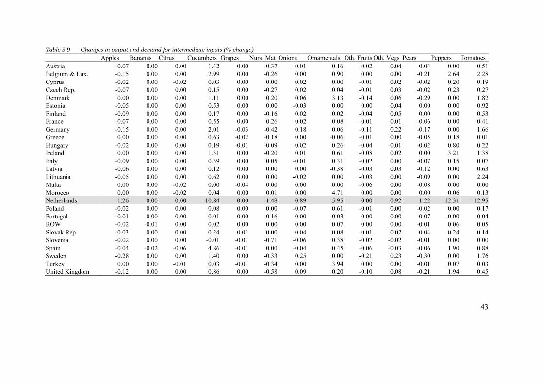
Table 5.9 Changes in output and demand for intermediate inputs (% change) Apples Bananas Citrus Cucumbers Grapes Nurs. Mat Onions Ornamentals Oth. Fruits Oth. Vegs Pears Peppers Tomatoes Austria -0.07 0.00 0.00 1.42 0.00 -0.37 -0.01 0.16 -0.02 0.04 -0.04 0.00 0.51Belgium & Lux.
-0.15 0.00 0.00 2.99 0.00 -0.26 0.00 0.90 0.00 0.00 -0.21 2.64 2.28
Cyprus -0.02 0.00 -0.02 0.03 0.00 0.00 0.02 0.00 -0.01 0.02 -0.02 0.20 0.19
Czech Rep. -0.07 0.00 0.00 0.15 0.00 -0.27 0.02 0.04 -0.01 0.03 -0.02 0.23 0.27 Denmark 0.00 0.00 0.00 1.11 0.00 0.20 0.06 3.13 -0.14 0.06 -0.29 0.00 1.82Estonia -0.05 0.00 0.00 0.53 0.00 0.00 -0.03 0.00 0.00 0.04 0.00 0.00 0.92Finland -0.09 0.00 0.00 0.17 0.00 -0.16 0.02 0.02 -0.04 0.05 0.00 0.00 0.53France -0.07 0.00 0.00 0.55 0.00 -0.26 -0.02 0.08 -0.01 0.01 -0.06 0.00 0.41Germany -0.15 0.00 0.00 2.01 -0.03 -0.42 0.18 0.06 -0.11 0.22 -0.17 0.00 1.66Greece 0.00 0.00 0.00 0.63 -0.02 -0.18 0.00 -0.06 -0.01 0.00 -0.05 0.18 0.01 Hungary -0.02 0.00 0.00 0.19 -0.01 -0.09 -0.02 0.26 -0.04 -0.01 -0.02 0.80 0.22Ireland 0.00 0.00 0.00 1.31 0.00 -0.20 0.01 0.61 -0.08 0.02 0.00 3.21 1.38Italy -0.09 0.00 0.00 0.39 0.00 0.05 -0.01 0.31 -0.02 0.00 -0.07 0.15 0.07Latvia -0.06 0.00 0.00 0.12 0.00 0.00 0.00 -0.38
-0.03 0.03 -0.12 0.00 0.63
Lithuania -0.05 0.00 0.00 0.62 0.00 0.00 -0.02 0.00 -0.03 0.00 -0.09 0.00 2.24Malta 0.00 0.00 -0.02 0.00 -0.04 0.00 0.00 0.00 -0.06 0.00 -0.08 0.00 0.00Morocco 0.00 0.00 -0.02 0.04 0.00 0.01 0.00 4.71 0.00 0.00 0.00 0.06 0.13Netherlands 1.26 0.00 0.00 -10.84 0.00 -1.48 0.89 -5.95 0.00 0.92 1.22 -12.31 -12.95 Poland
-0.02 0.00 0.00 0.08 0.00 0.00 -0.07 0.61 -0.01 0.00 -0.02 0.00 0.17Portugal -0.01 0.00 0.00 0.01 0.00 -0.16 0.00 -0.03 0.00 0.00 -0.07 0.00 0.04ROW -0.02 -0.01 0.00 0.02 0.00 0.00 0.00 0.07 0.00 0.00 -0.01 0.06 0.05Slovak Rep. -0.03 0.00 0.00 0.24 -0.01 0.00 -0.04 0.08 -0.01 -0.02 -0.04 0.24 0.14 Slovenia -0.02 0.00 0.00 -0.01 -0.01 -0.71 -0.06 0.38 -0.02 -0.02 -0.01 0.00 0.00Spain -0.04 -0.02 -0.06 4.86 -0.01 0.00 -0.04 0.45 -0.06 -0.03 -0.06 1.90 0.88Sweden -0.28 0.00 0.00 1.40 0.00 -0.33 0.25 0.00 -0.21 0.23 -0.30 0.00 1.76Turkey 0.00 0.00 -0.01 0.03 -0.01 -0.34 0.00 3.94 0.00 0.00 -0.01 0.07 0.03United Kingdom -0.12 0.00 0.00 0.86 0.00 -0.58 0.09 0.20 -0.10 0.08 -0.21 1.94 0.45
43
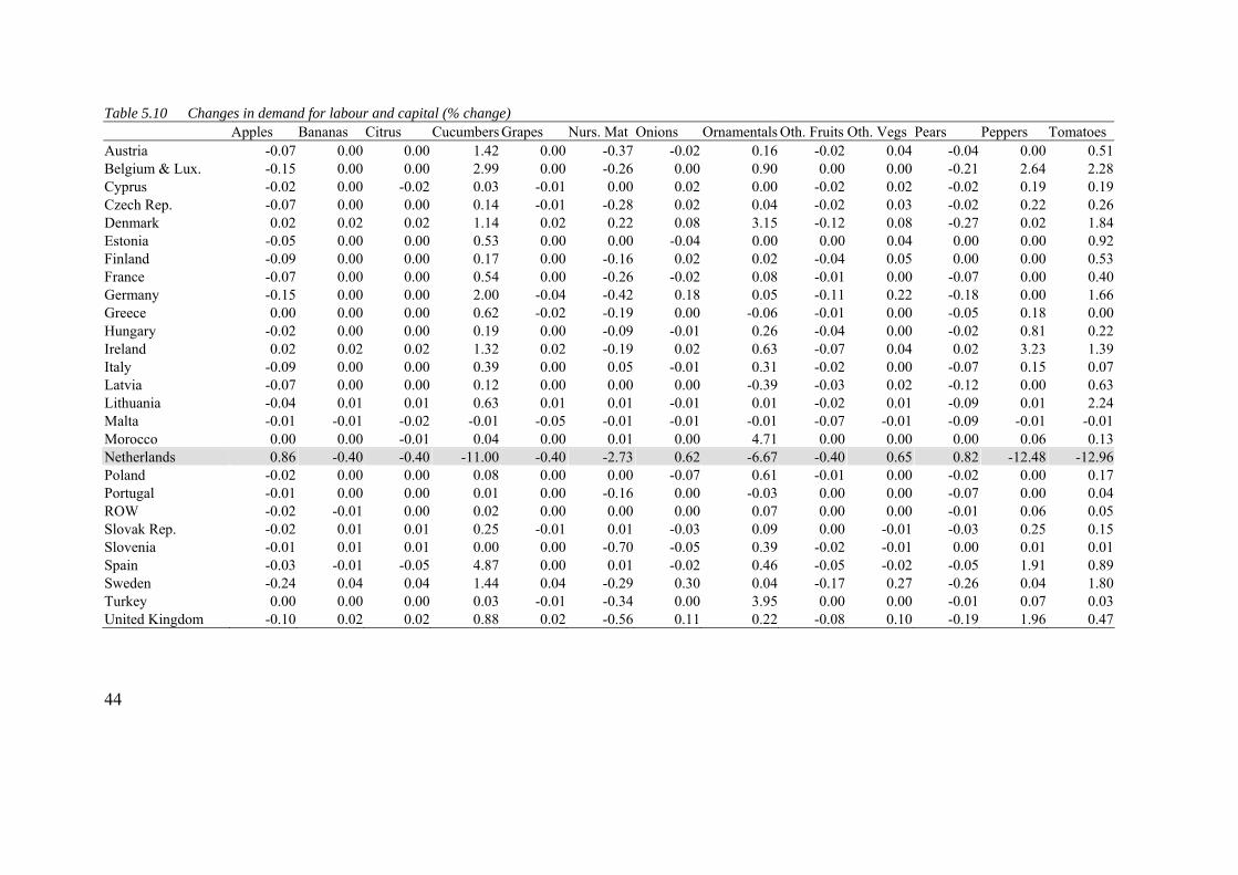
Table 5.10 Changes in demand for labour and capital (% change) Apples Bananas Citrus Cucumbers Grapes Nurs. Mat Onions Ornamentals Oth. Fruits Oth. Vegs Pears Peppers Tomatoes Austria -0.07 0.00 0.00 1.42 0.00 -0.37 -0.02 0.16 -0.02 0.04 -0.04 0.00 0.51Belgium & Lux.
-0.15 0.00 0.00 2.99 0.00 -0.26 0.00 0.90 0.00 0.00 -0.21 2.64 2.28
Cyprus -0.02 0.00 -0.02 0.03 -0.01 0.00 0.02 0.00 -0.02 0.02 -0.02 0.19 0.19
Czech Rep. -0.07 0.00 0.00 0.14 -0.01 -0.28 0.02 0.04 -0.02 0.03 -0.02 0.22 0.26 Denmark 0.02 0.02 0.02 1.14 0.02 0.22 0.08 3.15 -0.12 0.08 -0.27 0.02 1.84Estonia -0.05 0.00 0.00 0.53 0.00 0.00 -0.04 0.00 0.00 0.04 0.00 0.00 0.92Finland -0.09 0.00 0.00 0.17 0.00 -0.16 0.02 0.02 -0.04 0.05 0.00 0.00 0.53France -0.07 0.00 0.00 0.54 0.00 -0.26 -0.02 0.08 -0.01 0.00 -0.07 0.00 0.40Germany -0.15 0.00 0.00 2.00 -0.04 -0.42 0.18 0.05 -0.11 0.22 -0.18 0.00 1.66Greece 0.00 0.00 0.00 0.62 -0.02 -0.19 0.00 -0.06 -0.01 0.00 -0.05 0.18 0.00 Hungary -0.02 0.00 0.00 0.19 0.00 -0.09 -0.01 0.26 -0.04 0.00 -0.02 0.81 0.22Ireland 0.02 0.02 0.02 1.32 0.02 -0.19 0.02 0.63 -0.07 0.04 0.02 3.23 1.39Italy -0.09 0.00 0.00 0.39 0.00 0.05 -0.01 0.31 -0.02 0.00 -0.07 0.15 0.07Latvia -0.07 0.00 0.00 0.12 0.00 0.00 0.00 -0.39 -0.03 0.02 -0.12 0.00 0.63Lithuania -0.04 0.01 0.01 0.63 0.01 0.01 -0.01 0.01 -0.02 0.01 -0.09 0.01 2.24Malta -0.01 -0.01 -0.02 -0.01 -0.05 -0.01 -0.01 -0.01 -0.07 -0.01 -0.09 -0.01 -0.01Morocco 0.00 0.00 -0.01 0.04 0.00 0.01 0.00 4.71 0.00 0.00 0.00 0.06 0.13Netherlands 0.86 -0.40 -0.40 -11.00 -0.40 -2.73 0.62 -6.67 -0.40 0.65 0.82 -12.48 -12.96 Poland
-0.02 0.00 0.00 0.08 0.00 0.00 -0.07 0.61 -0.01 0.00 -0.02 0.00 0.17Portugal -0.01 0.00 0.00 0.01 0.00 -0.16 0.00 -0.03 0.00 0.00 -0.07 0.00 0.04ROW -0.02 -0.01 0.00 0.02 0.00 0.00 0.00 0.07 0.00 0.00 -0.01 0.06 0.05Slovak Rep. -0.02 0.01 0.01 0.25 -0.01 0.01 -0.03 0.09 0.00 -0.01 -0.03 0.25 0.15 Slovenia -0.01 0.01 0.01 0.00 0.00 -0.70 -0.05 0.39 -0.02 -0.01 0.00 0.01 0.01Spain -0.03 -0.01 -0.05 4.87 0.00 0.01 -0.02 0.46 -0.05 -0.02 -0.05 1.91 0.89Sweden -0.24 0.04 0.04 1.44 0.04 -0.29 0.30 0.04 -0.17 0.27 -0.26 0.04 1.80Turkey 0.00 0.00 0.00 0.03 -0.01 -0.34 0.00 3.95 0.00 0.00 -0.01 0.07 0.03United Kingdom -0.10 0.02 0.02 0.88 0.02 -0.56 0.11 0.22 -0.08 0.10 -0.19 1.96 0.47
44

6. Research agenda
This study makes a first step in developing an applied partial equilibrium model for Euro-pean horticulture. The model outlined in this study is made up of three elements: 1. A set of behavioural equations, more specifically:
- consumer demand for fruits, vegetables and ornamentals; - food industry demand for fruits and vegetables; - producer demand for intermediary inputs, land, labour and capital; - producer supply of fruits, vegetables and ornamentals;
2. A market clearing condition equating demand and supply of fruits, vegetables and ornamentals.
3. A database relating production, trade and consumption of fruits, vegetables and or-namentals. More specifically the database contains: - supply balance sheets, in tonnes, relating production, imports, exports, human
consumption and other uses for every product and region identified (Table 6.1); - bilateral trade data consistent with aggregate imports and exports from the sup-
ply balance sheets; - producer and export prices. At this stage, only export prices are used in the
model; - cost shares of intermediary inputs, labour and capital and land use for every
product and region identified.
HORTUS specifies supply and demand for six fruits, five vegetables and two orna-mentals for 27 regions: the EU25, Morocco, Turkey and the Rest of the World. Morocco and Turkey are modelled for illustrative reasons, since trade relations with Mediterranean countries are expected to be an interesting policy area in the near future (Table 6.1). Fur-ther extension of the model with new countries and products is relatively straightforward. Whether such extensions are meaningful depends on future demand for research. Table 6.1 Product, country and inputs choice
Vegetables Fruit Ornamentals Countries Inputs Cucumbers Onions Sweet peppers Tomatoes Other vegetables
Apples Bananas Citrus Grapes Pears Other fruit
Ornamental flowers Nursery plants
EU-25 Morocco Turkey Rest of the World
Land (area) Intermediary inputs Labour Capital
45

HORTUS may be used to study the impact of changes in the environment of the hor-ticultural supply on the key economic variables in the supply chain. The environmental (exogenous) variables modelled in HORTUS are given in Table 6.2 together with the key economic (endogenous) variables. HORTUS may be used to determine the policy implica-tions of changes in environmental variables that may be influenced by public policy and enterprise strategy, e.g. import tariffs, energy taxes. HORTUS will be used as a building stone of the Baseline scenario framework devel-oped at LEI. The Baseline scenario generates a projection of the future development of Dutch agriculture and horticulture and the impact of major policy and environmental changes on these projections. HORTUS may be improved by extending and improving the underlying database. Underdeveloped in the HORTUS model are data on: - the price structure is weakly developed, since HORTUS only defines export prices.
Producer prices, market prices, import prices and consumer prices are not incorpo-rated in the model as yet (see section 3.2). This does not invalidate the model as such, since the model is built on a consistent set of supply balances in tonnes and primarily depends on reasonable estimates of price, income and substitution elastic-ities;
- the price, income and substitution elasticities used in the current version of the model are simply chosen. Literature and empirical research may be used to come to less ar-bitrary estimates. This does not invalidate the current model, since sensitivity analyses are relatively straightforward;
The quality of the data may be improved by relating information from the supply
balance sheets with information from other sources, notably information on consumer and industrial buying behaviour. The data on ornamentals require thorough investigating. The best way to guarantee the quality of the data required is co-operation within a consortium. Table 6.2 Exogenous and endogenous variables
Exogenous variables Endogenous variables Prices endowments and intermediary inputs Population Income per capita Technological growth Taxes and subsidies on consumption, imports, exports and production International transport costs Total acreage available for horticulture
Product prices on the following levels: produc-tion, market, exports, imports and consumption Production Bilateral trade Demand for land endowments and intermediary inputs Consumption and industrial use
46
References Badinger, H., Breuss, F. and Mahlberg, B. (2002). Welfare effects of the EU's common or-ganization of the market in bananas for EU member states. Journal of Common Market Studies 40: 515-526. Cioffi, A. and dell'Aquila, C. (2004). The effects of trade policies for fresh fruit and vege-tables of the European Union. Food Policy 29: 169-185. Hertel, Thomas W. and Marinos E. Tsigas, Structure of GTAP. Draft of Chapter 2: 'Struc-ture of GTAP,' published in T.W. Hertel (ed.), Global Trade Analysis: Modeling and Applications, Cambridge University Press, 1997.
47

48

Appendix 1 Definitions of supply balance elements Table A1 Definitions of commodity balance elements from different sources Information on: Faostat definition Eurostat definition Production Figures relate to the total domestic
production whether inside or out-side the agricultural sector, i.e. it includes non-commercial produc-tion and production from kitchen gardens. Unless otherwise indi-cated, production is reported at the farm level for crop (i.e. in the case of crops, excluding harvesting losses).
Usable production comprises all usable quantities comprised from the production process, including the quantities used for 'own con-sumption' by producers. Losses occurring during the production process are not included.
Imports and exports Cover all movements into/out of the country of the commodity in question. It includes commercial trade, food aid granted on specific terms, donated quantities and es-timates of unrecorded trade. As a general rule, figures are reported in terms of net weight, i.e. exclud-ing the weight of the container.
Data are taken from official exter-nal trade statistics entering or leaving the territory of the Community or circulating be-tween the territories of the Member States (intra-EU-trade).
Human Consumption Comprises the amounts of the commodity in question and of any commodity derived therefrom not further pursued in the food bal-ance sheet, available for human consumption during the reference period.
Quantities of products made available for human consumption in all forms: quantities consumed without further processing and quantities supplied by the distribu-tive trades and the food industry.
Processing The amounts used during the ref-erence period for manufacture of processed commodities which could not be converted back to their originating primary com-modities or which are part of a separate food groups (e.g., sugar, fats and oils, alcoholic beverages) are shown here.
Quantities of products used to produce a derived food product for which there is a specific bal-ance sheet.
Waste Comprises the amounts of the commodity in question and it's de-rivatives not further pursued in the balances, lost through waste at all stages between the level at which production is recorded and the household. Losses before and dur-ing harvest are excluded.
Losses arising subsequent to the production process, during trans-port, storage or packaging. They include quantities withdrawn from the market and made unfit for consumption.
Other uses Seed, Feed, Other uses Seeds, Animal Feed, Industrial uses
Source: UN/ECE Statistical Division, Handbook of Agricultural Statistics.
49

50
Appendix 2 Data availability Table B1.1 gives an overview of the data used to construct consistent commodity balances (in 1.000 tonnes) and the availability for the products and countries in the model. By put-ting the available data together we have been able to construct commodity balances for all products and countries included in the model. Table B1.1 Availability and use of data from Eurostat Agris and Faostat, 2000
Eurostat Agris Table Faostat Commodity bal-ances
Fao crops primary
Fao trade
Are
a
Prod
uctio
n
Usa
ble
prod
uctio
n
Impo
rts
Expo
rts
Con
sum
ptio
n
Proc
essi
ng
Prod
uctio
n
Impo
rts
Expo
rts
Con
sum
ptio
n
Man
ufac
turin
g
Are
a
Prod
uctio
n
Impo
rts
Expo
rts
EU-15 * * * * * * * * * * * * * * * * EU-25 from '02 * * * * * * * * * * * * * * * * Other countries - - - - - - - * * * * * * * * * Vegetables Cucumbers - - - - - - - - - - - - *1 *1 *1 *1
Onions - - - - - - - * * * * * * * * * Chillies/Peppers - - - - - - - - - - - - * * * * Tomatoes * * * * * * * * * * * * * * * * Fruits Apples * * * * * * * * * * * * * * * * Bananas - - - - - - - * * * * * * * * * Citrus - - - - - - - * * * * * * * * * Grapes - - - - - - - * * * * * * * * * Pears * * * * * * * - - - - - * * * * Ornamentals Ornamental flowers / plants * * * * * * * - - - - - - - - - Nursery material * * * * * * * - - - - - - - - - 1 Including Gherkins
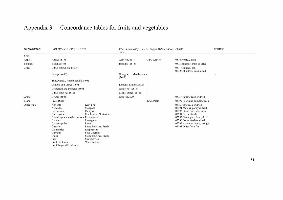
Appendix 3 Concordance tables for fruits and vegetables ITEMHORTUS FAO TRADE & PRODUCTION FAO Commodity Bal-
ance EU Supply Balance Sheets PCTAS COMEXT
Fruit Apples Apples (515) Apples (2617) APPL Apples 0574 Apples, fresh - Bananas
Bananas (486) Bananas (2615) - 0573 Bananas, fresh or dried - Citrus Citrus Fruit,Total (1804) - 0571 Oranges, etc.
0572 Oth.citrus, fresh, dried -
Oranges (490) Oranges, Mandarines(2611)
- -
Tang.Mand.Clement.Satsma (495) - - Lemons and Limes (497) Lemons, Limes (2612) - - Grapefruit and Pomelos (507) Grapefruit (2613) - - Citrus Fruit nes (512) Citrus, Other (2614) - - Grapes Grapes (560) Grapes (2620) - 0575 Grapes, fresh or dried - Pears Pears (521) - PEAR Pears 05792 Pears and quinces, fresh - Other fruits Apricots
Avocados Berries nes Blueberries Cantaloupes and other melonsCarobs Cashewapples Cherries Cranberries Currants Dates Figs Fruit Fresh nes Fruit Tropical Fresh nes
Kiwi Fruit Mangoes Papayas Peaches and Nectarines Persimmons Pineapples Plums Pome Fruit nes, Fresh Raspberries Sour Cherries Stone Fruit nes, Fresh Strawberries Watermelons
- - 0576 Figs, fresh or dried 05791 Melons, papayas, fresh 05793 Stone fruit, nes, fresh 05794 Berries fresh 05795 Pineapples, fresh, dried 05796 Dates, fresh or dried 05797 Avocado, guava, mango, 05798 Other fresh fruit
-
51
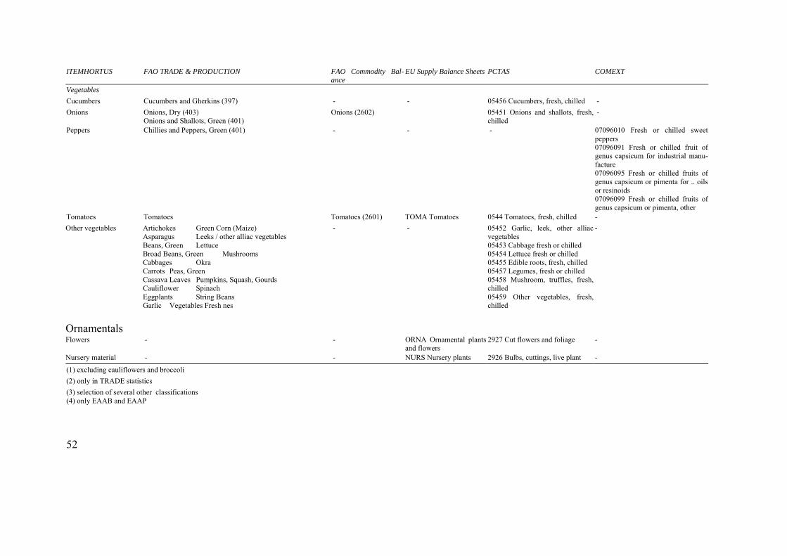
ITEMHORTUS
FAO TRADE & PRODUCTION FAO Commodity Bal-ance
EU Supply Balance Sheets PCTAS COMEXT
Vegetables Cucumbers Cucumbers and Gherkins (397) - - 05456 Cucumbers, fresh, chilled - Onions Onions, Dry (403)
Onions and Shallots, Green (401) Onions (2602) 05451 Onions and shallots, fresh,
chilled
-
Peppers Chillies and Peppers, Green (401) - - - 07096010 Fresh or chilled sweet peppers 07096091 Fresh or chilled fruit of genus capsicum for industrial manu-facture 07096095 Fresh or chilled fruits of genus capsicum or pimenta for .. oils or resinoids 07096099 Fresh or chilled fruits of genus capsicum or pimenta, other
Tomatoes
Tomatoes Tomatoes (2601) TOMA Tomatoes 0544 Tomatoes, fresh, chilled - Other vegetables Artichokes Green Corn (Maize)
Asparagus Leeks / other alliac vegetables Beans, Green Lettuce Broad Beans, Green Mushrooms Cabbages Okra Carrots Peas, Green Cassava Leaves Pumpkins, Squash, Gourds Cauliflower Spinach Eggplants String Beans Garlic Vegetables Fresh nes
- - 05452 Garlic, leek, other alliacvegetables
-
05453 Cabbage fresh or chilled 05454 Lettuce fresh or chilled 05455 Edible roots, fresh, chilled 05457 Legumes, fresh or chilled 05458 Mushroom, truffles, fresh, chilled 05459 Other vegetables, fresh, chilled
Ornamentals Flowers - - ORNA Ornamental plants
and flowers 2927 Cut flowers and foliage -
Nursery material - - NURS Nursery plants 2926 Bulbs, cuttings, live plant -
(1) excluding cauliflowers and broccoli (2) only in TRADE statistics (3) selection of several other classifications (4) only EAAB and EAAP
52