Advances in Water Resources 62 (2013) 254–265

Contents lists available at ScienceDirect

Advances in Water Resources

journal homepage: www.elsevier .com/ locate/advwatres

Homogenizability conditions for multicomponent reactive transport

0309-1708/$ - see front matter � 2013 Elsevier Ltd. All rights reserved.http://dx.doi.org/10.1016/j.advwatres.2013.07.014

⇑ Corresponding author.E-mail address: ibattia@clemson.edu (I. Battiato).

Francesca Boso a, Ilenia Battiato b,⇑a Department of Mechanical and Aerospace Engineering, University of California, San Diego, 9500 Gilman Dr., La Jolla, CA 92093, USAb Department of Mechanical Engineering, Clemson University, Clemson, SC 29634, USA

a r t i c l e i n f o

Article history:Available online 9 August 2013

Keywords:UpscalingHomogeneous reactionHeterogeneous reactionMulticomponent reactive transportDissolutionPrecipitation

a b s t r a c t

We consider multicomponent reactive transport in porous media involving three reacting species, two ofwhich undergo a nonlinear homogeneous reaction, while a third precipitates on the solid matrix througha heterogeneous nonlinear reaction. The process is fully reversible and can be described with a reaction ofthe kind Aþ B�C� S. The system’s behavior is fully controlled by Péclet (Pe) and three DamköhlerðDaj; j ¼ f1;2;3g) numbers, which quantify the relative importance of the four key mechanisms involvedin the transport process, i.e. advection, molecular diffusion, homogeneous and heterogeneous reactions.We use multiple-scale expansions to upscale the pore-scale system of equations to the macroscale, andestablish sufficient conditions under which macroscopic local advection–dispersion–reaction equations(ADREs) provide an accurate representation of the pore-scale processes. These conditions reveal that(i) the heterogeneous reaction leads to more stringent constraints compared to the homogeneous reac-tions, and (ii) advection can favorably enhance pore-scale mixing in the presence of fast reactions andrelatively low molecular diffusion. Such conditions are summarized by a phase diagram in the (Pe,Daj)-space, and verified through numerical simulations of multicomponent transport in a planar fracture withreacting walls. Our computations suggest that the constraints derived in our analysis are robust in iden-tifying sufficient as well as necessary conditions for homogenizability.

� 2013 Elsevier Ltd. All rights reserved.

1. Introduction

Nonlinear reactive transport in media with micro-structure isubiquitous to many environmental, industrial and biological sys-tems. While a majority of classical results in porous media theoryhave been obtained in the context of single- and multi-phase sub-surface transport [8,13,19], more effective recent investigationshave focused on biological systems, e.g. calcium dynamics in cellmembranes [12,18], and technological applications [4]. Otherapplications include chemical weathering, contaminant transportin aquifers [8], and geologic CO2 sequestration [27].

The plethora of scales involved in such systems allows one toemploy two general approaches in modeling transport phenom-ena: pore-scale or Darcy-scale (macroscopic, upscaled, continuum)models. Pore-scale simulations, e.g. pore-network models, latticeBoltzmann simulations [33], and particle methods [29], are basedon first principles, and therefore have strong physical foundations.Such models allow one to gain significant insight in the physicalprocess at the pore-scale. However, they require the knowledgeof pore-scale geometry at any location in the computational do-main, information seldom available in most applications. This ren-ders them impractical as a predictive tool at spatial and temporal

scales much larger than the pore-scale. Continuum-scale modelsare based on an effective medium representation of the systemwith effective transport parameters such as porosity, dispersioncoefficient, hydraulic conductivity, and effective reaction rates.Since upscaled models significantly alleviate computational bur-den, they are routinely used to model reaction processes at themacro-scale. However they rely on phenomenological descriptionsand/or closure assumptions which typically include geometricalconstraints that guarantee scale separation between the pore-and continuum-scales, linearization of pore-scale equations, andempirical closures, just to mention a few. These assumptions areoften necessary to fully decouple the pore-scale description andits continuum counterpart, and to obtain a local upscaled equation.Upscaling techniques - e.g. volume averaging [36], the methods ofmoments [11], homogenization [19] and its modifications to in-clude evolving microstructure [1,28], pore-network models, andthermodynamically constrained averaging [16] – allow one to for-mally establish the connection between pore- and continuum-scale models.

While Darcy’s law has proven to be very robust in modelingflow through porous media from the field- (i.e. kilometer-) to themicron-scale [3,4], the advection–dispersion-reaction equations(ADREs) fail to capture a number of observed transport features,including the extent of reactions in mixing-controlled chemicaltransformations [38] and asymmetrical long tails of breakthrough

F. Boso, I. Battiato / Advances in Water Resources 62 (2013) 254–265 255

curves [26], just to mention a few. Further, scale dependence ofeffective transport parameters [21,22] and discrepancy betweenlab and field experiments have long been recognized. They areattributed to concentration gradients and mass transport limita-tions at the pore-scale [24]. These shortcomings manifest them-selves when the approximations and/or closure assumptionsunderlying the continuum model are not fulfilled. Most upscalingstudies focus on the derivation of effective medium representa-tions for specific physical and geochemical processes [15, and ref-erences therein]. However, they rarely specify in which range ofparameters or physical regimes (e.g. diffusion- or reaction-con-trolled), such continuum-scale models are valid. Therefore, theapplication of macroscopic models to reactive systems with strongchemical/physical heterogeneity can be problematic since pore-scale reaction rates might exhibit a broad variability, and the trans-port process span significantly different regimes [38, and refer-ences therein].

The growing attention towards the mathematical foundationsof effective models and the connection between pore-scale pro-cesses and their representation at the continuum scale is reflectedby the increasing interest in modeling reactive transport at themicro-scale [9,29,33,37], and the concurrent development of mul-ti-algorithm (or hybrid) models which combine descriptions atdifferent scales [7,31,33]. In a number of works, e.g. [24,32],pore-scale simulations served as a tool to both gain insight in thephysical processes, and to verify the validity of macroscopic mod-els. Fewer are the works which have explicitly addressed the prob-lem of establishing conditions under which the pore-scaleprocesses correctly upscale to local macroscopic equations, e.g.[2,5,6,23,35]. Studies on the applicability range of macroscopicequations have involved the advection–dispersion equation(ADE) for conservative transport [2], the Taylor dispersion problemin a fracture with reactive walls [23], purely reactive–diffusivemulticomponent systems with nonlinear homogeneous reactions[6], and single component advective systems with nonlinear heter-ogeneous reactions [5]. The influence of mixing on the effectivereaction rate has had a long history in mathematics and engineer-ing, e.g. [14,38, and references therein].

In this work we generalize [5] by considering multicomponentreactive transport in porous media involving three reacting spe-cies, two of which undergo a nonlinear homogeneous reaction inthe liquid phase, while a third precipitates on the solid matrixthrough a heterogeneous nonlinear reaction at the solid–liquidinterface. The fully reversible biomolecular precipitation/dissolu-tion process can be described with a reaction of the typeAþ B�C� S. Calcite precipitation provides one example for thistype of reactions [24]. Additionally, numerical simulations of mul-ti-component reactive flow in a planar fracture are employed toverify the homogenizability conditions derived by multiple-scaleexpansions.

We start, in Section 2, by formulating a pore-scale model for thesystem under consideration, and by defining the dimensionlessPéclet (Pe) and three Damköhler ðDaj; j ¼ f1;2;3g) numbers whichquantify the relative importance of the four key mechanisms in-volved in the transport process, i.e. advection, molecular diffusion,homogeneous and heterogeneous reactions. In Section 3, by meansof multiple-scale expansions [19], we upscale the pore-scalesystem of equations to the macroscale, and establish sufficientconditions under which macroscopic local advection–dispersion–reaction equations (ADREs) provide an accurate representation ofpore-scale processes. Such conditions are summarized by a phasediagram in the (Pe,Daj)-space. Section 4 discusses a number of spe-cial cases. In Section 5 we verify the previously derived conditionsthrough pore-scale numerical simulations of multicomponenttransport in a planar fracture with reacting walls. Finally, the mainresults are summarized in the concluding Section 6.

2. Problem formulation

Consider reactive transport in a porous medium X whose char-acteristic length is L. Let us assume that the medium can be rep-resented microscopically by a collection of spatially periodic ‘‘unitcells’’ Y with a characteristic length ‘, and a scale parametere � ‘=L� 1. The unit cell Y ¼ B [ G consists of the pore space Band the impermeable solid matrix G, separated by the smoothsurface C. The pore spaces B of each cell Y form a multi-con-nected pore-space domain Be � X bounded by the smooth surfaceCe.

2.1. Governing equations

Let us assume the porous medium to be fully saturated with anincompressible fluid. Single-phase incompressible Stokes flow inthe pore-space Be is described by the Stokes and continuity equa-tions subject to the no-slip boundary condition on Ce,

mr2ve �rp ¼ 0; r � ve ¼ 0; x 2 Be; ve ¼ 0; x 2 Ce; ð1Þ

where veðxÞ is the fluid velocity, p denotes the fluid dynamic pres-sure, and m is the dynamic viscosity. The liquid is a solution of twochemical (or biological) species A and B (with concentrations aeðx; tÞand beðx; tÞ at point x 2 Be and time t, respectively) that react toform an aqueous reaction product C. Whenever ceðx; tÞ, the concen-tration of C, exceeds a threshold value c in proximity of a reactivewall, C undergoes a heterogeneous reaction and precipitates onthe solid matrix, forming a precipitate S. In general, this process isfully reversible, and its speed is controlled by the reaction rateskab; k; kc and kd corresponding to the following reactions,

Aþ B!kab C!k S and Aþ B kc C kd S: ð2Þ

The aqueous concentrations aeðx; tÞ; beðx; tÞ and ceðx; tÞ ½mol L�3 sat-isfy a system of advection–reaction–diffusion equations (ARDEs)

@ t ae ¼ r � ðDarae � veaeÞ � kabaebe þ kcce; x 2 Be; t > 0 ð3aÞ@ t be ¼ r � ðDbrbe � vebeÞ � kabaebe þ kcce; x 2 Be; t > 0 ð3bÞ@ t ce ¼ r � ðDcrce � veceÞ þ kabaebe � kcce; x 2 Be; t > 0; ð3cÞ

where the molecular diffusion coefficient Di, i ¼ fa; b; cg, is, in gen-eral, a positive-definite second-rank tensor. At the solid–liquidinterface Ce impermeable to flow, mass flux of the species C is bal-anced by the difference between the precipitation and dissolutionrates, Rp ¼ kcn

e and Rd ¼ kd, respectively [20]. Therefore,

�n � Dcrce ¼ kðcne � cnÞ; x 2 Ce; t > 0; ð4Þ

where n is the outward unit normal vector of Ce; k ½L3n�2T�1mol1�n�is the heterogeneous reaction rate constant, n 2 Zþ is related to theorder of reaction [25, Eq. 6] and the threshold concentrationcn ¼ kd=k represents the solubility product [25]. Due to precipita-tion on the solid–liquid interface, CeðtÞ evolves in time with velocityvs, according to qsvs � n ¼ kðcn

e � cnÞ, where qs is the molar densityof the precipitate [34]. In the following analysis, we disregard pre-cipitation-induced changes in pore geometry which occur on a timescale longer than the processes under investigation [6]. No-fluxboundary conditions hold for species A and B on the (multi-con-nected) liquid–solid interface Ce, i.e.

n � ðDaraeÞ ¼ n � ðDbrbeÞ ¼ 0: ð5Þ

Further, the flow and transport equations (1) and (3) are supple-mented with proper boundary conditions on the external boundaryof the flow domain X and with the initial conditions

aeðx;0Þ ¼ ainðxÞ; beðx;0Þ ¼ binðxÞ; ceðx;0Þ ¼ cinðxÞ: ð6Þ

256 F. Boso, I. Battiato / Advances in Water Resources 62 (2013) 254–265

Specifically, we consider a scenario in which reactants A and B, withinitial concentrations ain > 0 and bin > 0 respectively, are initially(i.e. t < 0) separated in space, and brought in contact with eachother at time t ¼ 0. Therefore the initial concentration of reactionproduct C is cin ¼ 0. Such initial distribution of the three specieshas the advantage of amplifying the reactions occurring along thereactive walls since cin – c, and inducing the formation of a local-ized reacting front.

2.2. Dimensionless formulation

For the sake of simplicity, we assume that the three reactingspecies A, B and C have the same diffusion coefficient, i.e.Da ¼ Db ¼ Dc ¼ D. We introduce the following dimensionlessquantities

ae ¼ae

cH; be ¼

be

cH; ce ¼

ce

c; D ¼ DD0

; x ¼ xL; ve ¼

ve

U;

p ¼ p‘2

mUL; ð7Þ

where U;D0 and cH ¼ maxfain; bing are characteristic values of ve;Dand the concentration of the reactants A and B, respectively. Properrescaling of pressure p ensures that the pressure gradient has thesame order of magnitude of the viscous term, as prescribed byStokes equation [2, Eqs. 15, 16]. Furthermore, the following timescales can be defined

td ¼L2

D0; ta ¼

LU; tr1 ¼

Lk�cn�1 ; tr2 ¼

1kabcH

; tr3 ¼1kc; ð8Þ

where td and ta are the time scales associated to diffusion andadvection. The three reactions, i.e. heterogeneous, nonlinear homo-geneous and linear homogeneous reactions, are described by thetime scales tr1; tr2 and tr3, respectively. Ratios between these timescales define the dimensionless Péclet (td=ta) and Damköhler(td=trj; j ¼ f1;2;3g) numbers,

Pe ¼ ULD0

; Da1 ¼LkD0

cn�1; Da2 ¼L2kab

D0cH; Da3 ¼

L2kc

D0ð9Þ

Rewriting (1), (2) and (3) in terms of the dimensionless quantities(7) and the dimensionless time t ¼ t=td yields a dimensionless formof the flow equations

e2r2ve �rp ¼ 0; r � ve ¼ 0; x 2 Be; ð10Þ

subject to

ve ¼ 0; x 2 Ce ð11Þ

and of the transport equations

@tae þr � �Drae þ Peveaeð Þ ¼ �Da2aebe þ gDa3ce; ð12aÞ@tbe þr � �Drbe þ Pevebeð Þ ¼ �Da2aebe þ gDa3ce; ð12bÞ@tce þr � �Drce þ Peveceð Þ ¼ g�1Da2aebe � Da3ce; ð12cÞ

where g ¼ �c=cH. The system (12) is subject to

n �Drae ¼ n �Drbe ¼ 0; �n �Drce ¼Da1 cne �1

� �; x 2Ce; t > 0:

ð13Þ

The initial conditions read

aeðx;0Þ ¼ ainðxÞ; beðx;0Þ ¼ binðxÞ; ceðx; 0Þ ¼ cinðxÞ: ð14Þ

3. Homogenization via multiple-scale expansions

We proceed by employing the method of multiple-scale expan-sions [2,19] to homogenize (upscale) the transport equations (10),(11), (12a)–(12c), (13) from the pore-scale to the macro-scale, and

to derive effective equations for the average flow velocity hveðxÞiand solutes’ concentrations haeðx; tÞi; hbeðx; tÞi, and hceðx; tÞi.

In Section 3.1 we provide the relevant definitions and thegeneral framework of the upscaling procedure. While the techni-cal details of the derivation are presented in Appendix, the re-sults of the homogenization procedure are summarized inSection 3.2. Here, we present a phase diagram identifying condi-tions under which the upscaled (macroscopic) system of equa-tions is valid.

3.1. Preliminaries

Given any pore-scale quantity we,

hwei �1jY j

ZBðxÞ

wedy; hweiB �1jBj

ZBðxÞ

wedy; and

hweiC �1jCj

ZCðxÞ

wedy ð15Þ

are three local averages (function of x) over the pore space BðxÞ ofthe unit cell YðxÞ centred at x. In (15), hwei ¼ /hweiB and / ¼ jBj=jY jis the porosity.

Within the framework of multiple-scale expansions method, weintroduce a space variable y defined in the unit cell, i.e. y 2 B, andfour time variables. One of the four time variables is related to theadvection time scale sa, while three are associated with the reac-tions time scales. The latter are represented by the vector sr withcomponents ½sr�j ¼ srj; j ¼ f1;2;3g. Each variable is defined asfollows,

y ¼ e�1x; sa ¼ Pe t ¼ t�1a t; and srj ¼ Daj t ¼ t�1

rj t; j ¼ f1;2;3g:ð16Þ

Furthermore, any pore-scale function weðx; tÞ (e.g. concentration in(12)) is represented as we x; tð Þ :¼ wðx; y; t; sa; srÞ. Replacing we x; tð Þwith wðx; y; t; sa; srÞ gives the following relations for the spatialand temporal derivatives,

rwe ¼ rxwþ e�1ryw; and@we

@t¼ @w@tþ Pe

@w@saþ Daj

@w@srj

; j ¼ f1;2;3g; ð17Þ

respectively, where Einstein summation is implied whenever a re-peated index is present. The function w is represented as an asymp-totic series in powers of e,

wðx; y; t; sa; srÞ ¼X1m¼0

emwmðx; y; t; sa; srÞ; ð18Þ

wherein wmðx; y; t; sa; srÞ;m ¼ 0;1; . . ., are Y-periodic in y. Finally,we set

Pe ¼ e�a; Da1 ¼ eb; Da2 ¼ ec; and Da3 ¼ ed ð19Þ

with the exponents a;b; c and d determining the system behavior.

3.2. Upscaled transport equations and homogenizability conditions

The upscaling of Stokes equations 10 and 11 is a classical resultof homogenization theory, e.g. [2,19,23, and references therein],and leads to Darcy’s law and the continuity equation for the aver-age velocity hvi, i.e.

hvi ¼ �K � rp0; r � hvi ¼ 0; x 2 X; ð20Þ

where K is the dimensionless permeability tensor defined as theaverage, K ¼ hk yð Þi, of the closure variable kðyÞ, solution of a unitcell problem,

r2kþ I�ra ¼ 0; r � k ¼ 0; y 2 B; ð21Þ

F. Boso, I. Battiato / Advances in Water Resources 62 (2013) 254–265 257

subject to the boundary condition kðyÞ ¼ 0 for y 2 C, e.g. [2]. In (21),a is Y-periodic and satisfies the condition hai ¼ 0. See [19, pp. 46–47, Theorem 1.1] for a review.

In Appendix, we show that the pore-scale reactive transportprocesses described by (12) and (13) can be homogenized, i.e.,approximated up to order e2, with an effective ADRE

/@thaiB ¼r� ðDHrhaiB �PehaiBhviÞ�/Da2haiBhbiB þ/gDa3hciB; ð22aÞ/@thbiB ¼r� ðDHrhbiB �PehbiBhviÞ�/Da2haiBhbiB þ/gDa3hciB; ð22bÞ/@thciB ¼r� ðDHrhciB �PehciBhviÞþ/g�1Da2haiBhbiB �/Da3hciB

�e�1/Da1KHðhcinB �1Þ; ð22cÞ

provided the following conditions are met:

(1) e� 1,(2) hviC � hviB ,(3) Pe < e�2,(4) Da1 < 1,(5) Da2 < e�2,(6) Da3 < e�2,(7) Da1=Pe < e,(8) Da2=Pe < e�1,(9) Da3=Pe < e�1.

In (22), the dimensionless effective reaction rate constant, KH, anddispersion tensor, DH, are given by

KH ¼ jCjjBj ; and DH ¼ hDðIþryvÞi þ ePe hvkirxp0; ð23Þ

where the closure variable vðyÞ has zero mean, hvi ¼ 0, and is de-fined as a solution of the decoupled local problem

�ry � Dðryvþ IÞ þ ePev0ryv ¼ ePeðhv0iB � v0Þ; y 2 B; ð24aÞ� n � Dðryvþ IÞ ¼ 0; y 2 C: ð24bÞ

Here, v0 ¼ �k � rxp0 and the pressure p0 is a solution of the effec-tive flow equation (20).

Beside the classical constraint on geometrical scale-separation(constraint 1), and the operative constraint 2 which allows oneto simplify the mathematical treatment for terms of the typehw1iC (see Appendix A.3), the set of conditions 1–9 imposes boundson the order of magnitude of the system’s dimensionless numbers,and consequently on its dynamics, i.e. on the relative importanceof advection, diffusion, linear and nonlinear homogeneous and het-erogeneous reactions. Condition 3 requires that the system is notadvection dominated at the pore-scale, and corresponds to thehomogenizability contraint for a non-reacting tracer, as obtainedby [2]. The upscaling of the nonlinear heterogeneous reaction re-quires additional constraints on the rate of reaction compared toboth advection and diffusion processes, i.e. constraints 4 and 7.They correctly coincide with those identified by [5] for a simplifiedreactive system involving only species C. The constraint 4 imposesrestrictions on the speed of the heterogeneous reactions comparedto the diffusion process and guarantees that reaction-dominatedconditions, characterized by narrow reacting fronts and high con-centration gradients, do not occur at the pore-scale. It is worthnoticing that the order n of the heterogeneous reaction does notplay a role in defining the magnitude of the bounds 4 and 7. There-fore heterogeneous linear and nonlinear reactions share the sameset of sufficient conditions for the applicability range of one-pointclosure upscaled equations, contrary to the common presumptionthat macroscopic equations are more robust if only linear reactionsare involved in the system dynamics. Such sufficient conditionsguarantee that the system is homogenized at the microscale and,consequently, there are no mass transport limitations at thepore-scale. A similar scenario holds for the nonlinear and linearhomogeneous reactions, were the constraints 5 and 6 on Da2 and

Da3, respectively, are identical although the nonlinear homoge-neous reaction requires mixing between A and B to occur: analmost uniform concentration profile at the pore-scale is a suffi-cient condition for the reactants to be well-mixed, regardless ofthe type of reaction involved (linear or nonlinear, single- or mul-ti-component). Similarly to condition 7, the additional constraints8 and 9 impose conditions on the ratio between the advective andreactive timescales. Combining conditions 3 and 8 (or 9) leads tothe constraints

eDa2 < Pe < e�2 and eDa3 < Pe < e�2;

which impose lower, as well as upper, bounds on the order of mag-nitude of Pe for any given Daj < e�2; j ¼ f2;3g. Importantly, thelower bounds require that advection is sufficiently faster than reac-tion processes (both homogeneous and heterogeneous), and revealthat advection can improve system homogenizability in presence ofslow diffusion by enhancing pore-scale mixing and/or resupplyingreactants removed by reactive processes. Also, the constraints re-lated to the heterogeneous reaction, 4 and 7, are more stringentthan those on the homogeneous reactions, 5, 6, 8 and 9. This canbe attributed to the inherently local nature of heterogeneous reac-tions, which occur only in the vicinity of the solid–liquid interface.

It is worth noticing that while the choice of the macroscopiclength scale L is, to some extent, arbitrary and non unique, thisdoes not render the constraints 3–9 invalid. Given L such thatL > ‘, or e :¼ ‘=L < 1, let us assume without loss of generality thatthe constraint 3 is satisfied, i.e. Pe :¼ UL=D0 < e�2. Let us pick anew macroscopic length scale, ~L ¼ qL, where q P 1. Then, for thisscenario, ~e :¼ H=~L ¼ e=q, and ~Pe ¼ qPe. Since Pe < e�2, then~Pe < qe�2 or, equivalently, ~Pe < ~e�2=q. The latter condition implies~Pe < ~e�2 since q P 1, i.e. the sufficient condition 3 is still satisfied.

Therefore, if L > H and Pe < e�2, then ~Pe < ~e�2 for any ~L P L. A sim-ilar argument can be carried out for the remaining constraints.

These conditions can be graphically visualized in a phasediagram in the ðPe;DajÞ-space with j ¼ f1;2;3g, or the ða; b; c; dÞ-space. For the sake of clarity and since the constraints on Da2

and Da3 (or c and d) coincide, we summarize the former conditionsin the ða; b; cÞ-space, only. In Fig. 1 the planes a ¼ 2; b ¼ 0, andc ¼ �2 corresponds to Pe ¼ e�2;Da1 ¼ 1, and Da2 ¼ e�2, respec-tively; the half-spaces aþ b > 1 and aþ c > �1 correspond tothe constraints 7 and 8, respectively. These bounds identify asemi-infinite space, the coloured volume in Fig. 1, within whichthe sufficient conditions for homogenizability are satisfied. Fig. 1generalizes the phase diagram developed by [5], which representsa cross-section of our phase diagram at Da2 ¼ 0 and Da3 ¼ 0 (orc! þ1 and d! þ1, respectively). Outside such region the valid-ity of local upscaled equations is not guaranteed to represent pore-scale processes within errors of order e2. Also, the patterns in Fig. 1identify different transport regimes depending on the order ofmagnitude of Pe and Daj as described in the following Section 4.

4. Special cases

In this section, we investigate how the system of upscaled Eq.(22), with effective coefficients defined by (23) and (24), can befurther simplified in specific transport regimes. The latter are indi-cated by the differently patterned regions of Fig. 1. As previouslydiscussed, the homogenizability constraints 1–9 require that thesystem is not reaction-dominated at the pore-scale. In the follow-ing we will therefore investigate diffusion- and advection-domi-nated regimes, and show that the system (22) correctly reducesto the conditions identified for non-reacting tracers [2], purely dif-fusive multi-component reactive systems [6], and single compo-nent advection–diffusion systems with nonlinear reaction [5].

Fig. 1. Phase diagram indicating the range of applicability of macroscopic equationsfor the advection–reaction–diffusion system (12), (13) in terms of Pe and Daj

(j ¼ f1;2;3g). The colored region identifies the sufficient conditions under whichthe macroscopic equations hold. In the white region, macro- and micro-scaleproblems are coupled and have to be solved simultaneously. Also, the patternsidentify different transport regimes depending on the order of magnitude of Pe andDaj as described in Section 4. Transport regimes where Pe < 1 (Section 4.1), i.e.a < 0, can be dominated by diffusion (region DE) or by diffusion and homogenousreactions concurrently (region DR23E). In regimes where 1 6 Pe < e�2 (Section 4.2),i.e. 0 6 a < 2, advection cannot be neglected and transport processes are advective–dispersive if diffusion dominates reactions (ADE region), or advective–dispersive-reactive when homogeneous and/or heterogeneous reactions are not negligible(ADRE, ADR1E and ADR2E regions). Diffusion, advection, and reactions are of thesame order of magnitude at the point ða;b; c; dÞ ¼ ð1;0;�2;�2Þ.

258 F. Boso, I. Battiato / Advances in Water Resources 62 (2013) 254–265

4.1. Transport regime with Pe < 1

For small Péclet number, i.e. Pe < 1, diffusion dominates advec-tion at the continuum- and pore-scales. Therefore the system ofequations (22) can be simplified to

/@thaiB ¼ r � ðDHrhaiBÞ � /Da2haiBhbiB þ /gDa3hciB; ð25aÞ/@thbiB ¼ r � ðDHrhbiBÞ � /Da2haiBhbiB þ /gDa3hciB; ð25bÞ/@thciB ¼ r � ðDHrhciBÞ þ /g�1Da2haiBhbiB � /Da3hciB� e�1/Da1KHðhcinB � 1Þ; ð25cÞ

with DH ¼ hDðIþryvÞi. The closure variable v is the solution of thefollowing reduced closure problem:

�ry � Dðryvþ IÞ ¼ 0; y 2 B; ð26aÞ� n � Dðryvþ IÞ ¼ 0; y 2 C: ð26bÞ

Eqs. (25c) and (26) coincide with Eqs. (25) and (26) in [5, Sec-tion 4.1] for the diffusion-dominated transport regime of a singlereactive species (i.e. Da2 ¼ Da3 ¼ 0) undergoing heterogeneousreaction. The order of magnitude of Daj; j ¼ f1;2;3g determinesthe relative importance of the reactions compared to diffusion pro-cesses, as discussed in the following.

Diffusion dominates reactions, Daj < e; j ¼ f1;2;3g. In this re-gime diffusion dominates advection as well as all reactive trans-port processes at the macro-scale. Each species obeys adispersion equation (DE) where all the reaction terms in (25) arenegligible. Such transport regime is represented by the diagonallypatterned (DE) region in Fig. 1. For a single component (i.e.Da2 ¼ Da3 ¼ 0) undergoing nonlinear heterogeneous reactions, re-sults from [5, Eq. 27] are recovered.

Diffusion and homogeneous reactions are comparable,Da1 < e; e 6 Daj < e�1; j ¼ f2;3g. In this regime (DR23E region inFig. 1), the heterogeneous reaction is negligible compared to othertransport mechanisms. As a result, the corresponding reaction

term in Eq. (25c) can be neglected. On the other hand, the homoge-neous reactions cannot be neglected since e < Da2;3 6 e�1.

4.2. Transport regimes with 1 6 Pe < e�2

For 1 6 Pe < e�2, advection cannot be neglected at the macro-scale and advection terms have to be retained in Eq. (22). Fore�16 Pe < e�2, advection and diffusion are of the same order of

magnitude at the pore-scale as well, and (24) must be employed.If, on the other hand, 1 6 Pe < e�1 (vertically striped region inFig. 1), advection becomes negligible at the microscale, and the clo-sure problem can be simplified to (26). As a result, the effectivecoefficient DH to be employed in (22) must be obtained from thesolution of the appropriate closure problem (24) or (26), ife�16 Pe < e�2 or 1 6 Pe < e�1, respectively. The impact of Daj is

discussed in the following.Diffusion and reactions are comparable, e 6 Da1 < 1;

2e 6 Daj < e�2; j ¼ f2;3g. In this regime (region ADRE in Fig. 1),all the transport mechanisms are of the same order, and (22) mustbe employed.

Diffusion and heterogeneous reaction are comparable, and domi-nate homogeneous reactions, e 6 Da1 < 1;Daj < e; j ¼ f2;3g. In thisregime (region ADR1E in Fig. 1), the homogeneous reaction termscan be neglected in (22), while the heterogeneous reaction termin (22c) has to be retained. No coupling between species holds,since hai and hbi behave as nonreactive tracers undergoing advec-tion and dispersion, whereas hci obeys its own advection–disper-sion-reaction equation as in [5, Section 4.2], and is produced (orconsumed) only through dissolution (or precipitation) processesat the solid–liquid boundary.

Diffusion and homogeneous reactions are comparable, and domi-nate heterogeneous reactions, Da1 < e; e 6 Daj < e�2; j ¼ f2;3g. Inthis regime (region ADR23E in Fig. 1), heterogeneous reactions arecharacterized by a slow kinetics and can be neglected in (22c),while homogeneous reaction terms are not negligible.

Diffusion dominates reactions, Daj < e; j ¼ f1;2;3g. In this re-gime (region ADE in Fig. 1), transport can be modeled separatelyfor each species, since both homogeneous and heterogeneous reac-tions are negligible. The transport of each species at the contin-uum-scale can be modeled by advection–dispersion equationsdecoupled from each other. The resulting equations correspondto the macroscopic equation for a tracer undergoing diffusionand advection, as described in [2]. In this scenario, constraints 7–9 are automatically fulfilled.

5. Reactive flow through a planar fracture

In this section we employ numerical simulations, both at thepore- and macro-scale, to test the sufficient conditions 1–9. Weconsider a pressure-driven flow through a bidimensional fractureX ¼ x; yð Þ: x 2 0;1ð Þ; yj j < ef g of width 2e and unitary length, withsolid boundary Ce ¼ x; yð Þ: x 2 0;1ð Þ; y ¼ ef g. We assume thatthe precipitation/dissolution process does not significantly affectthe interface Ce, and the evolution of the solid–liquid boundaryneeds not to be taken into account. For a fracture of width H, thelength L is to be interpreted as the ‘‘observation scale’’ [23]. In allthe numerical simulations we set e :¼ H=L ¼ 6:25 � 10�3.

5.1. Flow and transport equations

Fully developed flow within a planar fracture X is characterizedby a pore-scale velocity vðyÞ ¼ ½vðyÞ0�, with

v yð Þ ¼ 32

1� ye

� �2� �

; for y 6 jej: ð27Þ

Table 1SPH simulation parameters.

Pore-scale Continuum-scale

Dx 2:5 � 10�4 2:5 � 10�4

Dy 2:5 � 10�4 n/a

h 5 � 10�4 5 � 10�4

Table 2Simulation scenarios considered in this study with corresponding values of a; b; c, andd. Case 1 and 2 satisfy all the homogenizability conditions 3–9. Case 3, 4 and 5 violateat least one of the sufficient conditions for homogenizability. The parameters’ valuesthat do not satisfy the constraints are highlighted in boldface.

Case 1 Case 2 Case 3 Case 4 Case 5

a 1 1 1/2 1 1/2b 1 1/4 1/4 �1 1c �7/4 �1 �1 �1 �7/4d �7/4 �1 �1 �1 �7/4aþ b 2 5/4 3/4 0 3/2aþ c �3/4 0 �1/2 0 �5/4aþ d �3/4 0 �1/2 0 �5/4

F. Boso, I. Battiato / Advances in Water Resources 62 (2013) 254–265 259

The pore-scale transport Eq. (12) reduce to

@tae � Dð@xxae þ @yyaeÞ þ PevðyÞ@xae ¼ �Da2aebe þ gDa3ce; ð28aÞ@tbe � Dð@xxbe þ @yybeÞ þ PevðyÞ@xbe ¼ �Da2aebe þ gDa3ce; ð28bÞ@tce � Dð@xxce þ @yyceÞ þ PevðyÞ@xce ¼ g�1Da2aebe � Da3ce; ð28cÞ

subject to

@yae ¼ @ybe ¼ 0; �D@yce ¼ Da1 cne � 1

� �; x 2 Ce; t > 0: ð29Þ

In Eqs. (28) and (29), we set n ¼ 1 and g ¼ 1. Species A and B arespatially separated at t ¼ 0. We set the position of the initial con-centration discontinuity at �x ¼ 0:25. Since species A and B are notmixed at t ¼ 0, the initial concentration of the product C is zero,and the initial conditions for ae; be and ce are:

aeðx 6 �x; y; t ¼ 0Þ ¼ 1; aeðx > �x; y; t ¼ 0Þ ¼ 0; ð30aÞbeðx 6 �x; y; t ¼ 0Þ ¼ 0; beðx > �x; y; t ¼ 0Þ ¼ 1; ð30bÞceðx; y; t ¼ 0Þ ¼ 0: ð30cÞ

Additionally, the following boundary conditions are imposed at thefracture inlet (x ¼ 0) and outlet (x ¼ 1):

aeð0; y; tÞ ¼ 1; @xaeð1; y; tÞ ¼ 0 ð31aÞbeð1; y; tÞ ¼ 1; @xbeð0; y; tÞ ¼ 0 ð31bÞ@xceð0; y; tÞ ¼ 0; @xceð1; y; tÞ ¼ 0: ð31cÞ

From any pore-scale quantity we, the corresponding macroscopicquantity hwi is determined as follows,

hwiBðx; tÞ ¼12e

Z e

�eweðx; y; tÞdy: ð32Þ

The transport equations (22) for the upscaled concentrationshaiB; hbiB and hciB simplify to

@thaiB � DH@xxhaiB þ Pe@xhaiB ¼ �Da2haiBhbiB þ Da3hciB; ð33aÞ@thbiB � DH@xxhbiB þ Pe@xhbiB ¼ �Da2haiBhbiB þ Da3hciB; ð33bÞ@thciB � DH@xxhciB þ Pe@xhciB ¼ Da2haiBhbiB � Da3hciB

� e�1Da1KHðhciB � 1Þ; ð33cÞ

since / ¼ 1;g ¼ 1; n ¼ 1, and hvðyÞi ¼ 1. In (33),

KH ¼ 1 and DH ¼ Dþ 2105

ðePeÞ2

D: ð34Þ

The effective dispersion coefficient, DH, is analytically determinedby solving a simplified pore-scale problem (24) [23, Eq. (69)]. Theimpact of sub-scale velocity non-uniformities on DH is reflectedby the impact of Pe number: the bigger Pe the bigger the deviationsof DH from D. Eqs. (33) are subject to initial conditions

haiBðx6 �x;y;t¼0Þ¼ hbiBðx> �x;y;t¼0Þ¼1; ð35aÞhaiBðx> �x;y;t¼0Þ¼ hbiBðx6 �x;y;t¼0Þ¼ hciBðx;y;t¼0Þ¼0; ð35bÞ

and boundary conditions

@xhaiBð0; y; tÞ ¼ @xhbiBð1; y; tÞ ¼ @xhciBð0; y; tÞ ¼ @xhciBð1; y; tÞ ¼ 0;

ð36aÞ

haiBð0; y; tÞ ¼ hbiBð1; y; tÞ ¼ 1; hciBð0; y; tÞ ¼ hciBð1; y; tÞ ¼ 0:

ð36bÞ

The numerical solution of (28) and (33) subject to (29)–(31) and(35), (36), respectively, is achieved by means of smoothed particlehydrodynamics (SPH) simulations, a fully Lagrangian particle meth-od.While originally developed in the context of astrophysical appli-cations, SPH has been successfully used to model (unsaturated,saturated and multiphase) flows and (non-) reactive transport inthe subsurface at the micro-scale, e.g. [29,30], as well as at the

continuum-scale [10,17]. Both the pore- and continuum-scale sys-tem of equations (28) and (33) are solved with a longitudinal spatialresolution Dx ¼ 2:5 � 10�4.An explicit time-marching scheme im-poses that the time steps, Dt ¼ 0:1h2

=eD, with eD ¼ D or eD ¼ DH forpore- and continuum-scale systems, respectively, and h a smooth-ing length assigned as a function of the mean particle distance, sat-isfy the Courant-Friedrichs-Lewy (CFL) condition, see [29] fordetails. A set of parameters used in the numerical solutions of(28) and (33) is listed in Table1. For details regarding the numericalimplementation of the complete reactive problem, see [29, and ref-erences therein].

5.2. Simulation results

In this section we present the results of numerical simulationsfor different combinations of ða; b; c; dÞ to investigate the robust-ness of the homogenizability conditions 3–9. We consider five dif-ferent test cases, whose parameter values are listed in Table 2. Case1 and 2 satisfy the constraints 3–9, while cases 3, 4 and 5 violateone or more conditions for homogenizability. For each scenario,we compare macroscale concentration profiles along the fracturehwiB;M;w ¼ fa; b; cg, obtained by solving the continuum-scale sys-tem (33), with the spatially averaged microscale concentrationfields hwiB;m calculated by numerical integration of pore-scale con-centration profiles we according to (32). Inside the homogenizabil-ity region, the solution of (33) is expected to be within errors Oðe2Þfrom the averaged pore-scale solution, i.e. hwiB;m ¼ hwiB;M þOðe2Þ,or the absolute error Ew ¼ jhwiB;m � hwiB;Mj � Oðe2Þ.

The parameter values of the first scenario (Case 1 in Table 2)satisfy the homogenizability conditions. Fig. 2(i) shows the longi-tudinal profiles for the averaged concentration of each species.Grey lines represent the averaged microscale solutionhwiB;m;w ¼ fa; b; cg, whereas black lines refer to the macroscalesolution hwiB;M. As predicted by homogenization theory, theabsolute errors along the fracture Ew;w ¼ fa; b; cg, are of order e2

(Fig. 2(ii)). Errors are larger across the initial concentration discon-tinuity where the concentration gradients are the highest. The pro-duction of species C is concentrated around the mixing frontbetween A and B, as shown in Figs. 2(iii), whereas C productionalong the fracture boundaries is negligible because of relativelyslow heterogeneous reaction kinetics, i.e. relatively big b. This re-sults in a well-mixed system due to strong transversal mixing,i.e. weðx; yÞ � weðxÞ;w ¼ fa; b; cg.

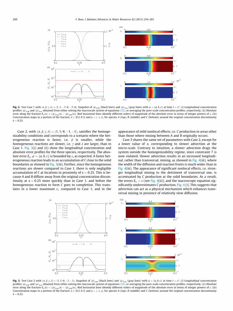
Fig. 2. Test Case 1 with ða;b; c; dÞ ¼ ð1;1;�7=4;�7=4Þ. Snapshot of hwiB;M (black lines) and hwiB;m (gray lines) with w ¼ fa; b; cg at time t ¼ ea . (i) Longitudinal concentrationprofiles hwiB;M and hwiB;m obtained from either solving the macroscale system of equations (33), or averaging the pore-scale concentration profiles, respectively. (ii) Absoluteerror along the fracture EwðxÞ ¼ jhwiB;mðxÞ � hwiB;MðxÞj. Red horizontal lines identify different orders of magnitude of the absolute error in terms of integer powers of e. (iii)Concentration maps in a portion of the fracture, x 2 ½0:2;0:3� and y ¼ ½�e; e�, for species A (top), B (middle) and C (bottom) around the original concentration discontinuity�x ¼ 0:25.

260 F. Boso, I. Battiato / Advances in Water Resources 62 (2013) 254–265

Case 2, with ða; b; c; dÞ ¼ ð1;1=4;�1;�1Þ, satisfies the homoge-nizability conditions and corresponds to a scenario where the het-erogeneous reaction is faster, i.e. b is smaller, while thehomogeneous reactions are slower, i.e. c and d are larger, than inCase 1. Fig. 3(i) and (ii) show the longitudinal concentration andabsolute error profiles for the three species, respectively. The abso-lute error Ew;w ¼ fa; b; cg is bounded by e, as expected. A faster het-erogeneous reaction leads to an accumulation of C close to the solidboundaries as showed in Fig. 3(iii). Further, since the homogeneousreactions are slower compared to Case 1, there is only negligibleaccumulation of C at locations in proximity of x ¼ 0:25. This is be-cause A and B diffuse away from the original concentration discon-tinuity at x ¼ 0:25 more quickly than in Case 1, and before thehomogeneous reaction to form C goes to completion. This trans-lates in a lower maximum ce compared to Case 1, and in the

Fig. 3. Test Case 2 with ða; b; c; dÞ ¼ ð1;1=4;�1;�1Þ. Snapshot of hwiB;M (black lines) anprofiles hwiB;M and hwiB;m obtained from either solving the macroscale system of equationerror along the fracture EwðxÞ ¼ jhwiB;mðxÞ � hwiB;MðxÞj. Red horizontal lines identify diffeConcentration maps in a portion of the fracture, x 2 ½0:2;0:3� and y ¼ ½�e; e�, for species�x ¼ 0:25.

appearance of mild nonlocal effects, i.e. C production in areas otherthan those where mixing between A and B originally occurs.

Case 3 shares the same set of parameters with Case 2, except fora lower value of a, corresponding to slower advection at themicro-scale. Contrary to intuition, a slower advection drags thesystem outside the homogenizability regime, since constraint 7 isnow violated. Slower advection results in an increased longitudi-nal, rather than transversal, mixing, as showed in Fig. 4(iii), wherethe width of the diffusion and reaction fronts is much wider than inFig. 4(iii). The appearance of significant nonlocal effects, i.e. stron-ger longitudinal mixing to the detriment of transversal one, isaccentuated by C production at the solid boundaries. As a result,the errors Ew > e (see Fig. 4(ii)), and the macroscopic equation sig-nificantly underestimates C production, Fig. 4 (i). This suggests thatadvection can act as a physical mechanism which enhances trans-versal mixing in presence of relatively slow diffusion.

d hwiB;m (gray lines) with w ¼ fa; b; cg at time t ¼ ea . (i) Longitudinal concentrations (33), or averaging the pore-scale concentration profiles, respectively. (ii) Absolute

rent orders of magnitude of the absolute error in terms of integer powers of e. (iii)A (top), B (middle) and C (bottom) around the original concentration discontinuity

Fig. 4. Test Case 3 with ða;b; c; dÞ ¼ ð1=2;1=4;�1;�1Þ. Snapshot of hwiB;M (black lines) and hwiB;m (gray lines) with w ¼ fa; b; cg at time t ¼ ea . (i) Longitudinal concentrationprofiles hwiB;M and hwiB;m obtained from either solving the macroscale system of equations (33), or averaging the pore-scale concentration profiles, respectively. (ii) Absoluteerror along the fracture EwðxÞ ¼ jhwiB;mðxÞ � hwiB;MðxÞj. Red horizontal lines identify different orders of magnitude of the absolute error in terms of integer powers of e. (iii)Concentration maps in a portion of the fracture, x 2 ½0:2;0:3� and y ¼ ½�e; e�, for species A (top), B (middle) and C (bottom) around the original concentration discontinuity�x ¼ 0:25.

F. Boso, I. Battiato / Advances in Water Resources 62 (2013) 254–265 261

An increase in the heterogeneous reaction rate compared toCase 2 leads to a reaction-driven regime at the microscale, i.e.b < 0, which drives the system outside the homogenizabilityregion (Case 4). At the pore-scale, the production of C fromdissolution of the fracture boundary dominates its productiondue to mixing of A and B (Fig. 5(iii)). Therefore, C is not concen-trated around the discontinuity front, and is poorly mixed in thetransversal direction, i.e. ceðx; yÞ � ceðyÞ. As a result, the contin-uum-scale solution hciB;M significantly overestimates the actual va-lue of the averaged pore-scale concentration hciB;m (Fig. 5(i)). Thisleads to Ec > e along the fracture, while Ea and Eb are still boundedby e, as showed in Fig. 5(ii). It is worth noticing that failed mixing

Fig. 5. Test Case 4 with ða; b; c; dÞ ¼ ð1;�1;�1;�1Þ. Snapshot of hwiB;M (black lines) andprofiles hwiB;M and hwiB;m obtained from either solving the macroscale system of equationerror along the fracture EwðxÞ ¼ jhwiB;mðxÞ � hwiB;MðxÞj. Red horizontal lines identify diffeConcentration maps in a portion of the fracture, x 2 ½0:2;0:3� and y ¼ ½�e; e�, for species�x ¼ 0:25.

at the pore-scale (i.e. in the y-direction) leads to a global break-down of the continuum-scale solution, i.e. EcðxÞ > e for any x.

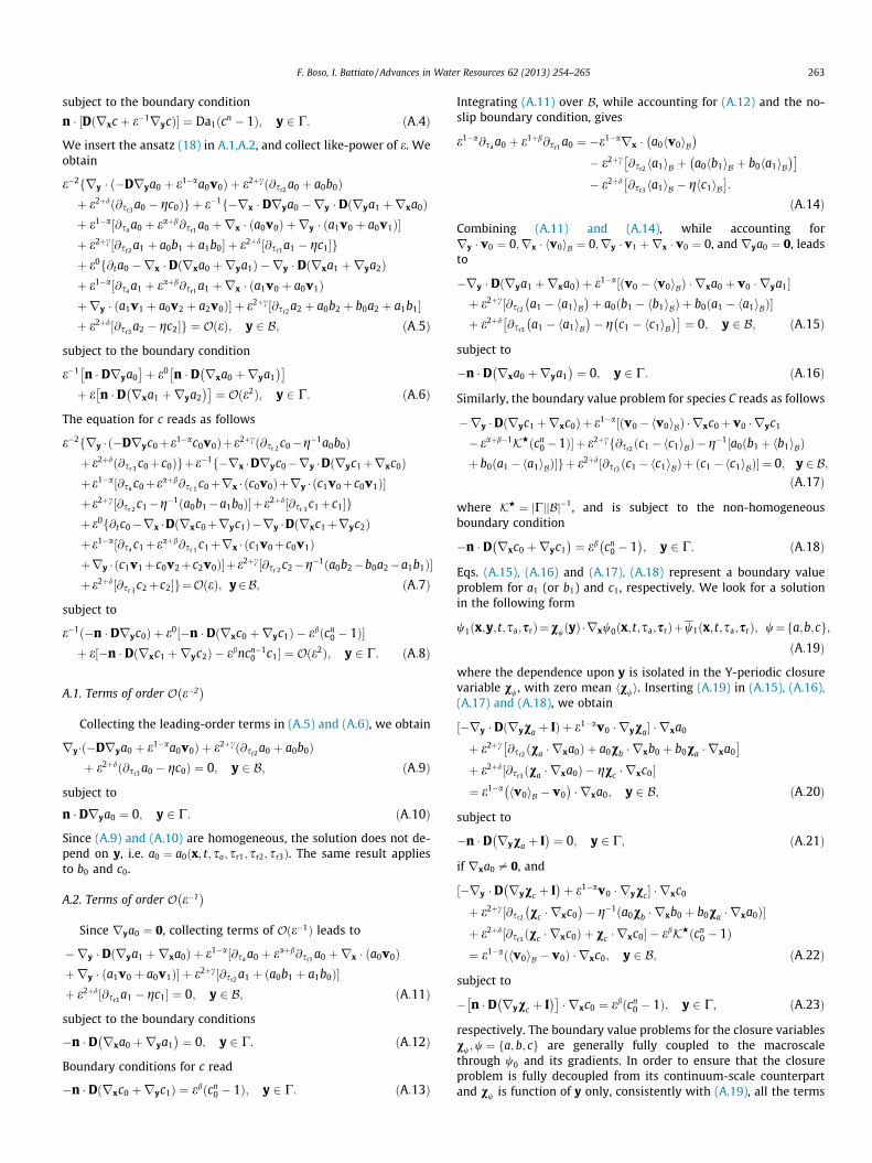
The last test case (Case 5) exhibits the same set of parameters asCase 1, except for a slower advection, i.e. smaller a. Similarly toCase 3, a slower advection drives the system outside the homoge-nizability regime, and translates into wider diffusive and reactingfronts, as showed in Fig. 6(iii). The product C diffuses longitudinallyalong the fracture much more efficiently: this leads to an averagedmicroscopic concentration hciB;m with a nearly uniform profile (seeFig. 6.(i)) along the fracture, compared to its macroscopic valuehciB;M which cannot properly capture C longitudinal diffusion afterits production due to mixing of A and B. Fig. 6(i) shows that themacroscopic equation significantly overestimates hcei, while

hwiB;m (gray lines) with w ¼ fa; b; cg at time t ¼ ea . (i) Longitudinal concentrations (33), or averaging the pore-scale concentration profiles, respectively. (ii) Absolute

rent orders of magnitude of the absolute error in terms of integer powers of e. (iii)A (top), B (middle) and C (bottom) around the original concentration discontinuity

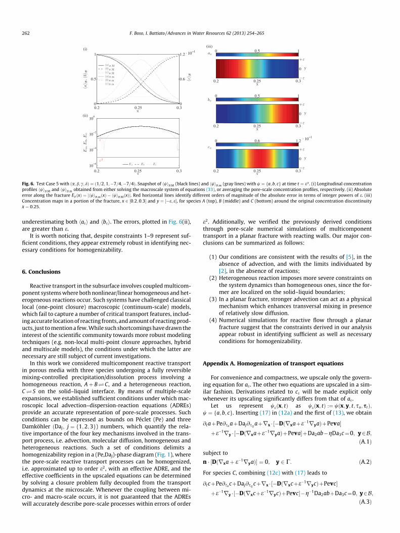
Fig. 6. Test Case 5 with ða; b; c; dÞ ¼ ð1=2;1;�7=4;�7=4Þ. Snapshot of hwiB;M (black lines) and hwiB;m (gray lines) with w ¼ fa; b; cg at time t ¼ ea . (i) Longitudinal concentrationprofiles hwiB;M and hwiB;m obtained from either solving the macroscale system of equations (33), or averaging the pore-scale concentration profiles, respectively. (ii) Absoluteerror along the fracture EwðxÞ ¼ jhwiB;mðxÞ � hwiB;MðxÞj. Red horizontal lines identify different orders of magnitude of the absolute error in terms of integer powers of e. (iii)Concentration maps in a portion of the fracture, x 2 ½0:2;0:3� and y ¼ ½�e; e�, for species A (top), B (middle) and C (bottom) around the original concentration discontinuity�x ¼ 0:25.

262 F. Boso, I. Battiato / Advances in Water Resources 62 (2013) 254–265

underestimating both haei and hbei. The errors, plotted in Fig. 6(ii),are greater than e.

It is worth noticing that, despite constraints 1–9 represent suf-ficient conditions, they appear extremely robust in identifying nec-essary conditions for homogenizability.

6. Conclusions

Reactive transport in the subsurface involves coupled multicom-ponent systems where both nonlinear/linear homogeneous and het-erogeneous reactions occur. Such systems have challenged classicallocal (one-point closure) macroscopic (continuum-scale) models,which fail to capture a number of critical transport features, includ-ing accurate location of reacting fronts, and amount of reacting prod-ucts, just to mention a few. While such shortcomings have drawn theinterest of the scientific community towards more robust modelingtechniques (e.g. non-local multi-point closure approaches, hybridand multiscale models), the conditions under which the latter arenecessary are still subject of current investigations.

In this work we considered multicomponent reactive transportin porous media with three species undergoing a fully reversiblemixing-controlled precipitation/dissolution process involving ahomogeneous reaction, Aþ B�C, and a heterogeneous reaction,C� S on the solid–liquid interface. By means of multiple-scaleexpansions, we established sufficient conditions under which mac-roscopic local advection–dispersion-reaction equations (ADREs)provide an accurate representation of pore-scale processes. Suchconditions can be expressed as bounds on Péclet (Pe) and threeDamköhler ðDaj; j ¼ f1;2;3g) numbers, which quantify the rela-tive importance of the four key mechanisms involved in the trans-port process, i.e. advection, molecular diffusion, homogeneous andheterogeneous reactions. Such a set of conditions delimits ahomogenizability region in a (Pe,Daj)-phase diagram (Fig. 1), wherethe pore-scale reactive transport processes can be homogenized,i.e. approximated up to order e2, with an effective ADRE, and theeffective coefficients in the upscaled equations can be determinedby solving a closure problem fully decoupled from the transportdynamics at the microscale. Whenever the coupling between mi-cro- and macro-scale occurs, it is not guaranteed that the ADREswill accurately describe pore-scale processes within errors of order

e2. Additionally, we verified the previously derived conditionsthrough pore-scale numerical simulations of multicomponenttransport in a planar fracture with reacting walls. Our major con-clusions can be summarized as follows:

(1) Our conditions are consistent with the results of [5], in theabsence of advection, and with the limits individuated by[2], in the absence of reactions;

(2) Heterogeneous reaction imposes more severe constraints onthe system dynamics than homogeneous ones, since the for-mer are localized on the solid–liquid boundaries;

(3) In a planar fracture, stronger advection can act as a physicalmechanism which enhances transversal mixing in presenceof relatively slow diffusion.

(4) Numerical simulations for reactive flow through a planarfracture suggest that the constraints derived in our analysisappear robust in identifying sufficient as well as necessaryconditions for homogenizability.

Appendix A. Homogenization of transport equations

For convenience and compactness, we upscale only the govern-ing equation for ae. The other two equations are upscaled in a sim-ilar fashion. Derivations related to ce will be made explicit onlywhenever its upscaling significantly differs from that of ae.

Let us represent weðx; tÞ as weðx; tÞ :¼ wðx; y; t; sa; srÞ;w ¼ fa; b; cg. Inserting (17) in (12a) and the first of (13), we obtain

@taþPe@sa aþDaj@srjaþrx � ½�Dðrxaþe�1ryaÞþPeva�

þe�1ry � ½�Dðrxaþe�1ryaÞþPeva�þDa2ab�gDa3c¼0; y2B;ðA:1Þ

subject to

n � ½Dðrxaþ e�1ryaÞ� ¼ 0; y 2 C: ðA:2Þ

For species C, combining (12c) with (17) leads to

@tcþPe@sa cþDaj@srjcþrx � ½�Dðrxcþe�1rycÞþPevc�

þe�1ry � ½�Dðrxcþe�1rycÞþPevc��g�1Da2abþDa3c¼0; y2B;ðA:3Þ

F. Boso, I. Battiato / Advances in Water Resources 62 (2013) 254–265 263

subject to the boundary condition

n � ½Dðrxc þ e�1rycÞ� ¼ Da1ðcn � 1Þ; y 2 C: ðA:4Þ

We insert the ansatz (18) in A.1,A.2, and collect like-power of e. Weobtain

e�2fry � ð�Drya0 þ e1�aa0v0Þ þ e2þcð@sr2 a0 þ a0b0Þþ e2þdð@sr3 a0 � gc0Þg þ e�1f�rx � Drya0 �ry � Dðrya1 þrxa0Þþ e1�a½@sa a0 þ eaþb@sr1 a0 þrx � ða0v0Þ þ ry � ða1v0 þ a0v1Þ�þ e2þc½@sr2 a1 þ a0b1 þ a1b0� þ e2þd½@sr3 a1 � gc1�gþ e0f@ta0 �rx � Dðrxa0 þrya1Þ � ry � Dðrxa1 þrya2Þþ e1�a½@sa a1 þ eaþb@sr1 a1 þrx � ða1v0 þ a0v1Þþ ry � ða1v1 þ a0v2 þ a2v0Þ� þ e2þc½@sr2 a2 þ a0b2 þ b0a2 þ a1b1�þ e2þd½@sr3 a2 � gc2�g ¼ OðeÞ; y 2 B; ðA:5Þ

subject to the boundary condition

e�1 n � Drya0�

þ e0 n � D rxa0 þrya1� ��

þ e n � D rxa1 þrya2� ��

¼ Oðe2Þ; y 2 C: ðA:6Þ

The equation for c reads as follows

e�2fry � ð�Dryc0þe1�ac0v0Þþe2þcð@sr 2 c0�g�1a0b0Þþe2þdð@sr 3 c0þc0Þgþe�1f�rx �Dryc0�ry �Dðryc1þrxc0Þþe1�a½@sa c0þeaþb@sr 1 c0þrx � ðc0v0Þþry � ðc1v0þc0v1Þ�þe2þc½@sr 2 c1�g�1ða0b1�a1b0Þ�þe2þd½@sr 3 c1þc1�gþe0f@tc0�rx �Dðrxc0þryc1Þ�ry �Dðrxc1þryc2Þþe1�a½@sa c1þeaþb@sr 1 c1þrx � ðc1v0þc0v1Þþry � ðc1v1þc0v2þc2v0Þ�þe2þc½@sr 2 c2�g�1ða0b2�b0a2�a1b1Þ�þe2þd½@sr 3 c2þc2�g¼OðeÞ; y2B; ðA:7Þ

subject to

e�1ð�n � Dryc0Þ þ e0½�n � Dðrxc0 þryc1Þ � ebðcn0 � 1Þ�

þ e½�n � Dðrxc1 þryc2Þ � ebncn�10 c1� ¼ Oðe2Þ; y 2 C: ðA:8Þ

A.1. Terms of order O e�2� �

Collecting the leading-order terms in (A.5) and (A.6), we obtain

ry�ð�Drya0 þ e1�aa0v0Þ þ e2þcð@sr2 a0 þ a0b0Þþ e2þdð@sr3 a0 � gc0Þ ¼ 0; y 2 B; ðA:9Þ

subject to

n � Drya0 ¼ 0; y 2 C: ðA:10Þ

Since (A.9) and (A.10) are homogeneous, the solution does not de-pend on y, i.e. a0 ¼ a0 x; t; sa; sr1; sr2; sr3ð Þ. The same result appliesto b0 and c0.

A.2. Terms of order O e�1� �

Since rya0 ¼ 0, collecting terms of Oðe�1Þ leads to

�ry � Dðrya1 þrxa0Þ þ e1�a½@sa a0 þ eaþb@sr1 a0 þrx � ða0v0Þþ ry � ða1v0 þ a0v1Þ� þ e2þc½@sr2 a1 þ ða0b1 þ a1b0Þ�þ e2þd½@sr3 a1 � gc1� ¼ 0; y 2 B; ðA:11Þ

subject to the boundary conditions

�n � D rxa0 þrya1� �

¼ 0; y 2 C: ðA:12Þ

Boundary conditions for c read

�n � Dðrxc0 þryc1Þ ¼ ebðcn0 � 1Þ; y 2 C: ðA:13Þ

Integrating (A.11) over B, while accounting for (A.12) and the no-slip boundary condition, gives

e1�a@sa a0 þ e1þb@sr1 a0 ¼ �e1�arx � a0 v0h iB� �

� e2þc @sr2 a1h iB þ a0 b1h iB þ b0 a1h iB� ��

� e2þd @sr3 a1h iB � g c1h iB�

:

ðA:14Þ

Combining (A.11) and (A.14), while accounting forry � v0 ¼ 0;rx � v0h iB ¼ 0;ry � v1 þrx � v0 ¼ 0, and rya0 ¼ 0, leadsto

�ry � Dðrya1 þrxa0Þ þ e1�a½ðv0 � v0h iBÞ � rxa0 þ v0 � rya1�þ e2þc½@sr2 a1 � a1h iB

� �þ a0ðb1 � b1h iBÞ þ b0ða1 � a1h iBÞ�

þ e2þd @sr3 a1 � a1h iB� �

� g c1 � c1h iB� ��

¼ 0; y 2 B; ðA:15Þ

subject to

�n � D rxa0 þrya1� �

¼ 0; y 2 C: ðA:16Þ

Similarly, the boundary value problem for species C reads as follows

�ry �Dðryc1 þrxc0Þ þ e1�a½ðv0 � v0h iBÞ �rxc0 þv0 � ryc1

� eaþb�1KHðcn0 � 1Þ� þ e2þcf@sr2 ðc1 � c1h iBÞ � g�1½a0ðb1 þ b1h iBÞ

þ b0ða1 � a1h iBÞ�gþ e2þd½@sr3 ðc1 � c1h iBÞ þ ðc1 � c1h iBÞ� ¼ 0; y 2 B;ðA:17Þ

where KH ¼ Cj j Bj j�1, and is subject to the non-homogeneousboundary condition

�n � D rxc0 þryc1� �

¼ eb cn0 � 1

� �; y 2 C: ðA:18Þ

Eqs. (A.15), (A.16) and (A.17), (A.18) represent a boundary valueproblem for a1 (or b1) and c1, respectively. We look for a solutionin the following form

w1ðx;y;t;sa;srÞ¼vw yð Þ �rxw0ðx;t;sa;srÞþw1ðx;t;sa;srÞ; w¼fa;b;cg;ðA:19Þ

where the dependence upon y is isolated in the Y-periodic closurevariable vw, with zero mean hvwi. Inserting (A.19) in (A.15), (A.16),(A.17) and (A.18), we obtain

½�ry � Dðryva þ IÞ þ e1�av0 � ryva� � rxa0

þ e2þc @sr2 ðva � rxa0Þ þ a0vb � rxb0 þ b0va � rxa0�

þ e2þd½@sr3 ðva � rxa0Þ � gvc � rxc0�¼ e1�a v0h iB � v0

� �� rxa0; y 2 B; ðA:20Þ

subject to

�n � D ryva þ I� �

¼ 0; y 2 C; ðA:21Þ

if rxa0 – 0, and

½�ry � D ryvc þ I� �

þ e1�av0 � ryvc� � rxc0

þ e2þc½@sr2 vc � rxc0� �

� g�1ða0vb � rxb0 þ b0va � rxa0Þ�þ e2þd½@sr3 ðvc � rxc0Þ þ vc � rxc0� � ebKHðcn

0 � 1Þ¼ e1�aðhv0iB � v0Þ � rxc0; y 2 B; ðA:22Þ

subject to

� n � D ryvc þ I� ��

� rxc0 ¼ ebðcn0 � 1Þ; y 2 C; ðA:23Þ

respectively. The boundary value problems for the closure variablesvw;w ¼ fa; b; cg are generally fully coupled to the macroscalethrough w0 and its gradients. In order to ensure that the closureproblem is fully decoupled from its continuum-scale counterpartand vw is function of y only, consistently with (A.19), all the terms

264 F. Boso, I. Battiato / Advances in Water Resources 62 (2013) 254–265

in (A.20)–(A.23) containing macroscopic quantities must be negligi-ble as e� 1. We first observe that no additional constraints are re-quired to decouple (A.20)-(A.21) from the macroscale problem, if vc

is function of y only. We start with the boundary value problem(A.22)-(A.23) for vc . The right-hand side in (A.23) is negligible com-pared to the left-hand side if b > 0 (constraint 4). Additionally, forthe terms of order eb; e2þc and e2þd to be negligible relative to thesmallest term in (A.22), b; c and d must satisfy the followingconstraints: b > maxf0;1� ag;2þ c > maxf0;1� ag, and2þ d > maxf0;1� ag, respectively. Since a < 2 (constraint 3), thenb > 0; c > �2 (constraint 5) and d > �2 (constraint 6) if 1 < a < 2,and b > 1� a (constraint 7), c > �1� a (constraint 8) andd > �1� a (constraint 9) if a < 1.

A.3. Terms of order O e0� �

Collecting terms of order e0 in (A.5), leads to

@ta0 �rx � Dðrxa0 þrya1Þ � ry � Dðrxa1 þrya2Þþ e1�a½@sa a1 þ eaþb@sr1 a1 þrx � ða1v0 þ a0v1Þþ ry � ða1v1 þ a0v2 þ a2v0Þ� þ e2þc½@sr2 a2 þ a0b2 þ b0a2 þ a1b1�þ e2þd½@sr3 a2 � gc2� ¼ 0; y 2 B; ðA:24Þ

subject to

�n � Dðrxa1 þrya2Þ ¼ 0; y 2 C: ðA:25Þ

Integration of (A.24) over B with respect to y while accounting for(A.25), (A.19) and periodicity, leads to

@tha0iB � rx � hDðIþryvaÞiBrxa0

þ e1�a½@saha1iB þ eaþb@sr1 ha1iB þ rx � ðha1v0iB þ a0hv1iBÞ�þ e2þc½@sr2 ha2iB þ a0hb2iB þ b0ha2iB þ ha1b1iB�þ e2þd½@sr3 ha2iB � ghc2iB� ¼ 0: ðA:26Þ

We insert (A.19) in (A.26) while accounting for the relationshipsw0 ¼ hw0iB and v0 ¼ �kðyÞ � rxp0, and obtain

@tha0iB þ e1�a@sa ha1iB þ e1þb@sr1 ha1iB þ e2þc@sr2 ha2iBþ e2þd@sr3 ha2iB ¼ rx � ð/�1DHrxha0iBÞ� /�1e1�arx � ðha0iBhv1i þ �a1hv0iÞ � e2þcðha0iBhb2iBþ hb0iBha2iB þ ha1b1iBÞ þ e2þdghc2iB; ðA:27Þ

where DH ¼ hDðIþryvaÞi þ e1�ahvakirxp0. Multiplying (A.27) by eand adding it to (A.14) and to the integral of (A.9) over B gives

e@thaiB ¼ erx � ð/�1DHrxha0iBÞ � e1�arx � ðha0iBhv0iBþ eha0iBhv1iB þ e�a1hv0iBÞ � e1þc½ha0iBhb0iBþ eðha0iBhb1iB þ hb0iBha1iBÞ þ e2ðha0iBhb2iBþ hb0iBha2iB þ ha1b1iBÞ� þ e1þdgðhc0iB þ ehc1iBþ e2 c2h iBÞ þ Oðe2Þ; ðA:28Þ

since hwiB ¼ hweiB ¼ hw0iB þ ehw1iB þ Oðe2Þ, and

e@thaiB ¼ e@tha0iB þ e1�a@sa ha0iB þ eDaj@srjha0iB þ eðe@tha1iB

þ e1�a@sa ha1iB þ eDaj@srjha1iBÞ þ Oðe2Þ ðA:29Þ

with Daj, j ¼ f1;2;3g, defined in (19). Additionally, using (A.19), (18)and (15), it can be showed that �a1 ¼ ha1iB; haiBhviB ¼ ha0iBhv0iBþeha0iBhv1iB + eha1iBhv0iB þ Oðe2Þ; ehaiB ¼ eha0iB þ Oðe2Þ andhaiBhbiB ¼ ha0iBhb0iB þ eðha0iBhb1iB þ hb0iBha1iBÞ þ Oðe2Þ. Finally,accounting for the previous equalities while retaining terms of orderup to e in (A.28), we obtain (22a). The latter describes pore-scale pro-cesses within errors of order e2.

Collecting terms of order e0 in (A.7) leads to

@tc0 �rx � Dðrxc0 þryc1Þ � ry � Dðrxc1 þryc2Þþ e1�a½@sa c1 þ eaþb@sr1 c1 þrx � ðc1v0 þ c0v1Þþ ry � ðc1v1 þ c0v2 þ c2v0Þ�þ e2þc½@sr2 c2 � g�1ða0b2 þ b0a2 þ a1b1Þ�þ e2þd½@sr3 c2 þ c2� ¼ 0; y 2 B; ðA:30Þ

subject to

�n � Dðrxc1 þryc2Þ ¼ nebcn�10 c1; y 2 C: ðA:31Þ

A similar procedure to that just presented allows one to derive (22c)for hciB ¼ hc0iB þ ehc1iB þ Oðe2Þ, while imposing the additional con-straint hvciC ¼ hvciB . Eqs. (22a)–(22c) govern the dynamics ofhaiB; hbiB and hciB up to e2.

Appendix B. Notation

ae dimensionless pore-scale aqueous concentration of species A.ae pore-scale aqueous concentration of species A, [mol L�3].

haei average of ae over the unit cell Y.

haeiB average of ae over the pore volume B.

haeiC average of ae over the solid–liquid interface C.be dimensionless aqueous concentration of species B.be pore-scale aqueous concentration of species B, [mol L�3].

hbei average of be over the unit cell Y.

hbeiB average of be over the pore volume B.

hbeiC average of be over the solid–liquid interface C.B pore space domain in the unit cell Y.jBj volume of B.Be pore space domain in the porous medium X.ce dimensionless pore-scale aqueous concentration of species C.ce pore-scale aqueous concentration of species C, [mol L�3].

hcei average of ce over the unit cell Y.

hceiB average of ce over the pore volume B.

hceiC average of ce over the solid–liquid interface C.

c :¼ffiffiffiffiffiffiffiffiffiffikd=kn

p, threshold aqueous concentration of species C, [mol

L�3].cH :¼maxfain; bing, characteristic value of concentrations a and

b, [mol L�3].D dimensionless molecular diffusion coefficient defined by (7).D :¼ Da ¼ Db ¼ Dc , [L2T�1].Di i ¼ fa; b; cg, molecular diffusion coefficients for species A;B

and C, respectively, [L2T�1].D0 characteristic value of D, [L2T�1].DH dimensionless dispersion tensor defined by (23).

Daj :¼ td=trj; j ¼ f1;2;3g, Damköhler numbers defined by (9).G solid matrix domain in the unit cell Y.k reaction rate of the forward heterogeneous reaction C ! S.

kab reaction rate of the forward homogeneous reactionAþ B! C.

kc reaction rate of the backward homogeneous reactionAþ B C.

kd reaction rate of the backward heterogeneous reaction C S.k closure variable defined by (21).K :¼ hkðyÞi, permeability tensor.KH effective reaction rate constant defined by (23).‘ characteristic length of the periodic unit cell Y .L characteristic length of macroscopic porous medium domain

X.n heterogeneous reaction order, [-].p fluid dynamic pressure, [ML�1T�2].

Pe Péclet number defined by (9).Rp :¼ kcn

e , precipitation rate.

F. Boso, I. Battiato / Advances in Water Resources 62 (2013) 254–265 265

Rd :¼ kd, dissolution rate.t :¼ t=td, dimensionless time.

ta advection timescale, [T].td diffusion timescale, [T].trj j ¼ f1;2;3g, reaction timescales, [T].U characteristic velocity associated to ve, [TL�1].ve dimensionless pore-scale fluid velocity.ve pore-scale fluid velocity, [TL�1].x spatial coordinate of the pore space Be.y spatial coordinate of the unit cell Y.Y spatially periodic unit cell.jY j volume of the spatially periodic unit cell.e :¼ ‘=L, scale separation coefficient, [-].g :¼ c=cH, normalization coefficient, [-]./ unit cell porosity, [-].C solid–liquid interface in the unit cell Y.Ce solid–liquid interface in the porous medium X.m fluid dynamic viscosity, [ML�1T�1].

vw w ¼ fa; b; cg, closure variable for the transport problem ofspecies w.

X porous medium domain.win w ¼ fa; b; cg, initial dimensionless concentration for species w.

References

[1] Allaire G, Brizzi R, Mikelic A, Piatnitski A. Two-scale expansion with driftapproach to the Taylor dispersion for reactive transport through porous media.Chem Eng Sci 2010;65:2292–300.

[2] Auriault JL, Adler PM. Taylor dispersion in porous media: analysis by multiplescale expansions. Adv Water Resour 1995;18(4):217–26.

[3] Battiato I. Self-similarity in coupled Brinkman/Navier–Stokes flows. J FluidMech 2012;699:94–114.

[4] Battiato I, Bandaru PR, Tartakovsky DM. Elastic response of carbon nanotubeforests to aerodynamic stresses. Phys Rev Lett 2010;105(14):144504.

[5] Battiato I, Tartakovsky DM. Applicability regimes for macroscopic models ofreactive transport in porous media. J Contam Hydrol 2011;120–121:18–26.

[6] Battiato I, Tartakovsky DM, Tartakovsky AM, Scheibe TD. On breakdown ofmacroscopic models of mixing-controlled heterogeneous reactions in porousmedia. Adv Water Resour 2009;32:1664–73.

[7] Battiato I, Tartakovsky DM, Tartakovsky AM, Scheibe TM. Hybrid models ofreactive transport in porous and fractured media. Adv Water Resour2011;34(9):1140–50.

[8] Bear J. Dynamics of fluids in porous media. Dover; 1988.[9] Blunt MJ, Jackson MD, Piri M, Valvatne PH. Detailed physics, predictive

capabilities and macroscopic consequences for pore-network models ofmultiphase flow. Adv Water Resour 2002;25:1069–89.

[10] Boso F, Bellin A, Dumbser M. Numerical simulations of solute transport inhighly heterogeneous formations: A comparison of alternative numericalschemes. Adv Water Resour 2013;52:178–89.

[11] Brenner H. Transport processes in porous media. McGraw-Hill; 1987.[12] Choi T-J, Maurya MR, Tartakovsky DM, Subramaniam S. Stochastic hybrid

modeling of intracellular calcium dynamics. J Chem Phys2010;133(16):166101.

[13] Darcy H. Les fontaines publiques de la ville de Dijon. Paris: Victor Dalmont;1856.

[14] Dentz M, Borgne TL, Englert A, Bijeljic B. Mixing spreading and reaction inheterogeneous media: a brief review. J Contam Hydrol 2011;120–121(0):1–17.

[15] Golfier F, Wood BD, Orgogozo L, Quintard M, Buès M. Biofilms in porous media:development of macroscopic transport equations via volume averaging withclosure for local mass equilibrium conditions. Adv Water Resour2009;32(3):463–85.

[16] Gray WG, Miller CT. Thermodynamically constrained averaging theoryapproach for modeling flow and transport phenomena in porous mediumsystems: 7. single-phase megascale flow models. Adv Water Resour2009;32(8):1121–42.

[17] Herrera PA, Massabó M, Beckie RD. A meshless method to simulate solutetransport in heterogeneous porous media. Adv Water Resour2009;32(3):413–29.

[18] Higgins ER, Goel P, Puglisi JL, Bers DM, Cannell M, Sneyd J. Modelling calciummicrodomains using homogenisation. J Theor Biol 2007;247(4):623–44.

[19] Hornung U. Homogenization and porous media. New York: Springer; 1997.[20] Knabner P, Duijn CJV, Hengst S. An analysis of crystal dissolution fronts in

flows through porous media. Part 1: compatible boundary conditions. AdvWater Resour 1995;18(3):171–85.

[21] Li L, Steefel CI, Yang L. Scale dependence of mineral dissolution rates withinsingle pores and fractures. Geochim Cosmochim Ac 2008;72(2):360–77.

[22] Meile C, Tuncay K. Scale dependence of reaction rates in porous media. AdvWater Resour 2006;29:62–71.

[23] Mikelic A, Devigne V, Van Duijn CJ. Rigorous upscaling of the reactive flowthrough a pore, under dominant Péclet and Damköhler numbers. SIAM J MathAnal 2006;38(4):1262–87.

[24] Molins S, Trebotich D, Steefel CI, Shen CP, An investigation of the effect of porescale flow on average geochemical reaction rates using direct numericalsimulation, Water Resour Res, vol. 48 (W03527).

[25] Morse JW, Arvidson RS. The dissolution kinetics of major sedimentarycarbonate minerals. Earth Sci Rev 2002;58:51–84.

[26] Neuman SP, Tartakovsky DM. Perspective on theories of anomalous transportin heterogeneous media. Adv Water Resour 2009;32(5):670–80.

[27] Pacala S, Socolow R. Stabilization wedges: solving the climate problem for thenext 50 years with current technologies. Science 2004;305(5686):968–72.

[28] Peter MA. Analysis homogenization coupled reaction–diffusion processesinducing an evolution of the microstructure: analysis and homogenization.Nonlinear Anal : Theory Methods Appl 2009;70(2):806–21.

[29] Tartakovsky AM, Meakin P, Scheibe T. Simulations of reactive transport andprecipitation with smoothed particle hydrodynamics. J Comput Phys2007;222(2):654–72.

[30] Tartakovsky AM, Redden G, Lichtner PC, Scheibe TD, Meakin P. Mixing-inducedprecipitation: experimental study and multi-scale numerical analysis. WaterResour Res 2008;44(W06S04):19.

[31] Tartakovsky AM, Tartakovsky DM, Scheibe TD, Meakin P. Hybrid simulations ofreaction–diffusion systems in porous media. SIAM J Sci Comput2007;30(6):2799–816.

[32] Tartakovsky AM, Tartakovsky GD, Scheibe TD. Effects of incomplete mixing onmulticomponent reactive transport. Adv Water Resour 2009;32(11):1674–9.

[33] Van Leemput P, Vandekerckhove C, Vanroose W, Roose D. Accuracy of hybridlattice boltzmann/finite difference schemes for reaction-diffusion systems.Multiscale Model Simul 2007;6(3):838–57.

[34] van Noorden TL, Pop IS. A Stefan problem modelling crystal dissolution andprecipitation. IMA J Appl Math 2008;73(2):393–411.

[35] Whitaker S. Levels of simplification: the use of assumptions, restrictions, andconstraints in engineering analysis. Chem Eng Educ 1988;22:104–8.

[36] Whitaker S. The method of volume averaging. Kluwer Academic Publishers.;1999.

[37] Willingham TW, Werth CJ, Valocchi AJ. Evaluation of the effects of porousmedia structure on mixing-controlled reactions using pore-scale modeling andmicromodel experiments. Environ Sci Technol 2008;42(9):3185–93.

[38] Wood BD, Radakovich K, Golfier F. Effective reaction at a fluid-solid interface:applications to biotransformation in porous media. Adv Water Resour2007;30:1630–47.