Data 100, Summer 2021

Homework #6

Total Points: 26

Submission Instructions

You must submit this assignment to Gradescope by Monday, July 19th, at 11:59PM. While Gradescope accepts late submissions, you will not receive any credit for a latesubmission if you do not have prior accommodations (e.g. DSP).

You can work on this assignment in any way you like.

• One way is to download this PDF, print it out, and write directly on these pages (we’veprovided enough space for you to do so). Alternatively, if you have a tablet, you couldsave this PDF and write directly on it.

• Another way is to use some form of LaTeX. Overleaf is a great tool.

• You could also write your answers on a blank sheet of paper.

Regardless of what method you choose, the end result needs to end up on Gradescope,as a PDF. If you wrote something on physical paper (like options 1 and 3 above), you willneed to use a scanning application (e.g. CamScanner) in order to submit your work.

When submitting on Gradescope, you must assign pages to each question correctly (itprompts you to do this after submitting your work). This significantly streamlines thegrading process for our tutors. Failure to do this may result in a score of 0 for any questionsthat you didn’t correctly assign pages to. If you have any questions about the submissionprocess, please don’t hesitate to ask on Piazza.

Collaborators

Data science is a collaborative activity. While you may talk with others about the home-work, we ask that you write your solutions individually. If you do discuss the assignmentswith others please include their names at the top of your submission.

1

Homework #6 2

Properties of Simple Linear Regression1. (7 points) In Lecture 12, we spent a great deal of time talking about simple linear

regression, which you also saw in Data 8. To briefly summarize, the simple linear re-gression model assumes that given a single observation x, our predicted response for thisobservation is y = θ0 + θ1x.

In Lecture 12, we saw that the θ0 and θ1 that minimize the average L2 loss for the simplelinear regression model are:

θ0 = y − θ1x

θ1 = rσyσx

Or, rearranging terms, our predictions y are:

y = y + rσyx− xσx

(a) (3 points) As we saw in lecture, a residual ei is defined to be the difference betweena true response yi and predicted response yi. Specifically, ei = yi − yi. Note thatthere are n data points, and each data point is denoted by (xi, yi).

Prove, using the equation for y above, that∑n

i=1 ei = 0.

(b) (2 points) Using your result from part a, prove that y = ¯y.

(c) (2 points) Prove that (x, y) is on the simple linear regression line.

Homework #6 3

Geometric Perspective of Least Squares

2. (7 points) In Lecture 13, we viewed both the simple linear regression model and themultiple linear regression model through the lens of linear algebra. The key geometricinsight was that if we train a model on some design matrix X and true response vectorY, our predicted response Y = Xθ is the vector in span(X) that is closest to Y.

In the simple linear regression case, our optimal vector θ is θ = [θ0, θ1]T , and our design

matrix is

X =

1 x11 x2...

...1 xn

=

| |1 ~x| |

This means we can write our predicted response vector as Y = X[θ0θ1

], and also as

Y = θ01 + θ1~x.

Note, in this problem, ~x refers to the n-length vector [x1, x2, ..., xn]T . In other words, itis a feature, not an observation.

For this problem, assume we are working with the simple linear regression model, thoughthe properties we establish here hold for any linear regression model that contains anintercept term.

(a) (3 points) Using the geometric properties from lecture, prove that∑n

i=1 ei = 0.

Hint: Recall, we define the residual vector as e = Y− Y, and e = [e1, e2, ..., en]T .

Homework #6 4

(b) (2 points) Explain why the vector ~x (as defined in the problem) and the residualvector e are orthogonal. Hint: Two vectors are orthogonal if their dot product is 0.

(c) (2 points) Explain why the predicted response vector Y and the residual vector eare orthogonal.

Homework #6 5

Properties of a Linear Model With No Constant Term

Suppose that we don’t include an intercept term in our model. That is, our model is nowsimply y = γx, where γ is the single parameter for our model that we need to optimize.(In this equation, x is a scalar, corresponding to a single observation.)

As usual, we are looking to find the value γ that minimizes the average squared loss(“empirical risk”) across our observed data {(xi, yi)}, i = 1, . . . , n.

R(γ) =1

n

n∑i=1

(yi − γxi)2

The normal equations derived in lecture no longer hold. In this problem, we’ll derive asolution to this simpler model. We’ll see that the least squares estimate of the slope inthis model differs from the simple linear regression model, and will also explore whetheror not our properties from the previous problem still hold.

3. (4 points) Use calculus to find the minimizing γ. That is, prove that

γ =

∑xiyi∑x2i

Note: This is the slope of our regression line, analogous to θ1 from our simple linearregression model.

Homework #6 6

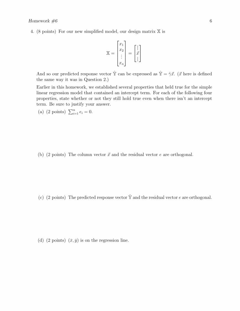
4. (8 points) For our new simplified model, our design matrix X is

X =

x1x2...xn

=

|~x|

And so our predicted response vector Y can be expressed as Y = γ~x. (~x here is definedthe same way it was in Question 2.)

Earlier in this homework, we established several properties that held true for the simplelinear regression model that contained an intercept term. For each of the following fourproperties, state whether or not they still hold true even when there isn’t an interceptterm. Be sure to justify your answer.

(a) (2 points)∑n

i=1 ei = 0.

(b) (2 points) The column vector ~x and the residual vector e are orthogonal.

(c) (2 points) The predicted response vector Y and the residual vector e are orthogonal.

(d) (2 points) (x, y) is on the regression line.

Homework #6 7

MSE “Minimizer”

5. (10 points) Recall from calculus that given some function g(x), the x you get from

solving dg(x)dx

= 0 is called a critical point of g – this means it could be a minimizer or amaximizer for g. In this question, we will explore some basic properties and build someintuition on why, for certain loss functions such as the MSE loss, the critical point ofthe loss will always be the minimizer of the loss.

Given some linear model f(x) = γx for some real scalar γ, we can write the the meansquared error (MSE) loss of the model f given the observed data {xi, yi}, i = 1, . . . , n as

1

n

n∑i=1

(yi − γxi)2.

(a) (1 point) Let’s break the loss function above into individual terms. Complete thefollowing sentence by filling in the blanks using one of the options in the parenthesisfollowing each of the blanks:

The MSE loss function can be viewed as a sum of n (linear/quadratic/log-arithmic/exponential) terms, each of which can be treated as a function of(xi/yi/γ).

(b) (3 points) Let’s investigate one of the n functions in the summation in the MSEloss function. Define gi(γ) = 1

n(yi−γxi)2 for i = 1, . . . , n. Recall from calculus that

we can use the 2nd derivative of a function to describe its curvature about a certainpoint (if it is facing concave up, down, or possibly a point of inflection). You cantake the following as a fact: A function is convex if and only if the function’s 2ndderivative is non-negative on its domain. Based on this property, verify that gi is aconvex function.

(c) (2 points) Briefly explain intuitively in words why given a convex function g(x),

the critical points we get by solving dg(x)dx

= 0 minimizes g. You can assume thatdg(x)dx

is a function of x (and not a constant).

(d) (3 points) Now that we have shown that each term in the summation of MSE isa convex function, one might wonder if the entire summation is convex given it’sa sum of convex functions. While the answer to this for a multivariable functionis out of scope for this course, we can still build some intuitions by focusing onsingle-variable functions.

i. (2 points) Let’s look at the formal definition of convex functions.Algebraically speaking, a function g(x) is convex if for any two points (x1, g(x1))and (x2, g(x2)) on the function:

g(cx1 + (1− c)x2) ≤ cg(x1) + (1− c)g(x2)

Homework #6 8

for any real constant 0 ≤ c ≤ 1.Intuitively, the above definition says that, given the plot of a convex functiong(x), if you connect 2 randomly chosen points on the function, the line segmentwill always lie on or above g(x) (try this with the graph of y = x2).Using this definition, show that if g(x) and h(x) are both convex functions,their sum g(x) + h(x) will also be a convex function.

ii. (1 point) Based on what you have shown in the previous part, explain intu-itively why the sum of n convex functions is still a convex function when n > 2.

(e) (1 point) Finally, explain why in our case that, when we solve for the critical pointof the MSE loss function by taking the gradient with respect to the parameter andsetting the expression to 0, it is guranteed that the solution we find will minimizethe MSE loss.