home/ludmila/three layer …
TRANSCRIPT
Dispersion of elastic waves in a strongly inhomogeneous
three-layered plate
J. Kaplunov∗, D.A. Prikazchikov, L.A. Prikazchikova
School of Computing and Mathematics, Keele University
Keele, Staffordshire, ST5 5BG, UK
Abstract
Elastic wave propagation in a three-layered plate with high-contrast mechanical
and geometric properties of the layers is analysed. Four specific types of contrast
arising in engineering practice, including the design of stiff and lightweight struc-
tures, laminated glass, photovoltaic panels, and electrostatic precipitators in gas
filters, are considered. For all of them the cut-off frequency of the first harmonic is
close to zero. Two-mode asymptotic polynomial expansions of the Rayleigh-Lamb
dispersion relation approximating both the fundamental bending wave and the first
harmonic, are derived. It is established that these can be either uniform or com-
posite ones, valid only over non-overlapping vicinities of zero and the lowest cut-off
frequencies. The partial differential equations of motion associated with two-mode
shortened dispersion relations are also presented.
Keywords: Vibration, sandwich plate, asymptotic, contrast.
1. Introduction
Multi-layered engineering structures, in particular three-layered symmetric plates
and shells, also known as sandwich structures, have been manufactured since long
ago. Sandwich structures, due to their light weight combined with relatively large
flexural stiffness, are in a great demand for modern aerospace, automotive, and civil5
engineering, e.g. see Vinson (1999) and references therein.
Recent technological developments intensively exploit structures with high con-
trast in material and geometrical properties of the layers, including, for example,
laminated glass beams and plates widely used in glazing and photovoltaic applica-
tions. Laminated glass is usually designed as a three-layered plate, with two stiff10
∗Corresponding authorEmail addresses: [email protected] (J. Kaplunov), [email protected]
(D.A. Prikazchikov), [email protected] (L.A. Prikazchikova)
Preprint submitted to International Journal of Solids and Structures February 1, 2017
brought to you by COREView metadata, citation and similar papers at core.ac.uk
provided by Keele Research Repository
facings and a soft polymeric interlayer, see Schulze et al. (2012) and Asık & Tezcan
(2005). For photovoltaic panels, the ratio of the shear moduli of a glass skin and
polymeric layer encapsulating solar cells, is within the range 10−5 ∼ 10−2, depend-
ing on temperature and polymer type, see Schulze et al. (2012), Altenbach et al.
(2015), Aßmus et al. (2016), Aßmus et al. (2017), and Naumenko & Eremeyev (2014).15
In automotive and civil engineering, laminated glass has a rather thin polymeric core
layer with relatively thick glass facings, resulting in a substantial contrast of core
and skin layer thicknesses. Another advanced application of multi-layered struc-
tures with high-contrast material properties is connected with the rapidly growing
area of meta-materials, e.g. see Martin et al. (2012).20
All of the aforementioned structures are characterised by stiff facings. However,
there are also important examples of structures with soft facings and a stiff core
layer. In particular, this is a feature of dust-covered precipitator plates, which are
important parts of gas filters reducing air pollution Lee & Chang (1979).
Mechanics of layered media, including sandwich structures, without a special25
emphasis on high contrast problems, has been thoroughly investigated, e.g. see
the textbooks Qatu (2004), Wang et al. (2000), Reddy (2004), and Milton (2002)
to name a few. Numerous publications deal with sandwich plates and beams, e.g.
see review articles Hohe & Librescu (2004), Kreja (2011), and Carrera & Brischetto
(2009).30
At the same time only a few considerations are oriented towards strongly inho-
mogeneous multi-layered structures. Among them, we mention asymptotic develop-
ments on the subject reported in Berdichevsky (2010), Kudaibergenov et al. (2016),
Tovstik & Tovstik (2016), and Kaplunov et al. (2016), along with Altenbach et al.
(2015) and Naumenko & Eremeyev (2014) using ad hoc layerwise theories, and35
Chapman (2013) developing finite-product approximations to the exact Rayleigh-
Lamb dispersion relation for a three-layered plate. In addition, we cite Cherdantsev & Cherednichenko
(2012), Smyshlyaev (2009), Figotin & Kuchment (1998), and Kaplunov & Nobili
(2016) devoted to homogenization of high-contrast periodic composites. Similarity
of the asymptotic procedures underlying multi-layered plate theories and homoge-40
nization for periodic media has been recently reported in Craster et al. (2014).
In this paper we present results of the asymptotic analysis of the exact dispersion
relation corresponding to plane anti-symmetric waves propagating in a three-layered
elastic plate. The main focus is on the set of problem parameters, for which the
lowest thickness shear resonance frequency tends to zero at a high-contrast limit,45
see Kaplunov et al. (2016) dealing with the identical 1D problem for an elastic
2
rod, and also Lee & Chang (1979) and Ryazantseva & Antonov (2012) studying a
sandwich plate. This cut-off frequency seemingly determines the upper bound of
the frequency domain, in which the asymptotic formulation in Berdichevsky (2010)
initially oriented to statics, is applicable.50
Four specific setups are studied, including stiff skin layers and light core layer,
stiff thin skin layers and light core layer, stiff skin layers and thin light core layer,
soft thin skin layers and light core layer. Shortened polynomial dispersion relations,
governing long-wave low-frequency behaviour, e.g. see Kaplunov et al. (1998), are
derived. All of them approximate both the fundamental and the lowest shear vibra-55
tion modes. It is remarkable that the obtained asymptotic expansions are uniformly
valid only for plates with stiff skin layers and light core layer, and stiff skin layers
and thin light core layer. Other setups allow only the so-called ’composite’ ex-
pansions, e.g. see Van Dyke (1975) and Andrianov et al. (2013), valid only over
non-overlapping vicinities of zero and the lowest thickness resonance frequencies.60
The accuracy of the established two-mode approximations is tested by numeri-
cal comparisons with the solutions of the Rayleigh-Lamb dispersion relation. The
ranges of applicability of the local one-mode approximations valid near zero and
the lowest shear thickness resonance frequencies, are also evaluated. In addition,
we present numerical data for cross-thickness variations of plate displacements.65
Finally, we restore partial differential equations of motion starting from the
established two-mode dispersion relations. This finding is preceded by preliminary
remarks emphasising an important correspondence between shortened polynomial
dispersion relations and long-wave plate theories.
2. Preliminary remarks70
Consider first an isotropic layer of thickness 2h and infinite lateral extent. With-
out loss of generality restrict ourselves to plane antisymmetric motion. In this case
the Rayleigh-Lamb dispersion relation for a layer with traction-free faces takes the
form, e.g. see Graff (2012),
γ4 sinhα
αcoshβ − β2K2 coshα
sinhβ
β= 0, (1)
with
α2 = K2 − κ2Ω2, β2 = K2 − Ω2, γ2 = K2 − 1
2Ω2. (2)
In the above
K = kh, Ω =ωh
c2, κ =
c2c1
. (3)
3
Here ω is the angular frequency, k is the wave number, c1 and c2 are the longitudinal
and shear wave speeds, respectively, given by
c21 =λ+ 2µ
ρ, c22 =
µ
ρ, (4)
where λ and µ are the Lame constants, and ρ is volume mass density.
The transcendental dispersion relation (1) allows polynomial asymptotic expan-
sions at the long wave limitK ≪ 1; here and below in this section see Kaplunov et al.
(1998) for further detail. Over the low frequency domain Ω ≪ 1, we have for the
fundamental vibration mode at leading order
K4 ≈ D−10 Ω2, (5)
with
D0 =2
3(1− ν)
indicating that Ω ∼ K2. This shortened dispersion relation also follows from the
classical Kirchhoff theory of plate bending, governed by the 1D equation
D0
d4w
dξ4− Ω2w = 0, (6)
where w is the vertical displacement and ξ is the longitudinal coordinate normalised
by the plate half-thickness h.
Over the high-frequency domain Ω ∼ 1, long-wave asymptotic expansions can
only be derived near the thickness resonances that determine the cut-off frequencies
for harmonics. The lowest cut-off frequency correponds to the first shear thickness
resonance and is given by Ω = π/2. Over the vicinity of Ω−π/2 we get for the first
harmonic at leading order
K2 ≈ P−1
(
Ω2 − π2
4
)
, (7)
where
P = 1 +16
πκ cot
(κπ
2
)
.
This corresponds to the following 1D equation
Pd2w
dξ2+
(
Ω2 − π2
4
)
w = 0. (8)
It is obvious that the ranges of validity of the low- and high-frequency asymptotic
expansions (5) and (7), as well as those of the associated differential equations (6)75
and (8), do not overlap. In fact, (5) and (6) are valid only at Ω ≪ 1, whereas (7) and
(8) are applicable at Ω− π/2 ≪ 1, i.e. at Ω ∼ 1. This is why a two-mode uniform
4

long wave asymptotic expansion and consequently uniformly valid plate theory,
approximating the fundamental mode and the first harmonic simultaneously, can
not be constructed.80
However, there is still a possibility of composite formulations, see e.g. Van Dyke
(1975) and Andrianov et al. (2013), asymptotically justified only at the local high-
frequency and low-frequency long-wave limits, but not over the whole frequency
range. For example, composite structural models, see Berdichevsky (2009) and
Le (1999), may bring a sort of mathematical validation for ad hoc Timoshenko-85
Reissner-Mindlin type theories, see e.g. Elishakoff et al. (2015) and references
therein, popular among the engineering community. The limits of applicability
of Timoshenko-Reissner model for multi-layered plates and beams in case of con-
trasting Young moduli of the layers are addressed in Tovstik & Tovstik (2016).
A composite equation originating from (6) and (8) may be written as
low-frequency︷ ︸︸ ︷
D0
d4w
dξ4− Ω2w +
4
π2Ω2
(
Pd2w
dξ2+Ω2w
)
︸ ︷︷ ︸
high-frequency
= 0.
The related dispersion relation is
D0K4 − Ω2 +
4
π2Ω2
(Ω2 −K2P
)= 0. (9)
It can be easily verified that at the long-wave limits (K ≪ 1 and Ω ≪ 1 or90
Ω − π/2 ≪ 1) this relation reduces to (5) and (7), respectively. At the same time
it can not be asymptotically justified for the intermediate frequencies Ω ∼ 1. The
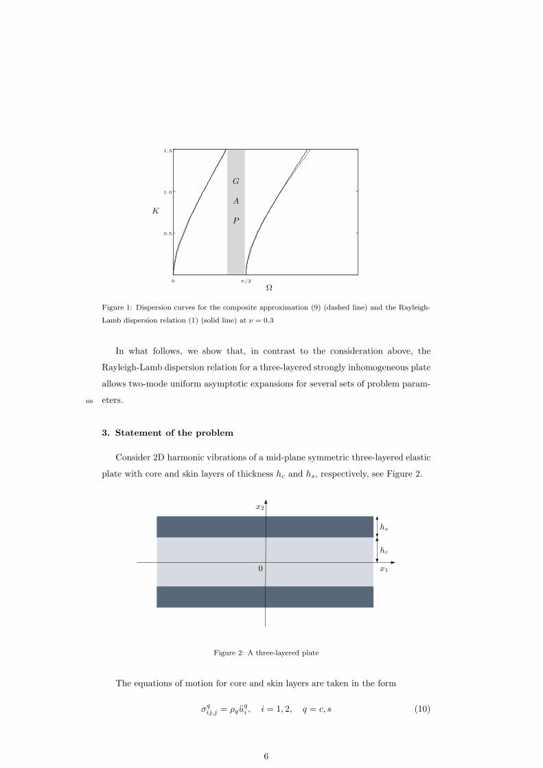
associated gap within the range of validity of the composite dispersion relation (9) is
clearly seen in Figure 1. In this figure the dispersion curves (1) and their composite
approximation (9) are plotted for κ = 0.53, corresponding to the Poisson ratio95
ν = 0.3.
5
0
0.5
1.0
1.5
Ω
K
π/2
G
A
P
Figure 1: Dispersion curves for the composite approximation (9) (dashed line) and the Rayleigh-
Lamb dispersion relation (1) (solid line) at ν = 0.3
In what follows, we show that, in contrast to the consideration above, the
Rayleigh-Lamb dispersion relation for a three-layered strongly inhomogeneous plate
allows two-mode uniform asymptotic expansions for several sets of problem param-
eters.100
3. Statement of the problem
Consider 2D harmonic vibrations of a mid-plane symmetric three-layered elastic
plate with core and skin layers of thickness hc and hs, respectively, see Figure 2.
x2
x1
hc
hs
0
Figure 2: A three-layered plate
The equations of motion for core and skin layers are taken in the form
σqij,j = ρqu
qi , i = 1, 2, q = c, s (10)
6

with the index q taking the values q = c and q = s for the core and skin layers,
respectively; summation over the repeated suffixes is assumed. Here σqij are stresses,105
ui are displacements, ρq are volume mass densities.
The constitutive relations for a linearly isotropic material are given by
σqij = λqε
qkkδij + 2µqε
qij , (11)
with
εqij =1
2(uq
i,j + uqj,i), q = c, s, (12)
where εqij are strains, and λq and µq are the Lame parameters.
The traction free boundary conditions
σs12 = σs
22 = 0 (13)
along the faces x2 = ±(hc+hs) are imposed, together with the continuity conditions
σc12 = σs
12, σc22 = σs
22, uc1 = us
1, uc2 = us
2 (14)
along the interfaces x2 = ±hc.
Let us define the dimensionless frequency Ω and wave number K as
Ω =ωhc
c2c, K = khc, (15)
and introduce the dimensionless parameters
h =hs
hc, ε =
µc
µs, r =
ρcρs
, (16)
expressing the contrast in thickness, stiffness and density of the core and skin layers.
The dispersion relation for the antisymmetric modes of the plate governed by
the equations above, can be written as, e.g. see Lee & Chang (1979),
4K2h3αsβsF4 [F1F2CβcSαc − 2αcβc(ε− 1)F3CαcSβc ]+
hαsβsCαsCβs
[4αcβcK
2(h4F 2
3 + F42(ε− 1)2
)CαcSβc−
(4K4h4F 2
2 + F42F 2
1
)SαcCβc
]+
CβsSαsεβs(β2s −K2h2)(β2
c −K2)[4α2
sβcK2h2SαcSβc − F4
2αcCαcCβc
]+
CαsSβsεαs(β2s −K2h2)(β2
c −K2)[4αcβ
2sK
2h2CαcCβc − F42βcSαcSβc
]+
h3SαsSβs
[(4α2
sβ2sK
2F 21 +K2F4
2F 22
)CβcSαc−
αcβc
(16α2
sβ2s (ε− 1)2K4 + F4
2F 23
)CαcSβc
]= 0,
(17)
7

where
F1 = 2(ε− 1)K2 − εΩ2,
F2 = 2(ε− 1)K2 +ε(1− r)
rΩ2,
F3 = 2(ε− 1)K2 +ε
rΩ2,
F4 = β2s +K2h2,
(18)
and
α2c = K2 − κ
2cΩ
2, α2s = h2
(
K2 − εκ2s
rΩ2
)
,
β2c = K2 − Ω2, βs = h2
(
K2 − ε
rΩ2
)
.
(19)
In the above Cαq = cosh(αq), Cβq = cosh(βq), Sαq = sinh(αq), Sβq = sinh(βq), and
κq = c2q/c1q with
c21q =λq + 2µq
ρq, c22q =
µq
ρq, q = c, s. (20)
On introducing the dimensionless variable χ = x2/hc the displacements of the
core (|χ| ≤ 1) and skins (1 ≤ |χ| ≤ 1 + h) are given by
u1c = iKAc sinh(αcχ)− βcBc sinh(βcχ),
u2c = αcAc cosh(αcχ) + iKBc cosh(βcχ),(21)
and
u1s = iK[As sinh(θsχ) +Bs cosh(θsχ)]− κs[D cosh(κsχ) + sinh(κsχ)],
u2s = θs[As cosh(θsχ) +Bs sinh(θsχ)] + iK[D sinh(κsχ) + cosh(κsχ)],(22)
with θs = αs/h, κs = βs/h and the constants Ac, As, Bc, Bs, and D presented in110
Appendix A.
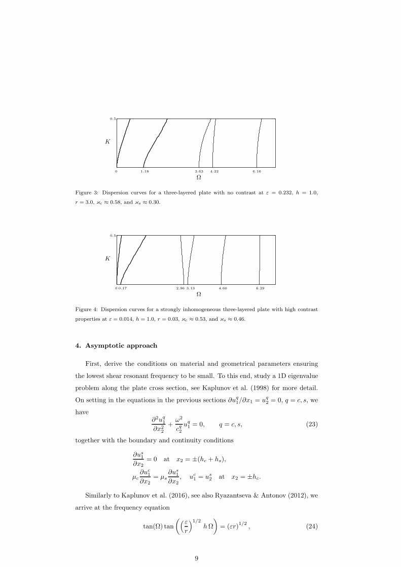
The dispersion curves for two sets of problem parameters are demonstrated in
Figure 3 (ε = 0.232, h = 1.0, r = 3.0, κc ≈ 0.58, and κs ≈ 0.30) and in Figure 4
(ε = 0.014, h = 1.0, r = 0.03, κc ≈ 0.53, and κs ≈ 0.46). Numerical data in Figure
3 is similar to that for a homogeneous plate, see Figure 1, whereas the lowest shear115
thickness resonance Ω = 0.17 being the cut-off of the first harmonic in Figure 4 is
close to zero. This is due to a high contrast in density and stiffness of the core and
skin layers, resulting in the small parameters r and ε defined by (16).
The consideration below is centered around a high-contrast plate, for which
the value of the lowest thickness shear resonance is asymptotically small. In this120
case we may expect that not only the fundamental vibration mode, but also the
first harmonic appear in the low frequency domain. This is not a feature of a
homogeneous plate, for which the first harmonic arises only at Ω ∼ 1, see (7).
8
0 1.18 3.63 4.22 6.16
0.5
K
Ω
Figure 3: Dispersion curves for a three-layered plate with no contrast at ε = 0.232, h = 1.0,
r = 3.0, κc ≈ 0.58, and κs ≈ 0.30.
0
0.5
0.17 2.96 3.13 4.60 6.29
K
Ω
Figure 4: Dispersion curves for a strongly inhomogeneous three-layered plate with high contrast
properties at ε = 0.014, h = 1.0, r = 0.03, κc ≈ 0.53, and κs ≈ 0.46.
4. Asymptotic approach
First, derive the conditions on material and geometrical parameters ensuring
the lowest shear resonant frequency to be small. To this end, study a 1D eigenvalue
problem along the plate cross section, see Kaplunov et al. (1998) for more detail.
On setting in the equations in the previous sections ∂uq1/∂x1 = uq
2 = 0, q = c, s, we
have∂2uq
1
∂x22
+ω2
cq2uq1 = 0, q = c, s, (23)
together with the boundary and continuity conditions
∂us1
∂x2
= 0 at x2 = ±(hc + hs),
µc∂uc
1
∂x2
= µs∂us
1
∂x2
, uc1 = us
2 at x2 = ±hc.
Similarly to Kaplunov et al. (2016), see also Ryazantseva & Antonov (2012), we
arrive at the frequency equation
tan(Ω) tan
((ε
r
)1/2
hΩ
)
= (εr)1/2
, (24)
9

inferring that for the contrast parameters satisfying
r ≪ h ≪ ε−1, (25)
the lowest eigenvalue is small, given at leading order by
Ωsh ≈( r
h
)1/2
≪ 1. (26)
At leading order the associated eigensolution has the following piecewise linear
variation across the thickness, see Figure 5,
ush1 =
χ, for |χ| ≤ 1
1, for 1 ≤ |χ| ≤ 1 + h,
(27)
with χ = x2/hc, which is typical for the so-called global low-frequency behaviour125
defined in Kaplunov et al. (2016). It is worth noting that under the conditions (25)
the eigenmode (27) is the only one demonstrating piecewise linear variation across
the plate thickness.
|χ|
ush1
1.0
0 1.0 2.0
Figure 5: The lowest shear eigenmode (27)
Let us derive the long-wave low-frequency asymptotic expansions of the tran-
scendental Rayleigh-Lamb equation (17) over the parameter range (25) assuming
that
K(1 + h) ≪ 1, Ω
(
1 + h(ε
r
)1/2)
≪ 1. (28)
In this case the hyperbolic functions in (17) may be expanded into asymptotic series,
finally resulting in the polynomial dispersion relation
γ1Ω2 + γ2K
4 + γ3K2Ω2 + γ4K
6 + γ5Ω4 + γ6K
4Ω2 + γ7K8+
γ8K2Ω4 + γ9K
6Ω2 + γ10K10 + ... = 0,
(29)
10
where the coefficients γi are given explicitly in Appendix B.
Next, we express the contrast parameters r and h in (16) through ε as
h ∼ εa, r ∼ εb, (30)
not making any preliminary assumptions regarding the asymptotic order of ε and130
the sign of the constants a and b. Consequently, we estimate the coefficients γi in
(29) as γi → Giεc, where Gi ∼ 1 and c is a constant.
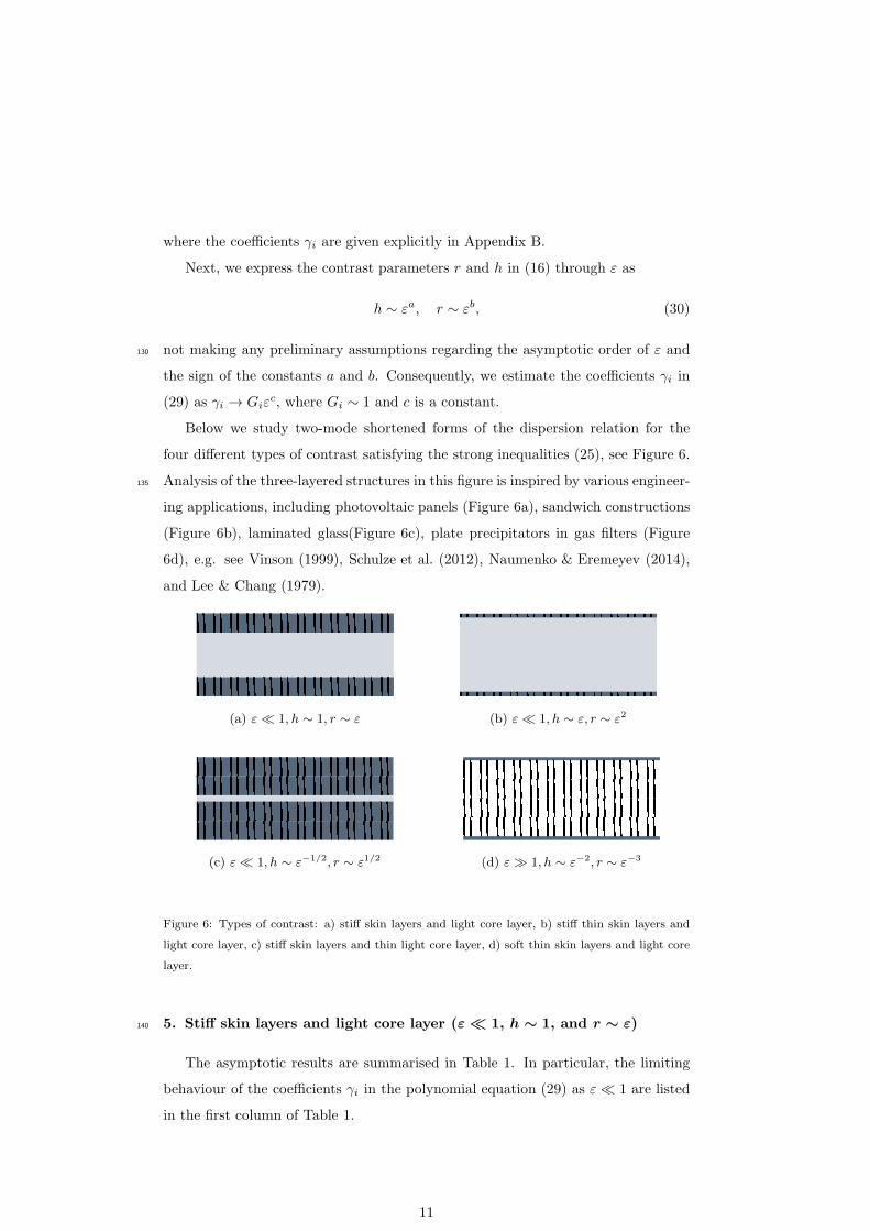
Below we study two-mode shortened forms of the dispersion relation for the
four different types of contrast satisfying the strong inequalities (25), see Figure 6.
Analysis of the three-layered structures in this figure is inspired by various engineer-135
ing applications, including photovoltaic panels (Figure 6a), sandwich constructions
(Figure 6b), laminated glass(Figure 6c), plate precipitators in gas filters (Figure
6d), e.g. see Vinson (1999), Schulze et al. (2012), Naumenko & Eremeyev (2014),
and Lee & Chang (1979).
(a) ε ≪ 1, h ∼ 1, r ∼ ε (b) ε ≪ 1, h ∼ ε, r ∼ ε2
(c) ε ≪ 1, h ∼ ε−1/2, r ∼ ε1/2 (d) ε ≫ 1, h ∼ ε−2, r ∼ ε−3
Figure 6: Types of contrast: a) stiff skin layers and light core layer, b) stiff thin skin layers and
light core layer, c) stiff skin layers and thin light core layer, d) soft thin skin layers and light core
layer.
5. Stiff skin layers and light core layer (ε ≪ 1, h ∼ 1, and r ∼ ε)140
The asymptotic results are summarised in Table 1. In particular, the limiting
behaviour of the coefficients γi in the polynomial equation (29) as ε ≪ 1 are listed
in the first column of Table 1.
11

Order of γi Terms
Fundamental mode Harmonic
K ∼ Ω1/2 K ∼(Ω2 − Ω2
sh
)1/2
Ω ≪ 1 Ωsh ≤ Ω ≪ 1
γ1 ∼ ε γ1Ω2 εK4 ε(ε+K2)
γ2 ∼ ε γ2K4 εK4 εK4
γ3 ∼ 1 γ3K2Ω2 K6 K2(ε+K2)
γ4 ∼ 1 γ4K6 K6 K6
γ5 ∼ 1 γ5Ω4 K8 (ε+K2)2
γ6 ∼ 1 γ6K4Ω2 K8 K4(ε+K2)
γ7 ∼ 1 γ7K8 K8 K8
γ8 ∼ 1 γ8Ω4K2 K10 K2(ε+K2)2
γ9 ∼ 1 γ9K6Ω2 K10 K6(ε+K2)
γ10 ∼ 1 γ10K10 K10 K10
Table 1: Asymptotic behaviour at ε ≪ 1, h ∼ 1, and r ∼ ε
The expressions through the wave number are displayed in the third column for
the fundamental mode and in the fourth column for the first harmonic, for which145
the cut-off frequency is Ωsh ∼ ε1/2 according to (26), see (28).
Let us neglect all of the asymptotically secondary terms at K ≪ 1 in the second
column of Table 1, using the data from the first, third, and fourth columns. Then,
we get
εG1Ω2 + εG2K
4 +G3K2Ω2 +G4K
6 +G5Ω4 = 0, (31)
where at leading order
G1 = −h6
r30, G2 = −4
3
h6(κ2s − 1)(h2 + 3h+ 3)
r20, G3 =
4h7(κ2s − 1)
r30,
G4 =4
3
h9(κ2s − 1)2
r20, G5 =
h7
r40,
(32)
with r0 = r/ε.
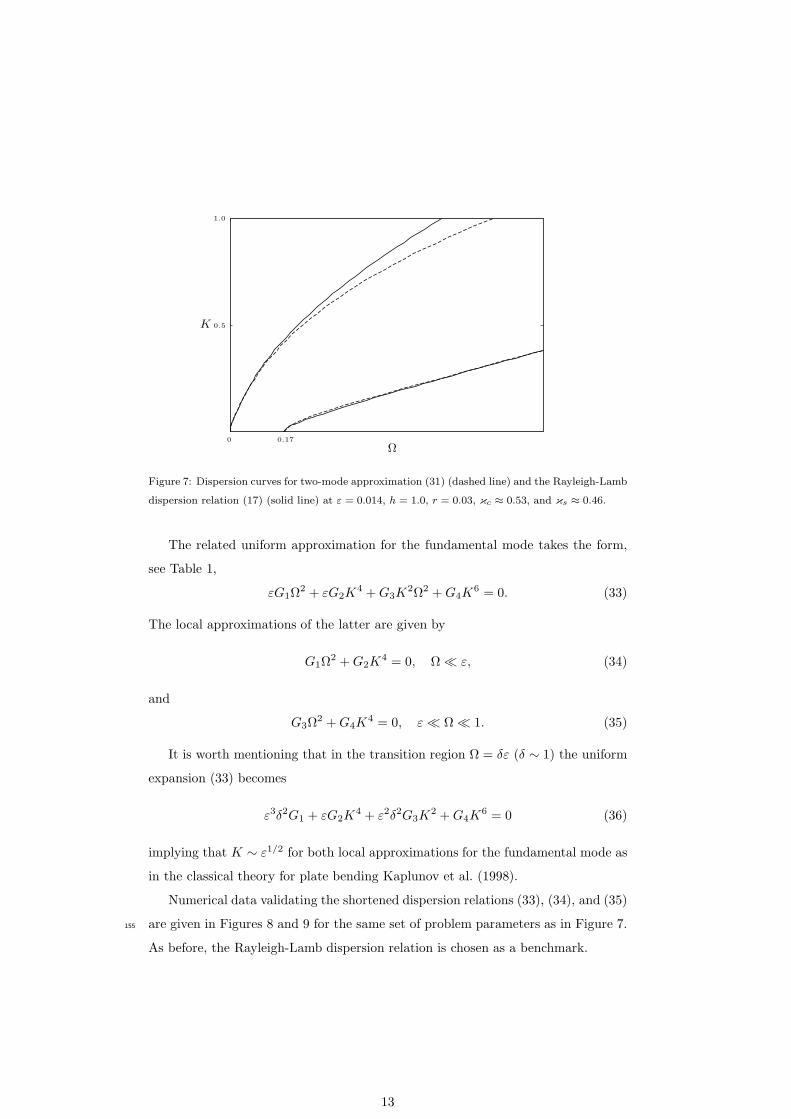
This is a uniform two-mode expansion of the Rayleigh-Lamb dispersion equation,
valid over the entire low-frequency range Ω ≪ 1 in (28) for both the fundamental
mode and the first harmonic, see the numerical illustration in Figure 7 for ε = 0.014,150
h = 1.0, r = 0.03, κc ≈ 0.53, and κs ≈ 0.46.
12
Ω
K 0.5
1.0
0 0.17
Figure 7: Dispersion curves for two-mode approximation (31) (dashed line) and the Rayleigh-Lamb
dispersion relation (17) (solid line) at ε = 0.014, h = 1.0, r = 0.03, κc ≈ 0.53, and κs ≈ 0.46.
The related uniform approximation for the fundamental mode takes the form,
see Table 1,
εG1Ω2 + εG2K
4 +G3K2Ω2 +G4K
6 = 0. (33)
The local approximations of the latter are given by
G1Ω2 +G2K
4 = 0, Ω ≪ ε, (34)
and
G3Ω2 +G4K
4 = 0, ε ≪ Ω ≪ 1. (35)
It is worth mentioning that in the transition region Ω = δε (δ ∼ 1) the uniform
expansion (33) becomes
ε3δ2G1 + εG2K4 + ε2δ2G3K
2 +G4K6 = 0 (36)
implying that K ∼ ε1/2 for both local approximations for the fundamental mode as
in the classical theory for plate bending Kaplunov et al. (1998).
Numerical data validating the shortened dispersion relations (33), (34), and (35)
are given in Figures 8 and 9 for the same set of problem parameters as in Figure 7.155
As before, the Rayleigh-Lamb dispersion relation is chosen as a benchmark.
13
Ω
K 0.5
1.0
0 0.5
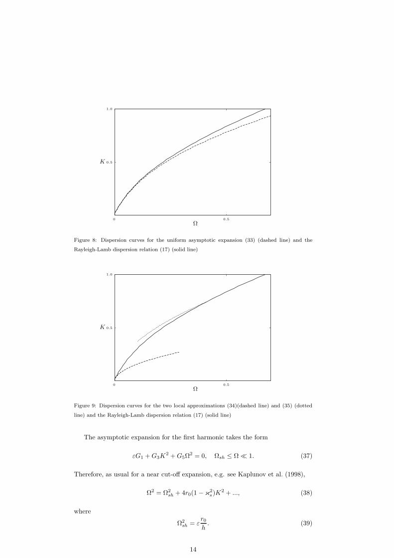
Figure 8: Dispersion curves for the uniform asymptotic expansion (33) (dashed line) and the
Rayleigh-Lamb dispersion relation (17) (solid line)
Ω
K 0.5
1.0
0 0.5
Figure 9: Dispersion curves for the two local approximations (34)(dashed line) and (35) (dotted
line) and the Rayleigh-Lamb dispersion relation (17) (solid line)
The asymptotic expansion for the first harmonic takes the form
εG1 +G3K2 +G5Ω
2 = 0, Ωsh ≤ Ω ≪ 1. (37)
Therefore, as usual for a near cut-off expansion, e.g. see Kaplunov et al. (1998),
Ω2 = Ω2sh + 4r0(1 − κ
2s )K
2 + ..., (38)
where
Ω2sh = ε
r0h. (39)
14
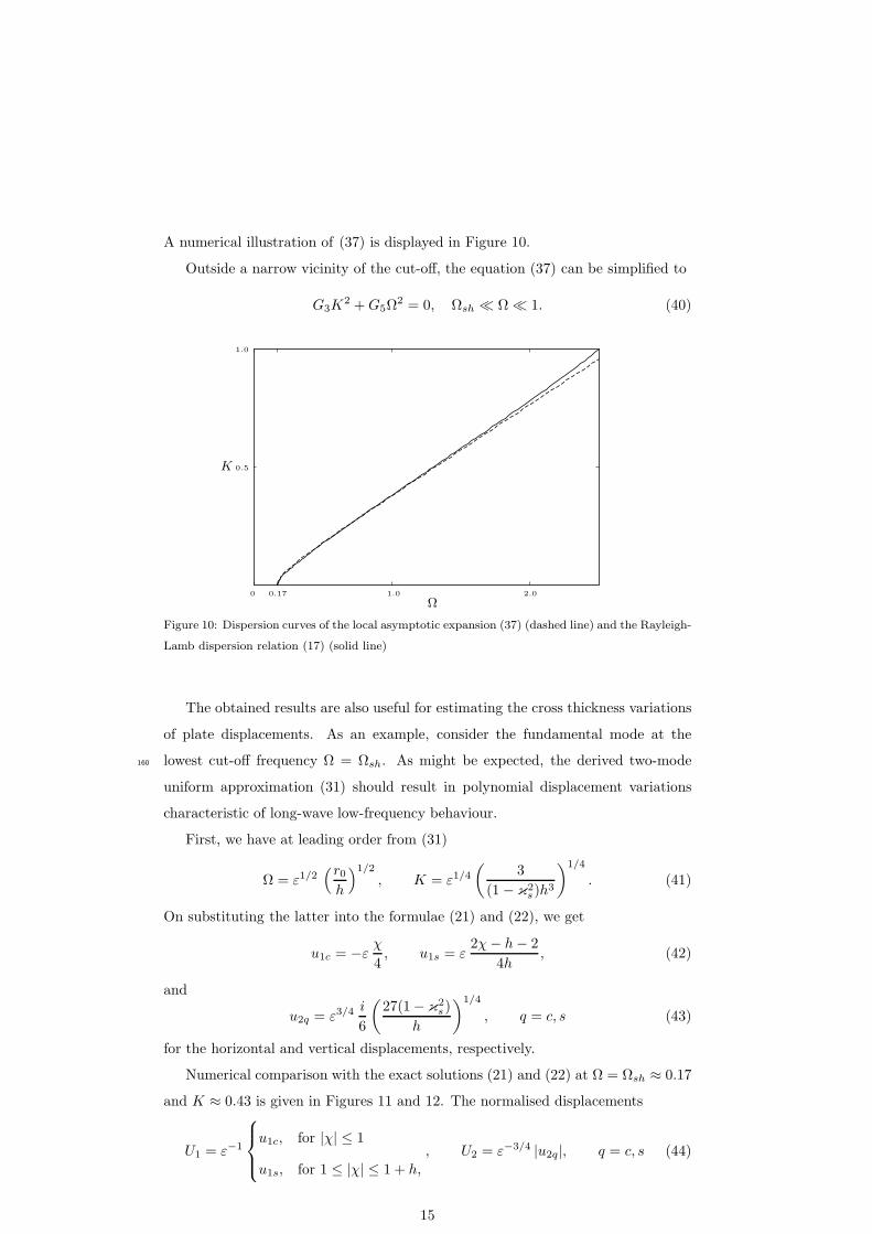
A numerical illustration of (37) is displayed in Figure 10.
Outside a narrow vicinity of the cut-off, the equation (37) can be simplified to
G3K2 +G5Ω
2 = 0, Ωsh ≪ Ω ≪ 1. (40)
Ω
K 0.5
1.0
0 0.17 1.0 2.0
Figure 10: Dispersion curves of the local asymptotic expansion (37) (dashed line) and the Rayleigh-
Lamb dispersion relation (17) (solid line)
The obtained results are also useful for estimating the cross thickness variations
of plate displacements. As an example, consider the fundamental mode at the
lowest cut-off frequency Ω = Ωsh. As might be expected, the derived two-mode160
uniform approximation (31) should result in polynomial displacement variations
characteristic of long-wave low-frequency behaviour.
First, we have at leading order from (31)
Ω = ε1/2(r0h
)1/2
, K = ε1/4(
3
(1 − κ2s)h
3
)1/4
. (41)
On substituting the latter into the formulae (21) and (22), we get
u1c = −εχ
4, u1s = ε
2χ− h− 2
4h, (42)
and
u2q = ε3/4i
6
(27(1− κ
2s )
h
)1/4
, q = c, s (43)
for the horizontal and vertical displacements, respectively.
Numerical comparison with the exact solutions (21) and (22) at Ω = Ωsh ≈ 0.17
and K ≈ 0.43 is given in Figures 11 and 12. The normalised displacements
U1 = ε−1
u1c, for |χ| ≤ 1
u1s, for 1 ≤ |χ| ≤ 1 + h,
, U2 = ε−3/4 |u2q|, q = c, s (44)
15
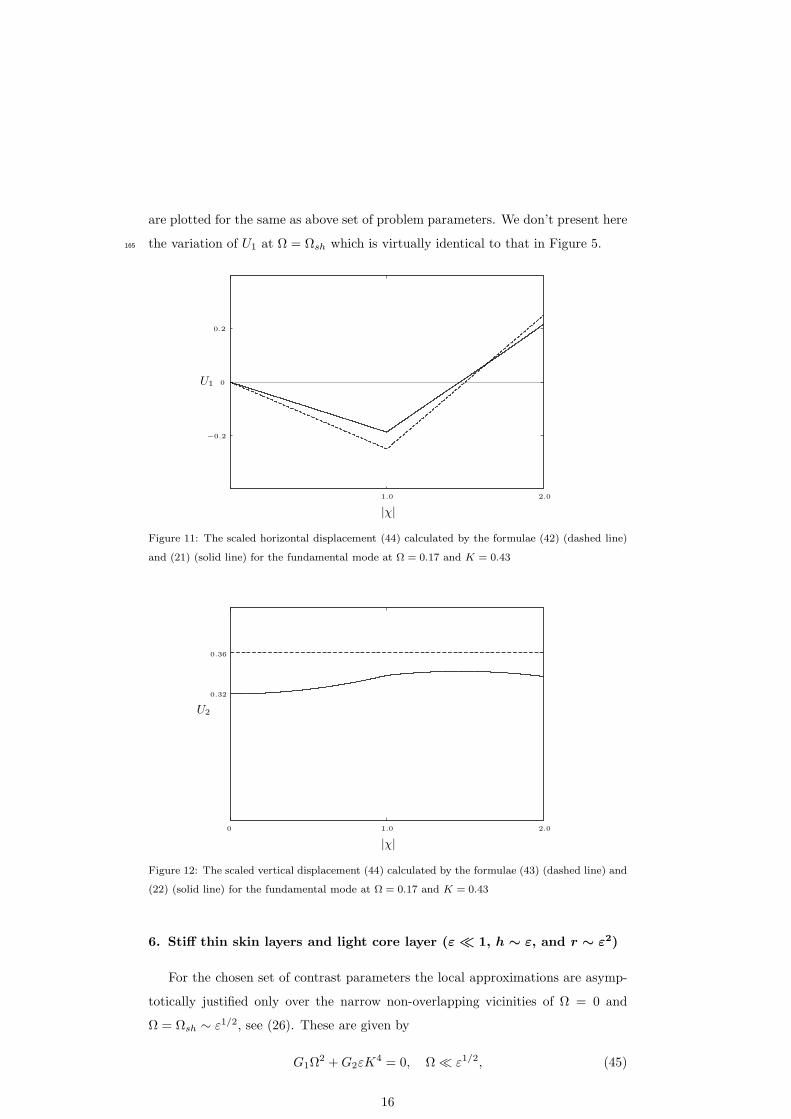
are plotted for the same as above set of problem parameters. We don’t present here
the variation of U1 at Ω = Ωsh which is virtually identical to that in Figure 5.165
|χ|
U1
−0.2
0.2
0
1.0 2.0
Figure 11: The scaled horizontal displacement (44) calculated by the formulae (42) (dashed line)
and (21) (solid line) for the fundamental mode at Ω = 0.17 and K = 0.43
|χ|
U2
0 1.0 2.0
0.32
0.36
Figure 12: The scaled vertical displacement (44) calculated by the formulae (43) (dashed line) and
(22) (solid line) for the fundamental mode at Ω = 0.17 and K = 0.43
6. Stiff thin skin layers and light core layer (ε ≪ 1, h ∼ ε, and r ∼ ε2)
For the chosen set of contrast parameters the local approximations are asymp-
totically justified only over the narrow non-overlapping vicinities of Ω = 0 and
Ω = Ωsh ∼ ε1/2, see (26). These are given by
G1Ω2 +G2εK
4 = 0, Ω ≪ ε1/2, (45)
16

and
G1ε+ εK2
(
G3 +r0h0
G8
)
+G5Ω2 = 0, Ω− Ωsh ≪ ε1/2, (46)
for the fundamental mode and the first harmonic, respectively, see Table 2. In the
above
G1 = −h60
r30, G2 = −4
3
h50(3h0κ
2s + κ
2c − 3h0 − 1)
r20,
G3 =2h6
0(2h0κ2s − 2h0 − 1)
r30, G5 =
h70
r40, G8 =
1
3
h70(κ
2c + 1)
r40
(47)
and
r0 =r
ε2, h0 =
h
ε. (48)
Order of γi Terms
Fundamental mode Harmonic
K ∼ ε−1/4Ω1/2 K ∼(Ω2 − Ω2
sh
)1/2ε−1/2
Ω ≪ ε1/2 Ω− Ωsh ≪ ε1/2
γ1 ∼ ε4 γ1Ω2 ε5K4 ε5
γ2 ∼ ε5 γ2K4 ε5K4 ε5K4
γ3 ∼ ε4 γ3K2Ω2 ε5K6 ε5K2
γ4 ∼ ε5 γ4K6 ε5K6 ε5K6
γ5 ∼ ε3 γ5Ω4 ε5K8 ε5
γ6 ∼ ε4 γ6K4Ω2 ε5K8 ε5K4
γ7 ∼ ε5 γ7K8 ε5K8 ε5K8
γ8 ∼ ε3 γ8Ω4K2 ε5K10 ε5K2
γ9 ∼ ε4 γ9K6Ω2 ε5K10 ε5K6
γ10 ∼ ε5 γ10K10 ε5K10 ε5K10
Table 2: Asymptotic behaviour at ε ≪ 1, h ∼ ε, and r ∼ ε2
Thus, a uniform two-mode asymptotic expansion, similar to that in the previous
section, can not be constructed. As an alternative, we proceed with a composite
expansion
G1εΩ2 +G2ε
2K4 + εK2Ω2
(
G3 +r0h0
G8
)
+G5Ω4 = 0 (49)
with Ωsh ≈ ε1/2(r0h0
)1/2
, see Van Dyke (1975), Andrianov et al. (2013) and ref-
erences therein. This dispersion equation does not approximate the fundamental
mode near the first shear cut-off, i.e. at Ω ∼ ε1/2. A typical gap in the validity
range of the composite expansion (49), similar to that for a homogeneous plate in170
17
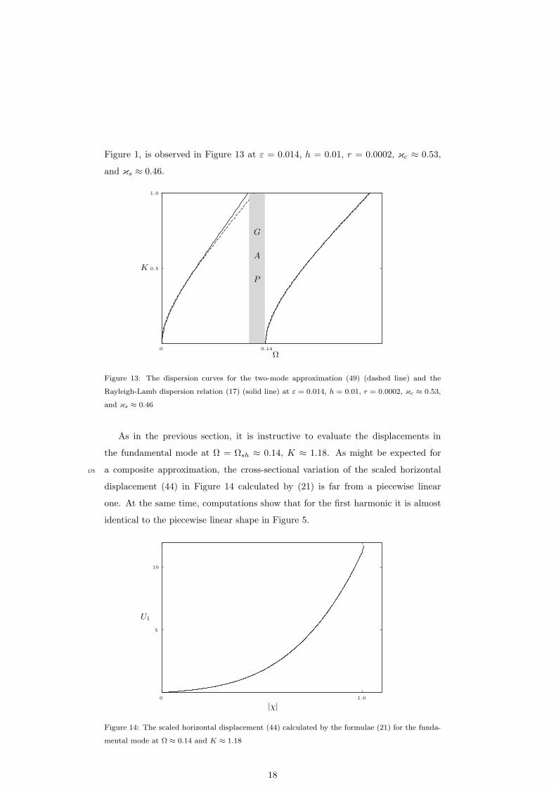
Figure 1, is observed in Figure 13 at ε = 0.014, h = 0.01, r = 0.0002, κc ≈ 0.53,
and κs ≈ 0.46.
Ω
K 0.5
1.0
0 0.14
G
A
P
Figure 13: The dispersion curves for the two-mode approximation (49) (dashed line) and the
Rayleigh-Lamb dispersion relation (17) (solid line) at ε = 0.014, h = 0.01, r = 0.0002, κc ≈ 0.53,
and κs ≈ 0.46
As in the previous section, it is instructive to evaluate the displacements in
the fundamental mode at Ω = Ωsh ≈ 0.14, K ≈ 1.18. As might be expected for
a composite approximation, the cross-sectional variation of the scaled horizontal175
displacement (44) in Figure 14 calculated by (21) is far from a piecewise linear
one. At the same time, computations show that for the first harmonic it is almost
identical to the piecewise linear shape in Figure 5.
|χ|
U1
5
10
0 1.0
Figure 14: The scaled horizontal displacement (44) calculated by the formulae (21) for the funda-
mental mode at Ω ≈ 0.14 and K ≈ 1.18
18
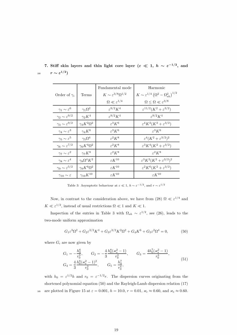
7. Stiff skin layers and thin light core layer (ε ≪ 1, h ∼ ε−1/2, and
r ∼ ε1/2)180
Order of γi Terms
Fundamental mode Harmonic
K ∼ ε3/8Ω1/2 K ∼ ε1/4(Ω2 − Ω2
sh
)1/2
Ω ≪ ε1/4 Ω ≤ Ω ≪ ε3/8
γ1 ∼ ε6 γ1Ω2 ε9/2K4 ε11/2(K2 + ε3/2)
γ2 ∼ ε9/2 γ2K4 ε9/2K4 ε9/2K4
γ3 ∼ ε9/2 γ3K2Ω2 ε3K6 ε4K2(K2 + ε3/2)
γ4 ∼ ε3 γ4K6 ε3K6 ε3K6
γ5 ∼ ε5 γ5Ω4 ε2K8 ε4(K2 + ε3/2)2
γ6 ∼ ε7/2 γ6K4Ω2 ε2K8 ε3K4(K2 + ε3/2)
γ7 ∼ ε2 γ7K8 ε2K8 ε2K8
γ8 ∼ ε4 γ8Ω4K2 εK10 ε3K2(K2 + ε3/2)2
γ9 ∼ ε5/2 γ9K6Ω2 εK10 ε2K6(K2 + ε3/2)
γ10 ∼ ε γ10K10 εK10 εK10
Table 3: Asymptotic behaviour at ε ≪ 1, h ∼ ε−1/2, and r ∼ ε1/2
Now, in contrast to the consideration above, we have from (28) Ω ≪ ε1/4 and
K ≪ ε1/2, instead of usual restrictions Ω ≪ 1 and K ≪ 1.
Inspection of the entries in Table 3 with Ωsh ∼ ε1/2, see (26), leads to the
two-mode uniform approximation
G1ε3Ω2 +G2ε
3/2K4 +G3ε3/2K2Ω2 +G4K
6 +G5ε2Ω4 = 0, (50)
where Gi are now given by
G1 = −h60
r30, G2 = −4
3
h80(κ
2s − 1)
r20, G3 =
4h70(κ
2s − 1)
r30,
G4 =4
3
h90(κ
2s − 1)2
r20, G5 =
h70
r40,
(51)
with h0 = ε1/2h and r0 = ε−1/2r. The dispersion curves originating from the
shortened polynomial equation (50) and the Rayleigh-Lamb dispersion relation (17)
are plotted in Figure 15 at ε = 0.001, h = 10.0, r = 0.01, κc ≈ 0.60, and κs ≈ 0.60.185
19

Ω
K
0.1
0.2
0.3
0 0.03 0.5
Figure 15: The dispersion curves for the uniform two-mode approximation (50) (dashed line) and
the Rayleigh-Lamb dispersion relation (17) (solid line) at ε = 0.001, h = 10.0, r = 0.01, κc ≈ 0.60,
and κs ≈ 0.60
As in Section 6, the uniform approximation (50) involves two local approxima-
tions of the fundamental mode:
G1ε3/2Ω2 +G2K
4 = 0, 0 ≤ Ω ≪ ε3/4 (52)
and
G3ε3/2Ω2 +G4K
4 = 0, ε3/4 ≪ Ω ≪ ε1/4, (53)
as well as the local approximation of the first harmonic
ε3/2G1 +G3K2 + ε1/2G5Ω
2 = 0, Ωsh ≪ Ω ≪ ε3/8. (54)
At Ω ∼ ε3/8 the term with the factor γ6 in Table 3 should be retained. Also, the
first term in the last equation can be neglected at Ω ≫ ε1/2.
20
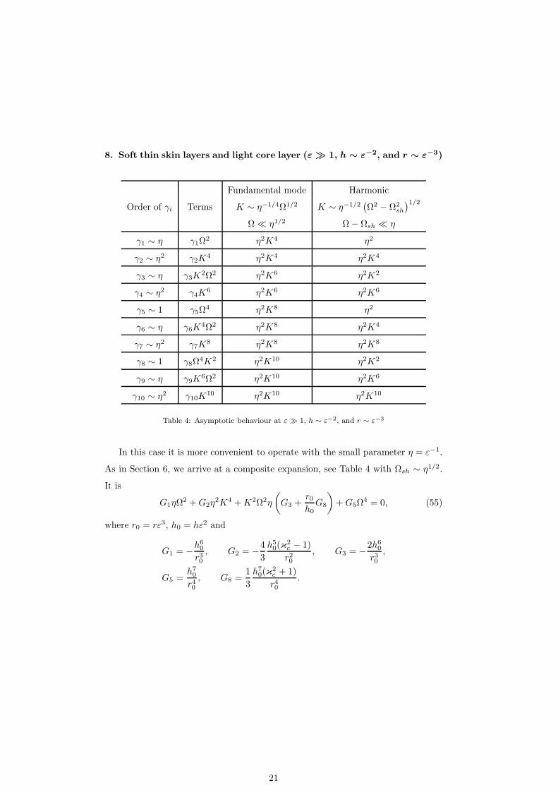
8. Soft thin skin layers and light core layer (ε ≫ 1, h ∼ ε−2, and r ∼ ε
−3)
Order of γi Terms
Fundamental mode Harmonic
K ∼ η−1/4Ω1/2 K ∼ η−1/2(Ω2 − Ω2
sh
)1/2
Ω ≪ η1/2 Ω− Ωsh ≪ η
γ1 ∼ η γ1Ω2 η2K4 η2
γ2 ∼ η2 γ2K4 η2K4 η2K4
γ3 ∼ η γ3K2Ω2 η2K6 η2K2
γ4 ∼ η2 γ4K6 η2K6 η2K6
γ5 ∼ 1 γ5Ω4 η2K8 η2
γ6 ∼ η γ6K4Ω2 η2K8 η2K4
γ7 ∼ η2 γ7K8 η2K8 η2K8
γ8 ∼ 1 γ8Ω4K2 η2K10 η2K2
γ9 ∼ η γ9K6Ω2 η2K10 η2K6
γ10 ∼ η2 γ10K10 η2K10 η2K10
Table 4: Asymptotic behaviour at ε ≫ 1, h ∼ ε−2, and r ∼ ε−3
In this case it is more convenient to operate with the small parameter η = ε−1.
As in Section 6, we arrive at a composite expansion, see Table 4 with Ωsh ∼ η1/2.
It is
G1ηΩ2 +G2η
2K4 +K2Ω2η
(
G3 +r0h0
G8
)
+G5Ω4 = 0, (55)
where r0 = rε3, h0 = hε2 and
G1 = −h60
r30, G2 = −4
3
h50(κ
2c − 1)
r20, G3 = −2h6
0
r30,
G5 =h70
r40, G8 =
1
3
h70(κ
2c + 1)
r40.
21
Ω
K 0.5
1.0
0 0.10
G
A
P
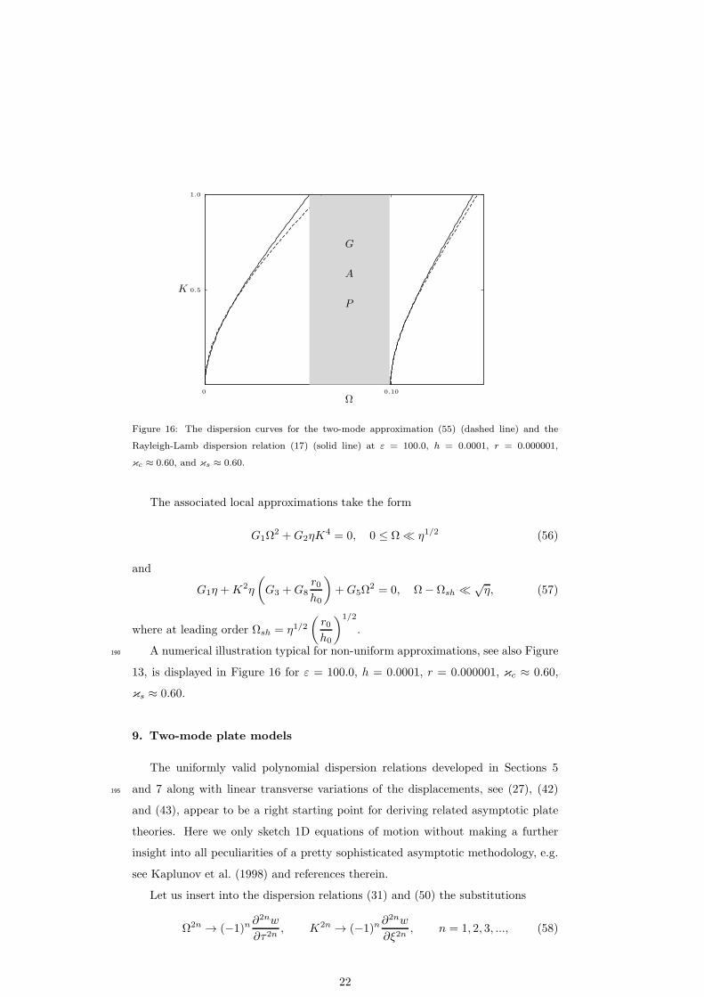
Figure 16: The dispersion curves for the two-mode approximation (55) (dashed line) and the
Rayleigh-Lamb dispersion relation (17) (solid line) at ε = 100.0, h = 0.0001, r = 0.000001,
κc ≈ 0.60, and κs ≈ 0.60.
The associated local approximations take the form
G1Ω2 +G2ηK
4 = 0, 0 ≤ Ω ≪ η1/2 (56)
and
G1η +K2η
(
G3 +G8
r0h0
)
+G5Ω2 = 0, Ω− Ωsh ≪ √
η, (57)
where at leading order Ωsh = η1/2(r0h0
)1/2
.
A numerical illustration typical for non-uniform approximations, see also Figure190
13, is displayed in Figure 16 for ε = 100.0, h = 0.0001, r = 0.000001, κc ≈ 0.60,
κs ≈ 0.60.
9. Two-mode plate models
The uniformly valid polynomial dispersion relations developed in Sections 5
and 7 along with linear transverse variations of the displacements, see (27), (42)195
and (43), appear to be a right starting point for deriving related asymptotic plate
theories. Here we only sketch 1D equations of motion without making a further
insight into all peculiarities of a pretty sophisticated asymptotic methodology, e.g.
see Kaplunov et al. (1998) and references therein.
Let us insert into the dispersion relations (31) and (50) the substitutions
Ω2n → (−1)n∂2nw
∂τ2n, K2n → (−1)n
∂2nw
∂ξ2n, n = 1, 2, 3, ..., (58)
22
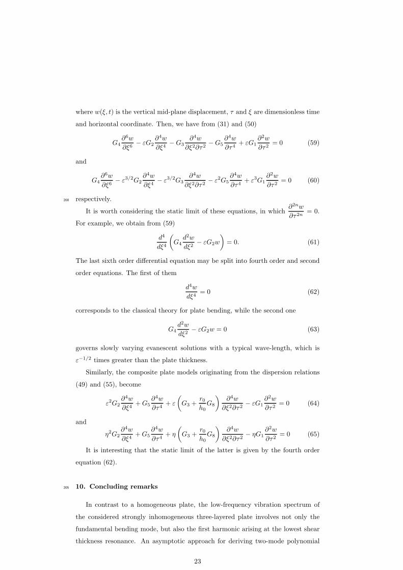
where w(ξ, t) is the vertical mid-plane displacement, τ and ξ are dimensionless time
and horizontal coordinate. Then, we have from (31) and (50)
G4
∂6w
∂ξ6− εG2
∂4w
∂ξ4−G3
∂4w
∂ξ2∂τ2−G5
∂4w
∂τ4+ εG1
∂2w
∂τ2= 0 (59)
and
G4
∂6w
∂ξ6− ε3/2G2
∂4w
∂ξ4− ε3/2G3
∂4w
∂ξ2∂τ2− ε2G5
∂4w
∂τ4+ ε3G1
∂2w
∂τ2= 0 (60)
respectively.200
It is worth considering the static limit of these equations, in which∂2nw
∂τ2n= 0.
For example, we obtain from (59)
d4
dξ4
(
G4
d2w
dξ2− εG2w
)
= 0. (61)
The last sixth order differential equation may be split into fourth order and second
order equations. The first of them
d4w
dξ4= 0 (62)
corresponds to the classical theory for plate bending, while the second one
G4
d2w
dξ2− εG2w = 0 (63)
governs slowly varying evanescent solutions with a typical wave-length, which is
ε−1/2 times greater than the plate thickness.
Similarly, the composite plate models originating from the dispersion relations
(49) and (55), become
ε2G2
∂4w
∂ξ4+G5
∂4w
∂τ4+ ε
(
G3 +r0h0
G8
)∂4w
∂ξ2∂τ2− εG1
∂2w
∂τ2= 0 (64)
and
η2G2
∂4w
∂ξ4+G5
∂4w
∂τ4+ η
(
G3 +r0h0
G8
)∂4w
∂ξ2∂τ2− ηG1
∂2w
∂τ2= 0 (65)
It is interesting that the static limit of the latter is given by the fourth order
equation (62).
10. Concluding remarks205
In contrast to a homogeneous plate, the low-frequency vibration spectrum of
the considered strongly inhomogeneous three-layered plate involves not only the
fundamental bending mode, but also the first harmonic arising at the lowest shear
thickness resonance. An asymptotic approach for deriving two-mode polynomial
23
approximations of the transcendental Rayleigh-Lamb dispersion relation is devel-210
oped. Four types of high contrast inspired by modern industrial applications, are
thoroughly investigated. Two-mode approximations can be both uniform or non-
uniform (composite) depending on contrast parameters. The latter are not asymp-
totically justified for studying the fundamental mode near the lowest shear cut-off.
It is remarkable that the leading order uniform approximations analysed in the215
paper are given by six-order polynomials in wave number, while all the consid-
ered composite approximations are forth-order polynomials. A good agreement of
asymptotic results and the numerical data obtained from the Rayleigh-Lamb equa-
tion is demonstrated.
The 1D partial differential equations corresponding to the shortened polynomial220
dispersion relations, reveal a clear potential for developing more general two-mode
asymptotic models for strongly inhomogeneous layered plates. Such models would
be apparently useful for mathematical justification and refinement of various ad
hoc shear deformation theories, e.g. see Qatu (2004), Reddy (2004). In this case a
key challenge may be concerned with formulation of consistent boundary conditions225
for six-order equations of motion starting from an appropriate version of the Saint-
Venant’s principle, e.g. see Gregory & Wan (1985) , Babenkova & Kaplunov (2004)
and references therein.
The proposed methodology is not restricted to four high-contrast setups of a
three-layered plate considered in the paper. A number of extensions, including230
asymmetric multi-layered structures, subject to a variety of interfacial conditions,
seems to be of interest for advanced technologies. However, one should not always
expect a uniform approximation for a high-contrast scenario.
24
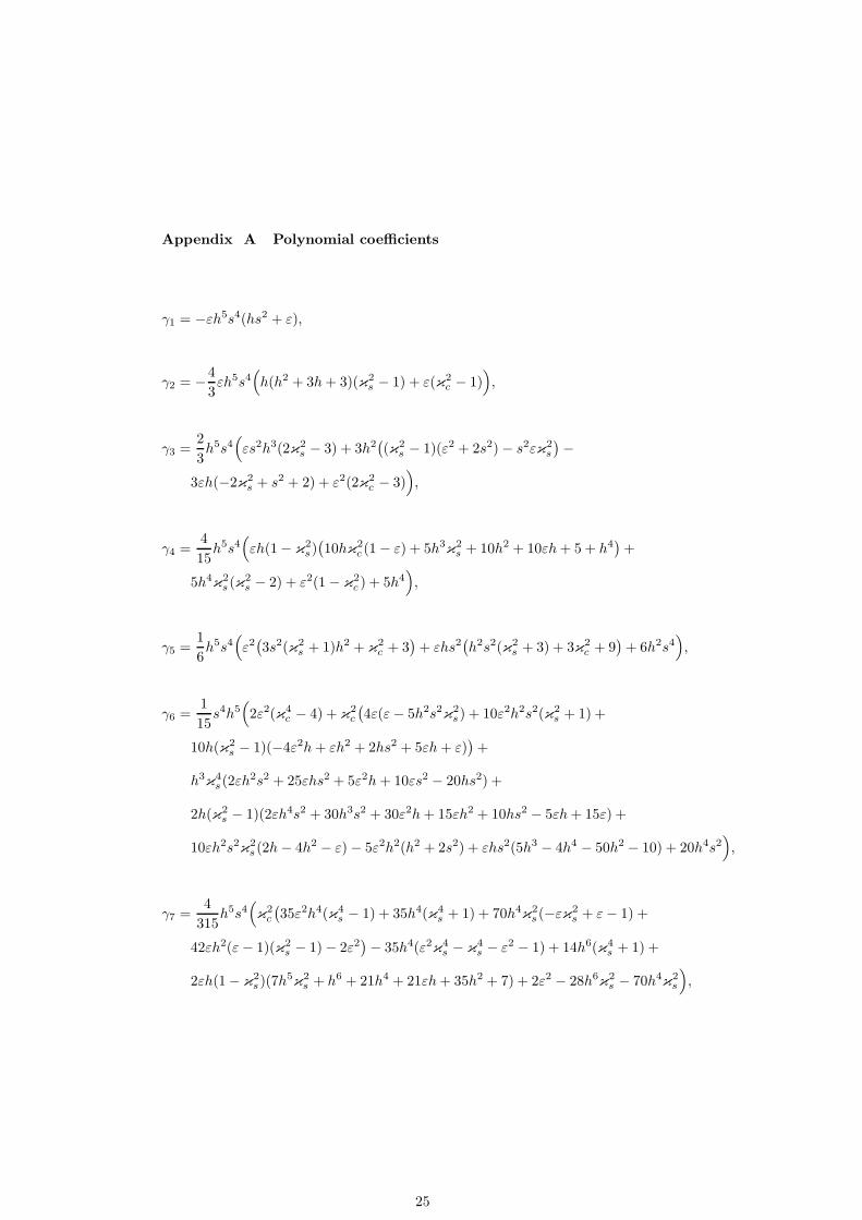
Appendix A Polynomial coefficients
γ1 = −εh5s4(hs2 + ε),
γ2 = −4
3εh5s4
(
h(h2 + 3h+ 3)(κ2s − 1) + ε(κ2
c − 1))
,
γ3 =2
3h5s4
(
εs2h3(2κ2s − 3) + 3h2
((κ2
s − 1)(ε2 + 2s2)− s2εκ2s
)−
3εh(−2κ2s + s2 + 2) + ε2(2κ2
c − 3))
,
γ4 =4
15h5s4
(
εh(1− κ2s)(10hκ2
c (1− ε) + 5h3κ2s + 10h2 + 10εh+ 5 + h4
)+
5h4κ2s (κ
2s − 2) + ε2(1 − κ
2c ) + 5h4
)
,
γ5 =1
6h5s4
(
ε2(3s2(κ2
s + 1)h2 + κ2c + 3
)+ εhs2
(h2s2(κ2
s + 3) + 3κ2c + 9
)+ 6h2s4
)
,
γ6 =1
15s4h5
(
2ε2(κ4c − 4) + κ
2c
(4ε(ε− 5h2s2κ2
s ) + 10ε2h2s2(κ2s + 1) +
10h(κ2s − 1)(−4ε2h+ εh2 + 2hs2 + 5εh+ ε)
)+
h3κ4s (2εh
2s2 + 25εhs2 + 5ε2h+ 10εs2 − 20hs2) +
2h(κ2s − 1)(2εh4s2 + 30h3s2 + 30ε2h+ 15εh2 + 10hs2 − 5εh+ 15ε) +
10εh2s2κ2s (2h− 4h2 − ε)− 5ε2h2(h2 + 2s2) + εhs2(5h3 − 4h4 − 50h2 − 10) + 20h4s2
)
,
γ7 =4
315h5s4
(
κ2c
(35ε2h4(κ4
s − 1) + 35h4(κ4s + 1) + 70h4
κ2s (−εκ2
s + ε− 1) +
42εh2(ε− 1)(κ2s − 1)− 2ε2
)− 35h4(ε2κ4
s − κ4s − ε2 − 1) + 14h6(κ4
s + 1) +
2εh(1− κ2s )(7h
5κ2s + h6 + 21h4 + 21εh+ 35h2 + 7) + 2ε2 − 28h6
κ2s − 70h4
κ2s
)
,
25

γ8 = − 1
30h5s4
(
4ε2κ4c + κ
2c
(10h(κ2
s − 1)(ε2h+ 6hs2 + 2ε) + 20ε2h2s2(κ2s + 1) +
10εh2s2(2h− 5)κ2s − 30h3s2ε− 10h2s4 − 15hs2ε− 3ε2
)+
2h4s4κ4s (2εh+ 5) + h2s2κ2
s (−3εh3s2 − 20εh2s2 + 20h2s2 + 10ε) +
5h(κ2s − 1)(3ε2h3
κ2ss
2 + 6ε2h+ 4hs2 + 4ε) + 10εh2s2(κ2s + 1)(2hκ2
s − 2hs2 − 3ε)−
5εh4s4(κ4s − 1)− 9εh5s4 − 10h4s2ε2 − 40h4s4 − 70h3s2ε− 10h2s4 − 25hs2ε− 9ε2
)
,
γ9 =2h5s4
315
(
2εh7s2(2κ4s + 2κ2
s − 5) + 7h6(ε2(κ4
s − 1) + εs2(2κ6s + 5κ4
s − 10κ2s + 1)−
2s2(κ2s − 1)(κ4
s + 2κ2s − 5)
)+ 21εh5
(3s2κ4
s + (κ2c + 2s2 + 3)κ2
s − 7s2 − κ2c − 3
)+
h4
35ε2(κ4s(3s
2(1 − κ2c )− 2κ2
c + 3) + 3s2κ2s (κ
2c − 1) + 2s2(κ2
c − 1) + 2κ2c − 3
)+
35ε(κ4s (5κ
2cs
2 + 5κ2c − 1) + κ
2s (−8κ2
cs2 − 5κ2
c + 1) + s2κ2c
)−
35(κ2s − 1)
(κ2s (2s
2(κ2c + 1) + 3κ2
c + 1)− 4s2(κ2c + 1)− 3κ2
c − 1)
+
35εh3(κ2s (3κ
2c + 2s2 + 5) + s2κ4
s − 5s2 − 3κ2c − 5
)+
h2
21(
ε2κ2s
(s2(κ2
c − 1) + 8− 2κ4c − 4κ2
c
)+ s2(κ2
c − 1)− 8 + 2κ4c + 4κ2
c
+
ε(κ2s (2κ
4c − 2κ2
cs2 + 7κ2
c − 1) + 1− 2κ4c − 7κ2
c
)+ 2s2(κ2
s − 1)(κ2c + 1)
)
−
14εh(−2κ2s
(κ2c + 2) + s2 + 2κ2
c + 4)+ 2ε2(2κ4
c + 2κ2c − 5)
)
,
γ10 = − 4
2835h5s4
(
εh9(κ2s − 1) + 9h8
(εκ2
s(κ2s − 1)− (κ2
s − 1)2)+ 36εh7(κ2
s − 1)−
42h6(κ2s − 1)
((κ2
c − 1)(κ2s + 1)ε2 − 2εκ2
cκ2s + (κ2
c + 1)(κ2s − 1)
)+
126εh5(κ2s − 1)− 63h4(κ2
s − 1)((κ2
c − 1)(κ2s + 1)ε2 − 2εκ2
cκ2s + (κ2
c + 1)(κ2s − 1)
)+
84εh3(κ2s − 1)− 36εh2(κ2
s − 1)(ε(κ2
c − 1)− κ2c
)+ 9εh(κ2
s − 1) + ε2(κ2c − 1)
)
,
where s2 = ε/r.235
Appendix B Coefficients in formulae (21) and (22)
Ac = a1cD + a2c, Bc = b1cD + b2c, As = a1sD + a2s, Bs = b1sD + b2s,
26
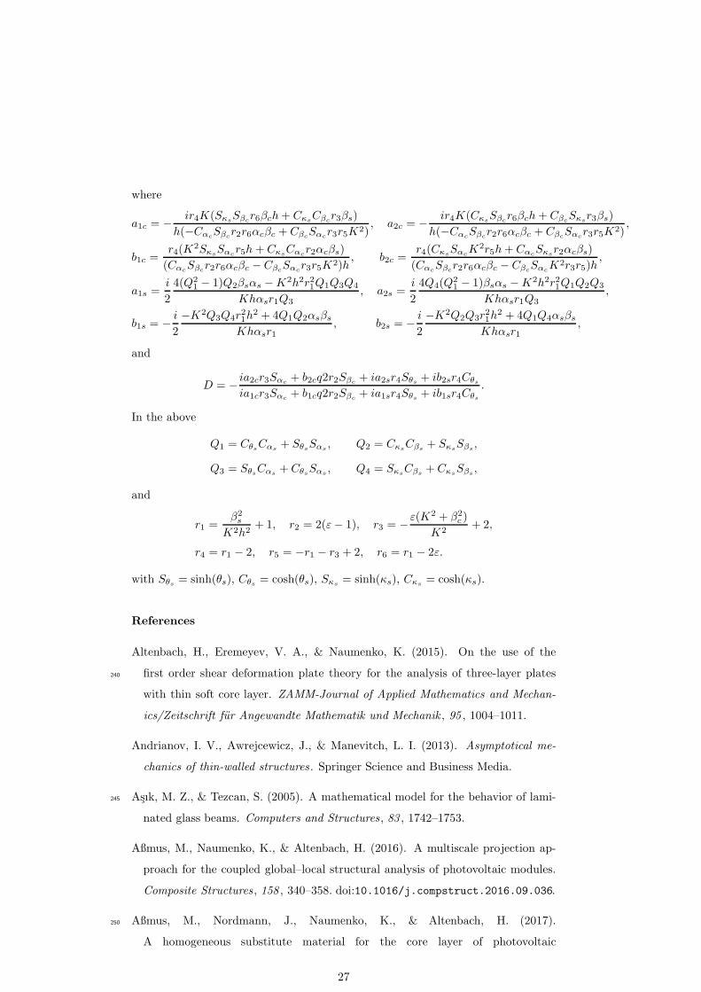
where
a1c = − ir4K(SκsSβcr6βch+ CκsCβcr3βs)
h(−CαcSβcr2r6αcβc + CβcSαcr3r5K2), a2c = − ir4K(CκsSβcr6βch+ CβcSκsr3βs)
h(−CαcSβcr2r6αcβc + CβcSαcr3r5K2),
b1c =r4(K
2SκsSαcr5h+ CκsCαcr2αcβs)
(CαcSβcr2r6αcβc − CβcSαcr3r5K2)h
, b2c =r4(CκsSαcK
2r5h+ CαcSκsr2αcβs)
(CαcSβcr2r6αcβc − CβcSαcK2r3r5)h
,
a1s =i
2
4(Q21 − 1)Q2βsαs −K2h2r21Q1Q3Q4
Khαsr1Q3
, a2s =i
2
4Q4(Q21 − 1)βsαs −K2h2r21Q1Q2Q3
Khαsr1Q3
,
b1s = − i
2
−K2Q3Q4r21h
2 + 4Q1Q2αsβs
Khαsr1, b2s = − i
2
−K2Q2Q3r21h
2 + 4Q1Q4αsβs
Khαsr1,
and
D = − ia2cr3Sαc + b2cq2r2Sβc + ia2sr4Sθs + ib2sr4Cθs
ia1cr3Sαc + b1cq2r2Sβc + ia1sr4Sθs + ib1sr4Cθs
.
In the above
Q1 = CθsCαs + SθsSαs , Q2 = CκsCβs + SκsSβs ,
Q3 = SθsCαs + CθsSαs , Q4 = SκsCβs + CκsSβs ,
and
r1 =β2s
K2h2+ 1, r2 = 2(ε− 1), r3 = −ε(K2 + β2
c )
K2+ 2,
r4 = r1 − 2, r5 = −r1 − r3 + 2, r6 = r1 − 2ε.
with Sθs = sinh(θs), Cθs = cosh(θs), Sκs = sinh(κs), Cκs = cosh(κs).
References
Altenbach, H., Eremeyev, V. A., & Naumenko, K. (2015). On the use of the
first order shear deformation plate theory for the analysis of three-layer plates240
with thin soft core layer. ZAMM-Journal of Applied Mathematics and Mechan-
ics/Zeitschrift fur Angewandte Mathematik und Mechanik , 95 , 1004–1011.
Andrianov, I. V., Awrejcewicz, J., & Manevitch, L. I. (2013). Asymptotical me-
chanics of thin-walled structures . Springer Science and Business Media.
Asık, M. Z., & Tezcan, S. (2005). A mathematical model for the behavior of lami-245
nated glass beams. Computers and Structures , 83 , 1742–1753.
Aßmus, M., Naumenko, K., & Altenbach, H. (2016). A multiscale projection ap-
proach for the coupled global–local structural analysis of photovoltaic modules.
Composite Structures , 158 , 340–358. doi:10.1016/j.compstruct.2016.09.036.
Aßmus, M., Nordmann, J., Naumenko, K., & Altenbach, H. (2017).250
A homogeneous substitute material for the core layer of photovoltaic
27
composite structures. Composites Part B: Engineering, 112 , 353–372.
doi:10.1016/j.compositesb.2016.12.042.
Babenkova, E., & Kaplunov, J. (2004). Low-frequency decay conditions for a semi-
infinite elastic strip. Proceedings of the Royal Society of London A: Mathematical,255
Physical and Engineering Sciences , 460 , 2153–2169.
Berdichevsky, V. (2009). Variational principles of continuum mechanics: I. Funda-
mentals . Springer Science & Business Media.
Berdichevsky, V. L. (2010). An asymptotic theory of sandwich plates. International
Journal of Engineering Science, 48 , 383–404.260
Carrera, E., & Brischetto, S. (2009). A survey with numerical assessment of clas-
sical and refined theories for the analysis of sandwich plates. Applied Mechanics
Reviews , 62 , 010803.
Chapman, C. J. (2013). An asymptotic decoupling method for waves in layered
media. Proceedings of the Royal Society of London A: Mathematical, Physical265
and Engineering Sciences , 469 , 20120659.
Cherdantsev, M., & Cherednichenko, K. D. (2012). Two-scale Γ-convergence of inte-
gral functionals and its application to homogenisation of nonlinear high-contrast
periodic composites. Archive for Rational Mechanics and Analysis , 204 , 445–478.
Craster, R. V., Joseph, L. M., & Kaplunov, J. (2014). Long-wave asymptotic270
theories: the connection between functionally graded waveguides and periodic
media. Wave Motion, 51 , 581–588.
Elishakoff, I., Kaplunov, J., & Nolde, E. (2015). Celebrating the centenary of
Timoshenko’s study of effects of shear deformation and rotary inertia. Applied
Mechanics Reviews , 67 , 060802.275
Figotin, A., & Kuchment, P. (1998). Spectral properties of classical waves in high-
contrast periodic media. SIAM Journal on Applied Mathematics , 58 , 683–702.
Graff, K. F. (2012). Wave motion in elastic solids . Courier Corporation.
Gregory, R. D., & Wan, F. Y. M. (1985). On plate theories and Saint-Venant’s
principle. International Journal of Solids and Structures , 21 , 1005–1024.280
Hohe, J., & Librescu, L. (2004). Advances in the structural modeling of elastic
sandwich panels. Mechanics of Advanced Materials and Structures , 11 , 395–424.
28

Kaplunov, J., & Nobili, A. (2016). Multi-parametric analysis of strongly inho-
mogeneous periodic waveguides with internal cut-off frequencies. Mathematical
Methods in the Applied Sciences , . doi:10.1002/mma.3900.285
Kaplunov, J., Prikazchikov, D., & Sergushova, O. (2016). Multi-parametric analysis
of the lowest natural frequencies of strongly inhomogeneous elastic rods. Journal
of Sound and Vibration, 366 , 264–276.
Kaplunov, J. D., Kossovich, L. Y., & Nolde, E. V. (1998). Dynamics of thin walled
elastic bodies . Academic Press.290
Kreja, I. (2011). A literature review on computational models for laminated com-
posite and sandwich panels. Open Engineering, 1 , 59–80.
Kudaibergenov, A., Nobili, A., & Prikazchikova, L. (2016). On low-frequency vibra-
tions of a composite string with contrast properties for energy scavenging fabric
devices. Journal of Mechanics of Materials and Structures , 11 , 231–243.295
Le, K. C. (1999). Vibrations of shells and rods . Springer Berlin.
Lee, P., & Chang, N. (1979). Harmonic waves in elastic sandwich plates. Journal
of Elasticity, 9 , 51–69.
Martin, T. P., Layman, C. N., Moore, K. M., & Orris, G. J. (2012). Elastic
shells with high-contrast material properties as acoustic metamaterial compo-300
nents. Physical Review B , 85 , 161103.
Milton, G. W. (2002). The theory of composites . Cambridge University Press.
Naumenko, K., & Eremeyev, V. A. (2014). A layer-wise theory for laminated glass
and photovoltaic panels. Composite Structures , 112 , 283–291.
Qatu, M. S. (2004). Vibration of laminated shells and plates . Elsevier.305
Reddy, J. N. (2004). Mechanics of laminated composite plates and shells: theory
and analysis . CRC Press.
Ryazantseva, M. Y., & Antonov, F. K. (2012). Harmonic running waves in sandwich
plates. International Journal of Engineering Science, 59 , 184–192.
Schulze, S. H., Pander, M., Naumenko, K., & Altenbach, H. (2012). Analysis of310
laminated glass beams for photovoltaic applications. International Journal of
Solids and Structures , 49 , 2027–2036.
29

Smyshlyaev, V. P. (2009). Propagation and localization of elastic waves in highly
anisotropic periodic composites via two-scale homogenization. Mechanics of Ma-
terials , 41 , 434–447.315
Tovstik, P. E., & Tovstik, T. P. (2016). Generalized Timoshenko-Reissner mod-
els for beams and plates, strongly heterogeneous in the thickness direction.
ZAMM-Journal of Applied Mathematics and Mechanics/Zeitschrift fur Ange-
wandte Mathematik und Mechanik , . doi:10.1002/zamm.201600052.
Van Dyke, M. (1975). Perturbation methods in fluid mechanics . Parabolic Press,320
Stanford, CA.
Vinson, J. R. (1999). The behavior of sandwich structures of isotropic and composite
materials . CRC Press.
Wang, C. M., Reddy, J. N., & Lee, K. H. (2000). Shear deformable beams and
plates: Relationships with classical solutions . Elsevier.325
30