holistically-nested edge detectionpages.ucsd.edu/~ztu/publication/hed_ijcv.pdf ·...
TRANSCRIPT

Noname manuscript No.(will be inserted by the editor)
Holistically-Nested Edge Detection
Saining Xie · Zhuowen Tu
Received: date / Accepted: date
Abstract We develop a new edge detection algorithm that addresses twoimportant issues in this long-standing vision problem: (1) holistic image train-ing and prediction; and (2) multi-scale and multi-level feature learning. Ourproposed method, holistically-nested edge detection (HED), performs image-to-image prediction by means of a deep learning model that leverages fullyconvolutional neural networks and deeply-supervised nets. HED automaticallylearns rich hierarchical representations (guided by deep supervision on side re-sponses) that are important in order to resolve the challenging ambiguity inedge and object boundary detection. We significantly advance the state-of-the-art on the BSDS500 dataset (ODS F-score of 0.790) and the NYU Depthdataset (ODS F-score of 0.746), and do so with an improved speed (0.4s perimage) that is orders of magnitude faster than some CNN-based edge detec-tion algorithms developed before HED. We also observe encouraging results onother boundary detection benchmark datasets such as Multicue and PASCAL-Context.
1 Introduction
In this paper, we address the problem of detecting edges and object bound-aries in natural images. This problem is both fundamental and of great impor-tance to a variety of computer vision areas ranging from traditional tasks suchas visual saliency, segmentation, object detection/recognition, tracking andmotion analysis, medical imaging, structure-from-motion and 3D reconstruc-tion, to modern applications like autonomous driving, mobile computing, andimage-to-text analysis. It has been long understood that precisely localizing
9500 Gilman DriveLa Jolla, CA 92093-0515 USATel.: +1-858-822-0908Fax: +1-858-534-1128E-mail: {s9xie,ztu}@ucsd.edu
2 Saining Xie, Zhuowen Tu
edges in natural images involves visual perception of various “levels” (Hubeland Wiesel, 1962; Marr and Hildreth, 1980). A relatively comprehensive datacollection and cognitive study (Martin et al, 2004) shows that while differ-ent human subjects do have somewhat different preferences regarding whereto place the edges and boundaries, there was nonetheless impressive consis-tency between subjects, e.g. reaching an F-score 0.80 in the consistency study(Martin et al, 2004).
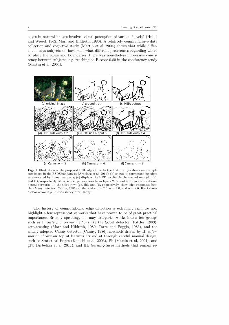
(a) original image (b) ground truth (c) HED: output
(d) HED: side output 2 (e) HED: side output 3 (f) HED: side output 4
(h) Canny: 𝜎𝜎 = 4 (i) Canny: 𝜎𝜎 = 8(g) Canny: 𝜎𝜎 = 2
Fig. 1 Illustration of the proposed HED algorithm. In the first row: (a) shows an exampletest image in the BSDS500 dataset (Arbelaez et al, 2011); (b) shows its corresponding edgesas annotated by human subjects; (c) displays the HED results. In the second row: (d), (e),and (f), respectively, show side edge responses from layers 2, 3, and 4 of our convolutionalneural networks. In the third row: (g), (h), and (i), respectively, show edge responses fromthe Canny detector (Canny, 1986) at the scales σ = 2.0, σ = 4.0, and σ = 8.0. HED showsa clear advantage in consistency over Canny.
The history of computational edge detection is extremely rich; we nowhighlight a few representative works that have proven to be of great practicalimportance. Broadly speaking, one may categorize works into a few groupssuch as I: early pioneering methods like the Sobel detector (Kittler, 1983),zero-crossing (Marr and Hildreth, 1980; Torre and Poggio, 1986), and thewidely adopted Canny detector (Canny, 1986); methods driven by II: infor-mation theory on top of features arrived at through careful manual design,such as Statistical Edges (Konishi et al, 2003), Pb (Martin et al, 2004), andgPb (Arbelaez et al, 2011); and III: learning-based methods that remain re-
Holistically-Nested Edge Detection 3
liant on features of human design, such as BEL (Dollar et al, 2006), Multi-scale(Ren, 2008), Sketch Tokens (Lim et al, 2013), and Structured Edges (Dollarand Zitnick, 2015). In addition, there has been a recent wave of developmentusing Convolutional Neural Networks that emphasize the importance of au-tomatic hierarchical feature learning, including N4-Fields (Ganin and Lem-pitsky, 2014), DeepContour (Shen et al, 2015), DeepEdge (Bertasius et al,2015), and CSCNN (Hwang and Liu, 2015). Prior to this explosive develop-ment in deep learning, the Structured Edges method (typically abbreviatedSE) (Dollar and Zitnick, 2015) emerged as one of the most celebrated systemsfor edge detection, thanks to its state-of-the-art performance on the BSDS500dataset (Martin et al, 2004; Arbelaez et al, 2011) (with, e.g., F-score of 0.746)and its practically significant speed of 2.5 frames per second.
Convolutional neural networks (CNN) (LeCun et al, 1989) have achieved agreat success in automatically learning thousands (or even millions or billions)of features for pattern recognition, under the paradigm of image-to-class clas-sification (e.g. predicting which category an image belongs to (Russakovskyet al, 2014)) or patch-to-class classification (e.g predicting which object an im-age patch contains (Girshick et al, 2014)). CNN-based edge detection methodsbefore HED (Ganin and Lempitsky, 2014; Shen et al, 2015; Bertasius et al,2015; Hwang and Liu, 2015) mostly follow a patch-to-class paradigm, which ispatch-centric. These patch-centric approaches fall into the category of “sliding-window” methods that perform prediction by considering dense, overlappingwindows of the image, often centered at every pixel; this creates a big bot-tleneck in both training and testing; for example, time to detect edges in onestatic image for these methods ranges from several seconds (Ganin and Lem-pitsky, 2014) to a few hours (Bertasius et al, 2015) (even when using modernGPUs). Recently proposed fully convolutional neural networks (FCN) (Longet al, 2015), targeted for the task of semantic image labeling, instead pointsto a promising direction of performing training/testing for the entire imagealtogether, which is under a image-centric paradigm. Applying FCN to theedge detection problem however produces an unsatisfactory result (e.g. F-score 0.745 on BSDS500) as edges observe strong multi-scale aspects that isquite different from semantic labeling. In this regard, the deeply-supervisednets method (DSN) (Lee et al, 2015) provides a principled and clean solu-tion for multi-scale learning and fusion where supervised information is jointlyenforced in the individual convolutional layers during training.
Motivated by fully convolutional networks (Long et al, 2015) and deeply-supervised nets (Lee et al, 2015), we develop an end-to-end edge detectionsystem, holistically-nested edge detection (HED), that automatically learnsthe type of rich hierarchical features that are crucial if we are to approach thehuman ability to resolve ambiguity in natural image edge and object bound-ary detection. We use the term “holistic”, because HED, despite not explicitlymodeling structured output, aims to train and predict edges in an image-to-image fashion. With “nested”, we emphasize the inherited and progressivelyrefined edge maps produced as side outputs: we intend to show that the pathalong which each prediction is made is common to each of these edge maps,
4 Saining Xie, Zhuowen Tu
with successive edge maps being more concise. This integrated learning of hi-erarchical features is in distinction to previous multi-scale approaches (Witkin,1984; Yuille and Poggio, 1986; Ren, 2008) in which scale-space edge fields areneither automatically learned nor hierarchically connected. We find that thefavorable characteristics of these underlying techniques manifest in HED be-ing both accurate and computationally efficient. Figure 1 gives an illustrationof an example image together with the human subject ground truth anno-tation, as well as results by the proposed HED edge detector (including theside responses of the individual layers), and results by the Canny edge detec-tor (Canny, 1986) with different scale parameters. Not only are Canny edgesat different scales not directly connected, they also exhibit spatial shift andinconsistency.Methods after HED: After the acceptance of the conference version of ourwork (Xie and Tu, 2015), HED has been extended to new applications andapplied in different domains: an edge detector is trained using supervised la-beling information automatically obtained from videos using motion cues (Liet al, 2016); a weakly-supervised learning strategy is proposed in (Khorevaet al, 2016) to reduce the burden in obtaining a large amount of training la-bels; further improvement on the BSDS500 dataset is achieved in (Kokkinos,2016) by carefully fusing multiple cues; boundary detection methods towardsextracting high-level semantics have been proposed in (Zhu et al, 2015; Chenet al, 2015; Premachandran et al, 2015); extension and refinement to 3D Vas-cular boundaries in medical imaging is developed in (Merkow et al, 2016);scale-sensitive deep supervision is introduced in (Shen et al, 2016) for objectskeleton extraction.
2 Significance and Related Work
The proposed holistically-nested edge detector (HED) tackles two critical is-sues: (1) holistic image training and prediction, inspired by fully convolutionalneural networks (Long et al, 2015), for image-to-image classification (the sys-tem takes an image as input, and directly produces the edge map image as out-put); and (2) nested multi-scale feature learning, inspired by deeply-supervisednets (Lee et al, 2015), that performs deep layer supervision to “guide” earlyclassification results. We discuss below the significance of the proposed HEDalgorithm when compared with the existing algorithms along two directions interms of: (1) edge and object boundary detection; and (2) multi-scale learningin neural networks.
2.1 Edge and object boundary detection
The task of edge and object boundary detection is inherently challenging. Af-ter decades of research, there have emerged a number of properties that are keyand that are likely to play a role in a successful system: (1) carefully designed
Holistically-Nested Edge Detection 5
and/or learned features (Martin et al, 2004; Dollar et al, 2006), (2) multi-scaleresponse fusion (Witkin, 1984; Ruderman and Bialek, 1994; Ren, 2008), (3)engagement of different levels of visual perception (Hubel and Wiesel, 1962;Marr and Hildreth, 1980; Van Essen and Gallant, 1994; Hou et al, 2013) suchas mid-level Gestalt law information (Elder and Goldberg, 2002), (4) incor-porating structural information (intrinsic correlation carried within the inputdata and output solution) (Dollar and Zitnick, 2015) and context (both short-and long- range interactions) (Tu, 2008), (5) making holistic image predictions(referring to approaches that perform prediction by taking the image contentsglobally and directly) (Liu et al, 2011), (6) exploiting 3D geometry (Hoiemet al, 2008), and (7) addressing occlusion boundaries (Hoiem et al, 2007).
Structured Edges (SE) (Dollar and Zitnick, 2015) primarily focuses on threeof these aspects: using a large number of manually designed features (prop-erty 1), fusing multi-scale responses (property 2), and incorporating structuralinformation (property 4). A recent wave of work using CNN for patch-basededge prediction (Ganin and Lempitsky, 2014; Shen et al, 2015; Bertasius et al,2015; Hwang and Liu, 2015) contains an alternative common thread that fo-cuses on three aspects: automatic feature learning (property 1), multi-scaleresponse fusion (property 2), and possible engagement of different levels ofvisual perception (property 3). However, due to the lack of deep supervision(that we include in our method), the multi-scale responses produced at thehidden layers in (Bertasius et al, 2015; Hwang and Liu, 2015) are less se-mantically meaningful, since feedback must be back-propagated through theintermediate layers. More importantly, their patch-to-pixel or patch-to-patchstrategy results in significantly downgraded training and prediction efficiency.
By “holistically-nested”, we intend to emphasize that we are producing anend-to-end edge detection system, a strategy inspired by fully convolutionalneural networks (Long et al, 2015), but with additional deep supervision on topof trimmed VGG nets (Simonyan and Zisserman, 2015) (shown in Figure 3).In the absence of deep supervision and side outputs, a fully convolutional net-work (Long et al, 2015) (FCN) produces a less satisfactory result (e.g. F-score0.745 on BSDS500) than HED, since edge detection demands highly accurateedge pixel localization. One thing worth mentioning is that our image-to-imagetraining and prediction strategy still has not explicitly engaged contextual in-formation, since constraints on the neighboring pixel labels are not directlyenforced in HED. In addition to the speed gain over patch-based CNN edgedetection methods, the performance gain is largely due to three aspects: (1)FCN-like image-to-image training allows us to simultaneously train on a sig-nificantly larger amount of samples (see Table 5); (2) deep supervision in ourmodel guides the learning of more transparent features (see Table 2); (3) in-terpolating the side outputs in the end-to-end learning encourages coherentcontributions from each layer (see Table 4).
6 Saining Xie, Zhuowen Tu
( a ) ( b ) ( c ) ( d ) ( e )
Output Layer
Hidden Layer
Input Data
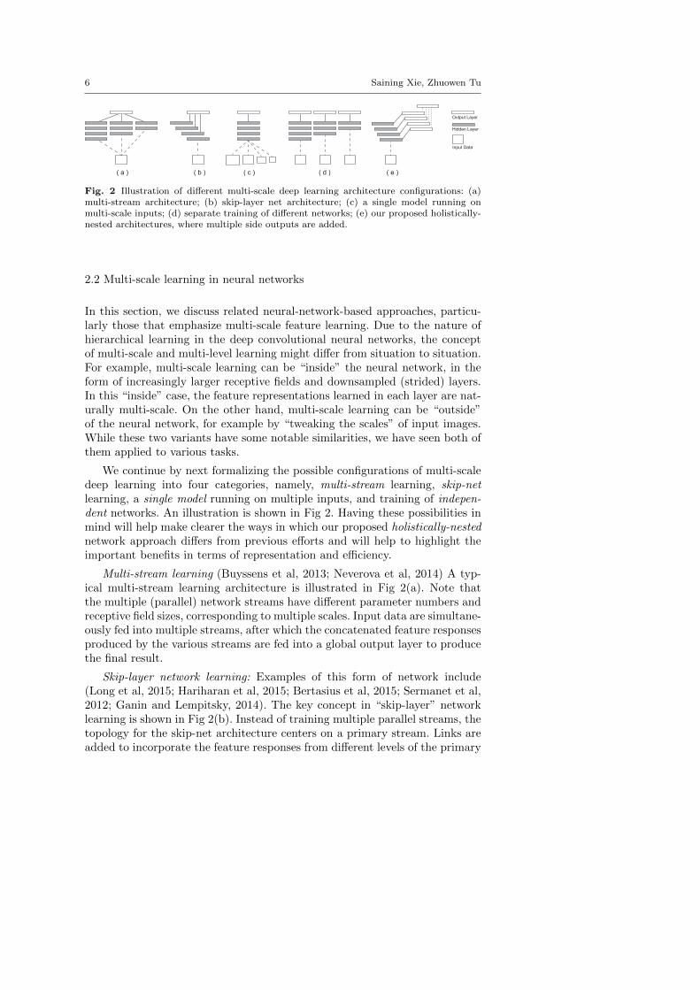
Fig. 2 Illustration of different multi-scale deep learning architecture configurations: (a)multi-stream architecture; (b) skip-layer net architecture; (c) a single model running onmulti-scale inputs; (d) separate training of different networks; (e) our proposed holistically-nested architectures, where multiple side outputs are added.
2.2 Multi-scale learning in neural networks
In this section, we discuss related neural-network-based approaches, particu-larly those that emphasize multi-scale feature learning. Due to the nature ofhierarchical learning in the deep convolutional neural networks, the conceptof multi-scale and multi-level learning might differ from situation to situation.For example, multi-scale learning can be “inside” the neural network, in theform of increasingly larger receptive fields and downsampled (strided) layers.In this “inside” case, the feature representations learned in each layer are nat-urally multi-scale. On the other hand, multi-scale learning can be “outside”of the neural network, for example by “tweaking the scales” of input images.While these two variants have some notable similarities, we have seen both ofthem applied to various tasks.
We continue by next formalizing the possible configurations of multi-scaledeep learning into four categories, namely, multi-stream learning, skip-netlearning, a single model running on multiple inputs, and training of indepen-dent networks. An illustration is shown in Fig 2. Having these possibilities inmind will help make clearer the ways in which our proposed holistically-nestednetwork approach differs from previous efforts and will help to highlight theimportant benefits in terms of representation and efficiency.
Multi-stream learning (Buyssens et al, 2013; Neverova et al, 2014) A typ-ical multi-stream learning architecture is illustrated in Fig 2(a). Note thatthe multiple (parallel) network streams have different parameter numbers andreceptive field sizes, corresponding to multiple scales. Input data are simultane-ously fed into multiple streams, after which the concatenated feature responsesproduced by the various streams are fed into a global output layer to producethe final result.
Skip-layer network learning: Examples of this form of network include(Long et al, 2015; Hariharan et al, 2015; Bertasius et al, 2015; Sermanet et al,2012; Ganin and Lempitsky, 2014). The key concept in “skip-layer” networklearning is shown in Fig 2(b). Instead of training multiple parallel streams, thetopology for the skip-net architecture centers on a primary stream. Links areadded to incorporate the feature responses from different levels of the primary
Holistically-Nested Edge Detection 7
network stream, and these responses are then combined in a shared outputlayer.
A common point in the two settings above is that, in both of the architec-tures, there is only one output loss function with a single prediction produced.However, in edge detection, it is often favorable (and indeed prevalent) toobtain multiple predictions to combine the edge maps together.
Single model on multiple inputs: To get multi-scale predictions, one canalso run a single network (or networks with tied weights) on multiple (scaled)input images, as illustrated in Fig 2(c). This strategy can happen at both thetraining stage (as data augmentation) and at the testing stage (as “ensembletesting”). One notable example is the tied-weight pyramid networks (Farabetet al, 2013). This approach is also common in non-deep-learning based methods(Dollar and Zitnick, 2015). Note that ensemble testing impairs the predictionefficiency of learning systems, especially with deeper models(Bertasius et al,2015; Ganin and Lempitsky, 2014).
Training independent networks: As an extreme variant to Fig 2(a), onemight pursue Fig 2(d), in which multi-scale predictions are made by trainingmultiple independent networks with different depths and different output losslayers. This might be practically challenging to implement as this duplicationwould multiply the amount of resources required for training.
Holistically-nested networks: We list these variants to help clarify thedistinction between existing approaches and our proposed holistically-nestednetwork approach, illustrated in Fig 2(e). There is often significant redun-dancy in existing approaches, in terms of both representation and compu-tational complexity. Our proposed holistically-nested network is a relativelysimple variant that is able to produce predictions from multiple scales. Thearchitecture can be interpreted as a “holistically-nested” version of the “in-dependent networks” approach in Fig 2(d), motivating our choice of name.Our architecture comprises a single-stream deep network with multiple sideoutputs. This architecture resembles several previous works, particularly thedeeply-supervised net(Lee et al, 2015) approach in which the authors showthat hidden layer supervision can improve both optimization and generaliza-tion for image classification tasks. The multiple side outputs also give us theflexibility to add an additional fusion layer if a unified output is desired.
3 Our Approach and Formulation
In this section, we describe in detail our our proposed HED edge detectionsystem and start by introducing the formulation first.
3.1 Formulation
In this section, We give the formulation of HED and discuss in detail thetraining and testing procedure, as well as the network structures of HED.

8 Saining Xie, Zhuowen Tu
3.1.1 Training
We denote our input training data set by S = {(Xn, Yn), n = 1, . . . , N},where sample Xn = {x(n)j , j = 1, . . . , |Xn|} denotes the raw input image and
Yn = {y(n)j , j = 1, . . . , |Xn|}, y(n)j ∈ {0, 1} denotes the corresponding groundtruth binary edge map for image Xn. We subsequently drop the subscriptn for notational simplicity, since we consider each image holistically and in-dependently. Our goal is to have a network that learns features from whichit is possible to produce edge maps approaching the ground truth. For sim-plicity, we denote the collection of all standard network layer parameters asW. Suppose in the network we have M side-output layers. Each side-outputlayer is also associated with a classifier, in which the corresponding weightsare denoted as w = (w(1), . . . ,w(M)). We consider the objective function
Lside(W,w) =
M∑m=1
αm`(m)side(W,w(m)), (1)
where `side denotes the image-level loss function for side-outputs. In our image-to-image training, the loss function is computed over all pixels in a trainingimage X = (xj , j = 1, . . . , |X|) and edge map Y = (yj , j = 1, . . . , |X|), yj ∈{0, 1}. For a typical natural image, the distribution of edge/non-edge pixelsis heavily biased: 90% of the ground truth is non-edge. A cost-sensitive lossfunction is proposed in (Hwang and Liu, 2015), with additional trade-off pa-rameters introduced for biased sampling.
We instead use a simpler strategy to automatically balance the loss betweenpositive/negative classes. We introduce a class-balancing weight β on a per-pixel term basis. Index j is over the image spatial dimensions of image X.Then we use this class-balancing weight as a simple way to offset this imbalancebetween edge and non-edge. Specifically, we define the following class-balancedcross-entropy loss function used in Equation (1)
`(m)side(W,w(m)) = −β
∑j∈Y+
log Pr(yj = 1|X; W,w(m))
−(1− β)∑j∈Y−
log Pr(yj = 0|X; W,w(m)) (2)
where β = |Y−|/|Y | and 1 − β = |Y+|/|Y |. |Y−| and |Y+| denote the edgeand non-edge ground truth label sets, respectively. Pr(yj = 1|X; W,w(m)) =
σ(a(m)j ) ∈ [0, 1] is computed using sigmoid function σ(.) on the activation value
at pixel j. At each side output layer, we then obtain edge map predictions
Y(m)side = σ(A
(m)side), where A
(m)side ≡ {a
(m)j , j = 1, . . . , |Y |} are activations of the
side-output of layer m.To directly utilize side-output predictions, we add a “weighted-fusion” layer
to the network and (simultaneously) learn the fusion weight during training.Our loss function at the fusion layer Lfuse becomes
Lfuse(W,w,h) = Dist(Y, Yfuse) (3)
Holistically-Nested Edge Detection 9
Side-output layer Error Propagation Path
Weighted-fusion layer Error Propagation Pathground truth
Input image X
Side-output 1
Side-output 2
Side-output 3
Side-output 4
Side-output 5
Y
YReceptive Field Size
5 14 40 92 196
ℒ𝑓𝑓𝑓𝑓𝑓𝑓𝑓𝑓ℓ𝑓𝑓𝑠𝑠𝑠𝑠𝑓𝑓
(1)
ℓ𝑓𝑓𝑠𝑠𝑠𝑠𝑓𝑓(3)
ℓ𝑓𝑓𝑠𝑠𝑠𝑠𝑓𝑓(2)
ℓ𝑓𝑓𝑠𝑠𝑠𝑠𝑓𝑓(4)
ℓ𝑓𝑓𝑠𝑠𝑠𝑠𝑓𝑓(5)
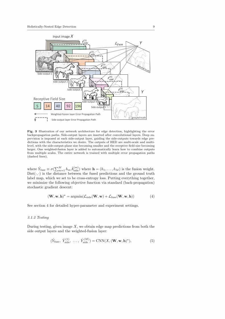
Fig. 3 Illustration of our network architecture for edge detection, highlighting the errorbackpropagation paths. Side-output layers are inserted after convolutional layers. Deep su-pervision is imposed at each side-output layer, guiding the side-outputs towards edge pre-dictions with the characteristics we desire. The outputs of HED are multi-scale and multi-level, with the side-output-plane size becoming smaller and the receptive field size becominglarger. One weighted-fusion layer is added to automatically learn how to combine outputsfrom multiple scales. The entire network is trained with multiple error propagation paths(dashed lines).
where Yfuse ≡ σ(∑M
m=1 hmA(m)side) where h = (h1, . . . , hM ) is the fusion weight.
Dist(·, ·) is the distance between the fused predictions and the ground truthlabel map, which we set to be cross-entropy loss. Putting everything together,we minimize the following objective function via standard (back-propagation)stochastic gradient descent:
(W,w,h)? = argmin(Lside(W,w) + Lfuse(W,w,h)) (4)
See section 4 for detailed hyper-parameter and experiment settings.
3.1.2 Testing
During testing, given image X, we obtain edge map predictions from both theside output layers and the weighted-fusion layer:
(Yfuse, Y(1)side, . . . , Y
(M)side ) = CNN(X, (W,w,h)?), (5)
10 Saining Xie, Zhuowen Tu
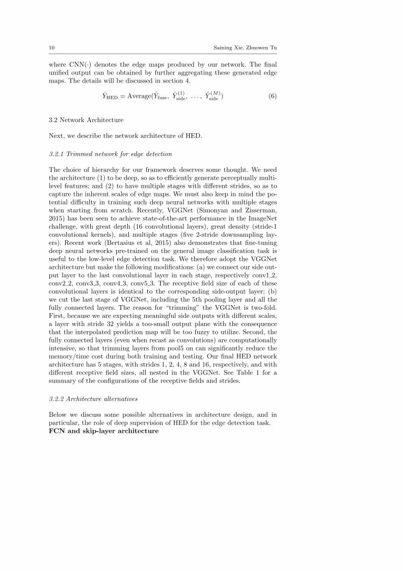
where CNN(·) denotes the edge maps produced by our network. The finalunified output can be obtained by further aggregating these generated edgemaps. The details will be discussed in section 4.
YHED = Average(Yfuse, Y(1)side, . . . , Y
(M)side ) (6)
3.2 Network Architecture
Next, we describe the network architecture of HED.
3.2.1 Trimmed network for edge detection
The choice of hierarchy for our framework deserves some thought. We needthe architecture (1) to be deep, so as to efficiently generate perceptually multi-level features; and (2) to have multiple stages with different strides, so as tocapture the inherent scales of edge maps. We must also keep in mind the po-tential difficulty in training such deep neural networks with multiple stageswhen starting from scratch. Recently, VGGNet (Simonyan and Zisserman,2015) has been seen to achieve state-of-the-art performance in the ImageNetchallenge, with great depth (16 convolutional layers), great density (stride-1convolutional kernels), and multiple stages (five 2-stride downsampling lay-ers). Recent work (Bertasius et al, 2015) also demonstrates that fine-tuningdeep neural networks pre-trained on the general image classification task isuseful to the low-level edge detection task. We therefore adopt the VGGNetarchitecture but make the following modifications: (a) we connect our side out-put layer to the last convolutional layer in each stage, respectively conv1 2,conv2 2, conv3 3, conv4 3, conv5 3. The receptive field size of each of theseconvolutional layers is identical to the corresponding side-output layer; (b)we cut the last stage of VGGNet, including the 5th pooling layer and all thefully connected layers. The reason for “trimming” the VGGNet is two-fold.First, because we are expecting meaningful side outputs with different scales,a layer with stride 32 yields a too-small output plane with the consequencethat the interpolated prediction map will be too fuzzy to utilize. Second, thefully connected layers (even when recast as convolutions) are computationallyintensive, so that trimming layers from pool5 on can significantly reduce thememory/time cost during both training and testing. Our final HED networkarchitecture has 5 stages, with strides 1, 2, 4, 8 and 16, respectively, and withdifferent receptive field sizes, all nested in the VGGNet. See Table 1 for asummary of the configurations of the receptive fields and strides.
3.2.2 Architecture alternatives
Below we discuss some possible alternatives in architecture design, and inparticular, the role of deep supervision of HED for the edge detection task.FCN and skip-layer architecture
Holistically-Nested Edge Detection 11
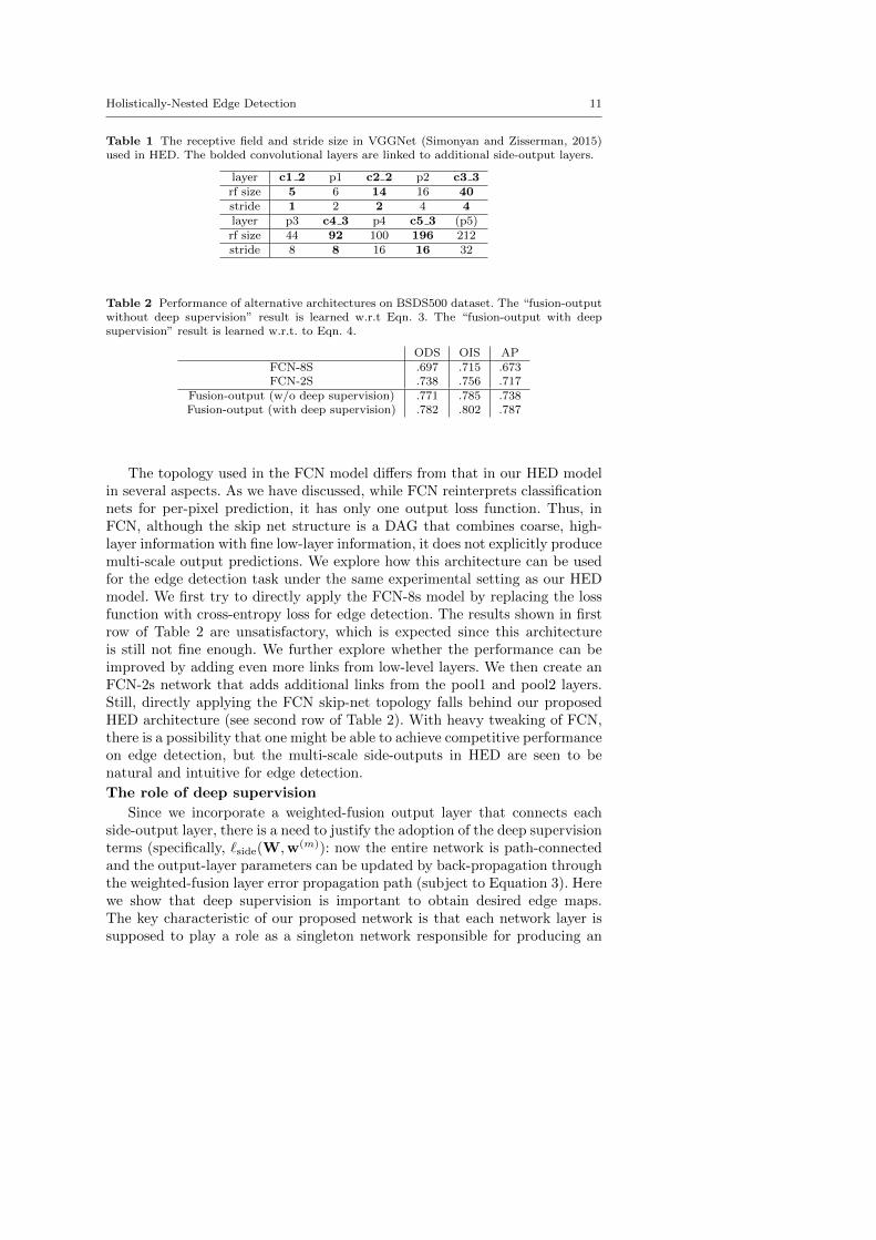
Table 1 The receptive field and stride size in VGGNet (Simonyan and Zisserman, 2015)used in HED. The bolded convolutional layers are linked to additional side-output layers.
layer c1 2 p1 c2 2 p2 c3 3rf size 5 6 14 16 40stride 1 2 2 4 4layer p3 c4 3 p4 c5 3 (p5)rf size 44 92 100 196 212stride 8 8 16 16 32
Table 2 Performance of alternative architectures on BSDS500 dataset. The “fusion-outputwithout deep supervision” result is learned w.r.t Eqn. 3. The “fusion-output with deepsupervision” result is learned w.r.t. to Eqn. 4.
ODS OIS APFCN-8S .697 .715 .673FCN-2S .738 .756 .717
Fusion-output (w/o deep supervision) .771 .785 .738Fusion-output (with deep supervision) .782 .802 .787
The topology used in the FCN model differs from that in our HED modelin several aspects. As we have discussed, while FCN reinterprets classificationnets for per-pixel prediction, it has only one output loss function. Thus, inFCN, although the skip net structure is a DAG that combines coarse, high-layer information with fine low-layer information, it does not explicitly producemulti-scale output predictions. We explore how this architecture can be usedfor the edge detection task under the same experimental setting as our HEDmodel. We first try to directly apply the FCN-8s model by replacing the lossfunction with cross-entropy loss for edge detection. The results shown in firstrow of Table 2 are unsatisfactory, which is expected since this architectureis still not fine enough. We further explore whether the performance can beimproved by adding even more links from low-level layers. We then create anFCN-2s network that adds additional links from the pool1 and pool2 layers.Still, directly applying the FCN skip-net topology falls behind our proposedHED architecture (see second row of Table 2). With heavy tweaking of FCN,there is a possibility that one might be able to achieve competitive performanceon edge detection, but the multi-scale side-outputs in HED are seen to benatural and intuitive for edge detection.
The role of deep supervision
Since we incorporate a weighted-fusion output layer that connects eachside-output layer, there is a need to justify the adoption of the deep supervisionterms (specifically, `side(W,w(m)): now the entire network is path-connectedand the output-layer parameters can be updated by back-propagation throughthe weighted-fusion layer error propagation path (subject to Equation 3). Herewe show that deep supervision is important to obtain desired edge maps.The key characteristic of our proposed network is that each network layer issupposed to play a role as a singleton network responsible for producing an
12 Saining Xie, Zhuowen Tu
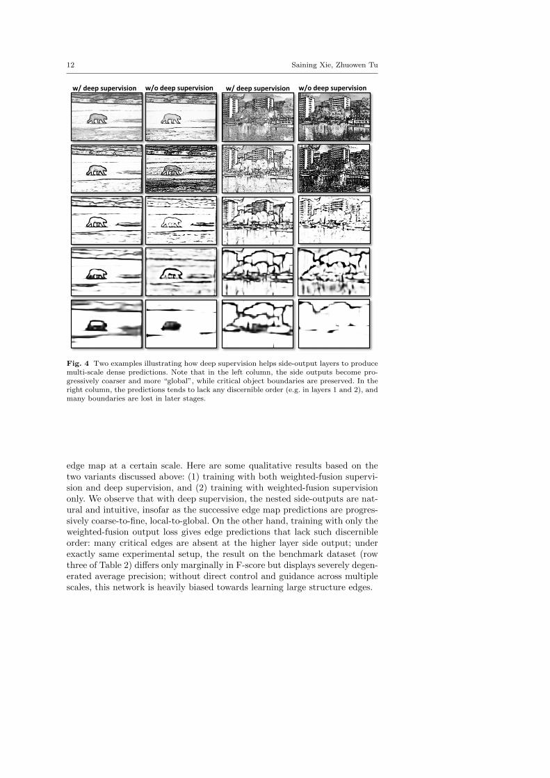
w/o deep supervision w/ deep supervision w/o deep supervision w/ deep supervision
Fig. 4 Two examples illustrating how deep supervision helps side-output layers to producemulti-scale dense predictions. Note that in the left column, the side outputs become pro-gressively coarser and more “global”, while critical object boundaries are preserved. In theright column, the predictions tends to lack any discernible order (e.g. in layers 1 and 2), andmany boundaries are lost in later stages.
edge map at a certain scale. Here are some qualitative results based on thetwo variants discussed above: (1) training with both weighted-fusion supervi-sion and deep supervision, and (2) training with weighted-fusion supervisiononly. We observe that with deep supervision, the nested side-outputs are nat-ural and intuitive, insofar as the successive edge map predictions are progres-sively coarse-to-fine, local-to-global. On the other hand, training with only theweighted-fusion output loss gives edge predictions that lack such discernibleorder: many critical edges are absent at the higher layer side output; underexactly same experimental setup, the result on the benchmark dataset (rowthree of Table 2) differs only marginally in F-score but displays severely degen-erated average precision; without direct control and guidance across multiplescales, this network is heavily biased towards learning large structure edges.
Holistically-Nested Edge Detection 13
4 Experiments
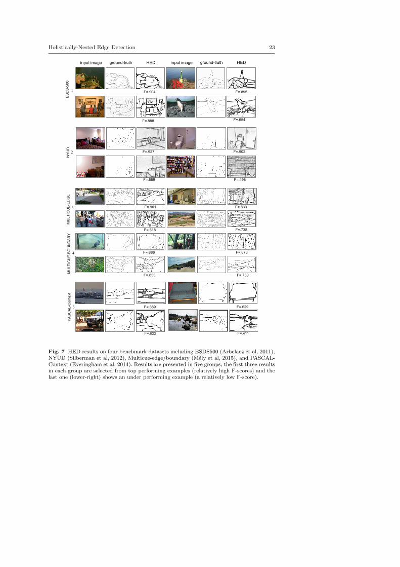
In this section we discuss our detailed implementation and report the perfor-mance of our proposed algorithm. We experiment HED on four benchmarkdatasets including BSDS500 (Arbelaez et al, 2011), NYUD (Silberman et al,2012), Multicue-edge/boundary (Mely et al, 2015) and PASCAL-Context (Ev-eringham et al, 2014). Some qualitative results are shown in Figure 7.
4.1 Implementation
We implement our framework using the publicly available Caffe Library andbuild on top of the publicly available implementations of FCN(Long et al,2015) and DSN(Lee et al, 2015). Thus, relatively little engineering hacking isrequired. In our HED system, the network is fine-tuned from the VGG-16 Netmodel (Simonyan and Zisserman, 2015)Model parameters. In contrast to fine-tuning CNN for image classificationor semantic segmentation, adapting CNN for low-level edge detection requiresspecial care. Even with initialization from a pre-trained model, sparse groundtruth distributions coupled with conventional loss functions lead to difficul-ties in network convergence. Following the strategies outlined in (Dollar andZitnick, 2015), we evaluated various network modification as well as traininghyper-parameters on a validation set. Through experimentation, we choosethe following hyper-parameters: mini-batch size (10), learning rate (1e-6), loss-weight αm for each side-output layer (1), momentum (0.9), nested filter ini-tialization weights (0), fusion layer initialization weights (1/5), weight decay(0.0002), training iterations (10,000; divide learning rate by 10 after 5,000).We found that these hyper-parameters led to the best performance and de-viations in F-score on the validation set tended to be very small. We alsoinvestigated the use of additional nonlinearities by adding an additional layer(with 50 filters and a ReLU) prior to each side-output layer; and that thisdecreased performance. We also observed that nested multi-scale framework isinsensitive to input image scales so, we train on full-resolution images withoutany resizing or cropping. In the experiments that follow, we fix the values ofall hyper-parameters discussed above and concentrate on benefits of specificvariants of HED.Consensus sampling. In our approach, we duplicate the ground truth ateach side-output layer and resize the (downsampled) side output to its origi-nal scale creating a mismatch in the high-level side-outputs. The edge predic-tions are coarse and global, while the ground truth still contains many weakedges that could be considered as noise. This leads to problematic conver-gence behavior, even with the help of a pre-trained model. We observe thatthis mismatch leads to gradients that explode at the high-level side-outputlayers. Therefore, we adjust ground truth labels in the BSDS500 dataset tocombat this issue. Specifically, the ground truth labels are provided by mul-tiple annotators so greater labeler consensus indicates stronger ground truth
14 Saining Xie, Zhuowen Tu
edges. During training, we use majority voting to obtain the positive labels.For example, on BSDS500 dataset, where each image was segmented by fivedifferent subjects on average, we assign a pixel to be positive if and only if itis labeled as positive by at least three annotators. All other labeled pixels arecasted into negatives. This greatly helps convergence in the side-output layers.For low level layers, this consensus approach brings additional regularizationto edge point classification and prevents the network from being distracted byweak edges. Although not fully explored in our paper, a careful handling ofconsensus levels of ground truth edges might lead to further improvement.
Data augmentation. Data augmentation has proven to be a crucial tech-nique in deep networks. We rotate the images to 16 different angles and cropthe largest rectangle in the rotated image; we also flip the image at each an-gle, leading to an augmented training set that is a factor of 32 larger thanthe unaugmented set. After our conference paper (Xie and Tu, 2015), we addadditional augmentation by scaling the training images to 50%, 100%, 150%of its original size. Though holistically-nested networks naturally handle themulti-scale feature learning with its architecture design, we found that thescale augmentation improves the edge detection results from ODS=0.782 toODS=0.790. During testing we operate on an input image at its original size.We also note that “ensemble testing” (making predictions on rotated/flippedimages and averaging the predictions) yields no improvements in F-score, norin average precision.
Different pooling functions. Previous work (Bertasius et al, 2015) suggeststhat different pooling functions can have a major impact on edge detectionresults. We conduct a controlled experiment in which all pooling layers arereplaced by average pooling. We find that using average pooling decrease theperformance to ODS=.741.
In-network bilinear interpolation. Side-output prediction upsampling isimplemented with in-network deconvolutional layers, similar to those in (Longet al, 2015). We fix all the deconvolutional layers to perform linear interpo-lation. Although it was pointed out in (Long et al, 2015) that one can learnarbitrary interpolation functions, we find that learned deconvolutions provideno noticeable improvements in our experiments.
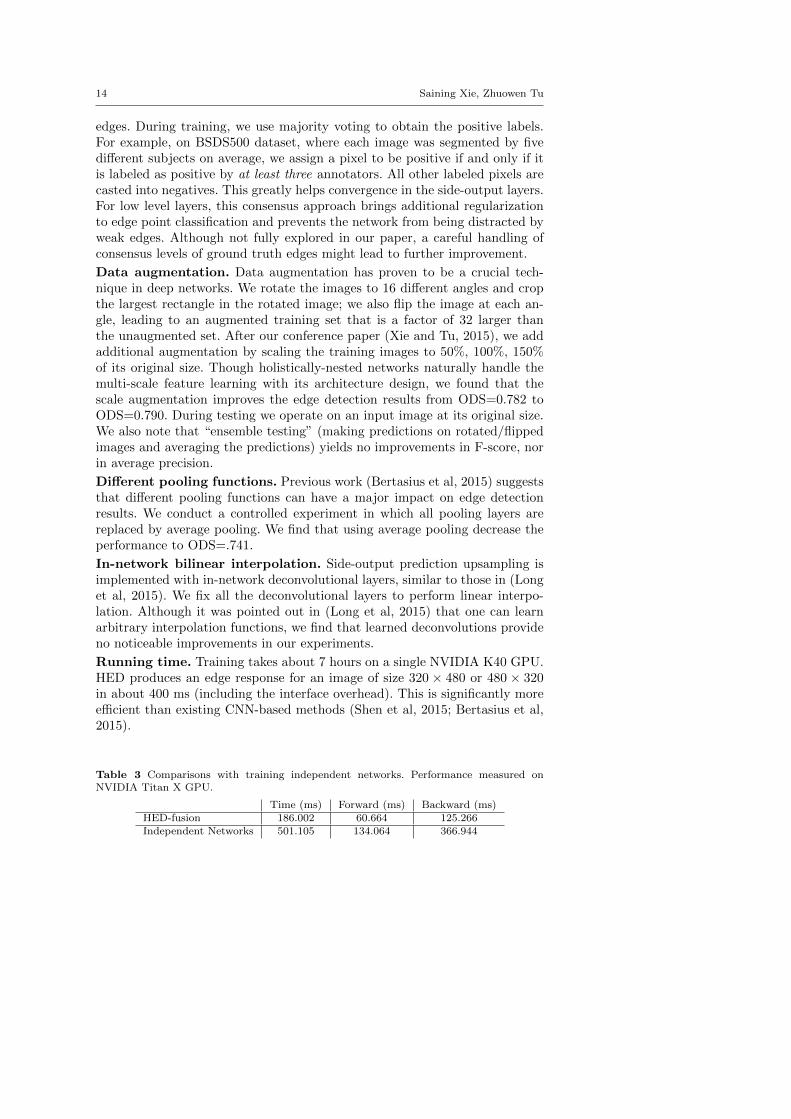
Running time. Training takes about 7 hours on a single NVIDIA K40 GPU.HED produces an edge response for an image of size 320 × 480 or 480 × 320in about 400 ms (including the interface overhead). This is significantly moreefficient than existing CNN-based methods (Shen et al, 2015; Bertasius et al,2015).
Table 3 Comparisons with training independent networks. Performance measured onNVIDIA Titan X GPU.
Time (ms) Forward (ms) Backward (ms)HED-fusion 186.002 60.664 125.266Independent Networks 501.105 134.064 366.944

Holistically-Nested Edge Detection 15
Training independent networks. Our approach builds upon configurationD in Figure 2, however we achieve the same or better performance by us-ing a nested multi-scale model that is also faster and more compact. As aproof-of-concept and sanity check, we train 5 independent networks inducedfrom the five convolutional blocks of VGG-net. Those networks are of differentdepths, where the number of convolutional layers are 2, 4, 7, 10, 13, respec-tively. During test, we average the outputs of these individual networks as thefinal prediction. These independent networks achieve an ODS=0.784 where-asHED achieves an ODS=0.790 under the same experimental conditions. Com-paring the speed of each approach by clocking neural network iteration time,illustrates another advantage of HED over independent networks. Unsurpris-ingly, HED is significantly faster. Table 3 summarizes the forward, backward,and overall iteration time, averaged over 50 iterations. As shown in the table,HED achieves the better ODS score with a 2.7x speed-up compared to thebrute-force ensemble of independent networks.
4.2 BSDS500 dataset
We evaluate HED on the Berkeley Segmentation Dataset and Benchmark(BSDS500) (Arbelaez et al, 2011). BSDS500 is composed of 200 training, 100validation, and 200 testing images where each image is manually annotatedground truth contours. Edge detection accuracy is evaluated using three stan-dard measures: fixed contour threshold (ODS), per-image best threshold (OIS),and average precision (AP). We apply a standard non-maximal suppressiontechnique to our edge maps to obtain thinned edges for evaluation.
First, we report the results of the original HED system (Xie and Tu, 2015)in which an input image is resized to a fixed size of 400× 400. We name thisalgorithm HED (400 × 400). Second, we report improved results of trainingHED by preserving the image aspect ratio and performing additional dataaugmentation. These results are show in Table 5 and Figure 5.Side outputs. To explicitly validate the side outputs, we summarize theresults produced by the individual side-outputs at different scales in Table 4,including different combinations of the multi-scale edge maps. We emphasizehere that all the side-output predictions are obtained in one pass; this enablesus to fully investigate different configurations of combining the outputs atno extra cost. There are several interesting observations from the results: forinstance, combining predictions from multiple scales yields better performance;moreover, all the side-output layers contribute to performance gain, either inF-score or averaged precision. We see this in Table 4, where the side-outputlayer 1 and layer 5 (the lowest and highest layers) achieve similar relativelylow performance. One might conclude that these two side-output layers wouldnot be useful in the averaged results,however, this turns out to false. Theaverage of side-outputs 1-4 achieves ODS=0.760, but incorporating side-output(5) increases performance to ODS=0.774. We find similar phenomenon whenconsidering other ranges. As mentioned above, the predictions obtained using
16 Saining Xie, Zhuowen Tu
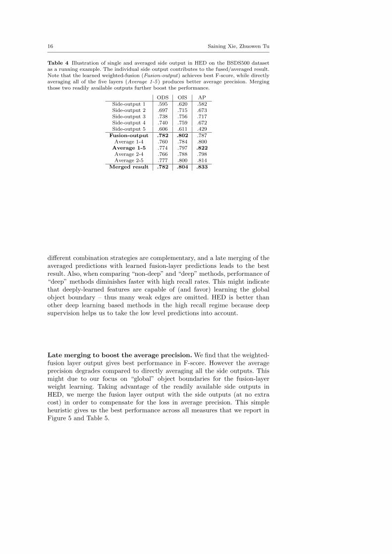
Table 4 Illustration of single and averaged side output in HED on the BSDS500 datasetas a running example. The individual side output contributes to the fused/averaged result.Note that the learned weighted-fusion (Fusion-output) achieves best F-score, while directlyaveraging all of the five layers (Average 1-5 ) produces better average precision. Mergingthose two readily available outputs further boost the performance.
ODS OIS APSide-output 1 .595 .620 .582Side-output 2 .697 .715 .673Side-output 3 .738 .756 .717Side-output 4 .740 .759 .672Side-output 5 .606 .611 .429
Fusion-output .782 .802 .787Average 1-4 .760 .784 .800Average 1-5 .774 .797 .822Average 2-4 .766 .788 .798Average 2-5 .777 .800 .814
Merged result .782 .804 .833
different combination strategies are complementary, and a late merging of theaveraged predictions with learned fusion-layer predictions leads to the bestresult. Also, when comparing “non-deep” and “deep” methods, performance of“deep” methods diminishes faster with high recall rates. This might indicatethat deeply-learned features are capable of (and favor) learning the globalobject boundary – thus many weak edges are omitted. HED is better thanother deep learning based methods in the high recall regime because deepsupervision helps us to take the low level predictions into account.
Late merging to boost the average precision. We find that the weighted-fusion layer output gives best performance in F-score. However the averageprecision degrades compared to directly averaging all the side outputs. Thismight due to our focus on “global” object boundaries for the fusion-layerweight learning. Taking advantage of the readily available side outputs inHED, we merge the fusion layer output with the side outputs (at no extracost) in order to compensate for the loss in average precision. This simpleheuristic gives us the best performance across all measures that we report inFigure 5 and Table 5.
Holistically-Nested Edge Detection 17
0 0.1 0.2 0.3 0.4 0.5 0.6 0.7 0.8 0.9 10
0.1
0.2
0.3
0.4
0.5
0.6
0.7
0.8
0.9
1
Recall
Pre
cisi
on
[F=.790] HED (ours)[F=.788] HED−merge (ours)[F=.756] DeepContour[F=.756] CSCNN[F=.753] DeepEdge[F=.749] OEF[F=.747] SE+multi−ucm[F=.746] SE[F=.739] SCG[F=.727] Sketch Tokens[F=.726] gPb−owt−ucm[F=.723] ISCRA[F=.694] Gb[F=.640] Mean Shift[F=.640] Normalized Cuts[F=.610] Felz−Hutt[F=.600] Canny
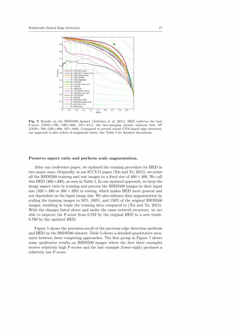
Fig. 5 Results on the BSDS500 dataset (Arbelaez et al, 2011). HED achieves the bestF-score (ODS=.790, OIS=.808, AP=.811), the late-merging variant achieves best AP(ODS=.788, OIS=.808, AP=.840). Compared to several recent CNN-based edge detectors,our approach is also orders of magnitude faster. See Table 5 for detailed discussions.
Preserve aspect ratio and perform scale augmentation.
After our conference paper, we updated the training procedure for HED intwo major ways. Originally, in our ICCV15 paper (Xie and Tu, 2015), we resizeall the BSDS500 training and test images to a fixed size of 400× 400. We callthis HED (400×400), as seen in Table 5. In our updated approach, we keep theimage aspect ratio in training and process the BSDS500 images in their inputsize (320× 480 or 480× 320) in testing, which makes HED more general andnot dependent on the input image size. We also enhance data augmentation byscaling the training images to 50%, 100%, and 150% of the original BSDS500images, resulting in triple the training data compared to (Xie and Tu, 2015).With the changes listed above and under the same network structure, we areable to improve the F-score from 0.782 by the original HED to a new result,0.790 by the updated HED.
Figure 5 shows the precision-recall of the previous edge detection methodsand HED on the BSDS500 dataset; Table 5 shows a detailed quantitative mea-sures between these competing approaches. The first group in Figure 7 showssome qualitative results on BSDS500 images where the first three examplesreceive relatively high F-scores and the last example (lower-right) produces arelatively low F-score.
18 Saining Xie, Zhuowen Tu
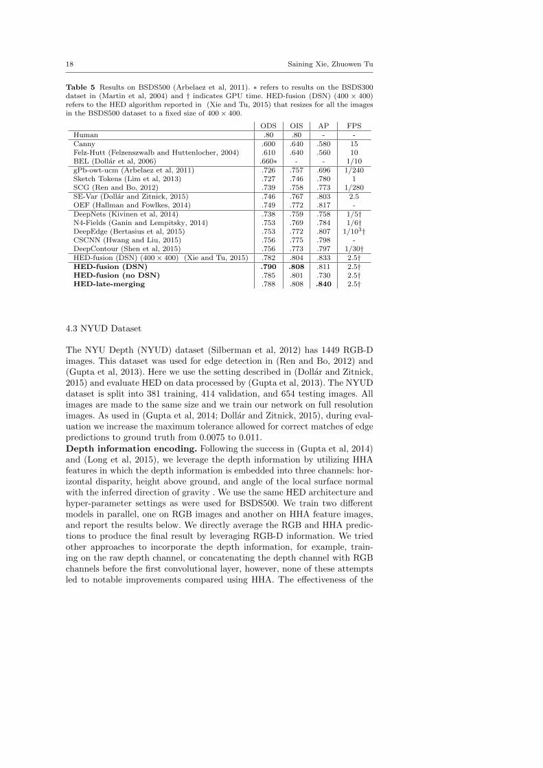
Table 5 Results on BSDS500 (Arbelaez et al, 2011). ∗ refers to results on the BSDS300datset in (Martin et al, 2004) and † indicates GPU time. HED-fusion (DSN) (400 × 400)refers to the HED algorithm reported in (Xie and Tu, 2015) that resizes for all the imagesin the BSDS500 dataset to a fixed size of 400× 400.
ODS OIS AP FPSHuman .80 .80 - -Canny .600 .640 .580 15Felz-Hutt (Felzenszwalb and Huttenlocher, 2004) .610 .640 .560 10BEL (Dollar et al, 2006) .660∗ - - 1/10gPb-owt-ucm (Arbelaez et al, 2011) .726 .757 .696 1/240Sketch Tokens (Lim et al, 2013) .727 .746 .780 1SCG (Ren and Bo, 2012) .739 .758 .773 1/280SE-Var (Dollar and Zitnick, 2015) .746 .767 .803 2.5OEF (Hallman and Fowlkes, 2014) .749 .772 .817 -DeepNets (Kivinen et al, 2014) .738 .759 .758 1/5†N4-Fields (Ganin and Lempitsky, 2014) .753 .769 .784 1/6†DeepEdge (Bertasius et al, 2015) .753 .772 .807 1/103†CSCNN (Hwang and Liu, 2015) .756 .775 .798 -DeepContour (Shen et al, 2015) .756 .773 .797 1/30†HED-fusion (DSN) (400× 400) (Xie and Tu, 2015) .782 .804 .833 2.5†HED-fusion (DSN) .790 .808 .811 2.5†HED-fusion (no DSN) .785 .801 .730 2.5†HED-late-merging .788 .808 .840 2.5†
4.3 NYUD Dataset
The NYU Depth (NYUD) dataset (Silberman et al, 2012) has 1449 RGB-Dimages. This dataset was used for edge detection in (Ren and Bo, 2012) and(Gupta et al, 2013). Here we use the setting described in (Dollar and Zitnick,2015) and evaluate HED on data processed by (Gupta et al, 2013). The NYUDdataset is split into 381 training, 414 validation, and 654 testing images. Allimages are made to the same size and we train our network on full resolutionimages. As used in (Gupta et al, 2014; Dollar and Zitnick, 2015), during eval-uation we increase the maximum tolerance allowed for correct matches of edgepredictions to ground truth from 0.0075 to 0.011.Depth information encoding. Following the success in (Gupta et al, 2014)and (Long et al, 2015), we leverage the depth information by utilizing HHAfeatures in which the depth information is embedded into three channels: hor-izontal disparity, height above ground, and angle of the local surface normalwith the inferred direction of gravity . We use the same HED architecture andhyper-parameter settings as were used for BSDS500. We train two differentmodels in parallel, one on RGB images and another on HHA feature images,and report the results below. We directly average the RGB and HHA predic-tions to produce the final result by leveraging RGB-D information. We triedother approaches to incorporate the depth information, for example, train-ing on the raw depth channel, or concatenating the depth channel with RGBchannels before the first convolutional layer, however, none of these attemptsled to notable improvements compared using HHA. The effectiveness of the
Holistically-Nested Edge Detection 19
0 0.1 0.2 0.3 0.4 0.5 0.6 0.7 0.8 0.9 1
0.1
0.2
0.3
0.4
0.5
0.6
0.7
0.8
0.9
1
Recall
Prec
isio
n
0
[F=.746] HED (ours) [F=.710] SE+NG+ [F=.695] SE[F=.685] gPb+NG[F=.655] Silberman[F=.629] gPb−owt−ucm
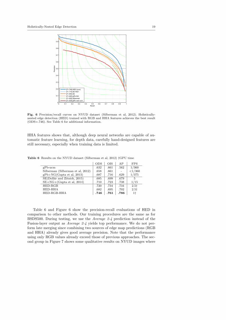
Fig. 6 Precision/recall curves on NYUD dataset (Silberman et al, 2012). Holistically-nested edge detection (HED) trained with RGB and HHA features achieves the best result(ODS=.746). See Table 6 for additional information.
HHA features shows that, although deep neural networks are capable of au-tomatic feature learning, for depth data, carefully hand-designed features arestill necessary, especially when training data is limited.
Table 6 Results on the NYUD dataset (Silberman et al, 2012) †GPU time
ODS OIS AP FPSgPb-ucm .632 .661 .562 1/360Silberman (Silberman et al, 2012) .658 .661 - <1/360gPb+NG(Gupta et al, 2013) .687 .716 .629 1/375SE(Dollar and Zitnick, 2015) .685 .699 .679 5SE+NG+(Gupta et al, 2014) .710 .723 .738 1/15HED-RGB .720 .734 .734 2.5†HED-HHA .682 .695 .702 2.5†HED-RGB-HHA .746 .761 .786 1†
Table 6 and Figure 6 show the precision-recall evaluations of HED incomparison to other methods. Our training procedures are the same as forBSDS500. During testing, we use the Average 2-4 prediction instead of theFusion-layer output as Average 2-4 yields top performance. We do not per-form late merging since combining two sources of edge map predictions (RGBand HHA) already gives good average precision. Note that the performanceusing only RGB values already exceed those of previous approaches. The sec-ond group in Figure 7 shows some qualitative results on NYUD images where
20 Saining Xie, Zhuowen Tu
the first three examples receive relatively high F-scores and the last example(lower-right) produces a relatively low F-score.
4.4 Edges vs. Boundaries: Multicue Dataset
A Multicue edge and boundary dataset, motivated from psychophysics re-search, is recently proposed in (Mely et al, 2015), which consists of 100 shortbinocular video clips of natural scenes captured by a stereo camera. For eachvideo clip (10 frames each), only the last frame of the left sequence is manuallylabeled by human subjects. We call this dataset “Multicue”. There are severalnotable differences between the Multicue dataset and the BSDS500 dataset: (1)Multicue captures complex scenes whereas BSDS500 contains object-centricimages of relatively lower complexity. (2) Each frame in Multicue is of size1, 280 × 720 which is much higher than the 480 × 320 size in BSDS500. (3)Two sets of ground-truth annotations are obtained in Multicue: one account-ing for object boundaries and another focusing on low-level edges. These twoannotations capture different levels of visual perception on the same set ofimages and enable us to study interesting properties of edge detectors that arenot observable when experimenting on the BSDS500 dataset.
In computer vision, “object boundaries” and “edges” are sometimes usedinterchangeably, however under their strict definitions, they refer to visualperception at different stages. Edges are modeled in the early stages of theperception system, e.g. V1 and boundaries correspond to high-level seman-tics that are modeled in the later stages of the perception system, e.g. V4.Note that in this part of the experiment, we follow the definition of “edges”and “boundaries” as defined in (Mely et al, 2015), which is somewhat differ-ent from the “edge” definition in the previous sections when referring to theBSDS500 dataset. One might expect deep learning based edge detectors toexcel when trained to detect (high-level) “boundaries”, and to be less effectivewhen trained to detect (low-level) “edges”. Here, we evaluate the performanceof HED by experimenting on the Multicue dataset.
We keep the same algorithmic and network settings for HED when trainingon BSDS500 and on Multicue. Since the resolution of Multicue is much higher,we randomly crop 500×500 sub-images during training. To further alleviate thescarcity of the labeled data, we augment the training set by random horizontalflipping, rotating (90, 180, and 270 degrees) and scaling (75% and 125%)images and their corresponding ground-truth label maps. We use a learningrate of 1e-6, weight decay 0.0002 and train the model for 2,000 iterations.Following (Mely et al, 2015), we randomly split the dataset into 80 trainingand 20 testing images, and report the averaged score over three independentruns.
Table 7 shows a comparison between HED (trained separately on bound-aries and edges), the method reported in (Mely et al, 2015), and human sub-jects. In (Mely et al, 2015), the authors explicitly study multiple image cues in-cluding intensity, luminance, single/double-opponent color, motion and stereo,

Holistically-Nested Edge Detection 21
Table 7 Edge and boundary detection results on the Multicue dataset (Mely et al, 2015).
ODS OIS APHuman-Boundary .760 (0.017) - -Multicue-Boundary (Mely et al, 2015) .720 (0.014) - -HED-Boundary .814 (0.011) .822 (0.008) .869 (0.015)Human-Edge .750 (0.024) - -Multicue-Edge (Mely et al, 2015) .830 (0.002) - -HED-Edge .851(0.014) .864 (0.011) .890 (0.007)
followed by a fusion procedure to form a region-based mid-level representa-tion, which is then used for training a L2-norm regularized logistic classifier.In “boundary” detection, HED outperforms the method in (Mely et al, 2015)by a large margin of 9.4% absolute improvement. In the task of “edge” detec-tion, HED wins by a relatively smaller gap of 2.1%. These observations areunderstandable and consistent with our hypothesis: for a low-level vision task,features such as color and luminance already provide informative cues; for ahigh-level vision task, multi-scale and multi-level feature learning plays a moreimportant role.
Qualitative results on some Multicue images are shown in the third group(Multicue-edge) and the fourth group (Multicue-boundary) in Figure 7, whereeach group consists of three example images receiving relatively high F-scoresand one example (lower-right) observing a relatively low F-score.
4.5 From Segmentation to Edge Detection: PASCAL-Context Dataset
In this section, we validate HED on another widely used computer visionbenchmark, PASCAL-Context(Mottaghi et al, 2014), which is an extension tothe PASCAL VOC-2010 image segmentation dataset (Everingham et al, 2014),in which 11,530 images are composed of a wide variety of object categoriesbeyond the original 20 object classes in VOC 2010. Recent work (Yang et al,2016; Maninis et al, 2016) shows edge detection results on the original PASCALVOC dataset. We argue that the PASCAL-Context dataset might be moresuitable for our study in this paper, as it is fully labeled, thus has richer andmore diverse edge labelings.
Each image in the PASCAL-Context dataset is associated with a ground-truth label map where each pixel is assigned with a semantic label; generatingedges from image labeling is straight-forward: a pixel is considered a bound-ary pixel if any of its neighbors has a different label. In this experiment, weuse the 60-category version of the dataset. We use the train and validationsplit provided in the original dataset. We train HED on the train split (4998images) and report results on the validation split (5105 images). We keepthe same settings as we use in the BSDS500 experiment, except reducing theinitial learning rate to 1e-7. Similar to the NYUD dataset, due to the incon-sistency of the annotations, we increase the matching tolerance to 0.011 whileevaluating on PASCAL-Context. We show the cross-dataset evaluation results
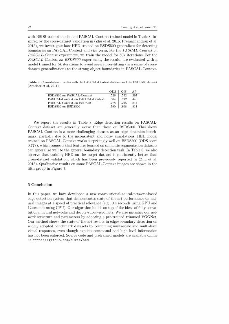
22 Saining Xie, Zhuowen Tu
with BSDS-trained model and PASCAL-Context trained model in Table 8. In-spired by the cross-dataset validation in (Zhu et al, 2015; Premachandran et al,2015), we investigate how HED trained on BSDS500 generalizes for detectingboundaries on PASCAL-Context and vice versa. For the PASCAL-Context onPASCAL-Context experiment, we train the model for 80k iterations. For thePASCAL-Context on BSDS500 experiment, the results are evaluated with amodel trained for 5k iterations to avoid severe over-fitting (in a sense of cross-dataset generalization) to the strong object boundaries in PASCAL-Context.
Table 8 Cross-dataset results with the PASCAL-Context dataset and the BSDS500 dataset(Arbelaez et al, 2011).
ODS OIS APBSDS500 on PASCAL-Context .526 .552 .397PASCAL-Context on PASCAL-Context .584 .592 .443PASCAL-Context on BSDS500 .778 .795 .814BSDS500 on BSDS500 .790 .808 .811
We report the results in Table 8. Edge detection results on PASCAL-Context dataset are generally worse than those on BSDS500. This showsPASCAL-Context is a more challenging dataset as an edge detection bench-mark, partially due to the inconsistent and noisy annotations. HED modeltrained on PASCAL-Context works surprisingly well on BSDS500 (ODS score0.778), which suggests that features learned on semantic segmentation datasetscan generalize well to the general boundary detection task. In Table 8, we alsoobserve that training HED on the target dataset is consistently better thancross-dataset validation, which has been previously reported in (Zhu et al,2015). Qualitative results on some PASCAL-Context images are shown in thefifth group in Figure 7.
5 Conclusion
In this paper, we have developed a new convolutional-neural-network-basededge detection system that demonstrates state-of-the-art performance on nat-ural images at a speed of practical relevance (e.g., 0.4 seconds using GPU and12 seconds using CPU). Our algorithm builds on top of the ideas of fully convo-lutional neural networks and deeply-supervised nets. We also initialize our net-work structure and parameters by adopting a pre-trained trimmed VGGNet.Our method shows the state-of-the-art results in edge/boundary detection onwidely adopted benchmark datasets by combining multi-scale and multi-levelvisual responses, even though explicit contextual and high-level informationhas not been enforced. Source code and pretrained models are available onlineat https://github.com/s9xie/hed.
Holistically-Nested Edge Detection 23
MU
LTIC
UE-
EDG
EM
ULT
ICU
E-BO
UN
DAR
Y
F=.738
F=.901 F=.833
F=.818
F=.886 F=.873
F=.855 F=.750
PASC
AL-C
onte
xt
F=.411
F=.689 F=.629
F=.622
BSD
S-50
0input image ground-truth HED input image ground-truth HED
F=.904 F=.895
F=.888 F=.654
F=.889 F=.498
NYU
D
F=.927 F=.902
1
2
3
4
5
Fig. 7 HED results on four benchmark datasets including BSDS500 (Arbelaez et al, 2011),NYUD (Silberman et al, 2012), Multicue-edge/boundary (Mely et al, 2015), and PASCAL-Context (Everingham et al, 2014). Results are presented in five groups; the first three resultsin each group are selected from top performing examples (relatively high F-scores) and thelast one (lower-right) shows an under performing example (a relatively low F-score).
24 Saining Xie, Zhuowen Tu
Acknowledgment. This work is supported by NSF NSF IIS-1618477IIS-1216528 (IIS-1360566), NSF award IIS-0844566 (IIS-1360568), NSF IIS-1618477,and a Northrop Grumman Contextual Robotics grant. We thank Patrick Gal-lagher and Jameson Merkow for helping improve this manuscript. We alsothank Piotr Dollar and Yin Li for insightful discussions. We are grateful forthe generous donation of the GPUs by NVIDIA.
References
Arbelaez P, Maire M, Fowlkes C, Malik J (2011) Contour detection and hier-archical image segmentation. PAMI 33(5):898–916
Bertasius G, Shi J, Torresani L (2015) Deepedge: A multi-scale bifurcateddeep network for top-down contour detection. In: CVPR
Buyssens P, Elmoataz A, Lezoray O (2013) Multiscale convolutional neuralnetworks for vision–based classification of cells. In: ACCV
Canny J (1986) A computational approach to edge detection. PAMI (6):679–698
Chen LC, Barron JT, Papandreou G, Murphy K, Yuille AL (2015) Seman-tic image segmentation with task-specific edge detection using cnns and adiscriminatively trained domain transform. arXiv preprint arXiv:151103328
Dollar P, Zitnick CL (2015) Fast edge detection using structured forests. PAMIDollar P, Tu Z, Belongie S (2006) Supervised learning of edges and object
boundaries. In: CVPRElder JH, Goldberg RM (2002) Ecological statistics of gestalt laws for the
perceptual organization of contours. Journal of Vision 2(4):5Everingham M, Eslami SA, Van Gool L, Williams CK, Winn J, Zisserman
A (2014) The pascal visual object classes challenge: A retrospective. IJCV111(1):98–136
Farabet C, Couprie C, Najman L, LeCun Y (2013) Learning hierarchical fea-tures for scene labeling. PAMI
Felzenszwalb PF, Huttenlocher DP (2004) Efficient graph-based image seg-mentation. IJCV 59(2):167–181
Ganin Y, Lempitsky V (2014) N4-fields: Neural network nearest neighbor fieldsfor image transforms. arXiv preprint arXiv:14066558
Girshick R, Donahue J, Darrell T, Malik J (2014) Rich feature hierarchies foraccurate object detection and semantic segmentation. In: Computer Visionand Pattern Recognition (CVPR), 2014 IEEE Conference on, IEEE, pp580–587
Gupta S, Arbelaez P, Malik J (2013) Perceptual organization and recognitionof indoor scenes from rgb-d images. In: CVPR
Gupta S, Girshick R, Arbelaez P, Malik J (2014) Learning rich features fromrgb-d images for object detection and segmentation. In: ECCV
Hallman S, Fowlkes CC (2014) Oriented edge forests for boundary detection.arXiv preprint arXiv:14124181

Holistically-Nested Edge Detection 25
Hariharan B, Arbelaez P, Girshick R, Malik J (2015) Hypercolumns for objectsegmentation and fine-grained localization. In: CVPR
Hoiem D, Stein AN, Efros AA, Hebert M (2007) Recovering occlusion bound-aries from a single image. In: ICCV
Hoiem D, Efros AA, Hebert M (2008) Putting objects in perspective. IJCV80(1):3–15
Hou X, Yuille A, Koch C (2013) Boundary detection benchmarking: Beyondf-measures. In: CVPR
Hubel DH, Wiesel TN (1962) Receptive fields, binocular interaction and func-tional architecture in the cat’s visual cortex. The Journal of physiology160(1):106–154
Hwang JJ, Liu TL (2015) Pixel-wise deep learning for contour detection. In:ICLR
Khoreva A, Benenson R, Omran M, Hein M, Schiele B (2016) Weakly super-vised object boundaries. In: CVPR
Kittler J (1983) On the accuracy of the sobel edge detector. Image and VisionComputing 1(1):37–42
Kivinen JJ, Williams CK, Heess N, Technologies D (2014) Visual boundaryprediction: A deep neural prediction network and quality dissection. In:AISTATS
Kokkinos I (2016) Pushing the boundaries of boundary detection using deeplearning. In: ICLR
Konishi S, Yuille AL, Coughlan JM, Zhu SC (2003) Statistical edge detection:Learning and evaluating edge cues. PAMI 25(1):57–74
LeCun Y, Boser B, Denker JS, Henderson D, Howard R, Hubbard W, JackelL (1989) Backpropagation applied to handwritten zip code recognition. In:Neural Computation
Lee CY, Xie S, Gallagher P, Zhang Z, Tu Z (2015) Deeply-supervised nets. In:AISTATS
Li Y, Paluri M, Rehg JM, Dollar P (2016) Unsupervised learning of edges. In:CVPR
Lim JJ, Zitnick CL, Dollar P (2013) Sketch tokens: A learned mid-level rep-resentation for contour and object detection. In: CVPR
Liu C, Yuen J, Torralba A (2011) Nonparametric scene parsing via label trans-fer. PAMI 33(12):2368–2382
Long J, Shelhamer E, Darrell T (2015) Fully convolutional networks for se-mantic segmentation. In: CVPR
Maninis KK, Pont-Tuset J, Arbelaez P, Van Gool L (2016) Convolutionaloriented boundaries. ECCV
Marr D, Hildreth E (1980) Theory of edge detection. Proceedings of the RoyalSociety of London Series B Biological Sciences 207(1167):187–217
Martin DR, Fowlkes CC, Malik J (2004) Learning to detect natural imageboundaries using local brightness, color, and texture cues. PAMI 26(5):530–549
Mely D, Kim J, McGill M, Guo Y, Serre T (2015) A systematic comparisonbetween visual cues for boundary detection. Vision research 120:93–107
26 Saining Xie, Zhuowen Tu
Merkow J, Kriegman D, Marsden A, Tu Z (2016) Dense volume-to-volumevascular boundary detection. In: MICCAI
Mottaghi R, Chen X, Liu X, Cho NG, Lee SW, Fidler S, Urtasun R, Yuille A(2014) The role of context for object detection and semantic segmentationin the wild. In: CVPR
Neverova N, Wolf C, Taylor GW, Nebout F (2014) Multi-scale deep learningfor gesture detection and localization. In: ECCV Workshops
Premachandran V, Bonev B, Yuille AL (2015) Pascal boundaries: A class-agnostic semantic boundary dataset. arXiv preprint arXiv:151107951
Ren X (2008) Multi-scale improves boundary detection in natural images. In:ECCV
Ren X, Bo L (2012) Discriminatively trained sparse code gradients for contourdetection. In: NIPS
Ruderman DL, Bialek W (1994) Statistics of natural images: Scaling in thewoods. Physical review letters 73(6):814
Russakovsky O, Deng J, Su H, Krause J, Satheesh S, Ma S, Huang Z, KarpathyA, Khosla A, Bernstein M, Berg AC, Fei-Fei L (2014) Imagenet large scalevisual recognition challenge. arXiv:1409.0575
Sermanet P, Chintala S, LeCun Y (2012) Convolutional neural networks ap-plied to house numbers digit classification. In: ICPR
Shen W, Wang X, Wang Y, Bai X, Zhang Z (2015) Deepcontour: A deepconvolutional feature learned by positive-sharing loss for contour detectiondraft version. In: CVPR
Shen W, Zhao K, Jiang Y, Wang Y, Zhang Z, Bai X (2016) Object skeletonextraction in natural images by fusing scale-associated deep side outputs.In: CVPR
Silberman N, Hoiem D, Kohli P, Fergus R (2012) Indoor segmentation andsupport inference from rgbd images. In: ECCV
Simonyan K, Zisserman A (2015) Very deep convolutional networks for large-scale image recognition. In: ICLR
Torre V, Poggio TA (1986) On edge detection. PAMI (2):147–163Tu Z (2008) Auto-context and its application to high-level vision tasks. In:
CVPRVan Essen DC, Gallant JL (1994) Neural mechanisms of form and motion
processing in the primate visual system. Neuron 13(1):1–10Witkin AP (1984) Scale-space filtering: A new approach to multi-scale descrip-
tion. In: ICASSPXie S, Tu Z (2015) Holistically-nested edge detection. In: Proceedings of the
IEEE International Conference on Computer Vision, pp 1395–1403Yang J, Price B, Cohen S, Lee H, Yang MH (2016) Object contour detection
with a fully convolutional encoder-decoder network. CVPRYuille AL, Poggio TA (1986) Scaling theorems for zero crossings. PAMI (1):15–
25Zhu Y, Tian Y, Mexatas D, Dollar P (2015) Semantic amodal segmentation.
arXiv preprint arXiv:150901329