Journal of Pure and Applied Algebra 218 (2014) 925–936

Contents lists available at ScienceDirect

Journal of Pure and Applied Algebra

www.elsevier.com/locate/jpaa

Hochschild cohomology of triangular string algebras and itsring structure

María Julia Redondo ∗,1, Lucrecia Román

Instituto de Matemática, Universidad Nacional del Sur, Av. Alem 1253, 8000 Bahía Blanca, Argentina

a r t i c l e i n f o a b s t r a c t

Article history:Received 19 March 2013Received in revised form 29 August 2013Available online 13 November 2013Communicated by C. Kassel

MSC:16E40; 16W99

We compute the Hochschild cohomology groups HH∗(A) in case A is a triangular stringalgebra, and show that its ring structure is trivial.

© 2013 Elsevier B.V. All rights reserved.

1. Introduction

Let A be an associative, finite dimensional algebra over an algebraically closed field k. It is well known that there existsa finite quiver Q such that A is Morita equivalent to kQ /I , where kQ is the path algebra of Q and I is an admissibletwo-sided ideal of kQ .

A finite dimensional algebra is called biserial if the radical of every projective indecomposable module is the sum of twouniserial modules whose intersection is simple or zero, see [11]. These algebras have been studied by several authors andfrom different points of view since there are a lot of natural examples of algebras which turn out to be of this kind.

The representation theory of these algebras was first studied by Gel’fand and Ponomarev in [12]: they have provided themethods in order to classify all their indecomposable representations. This classification shows that special biserial algebrasare always tame, see [21], and tameness of arbitrary biserial algebras was established in [10]. They are an important classof algebras whose representation theory has been very well described, see [2,6].

The subclass of special biserial algebras was first studied by Skowronski and Waschbüsch in [19] where they character-ize the biserial algebras of finite representation type. A classification of the special biserial algebras which are minimalrepresentation-infinite has been given by Ringel in [17].

An algebra is called a string algebra if it is Morita equivalent to a monomial special biserial algebra.The purpose of this paper is to study the Hochschild cohomology groups of a string algebra A and describe its ring

structure.Since A is an algebra over a field k, the Hochschild cohomology groups HHi(A, M) with coefficients in an A-bimodule M

can be identified with the groups ExtiA−A(A, M). In particular, if M is the A-bimodule A, we simple write HHi(A).

Even though the computation of the Hochschild cohomology groups HHi(A) is rather complicated, some approaches havebeen successful when the algebra A is given by a quiver with relations. For instance, explicit formula for the dimensionsof HHi(A) in terms of those combinatorial data have been found in [4,7–9,15,16]. In particular, Hochschild cohomology ofspecial biserial algebras has been considered in [5,20].

* Corresponding author.E-mail addresses: mredondo@criba.edu.ar (M.J. Redondo), lroman@uns.edu.ar (L. Román).

1 The first author is a researcher from CONICET, Argentina. This work has been supported by the project PICT 2011-1510, ANPCyT.

0022-4049/$ – see front matter © 2013 Elsevier B.V. All rights reserved.http://dx.doi.org/10.1016/j.jpaa.2013.10.010

926 M.J. Redondo, L. Román / Journal of Pure and Applied Algebra 218 (2014) 925–936

In the particular case of monomial algebras, that is, algebras A = K Q /I where I can be chosen as generated by paths,one has a detailed description of a minimal resolution of the A-bimodule A, see [3]. In general, the computation of theHochschild cohomology groups using this resolution may lead to hard combinatoric computations. However, for string alge-bras the resolution, and the complex associated, are easier to handle.

The paper is organized as follows. In Section 2 we introduce all the necessary terminology. In Section 3 we recall theresolution given by Bardzell for monomial algebras in [3]. In Section 4 we present all the computations that lead us toTheorem 4.3 where we present the dimension of all the Hochschild cohomology groups of triangular string algebras. InSection 5 we describe the ring structure of the Hochschild cohomology of triangular string algebras.

2. Preliminaries

2.1. Quivers and relations

Let Q be a finite quiver with a set of vertices Q 0, a set of arrows Q 1 and s, t : Q 1 → Q 0 be the maps associating to eacharrow α its source s(α) and its target t(α). A path w of length l is a sequence of l arrows α1 . . . αl such that t(αi) = s(αi+1).We denote by |w| the length of the path w . We put s(w) = s(α1) and t(w) = t(αl). For any vertex x we consider ex thetrivial path of length zero and we put s(ex) = t(ex) = x. An oriented cycle is a non-trivial path w such that s(w) = t(w). IfQ has no oriented cycles, then A is said a triangular algebra.

We say that a path w divides a path u if u = L(w)w R(w), where L(w) and R(w) are not simultaneously paths of lengthzero.

The path algebra kQ is the k-vector space with basis the set of paths in Q ; the product on the basis elements is givenby the concatenation of the sequences of arrows of the paths w and w ′ if they form a path (namely, if t(w) = s(w ′)) andzero otherwise. Vertices form a complete set of orthogonal idempotents. Let F be the two-sided ideal of kQ generated bythe arrows of Q . A two-sided ideal I is said to be admissible if there exists an integer m � 2 such that F m ⊆ I ⊆ F 2. Thepair (Q , I) is called a bound quiver.

It is well known that if A is a basic, connected, finite dimensional algebra over an algebraically closed field k, then thereexists a unique finite quiver Q and a surjective morphism of k-algebras ν : kQ → A, which is not unique in general, withIν = Kerν admissible. The pair (Q , Iν) is called a presentation of A. The elements in I are called relations, kQ /I is said amonomial algebra if the ideal I is generated by paths, and a relation is called quadratic if it is a path of length two.

2.2. String algebras

Recall from [19] that a bound quiver (Q , I) is special biserial if it satisfies the following conditions:

(S1) Each vertex in Q is the source of at most two arrows and the target of at most two arrows;(S2) For an arrow α in Q there is at most one arrow β and at most one arrow γ such that αβ /∈ I and γα /∈ I .

If the ideal I is generated by paths, the bound quiver (Q , I) is string.

An algebra is called special biserial (or string) if it is Morita equivalent to a path algebra kQ /I with (Q , I) a specialbiserial bound quiver (or a string bound quiver, respectively).

Since Hochschild cohomology is invariant under Morita equivalence, whenever we deal with a string algebra A we willassume that it is given by a string presentation A = kQ /I with I satisfying the previous conditions. We also assume thatthe ideal I is generated by paths of minimal length, and we fix a minimal set R of paths, of minimal length, that generatethe ideal I . Moreover, we fix a set P of paths in Q such that the set {γ + I, γ ∈P} is a basis of A = kQ /I .

3. Bardzell’s resolution

We recall that the Hochschild cohomology groups HHi(A) of an algebra A are the groups ExtiA−A(A, A). Since string al-

gebras are monomial algebras, their Hochschild cohomology groups can be computed using a convenient minimal projectiveresolution of A as A-bimodule given in [3].

In order to describe this minimal resolution, we need some definitions and notations.Recall that we have fix a minimal set R of paths, of minimal length, that generate the ideal I . It is clear that no divisor

of an element in R can belong to R.The n-concatenations are elements defined inductively as follows: given any directed path T in Q , consider the set of

vertices that are starting and ending points of arrows belonging to T , and consider the natural order < in this set. Let R(T )

be the set of paths in R that are contained in the directed path T . Take p1 ∈R(T ) and consider the set

L1 = {p ∈ R(T ): s(p1) < s(p) < t(p1)

}.

If L1 �= ∅, let p2 be such that s(p2) is minimal with respect to all p ∈ L1. Now assume that p1, p2, . . . , p j have beenconstructed. Let

M.J. Redondo, L. Román / Journal of Pure and Applied Algebra 218 (2014) 925–936 927

L j+1 = {p ∈ R(T ): t(p j−1) � s(p) < t(p j)

}.

If L j+1 �= ∅, let p j+1 be such that s(p j+1) is minimal with respect to all p ∈ L j+1. Thus (p1, . . . , pn−1) is an n-concatenationand we denote by w(p1, . . . , pn−1) the path from s(p1) to t(pn−1) along the directed path T , and we call it the support ofthe concatenation.

These concatenations can be pictured as follows:

p1

p2

p3

p4

p5

· · ·Let AP0 = Q 0, AP1 = Q 1 and APn the set of supports of n-concatenations.

The construction of the sets APn can also be done dually. Given any directed path T in Q take q1 ∈ R(T ) and considerthe set

Lop1 = {

q ∈ R(T ): s(q1) < t(q) < t(q1)}.

If Lop1 �= ∅, let q2 be such that t(q2) is maximal with respect to all q ∈ Lop

1 . Now assume that q1,q2, . . . ,q j have beenconstructed. Let

Lopj+1 = {

q ∈ R(T ): s(q j) < t(q)� s(q j−1)}.

If Lopj+1 �= ∅, let q j+1 be such that t(q j+1) is maximal with respect to all q ∈ Lop

j+1. Thus (qn−1, . . . ,q1) is an n-op-concatena-tion, we denote by wop(qn−1, . . . ,q1) the path from s(qn−1) to t(q1) along the directed path T , we call it the support of theconcatenation and we denote by APop

n the set of supports of n-op-concatenations constructed in this dual way. Moreover,we denote wop(qn−1, . . . ,q1) = wop(q1, . . . ,qn−1).

For any w ∈ APn define Sub(w) = {w ′ ∈ APn−1: w ′ divides w}.

Example 1. Consider the following relations contained in a directed path T :

p1

p2

p3

p4

p5

p6

p7

Then w = w(p1, p2, p4, p5, p7) is a 6-concatenation, w = wop(p1, p3, p4, p6, p7) and

Sub(w) = {w(p1, p2, p4, p5), w(p2, p3, p5, p6), w(p3, p4, p6, p7)

}.

Lemma 3.1. (See [3, Lemma 3.1].) If n � 2 then APn = APopn .

The previous lemma says that for any n-concatenation (p1, . . . , pn−1) there exists a unique n-op-concatenation(q1, . . . ,qn−1) such that w(p1, . . . , pn−1) = wop(q1, . . . ,qn−1). We want to remark some facts in this construction thatwill be used later. First observe that w(p1) = wop(p1) and w(p1, p2) = wop(p1, p2). Assume that n > 3. It is clear thatqn−1 = pn−1 since they are relations in R contained in the same path and sharing target. When we look for qn−2 we canobserve that the maximality of its target implies that t(pn−2) � t(qn−2). Since elements in R are paths of minimal length,s(pn−2) � s(qn−2). Now t(qn−2) < t(qn−1) = t(pn−1) says that qn−2 �= pn−1 and the minimality of the starting point of pn−1says that s(qn−2) < t(pn−3). Then

s(pn−2)� s(qn−2) < t(pn−3) and t(pn−2) � t

(qn−2) < t(pn−1).

Since s(qn−2) < t(pn−3) � s(pn−1) = s(qn−1) we can continue this procedure in order to prove that, for j = 2,3, . . . ,n − 2,the element qn− j is such that

s(pn− j) � s(qn− j) < t(pn− j−1), t(pn− j) � t

(qn− j) < t(pn− j+1)

and

s(qn− j) < t(pn− j−1) � s(pn− j+1) � s

(qn− j+1).

Finally the minimality of the source of p2 and the inequality t(p1)� t(q1) < t(p2) shows that q1 = p1.

Lemma 3.2. If n,m � 0, n + m � 2 then any w(p1, . . . , pn+m−1) ∈ APn+m can be written in a unique way as

w(p1, . . . , pn+m−1) = (n)w u w(m)

with (n)w = w(p1, . . . , pn−1) ∈ APn, w(m) = wop(qn+1, . . . ,qn+m−1) ∈ APopm and u a path in Q . Moreover, pn = a u b and qn = a′ u b′

with a,a′,b,b′ non-trivial paths, and hence u ∈P .

928 M.J. Redondo, L. Román / Journal of Pure and Applied Algebra 218 (2014) 925–936

Proof. From Lemma 3.1 we know that w(p1, . . . , pn+m−1) = wop(q1, . . . ,qn+m−1). It is clear that w(p1, . . . , pn−1) ∈ APn andwop(qn+1, . . . ,qn+m−1) ∈ APop

m . In order to prove the existence of a path u we just have to observe that the constructionexplained after the previous lemma and the definition of concatenations imply that

t(pn−1)� t(qn−1) � s

(qn+1).

Finally, the relation of u with pn and qn follows from the inequalities

s(pn) < t(pn−1) � s(qn+1) < t(pn) and s

(qn) < t(pn−1) � s

(qn+1) < t

(qn). �

Now we want to study the sets Sub(w) in some particular cases. Observe that for any w ∈ APn , ψ1 = wop(q2, . . . ,qn−1)

and ψ2 = w(p1, . . . , pn−2) belong to Sub(w) and w = L(ψ1)ψ1 = ψ2 R(ψ2).

Lemma 3.3. If w = w(p1, . . . , pn−1) ∈ APn is such that pi has length two for some i with 1 � i � n − 1, then |Sub(w)| = 2.

Proof. Assume that pi = αβ . If i = 1, then any (n − 1)-concatenation different from (p1, . . . , pn−2) and corresponding toan element in Sub(w) must correspond to a divisor of w(p2, . . . , pn−1), hence it is equal to (p2, . . . , pn−1). The proof fori = n − 1 is similar. If 1 < i < n − 1 and w ∈ Sub(w) then w also contains the quadratic relation pi and by the previouslemma we have that

w = (i)w w(n−i), w = ( j) w w(n−1− j)

with t((i) w) = t(( j) w) and s(w(n−i)) = s(w(n−1− j)). Then w is (i) w w1 or w2 w(n−i) , where w1 is the unique element inSub(w(n−i)) sharing source with w(n−i) and w2 is the unique element in Sub((i) w) sharing target with (i)w . �Lemma 3.4. If w = w(p1, . . . , pn−1) = wop(q1, . . . ,qn−1) and qm has length two for some m such that 1 < m < n then qm = pm

and qm−1 = pm−1 .

Proof. Let qm = αβ . In the construction explained after Lemma 3.1 we have seen that

s(qm)

< t(pm−1) � t(qm−1).

Now s(qm) = s(α) and t(qm−1) = t(α), so t(pm−1) = t(qm−1) and hence pm−1 = qm−1. Analogously,

s(qm+1) < t(pm) � t

(qm)

,

s(qm+1) = s(β) and t(qm) = t(β), so t(pm) = t(qm) and hence pm = qm . �In some results that will be shown in the following sections, we will need a description of right divisors of paths of the

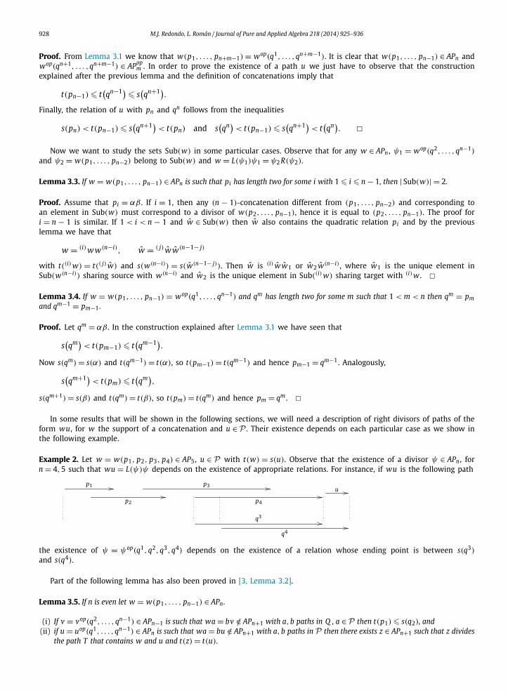
form wu, for w the support of a concatenation and u ∈ P . Their existence depends on each particular case as we show inthe following example.

Example 2. Let w = w(p1, p2, p3, p4) ∈ AP5, u ∈ P with t(w) = s(u). Observe that the existence of a divisor ψ ∈ APn , forn = 4,5 such that wu = L(ψ)ψ depends on the existence of appropriate relations. For instance, if wu is the following path

p1

p2

p3

p4

u

q3

q4

the existence of ψ = ψop(q1,q2,q3,q4) depends on the existence of a relation whose ending point is between s(q3)

and s(q4).

Part of the following lemma has also been proved in [3, Lemma 3.2].

Lemma 3.5. If n is even let w = w(p1, . . . , pn−1) ∈ APn.

(i) If v = vop(q2, . . . ,qn−1) ∈ APn−1 is such that wa = bv /∈ APn+1 with a,b paths in Q , a ∈P then t(p1) � s(q2), and(ii) if u = uop(q1, . . . ,qn−1) ∈ APn is such that wa = bu /∈ APn+1 with a,b paths in P then there exists z ∈ APn+1 such that z divides

the path T that contains w and u and t(z) = t(u).

M.J. Redondo, L. Román / Journal of Pure and Applied Algebra 218 (2014) 925–936 929

Proof. (i) The assumption a ∈ P implies that s(pn−1) < s(qn−1) < t(pn−1), and moreover s(pn−1) < s(qn−1) < t(pn−2) sinceotherwise wa ∈ APn+1 because qn−1 would belong to the set considered in order to choose pn . Now qn−2 = pn−1 ort(pn−1) < t(qn−2), and hence

s(pn−1) < s(qn−2) < s

(qn−1).

Now qn−3 is such that s(pn−3) < s(qn−3) < s(qn−1). The minimality of s(pn−2) says that s(pn−3) < s(qn−3) < t(pn−4). An in-ductive procedure shows that

s(pn−2 j+1) < s(qn−2 j+1) < t(pn−2 j) and qn−2 j = pn−2 j+1 or t(pn−2 j+1) < t

(qn−2 j).

Hence

s(pn−2 j+1) < s(qn−2 j) < s

(qn−2 j+1)

for any j such that 1 � 2 j − 1,2 j � n − 1. In particular, since n is even we have that

q2 = p3 or s(p3) < s(q2) < s

(q3)

and hence t(p1) � s(q2).(ii) In order to prove the existence of z we have to show that there exists q0 ∈ R(T ) such that z = zop(q0,q1, . . . ,qn−1)

belongs to APn+1, that is, we have to see that the set {q ∈ R(T ): s(q1) < t(q) � s(q2)} is not empty. Suppose it is empty.The assumption b ∈P implies that s(q2) < t(p1), a contradiction from (i). �Lemma 3.6. (See [3, Lemma 3.3].) If m � 1 and w ∈ AP2m+1 then |Sub(w)| = 2.

Now we are ready to describe the minimal resolution constructed by Bardzell in [3]:

· · · −→ A ⊗ kAPn ⊗ Adn−→ A ⊗ kAPn−1 ⊗ A −→ · · · −→ A ⊗ kAP0 ⊗ A

μ−→ A −→ 0

where kAP0 = kQ 0, kAP1 = kQ 1 and kAPn is the vector space generated by the set of supports of n-concatenations and alltensor products are taken over E = kQ 0, the subalgebra of A generated by the vertices.

In order to define the A–A-maps

dn : A ⊗ kAPn ⊗ A → A ⊗ kAPn−1 ⊗ A

we need the following notations: if m � 1, for any w ∈ AP2m+1 we have that Sub(w) = {ψ1,ψ2} where w = L(ψ1)ψ1 =ψ2 R(ψ2); and for any w ∈ AP2m and ψ ∈ Sub(w) we denote w = L(ψ)ψ R(ψ). Then

μ(1 ⊗ ei ⊗ 1) = ei,

d1(1 ⊗ α ⊗ 1) = α ⊗ et(α) ⊗ 1 − 1 ⊗ es(α) ⊗ α,

d2m(1 ⊗ w ⊗ 1) =∑

ψ∈Sub(w)

L(ψ) ⊗ ψ ⊗ R(ψ),

d2m+1(1 ⊗ w ⊗ 1) = L(ψ1) ⊗ ψ1 ⊗ 1 − 1 ⊗ ψ2 ⊗ R(ψ2).

The E–A bilinear map c : A ⊗ kAPn−1 ⊗ A → A ⊗ kAPn ⊗ A defined by

c(a ⊗ ψ ⊗ 1) =∑

w∈APnL(w)w R(w)=aψ

L(w) ⊗ w ⊗ R(w)

is a contracting homotopy, see [18, Theorem 1] for more details.

4. Hochschild cohomology

In this section we compute the dimension of all the Hochschild cohomology groups of triangular string algebras.The Hochschild complex, obtained by applying HomA−A(−, A) to the Hochschild resolution we described in the previous

section and using the isomorphisms

HomA−A(A ⊗ kAPn⊗, A) HomE−E(kAPn, A)

is

0 −→ HomE−E(kAP0, A)F1−→ HomE−E(kAP1, A)

F2−→ HomE−E(kAP2, A) · · ·

930 M.J. Redondo, L. Román / Journal of Pure and Applied Algebra 218 (2014) 925–936

where

F1( f )(α) = α f (et(α)) − f (es(α))α,

F2m( f )(w) =∑

ψ∈Sub(w)

L(ψ) f (ψ)R(ψ),

F2m+1( f )(w) = L(ψ1) f (ψ1) − f (ψ2)R(ψ2).

In order to compute its cohomology, we need a manageable description of this complex: we will describe explicit basis ofthese k-vector spaces and study the behavior of the maps between them in order to get information about kernels andimages.

Recall that we have fixed a set P of paths in Q such that the set {γ + I: γ ∈P} is a basis of A = kQ /I . For any subsetX of paths in Q , we denote (X//P) the set of pairs (ρ,γ ) ∈ X ×P such that ρ,γ are parallel paths in Q , that is

(X//P) = {(ρ,γ ) ∈ X ×P: s(ρ) = s(γ ), t(ρ) = t(γ )

}.

Observe that the k-vector spaces HomE−E (kAPn, A) and k(APn//P) are isomorphic, and from now on we will identify ele-ments (ρ,γ ) ∈ (APn//P) with basis elements f(ρ,γ ) in HomE−E (kAPn, A) defined by

f(ρ,γ )(w) ={

γ if w = ρ,

0 otherwise.

Now we will introduce several subsets of (APn//P) in order to get a nice description of the kernel and the image of Fn . Forn = 0 we have that (AP0//P) = (Q 0, Q 0). For n = 1, (AP1//P) = (Q 1//P), and we consider the following partition

(Q 1//P) = (1,1)1 ∪ (0,0)1

where

(1,1)1 = {(α,α): α ∈ Q 1

},

(0,0)1 = {(α,γ ) ∈ (Q 1//P): α �= γ

}.

For any n � 2 let

(0,0)n = {(ρ,γ ) ∈ (APn//P): ρ = α1ρα2 and γ /∈ α1kQ ∪ kQ α2

},

(1,0)n = {(ρ,γ ) ∈ (APn//P): ρ = α1ρα2 and γ ∈ α1kQ , γ /∈ kQ α2

},

(0,1)n = {(ρ,γ ) ∈ (APn//P): ρ = α1ρα2 and γ /∈ α1kQ , γ ∈ kQ α2

},

(1,1)n = {(ρ,γ ) ∈ (APn//P): ρ = α1ρα2 and γ ∈ α1kQ α2

}.

Remark 1.

(1) These subsets are a partition of (APn//P).(2) Any (ρ,γ ) ∈ (APn//P) verifies that ρ and γ have at most one common first arrow and at most one common last

arrow: if ρ = α1 . . . αsβρ and γ = α1 . . . αsδγ , with β, δ different arrows, then αsβ ∈ I . Since α1 . . . αs is a factor of γ ,and γ belongs to P , then α1 . . . αs /∈ I . But the n-concatenation associated to ρ must start with a relation in R(T ), sos = 1, this concatenation starts with the relation α1β and the second relation of this concatenation starts in s(β).

(3) If (ρ,γ ) ∈ (1,0)n , ρ = α1ρ, γ = α1γ then ρ ∈ APn−1 and (ρ, γ ) ∈ (0,0)n−1. The same construction holds in (0,1)n .Finally, if (ρ,γ ) ∈ (1,1)n , ρ = α1ρα2, γ = α1γ α2 then ρ ∈ APn−2 and (ρ, γ ) ∈ (0,0)n−2.

(4) If (ρ,γ ) ∈ (AP2//P) = (R//P), we have already seen that ρ and γ have at most one common first arrow and atmost one common last arrow. Assume that ρ = α1α2ρ , γ = α1βγ . Since A is a string algebra and γ /∈ I we have thatα1α2 ∈ I and hence ρ = α1α2. Since we are dealing with triangular algebras, we also have that ρ and γ cannot havesimultaneously one common first arrow and one common last arrow. Then

(1,1)2 = ∅,

(1,0)2 = {(ρ,γ ) ∈ (R,P): ρ = α1α2, γ ∈ α1kQ , γ /∈ kQ α2

},

(0,1)2 = {(ρ,γ ) ∈ (R,P): ρ = α1α2, γ /∈ α1kQ , γ ∈ kQ α2

}.

We also have to distinguish elements inside each of the previous sets taking into account the following definitions:

+(X//P) = {(ρ,γ ) ∈ (X//P): Q 1γ �⊂ I

},

−(X//P) = {(ρ,γ ) ∈ (X//P): Q 1γ ⊂ I

}.

M.J. Redondo, L. Román / Journal of Pure and Applied Algebra 218 (2014) 925–936 931

In an analogous way we define (X//P)+ , (X//P)− , +(X//P)+ = +(X//P) ∩ (X//P)+ and so on. Finally we define

(1,0)−−n = {

(ρ,γ ) ∈ (1,0)−n : ρ = α1ρα2, γ = α1γ , γ Q 1 ⊂ I},

(1,0)−+n = {

(ρ,γ ) ∈ (1,0)−n : ρ = α1ρα2, γ = α1γ , γ Q 1 �⊂ I},

−−(0,1)n = {(ρ,γ ) ∈ −(0,1)n: ρ = α1ρα2, γ = γ α2, Q 1γ ⊂ I

},

+−(0,1)n = {(ρ,γ ) ∈ −(0,1)n: ρ = α1ρα2, γ = γ α2, Q 1γ �⊂ I

}.

Now we will describe the morphisms Fn restricted to the subsets we have just defined.

Lemma 4.1. For any n � 2 we have

(a) −(0,0)−n−1 ∪ (1,0)−n−1 ∪ −(0,1)n−1 ∪ (1,1)n−1 ⊂ Ker Fn;(b) the function Fn induces a bijection from −(0,0)+n−1 to −−(0,1)n;(c) the function Fn induces a bijection from +(0,0)−n−1 to (1,0)−−

n ;(d) there exist bijections φm : (1,0)+m → +(0,1)m and ψm : (1,0)−+

m → +−(0,1)m such that

(id + (−1)n−1φn−1

)((1,0)+n−1

) ⊂ Ker Fn,

(−1)n Fn((1,0)+n−1

) = (1,1)n

and

Fn(+(0,0)+n−1

) = (id + (−1)nφn

)((1,0)+n

) ∪ (id + (−1)nψn

)((1,0)−+

n

).

Proof. (a) In order to check that (ρ,γ ) belongs to Ker Fn we have to prove that for any w ∈ APn such that ρ divides w ,that is, w = L(ρ)ρR(ρ) and |L(ρ)| + |R(ρ)| > 0, then L(ρ)γ R(ρ) ∈ I .

If (ρ,γ ) ∈ −(0,0)−n−1 then L(ρ)γ R(ρ) ∈ I .If (ρ,γ ) ∈ (1,0)−n−1 then γ R(ρ) ∈ I if |R(ρ)| > 0. On the other hand, if w = L(ρ)ρ we can deduce that L(ρ)γ ∈ I using

Remark 1(2): if L(ρ) /∈ I then the first relation in the n-concatenation corresponding to w has α1 as it last arrow andγ = α1γ .

The proof for −(0,1)n−1 is analogous.Finally, if (ρ,γ ) ∈ (1,1)n−1, the statement is clear for n = 2,3. If n > 3 and ρ = α1ρα2, from Remark 1(2) we get that if

|L(ρ)| > 0 then the first relation in the n-concatenation corresponding to w has α1 as it last arrow, and if |R(ρ)| > 0 thenthe last relation has α2 as it first arrow. The assertion is clear since γ = α1γ α2 and hence L(ρ)γ R(ρ) = L(ρ)α1γ α2 R(ρ) ∈ I .

(b) If (ρ,γ ) ∈ −(0,0)+n−1 there exists a unique arrow β such that γ β ∈P . It is clear that ρβ ∈ APn , (ρβ,γ β) ∈ −−(0,1)n

and Fn( f(ρ,γ )) = (−1)n f(ρβ,γ β) .(c) Analogous to the previous one.(d) If (αρ,αγ ) ∈ (1,0)+m then there exists a unique arrow β such αγ β ∈P . It is clear that ρ ∈ APm−1, (ρ, γ )+(0,0)+m−1,

(ρβ, γ β) ∈ +(0,1)m and (αρβ,αγ β) ∈ (1,1)m+1. The statement is clear if we define φm(αρ,αγ ) = (ρβ, γ β) since

Fm+1( f(ρβ,γ β)) = f(αρβ,αγ β) = (−1)m+1 Fm+1( f(αρ,αγ )).

In a similar way we can see that if (αρ,αγ ) ∈ (1,0)−+m then there exists a unique arrow β such γ β ∈P . Now we have that

ρ ∈ APm−1, (ρ, γ ) ∈ +(0,0)+m−1 and (ρβ, γ β) ∈ +−(0,1)m , so it is enough to define ψm(αρ,αγ ) = (ρβ, γ β).Now if (ρ, γ ) ∈ +(0,0)+m−1 there exist unique arrows α,β such that αγ ∈ P and γ β ∈ P . If αγ β ∈ P then (αρ,αγ ) ∈

(1,0)+m and φm(αρ,αγ ) = (ρβ, γ β) ∈ +(0,1)m . If αγ β ∈ I then (αρ,αγ ) ∈ (1,0)−+m and ψm(αρ,αγ ) = (ρβ, γ β) ∈

+−(0,1)m . In both cases

Fm( f(ρ,γ )) = f(αρ,αγ ) + (−1)m f(ρβ,γ β). �Lemma 4.2. For any n � 2 we have that

dimk Ker Fn = ∣∣−(0,0)−n−1

∣∣ + ∣∣(1,0)n−1∣∣ + ∣∣−(0,1)n−1

∣∣ + ∣∣(1,1)n−1∣∣

and

dimk Im Fn = ∣∣−−(0,1)n∣∣ + ∣∣(1,0)n

∣∣ + ∣∣(1,1)n∣∣.

932 M.J. Redondo, L. Román / Journal of Pure and Applied Algebra 218 (2014) 925–936

Proof. From the previous lemma we have that

dimk Ker Fn = ∣∣−(0,0)−n−1

∣∣ + ∣∣(1,0)−n−1

∣∣ + ∣∣−(0,1)n−1∣∣ + ∣∣(1,1)n−1

∣∣ + ∣∣(1,0)+n−1

∣∣,but ∣∣(1,0)n−1

∣∣ = ∣∣(1,0)−n−1

∣∣ + ∣∣(1,0)+n−1

∣∣.Moreover

dimk Im Fn = ∣∣−−(0,1)n

∣∣ + ∣∣(1,0)−−n

∣∣ + ∣∣(1,1)n∣∣ + ∣∣(1,0)+n

∣∣ + ∣∣(1,0)−+n )

∣∣,but ∣∣(1,0)n

∣∣ = ∣∣(1,0)−−n

∣∣ + ∣∣(1,0)−+n

∣∣ + ∣∣(1,0)+n∣∣. �

Theorem 4.3. If A is a triangular string algebra, then

dimk HHn(A) =

⎧⎪⎨⎪⎩

1 if n = 0,

|Q 1| + |−(0,0)−1 | − |Q 0| + 1 if n = 1,

|+−(0,1)n| + |−(0,0)−n | if n � 2.

Proof. It is clear that HH0(A) = Ker F1 is the center of A, and has dimension 1 since A is triangular. This implies that

dimk Im F1 = ∣∣(Q 0//Q 0)∣∣ − dimk Ker F1 = |Q 0| − 1.

So

dimk HH1(A) = dimk Ker F2 − |Q 0| + 1 = ∣∣(1,1)1∣∣ + ∣∣−(0,0)−1

∣∣ − |Q 0| + 1

since (1,0)1 = ∅ = (0,1)1, and |(1,1)1| = |Q 1|. Finally for n � 2

dimk HHn(A) = dimk Ker Fn+1 − dimk Im Fn

= ∣∣(1,1)n∣∣ + ∣∣(1,0)n

∣∣ + ∣∣−(0,1)n∣∣ + ∣∣−(0,0)−n

∣∣ − ∣∣(1,0)n∣∣ − ∣∣(1,1)n

∣∣ − ∣∣−−(0,1)n∣∣

= ∣∣+−(0,1)n

∣∣ + ∣∣−(0,0)−n∣∣. �

The following corollary includes the subclass of gentle algebras, that is, string algebras A = kQ /I such that I is generatedby quadratic relations and for any arrow α ∈ Q there is at most one arrow β and at most one arrow γ such that αβ ∈ Iand γα ∈ I .

Corollary 4.4. If A is a triangular quadratic algebra, then

dimk HHn(A) =

⎧⎪⎨⎪⎩

1 if n = 0,

|Q 1| + |−(0,0)−1 | − |Q 0| + 1 if n = 1,

|−(0,0)−n | if n � 2.

As a consequence, we recover [1, Theorem 5.1].

Corollary 4.5. If A is a triangular string algebra, the following conditions are equivalent:

(i) HH1(A) = 0;(ii) The quiver Q is a tree;(iii) HHi(A) = 0 for i > 0;(iv) A is simply connected.

Proof. It is well known that for monomial algebras, A is simply connected if and only if Q is a tree. If HH1(A) = 0,observing that |−(0,0)−1 | � 0 we have that |Q 1| − |Q 0| + 1 = 0. Then the quiver Q is a tree. All the other implications areclear. �

M.J. Redondo, L. Román / Journal of Pure and Applied Algebra 218 (2014) 925–936 933

Example 3. For n � 1 let An = kQ /I with

Q : 0α1

β1

1α2

β2

2 · · · n − 1αn

βn

n

and I = 〈αiαi+1, βiβi+1〉{i=1,...,n−1} . Then

dimk HHi(A1) =⎧⎨⎩

1 if i = 0,

3 if i = 1,

0 otherwise,

dimk HHi(A2m) =⎧⎨⎩

1 if i = 0,

2m if i = 1,

0 otherwise

and

dimk HHi(A2m+1) =

⎧⎪⎪⎨⎪⎪⎩

1 if i = 0,

2m + 1 if i = 1,

2 if i = 2m + 1,

0 otherwise.

5. Ring structure

In this section we prove that the product structure on the Hochschild cohomology of a triangular string algebra is trivial.It is well known that the Hochschild cohomology groups HHi(A) can be identified with the groups Exti

A−A(A, A), so

the Yoneda product defines a product in the Hochschild cohomology∑

i�0 HHi(A) that coincides with the cup product asdefined in [13,14].

Given [ f ] ∈ HHm(A) and [g] ∈ HHn(A), the cup product [g ∪ f ] ∈ HHn+m(A) can be defined as follows: g ∪ f = g fn wherefn is a morphism making the following diagram commutative

A ⊗ kAPm+n ⊗ Adm+n

fn

A ⊗ kAPm+n−1 ⊗ Adm+n−1

fn−1

· · · dm+1 A ⊗ kAPm ⊗ A

f0f

A ⊗ kAPn ⊗ Adn

g

A ⊗ kAPn−1 ⊗ Adn−1 · · · A ⊗ kAP0 ⊗ A

μA 0.

A

In particular we are interested in maps f ∈ HomA−A(A ⊗ kAPm ⊗ A, A) such that the associated morphism f ∈HomE−E(kAPm, A) defined by f (w) = f (1 ⊗ w ⊗ 1) is in the kernel of the morphism Fm+1 : HomE−E(kAPm, A) →HomE−E(kAPm+1, A) appearing in the Hochschild complex.

For any m > 0 we will use Lemma 3.2 in order to the define maps fn that complete the previous diagram in a commu-tative way. Recall that if n > 0 any w = w(p1, . . . , pm+n−1) ∈ APm+n can be written in a unique way as

w = (n)w u w(m)

with (n) w = w(p1, . . . , pn−1) ∈ APn and w(m) = wop(qn+1, . . . ,qn+m−1) ∈ APm . Let

fn : A ⊗ kAPn+m ⊗ A → A ⊗ kAPn ⊗ A

be defined by

fn(1 ⊗ w ⊗ 1) ={

1 ⊗ 1 ⊗ f (w) if n = 0,∑ψ∈APn,L(ψ)ψ R(ψ)=(n)wu L(ψ) ⊗ ψ ⊗ R(ψ) f (w(m)) if n > 0.

Remark 2. From Lemma 3.2 and Lemma 3.6 we can deduce that if n is even then

fn(1 ⊗ w ⊗ 1) = 1 ⊗ (n)w ⊗ u f(

w(m))

because w(p1, . . . , pn) = (n) w u b and hence

ψ ∈ Sub(

w(p1, . . . , pn)) = {

ψ1,ψ2 = w(p1, . . . , pn−1)}.

But b is a non-trivial path, then L(ψ)ψ R(ψ) = (n) wu implies that ψ = ψ2 = (n) w .

934 M.J. Redondo, L. Román / Journal of Pure and Applied Algebra 218 (2014) 925–936

Proposition 5.1. Let m > 0 and let f ∈ HomA−A(A ⊗kAPm ⊗ A, A) be such that f ∈ Ker Fm+1 . Then f = μ f0 and fn−1dm+n = dn fn

for any n � 1.

Proof. It is clear that f = μ f0 since for any w ∈ APm we have that

μ f0(1 ⊗ w ⊗ 1) = μ(1 ⊗ 1 ⊗ f (w)

) = f (w) = f (1 ⊗ w ⊗ 1).

Let n � 1 and let w ∈ APn+m . By Lemma 4.1 we have that f is a linear combination of basis elements in −(0,0)−m , (1,0)−m ,−(0,1)m , (1,1)m and (id + (−1)mφm)((1,0)+m). The proof will be done in several steps considering f = f(ρ,γ ) with (ρ,γ )

belonging to each one of the previous sets.

(i) Assume (ρ,γ ) ∈ −(0,0)−m . Using that Q 1 f (w(m)) ⊂ I we have that

fn(1 ⊗ w ⊗ 1) =∑

ψ∈APn

L(ψ)ψ R(ψ)=(n)wu

L(ψ) ⊗ ψ ⊗ R(ψ) f(

w(m)) = L(ψ) ⊗ ψ ⊗ f

(w(m)

)

if there exists ψ ∈ APn such that L(ψ)ψ = (n) wu and zero otherwise. In the first case

dn fn(1 ⊗ w ⊗ 1) =∑

φ∈APn−1L(φ)φR(φ)=ψ

L(ψ)L(φ) ⊗ φ ⊗ R(φ) f(

w(m))

= L(ψ)L(φ) ⊗ φ ⊗ f(

w(m))

for φ ∈ APn−1 such that L(ψ)L(φ)φ = L(ψ)ψ = (n) wu. On the other hand, if n + m is even,

fn−1dn+m(1 ⊗ w ⊗ 1) = fn−1

( ∑ψ ′∈Sub(w)

L(ψ ′) ⊗ ψ ′ ⊗ R

(ψ ′)) = L

(ψ ′) fn−1

(1 ⊗ ψ ′ ⊗ 1

)

with ψ ′ such that L(ψ ′)ψ ′ = w since f (ψ ′ (m))R(ψ ′) ⊂ f (ψ ′ (m))Q 1 ⊂ I for any ψ ′ such that |R(ψ ′)| > 0. In case n + mis odd we get the same final result. Now Q 1 f (ψ ′ (m)) ⊂ I and ψ ′ = (n−1)ψ ′uw(m) , then

L(ψ ′) fn−1

(1 ⊗ ψ ′ ⊗ 1

) = L(ψ ′)L

(φ′) ⊗ φ′ ⊗ f

(w(m)

)if there exists φ′ ∈ APn−1 such that L(ψ ′)L(φ′)φ′ = L(ψ ′)(n−1)ψ ′u = (n) wu and zero otherwise.The desired equality holds because: if ψ and φ′ do not exist, both terms vanish. If ψ exists, then it is clear that φ′also exists, in fact φ′ = φ and L(ψ ′)L(φ′) ⊗ φ′ = L(ψ)L(φ) ⊗ φ. Finally assume that there is no ψ ∈ APn such thatL(ψ)ψ = (n) wu and that φ′ exists with L(ψ ′)L(φ′) ∈ P . If n is even, Lemma 3.5(i) applied on (n) w and φ′ says thatt(p1) � s(φ′) and hence L(ψ ′)L(φ′) = 0. If n is odd, Lemma 3.5(ii) applied on (n−1) w and φ′ implies the existence of ψ ,a contradiction.

(ii) Assume (ρ,γ ) ∈ (1,0)−m . Then ρ = αρ = αρ1 · · ·ρs , γ = αγ and αρ1 ∈ R. Then fn(1 ⊗ w ⊗ 1) = 0 if w(m) �= ρ . In thiscase fn−1dn+m(1 ⊗ w ⊗ 1) also vanishes: the assertion is clear if ρ does not divide w and, if it does, w = L(ρ)ρR(ρ)

with |R(ρ)| > 0 and f (ρ)R(ρ) vanishes. Assume now that w(m) = ρ . This means that w contains the relation qn+1 =αρ1, by Lemma 3.4 we have that qn+1 = pn+1 and qn = pn , and by Lemma 3.3 we have that |Sub(w)| = 2. Then

fn−1dn+m(1 ⊗ w ⊗ 1) = L(ψ1) fn−1(1 ⊗ ψ1 ⊗ 1) + (−1)n+m fn−1(1 ⊗ ψ2 ⊗ 1)R(ψ2)

= L(ψ1) fn−1(1 ⊗ ψ1 ⊗ 1)

since f (ψ(m)2 ) = 0, and ψ1 = wop(q2, . . . ,qn+m−1) = (n−1)ψ1 v w(m) = (n−1)ψ1 vρ . If n is odd, by Remark 2 we have that

fn−1dn+m(1 ⊗ w ⊗ 1) = L(ψ1) ⊗ (n−1)ψ1 ⊗ v f(

w(m)) = L(ψ1) ⊗ (n−1)ψ1 ⊗ vγ ,

and if n is even

fn−1dn+m(1 ⊗ w ⊗ 1) =∑

φ∈APn−1

L(φ)φR(φ)=(n−1)ψ1 v

L(ψ1)L(φ) ⊗ φ ⊗ R(φ)γ .

On the other hand, w = (n) wuw(m) = (n) wuρ and

M.J. Redondo, L. Román / Journal of Pure and Applied Algebra 218 (2014) 925–936 935

fn(1 ⊗ w ⊗ 1) =∑

ψ∈APn

L(ψ)ψ R(ψ)=(n)wu

L(ψ) ⊗ ψ ⊗ R(ψ) f(

w(m))

=∑

ψ∈APn

L(ψ)ψ R(ψ)=(n)wu

L(ψ) ⊗ ψ ⊗ R(ψ)αγ .

By definition we have that s(pn+1) < t(pn) < t(pn+1), and pn+1 = αρ1 so t(pn) = t(α). Then (n)w u α = (n+1) w and{ψ ∈ APn, L(ψ)ψ R(ψ) = (n)wu

} = Sub((n+1)w

) \ {ψ}where ψ = wop(q2, . . . ,qn) = (n−1)ψ1 vα and (n+1)w = L(ψ1)ψ . So

fn(1 ⊗ w ⊗ 1) = dn+1(1 ⊗ (n+1)w ⊗ 1

)γ − (−1)n+1L(ψ1) ⊗ ψ ⊗ γ ,

and hence

dn fn(1 ⊗ w ⊗ 1) = (−1)n L(ψ1)dn(1 ⊗ ψ ⊗ 1)γ .

If n is odd

dn(1 ⊗ ψ ⊗ 1) = L(ψ1) ⊗ ψ1 ⊗ 1 − 1 ⊗ ψ2 ⊗ R(ψ2)

with ψ2 = (n−1)ψ1, R(ψ2) = vα and L(ψ1)L(ψ1) = 0 because

s(L(ψ1)

) = s(p1) < t(p1) = t(q1)� s

(q3) = s(ψ1) = t

(L(ψ1)

)implies that p1 divides L(ψ1)L(ψ1). So

dn fn(1 ⊗ w ⊗ 1) = L(ψ1) ⊗ ψ2 ⊗ R(ψ2)γ = L(ψ1) ⊗ (n−1)ψ1 ⊗ vγ .

Finally, if n is even

dn fn(1 ⊗ w ⊗ 1) =∑

φ∈APn−1

L(φ)φR(φ)=ψ

L(ψ1)L(φ) ⊗ φ ⊗ R(φ)γ

and the desired equality holds since{φ ∈ APn−1: L(φ)φR(φ) = (n−1)ψ1 v

} = {φ ∈ APn−1: L(φ)φR(φ) = ψ

} \ {ψ1}and, as we have already seen, L(ψ1)L(ψ1) = 0.

(iii) If (ρ,γ ) ∈ (1,1)m then ρ = αρβ = αρ1 . . . ρsβ , γ = αγ β and αρ1,ρsβ ∈ R. Then fn(1 ⊗ w ⊗ 1) = 0 if w(m) �= ρ . Inthis case fn−1dn+m(1 ⊗ w ⊗ 1) also vanishes: the assertion is clear if ρ does not divide w and, if it does, Lemma 3.3says that |Sub(w)| = 2 and then

fn−1dn+m(1 ⊗ w ⊗ 1) = L(ψ1) fn−1(1 ⊗ ψ1 ⊗ 1) + (−1)n+m fn−1(1 ⊗ ψ2 ⊗ 1)R(ψ2).

The first summand vanishes since ψ(m)1 = w(m) �= ρ . For the second one, observe that it vanishes if ψ

(m)2 �= ρ . If ψ

(m)2 = ρ

then ψ2 = w(p1, . . . , pn+m−2) with pn+m−2 = ρsβ and pn+m−1 = βR(ψ2). Then f (ψ(m)2 )R(ψ2) = αγ βR(ψ2) = 0.

Assume now that w(m) = ρ . This means that w contains the relation qn+1 = αρ1 and the proof follows exactly as in (ii).(iv), (v) Similar to the previous ones. �

In order to describe the product [g ∪ f ] we need to choose convenient representatives of the classes [ f ] and [g], see [5].Given f ∈ HomA−A(A ⊗ kAPm ⊗ A, A) we define f � and f � as follows: we start by considering basis elements f(ρ,γ )

f �(ρ,γ )

=

⎧⎪⎪⎪⎪⎪⎪⎪⎪⎨⎪⎪⎪⎪⎪⎪⎪⎪⎩

f(ρ,γ ) if (ρ,γ ) ∈ (0,0)m,

(−1)m−1 fφm(ρ,γ ) if (ρ,γ ) ∈ (1,0)+m,

(−1)m−1 fψm(ρ,γ ) if (ρ,γ ) ∈ (1,0)−+m ,

0 if (ρ,γ ) ∈ (1,0)−−m ,

f(ρ,γ ) if (ρ,γ ) ∈ (0,1)m,

0 if (ρ,γ ) ∈ (1,1)m

936 M.J. Redondo, L. Román / Journal of Pure and Applied Algebra 218 (2014) 925–936

and

f �(ρ,γ ) =

⎧⎪⎪⎪⎪⎪⎪⎪⎪⎪⎨⎪⎪⎪⎪⎪⎪⎪⎪⎪⎩

f(ρ,γ ) if (ρ,γ ) ∈ (0,0)m,

(−1)m−1 fφ−1

m (ρ,γ )if (ρ,γ ) ∈ +(0,1)m,

(−1)m−1 fψ−1

m (ρ,γ )if (ρ,γ ) ∈ +−(0,1)m,

0 if (ρ,γ ) ∈ −−(0,1)m,

f(ρ,γ ) if (ρ,γ ) ∈ (1,0)m,

0 if (ρ,γ ) ∈ (1,1)m

and then we extend by linearity. By Lemma 4.1 we have that f − f �, f − f � ∈ Im Fm for any m > 0, and hence [ f ] =[ f �] = [ f �]. Moreover, observe that f � is a linear combination of basis elements in (0,0)m ∪ (0,1)m and f � is a linearcombination of basis elements in (0,0)m ∪ (1,0)m .

Theorem 5.2. If A is a triangular string algebra and n,m > 0 then HHn(A) ∪ HHm(A) = 0.

Proof. Let [ f ] ∈ HHm(A) and [g] ∈ HHn(A). We will show that [g� ∪ f �] = 0. Let w ∈ APn+m , w = (n) w u w(m) then

g� ∪ f �(1 ⊗ w ⊗ 1) =∑

ψ∈APn

L(ψ)ψ R(ψ)=(n)wu

L(ψ)g�(ψ)R(ψ) f �(

w(m)).

Since f ∈ Ker Fm and g ∈ Ker Fn , we know that f and g are linear combination of basis elements as described in Lemma 4.1.Moreover, f � is a linear combination of basis elements in −(0,0)− ∪ (1,0) and g� is a linear combination of basis elementsin −(0,0)− ∪ (0,1).

The vanishing of the previous computation is clear if f � or g� are basis elements associated to pairs in −(0,0)−because for n,m > 0 we have that |g�(ψ)| > 0 and | f �(w(m))| > 0. Finally, if f � is a basis element associated to a pair(αρ,αγ ) ∈ (1,0) and g� is a basis element associated to a pair (ρ ′β,γ ′β) ∈ (0,1) then we only have to consider thesummand with ψ = ρ ′β and w(m) = αρ . In this case w verifies the following conditions: pn+1 = qn+1 = αρ1, (n)wu, andhence also (n+1)w , contains the quadratic relation ρ ′

sβ , by Lemma 3.3 the element (n+1)w has exactly two divisors, one ofthem sharing the ending point with (n+1)w , so ψ = (n) w and pn = βuα. Now the summand we are considering is

L(ψ)g�(ψ)R(ψ) f �(

w(m)) = g�

((n)w

)u f �

(w(m)

)= γ ′β u αγ

= γ ′pnγ = 0. �References

[1] I. Assem, J.C. Bustamante, P. Le Meur, Special biserial algebras with no outer derivations, Colloq. Math. 125 (1) (2011) 83–98.[2] I. Assem, A. Skowronski, Iterated tilted algebras of type An , Math. Z. 195 (2) (1987) 269–290.[3] M.J. Bardzell, The alternating syzygy behavior of monomial algebras, J. Algebra 188 (1) (1997) 69–89.[4] M.J. Bardzell, A.C. Locateli, E.N. Marcos, On the Hochschild cohomology of truncated cycle algebra, Commun. Algebra 28 (3) (2000) 1615–1639.[5] J.C. Bustamante, The cohomology structure of string algebras, J. Pure Appl. Algebra 204 (3) (2006) 616–626.[6] M.C.R. Butler, C.M. Ringel, Auslander–Reiten sequences with few middle terms and applications to string algebras, Commun. Algebra 15 (1–2) (1987)

145–179.[7] C. Cibils, On the Hochschild cohomology of finite-dimensional algebras, Commun. Algebra 16 (3) (1988) 645–649.[8] C. Cibils, Hochschild cohomology algebra of radical square zero algebras, in: Algebras and Modules, II, Geiranger, 1996, in: CMS Conf. Proc., vol. 24,

Amer. Math. Soc., Providence, RI, 1998, pp. 93–101.[9] C. Cibils, M.J. Redondo, M. Saorín, The first cohomology group of the trivial extension of a monomial algebra, J. Algebra Appl. 3 (2) (2004) 143–159.

[10] W. Crawley-Boevey, Tameness of biserial algebras, Arch. Math. 65 (5) (1995) 399–407.[11] K.R. Fuller, Biserial rings, in: Ring Theory, Proc. Conf., Univ. Waterloo, Waterloo, 1978, in: Lect. Notes Math., vol. 734, Springer, Berlin, 1979, pp. 64–90.[12] I.M. Gel’fand, V.A. Ponomarev, Indecomposable representations of the Lorentz group, Usp. Mat. Nauk 23 (2 (140)) (1968) 3–60.[13] M. Gerstenhaber, The cohomology structure of an associative ring, Ann. of Math. (2) 78 (1963) 267–288.[14] M. Gerstenhaber, On the deformation of rings and algebras, Ann. of Math. (2) 79 (1964) 59–103.[15] D. Happel, Hochschild cohomology of finite-dimensional algebras, in: Séminaire d’Algèbre Paul Dubreuil et Marie–Paule Malliavin, 39ème Annèe, Paris,

1987/1988, in: Lect. Notes Math., vol. 1404, Springer, Berlin, 1989, pp. 108–126.[16] M.J. Redondo, Hochschild cohomology via incidence algebras, J. Lond. Math. Soc. (2) 77 (2) (2008) 465–480.[17] C.M. Ringel, The minimal representation-infinite algebras which are special biserial, in: Representations of Algebras and Related Topics, in: EMS Ser.

Congr. Rep., Eur. Math. Soc., Zürich, 2011, pp. 501–560.[18] E. Sköldberg, A contracting homotopy for Bardzell’s resolution, Math. Proc. R. Ir. Acad. 108 (2) (2008) 111–117.[19] A. Skowronski, J. Waschbüsch, Representation-finite biserial algebras, J. Reine Angew. Math. 345 (1983) 172–181.[20] N. Snashall, R. Taillefer, The Hochschild cohomology ring of a class of special biserial algebras, J. Algebra Appl. 9 (1) (2010) 73–122.[21] B. Wald, J. Waschbüsch, Tame biserial algebras, J. Algebra 95 (2) (1985) 480–500.