history matching of 4d seismic data attributes using the...
TRANSCRIPT
History Matching of 4D Seismic Data Attributes using the Ensemble Kalman Filter
Thesis by
Fabio Miguel de Matos Ravanelli
In Partial Fulfillment of the Requirements for the Degree of
Master of Science
Earth Sciences and Engineering – ErSE
King Abdullah University of Science and Technology
Thuwal, Kingdom of Saudi Arabia
May 13th, 2013

2
The thesis of Fabio Miguel de Matos Ravanelli is approved by the examination committee.
Tariq A. Alkhalifah
Committee Member
Signature
Date
Shuyu Sun
Committee Member
Signature
Date
Ibrahim Hoteit
Committee Chair
Signature
Date
King Abdullah University of Science and Technology 2013

3
© May, 2013
Fabio Miguel de Matos Ravanelli
All rights reserved.

4
ABSTRACT
History Matching of 4D Seismic Data Attributes using the
Ensemble Kalman Filter
Fabio Miguel de Matos Ravanelli
One of the most challenging tasks in the oil industry is the production of reliable
reservoir forecast models. Because of different sources of uncertainties the numerical
models employed are often only crude approximations of the reality. This problem is tackled
by the conditioning of the model with production data through data assimilation. This
process is known in the oil industry as history matching. Several recent advances are being
used to improve history matching reliability, notably the use of time-lapse seismic data and
automated history matching software tools. One of the most promising data assimilation
techniques employed in the oil industry is the ensemble Kalman filter (EnKF) because its
ability to deal with highly non-linear models, low computational cost and easy
computational implementation when compared with other methods.
A synthetic reservoir model was used in a history matching study designed to predict
the peak production allowing decision makers to properly plan field development actions. If
only production data is assimilated, a total of 12 years of historical data is required to
properly characterize the production uncertainty and consequently the correct moment to
take actions and decommission the field. However if time-lapse seismic data is available this
conclusion can be reached 4 years in advance due to the additional fluid displacement
information obtained with the seismic data. Production data provides geographically sparse
data in contrast with seismic data which are sparse in time.
Several types of seismic attributes were tested in this study. Poisson’s ratio proved
to be the most sensitive attribute to fluid displacement. In practical applications, however

5
the use of this attribute is usually avoided due to poor quality of the data. Seismic
impedance tends to be more reliable.
Finally, a new conceptual idea was proposed to obtain time-lapse information for a
history matching study. The use of crosswell time-lapse seismic tomography to map
velocities in the interwell region was demonstrated as a potential tool to ensure survey
reproducibility and low acquisition cost when compared with full scale surface surveys. This
approach relies on the higher velocity sensitivity to fluid displacement at higher frequencies.
The velocity effects were modeled using the Biot velocity model. This method provided
promising results leading to similar RRMS error reductions when compared with
conventional history matched surface seismic data.

6
ACKNOWLEDGEMENTS
First and foremost, I would like to express my sincere gratitude to my advisor and committee
chair, Dr. Ibrahim Hoteit for his continuous support, guidance, enthusiasm and optimism
supporting me even regarding my personal problems faced during my student journey. I
also would like to extend my gratitude to my thesis committee Dr. Shuyu Sun, Dr. Amgad
Salama and Dr. Tariq A. Alkhalifah for their suggestions.
This thesis would not be possible without the collaboration with Schlumberger Saudi
Arabia which provided us with Eclipse and Petrel licenses and software training. I would like
to thank Yousef Ansari and Moemen Ramadan for their continuous support. I would like to
thank Olwijn Leeuwenburgh who provided us with his EnKF code .I also want to extend my
gratitude to Saudi Arabian Oil Company - Aramco, which allowed me to devote my time to
this work.
My special thanks goes to my friends and colleagues at King Abdullah University of
Science and Technology who made my stay here the best experience of my life. Among them
I would like to cite Danilo Granato, Pia Wiche Latorre, Babar Hasan Khan, Daniel Binham,
Guy Olivier, Klemens Katterbauer, Ali AlDawood, Eyas Alfaris, Mohamad El Gharamti,
Sabique Thavanur, Sameed Muhammed, Sergiy Grytsiuk, Islam Almasri, Iqra Mughal, Hatoon
Baazim, Amber Siddiqui, Mariam Awlia, Basmah Altaf, Sarah Almahdali, Konpal Ali, Fuad
Jamour, Rishabh Dutta, Ibrahim Gawish, Sultan Safin, Idris Ajia and Mohammed Farhan.
Finally, my heartfelt gratitude to my family for their encouragement and to my
uncles Celso Serafim de Matos and Adriana Wilson who helped me to reach my dreams.

7
TABLE OF CONTENTS Examination Committee Approvals Form ................................... Error! Bookmark not defined.
Abstract ...................................................................................................................................... 4
Acknowledgements.................................................................................................................... 6
List of Abbreviations .................................................................................................................. 9
List of Illustrations .................................................................................................................... 10
List of Tables ............................................................................................................................ 11
Chapter 1.................................................................................................................................. 12
Introduction ............................................................................................................................. 12
1.1 Past and Future Perspectives ....................................................................................... 12
1.2 Bibliographic Review History Matching using the EnKF .............................................. 19
1.3 Bibliographic Review Time-Lapse 4D Seismic Data...................................................... 24
1.4 Outline of this thesis .................................................................................................... 27
Chapter 2.................................................................................................................................. 29
History Matching ...................................................................................................................... 29
2.1 Basic Concepts of History Matching ............................................................................ 29
2.2 Manual Assisted History Matching .............................................................................. 32
2.3 Gradient Based Assisted History Matching .................................................................. 33
2.4 EnKF History Matching ................................................................................................. 35
2.5 Advantages of EnKF over Conventional History Matching .......................................... 37
2.6 History Matching Workflow ......................................................................................... 38
Chapter 3.................................................................................................................................. 41
Time-Lapse Seismic Data ......................................................................................................... 41
3.1 Seismic data ................................................................................................................. 41
3.2 Time-lapse Seismic Data .............................................................................................. 43
3.3 Crosswell Seismic Data ................................................................................................. 44
3.4 Reservoir Management and Seismic Data ................................................................... 45
3.5 Different Types of Data Employed ............................................................................... 46
3.6 Petro elastic model ...................................................................................................... 48
3.7 Biot Velocity Model ...................................................................................................... 51
Chapter 4.................................................................................................................................. 54
Experimental Setup and Reservoir Simulation ....................................................................... 54
4.1 Reservoir Modeling ...................................................................................................... 54
4.2 Synthetic Model ........................................................................................................... 55
8
4.3 Estimated Geological Model and Uncertainties .......................................................... 57
4.4 Data Assimilation ......................................................................................................... 60
4.5 Available Data .............................................................................................................. 61
4.6 Measurement Errors .................................................................................................... 62
4.7 Objectives and Analysis of the Results ........................................................................ 62
4.8 Assimilation of Production Data .................................................................................. 63
4.9 Joint Assimilation of Production and Time-Lapse Attributes ...................................... 66
4.9.1 Seismic Impedance Results ...................................................................................... 68
4.9.2 Poisson’s Ratio Results ............................................................................................. 72
4.9.3 Bulk Modulus Results ............................................................................................... 73
4.10 Joint Assimilation of Production and Crosswell Velocity Data .................................... 75
Conclusion and Future Work ................................................................................................... 80
References ............................................................................................................................... 83

9
LIST OF ABBREVIATIONS
GOR Gas Oil Rate
WCT Water Cut
OPR Oil Production Rate
SimOpt Simulation Optimization
HUTS History Matching using Time-Lapse Seismic
TNO Netherlands Organization for Applied Scientific Research
PUNQ Production forecasting with Uncertainty Quantification
EnKF Ensemble Kalman Filter
EnKS Ensemble Kalman Smoother
PEM Petro-elastic model
WBP Well Bottomhole Pressure
WGOR Well Gas Oil Ratio
WWCT Well Water Cut
WOPR Well Oil Production Rate
UR Ultimate Recovery
OBC Ocean Bottom Cable
EOS Equation of State
IMPES Implicit Pressure Explicit Saturation
ECL Exploration Consultants Limited
STD Standard Deviation
10
LIST OF ILLUSTRATIONS
Figure 1: Historical oil prices. Statistical Review of World Energy 2012 (Dudley 2012). ......... 13
Figure 2: Porosity and permeability fields, permeability in mD. ............................................. 56
Figure 3: Porosity and permeability histograms, permeability in mD. .................................... 56
Figure 4: Data correlation. ....................................................................................................... 56
Figure 5: Porosity realizations. ................................................................................................. 58
Figure 6: Permeability realizations, permeability in mD. ......................................................... 58
Figure 7: Cumulative Oil Production. The ensemble members are individually represented in
gray. The true values are represented in red. The ensemble average is represented in blue.
The P90 probability curve in magenta and P10 in green. ........................................................ 59
Figure 8: Uncertainty in the cumulative production at the end of the simulation interval. ... 59
Figure 9: History matching workflow using production data. ................................................. 63
Figure 10: Uncertainty forecast comparison. .......................................................................... 64
Figure 11: RRMS error after 12 years of production for porosity and permeability. .............. 65
Figure 12: Permeability estimates evolution in time. .............................................................. 66
Figure 13: Porosity estimates evolution in time. ..................................................................... 66
Figure 14: Workflow used to history match production and seismic data. ............................. 67
Figure 15: Comparison between the results obtained assimilating only production data
against the joint assimilation of production and seismic impedance data. ............................ 69
Figure 16: Porosity estimate evolution in time........................................................................ 70
Figure 17: Porosity estimate evolution in time........................................................................ 70
Figure 18: RRMS error after 8 years of production including seismic survey at the end of the
8th year of production. ............................................................................................................. 70
Figure 19: Sensitivity test seismic impedance attribute. ......................................................... 71
Figure 20: Sensitivity test Poisson’s ratio attribute. ................................................................ 72
Figure 21: Sensitivity test for Bulk's modulus attribute. .......................................................... 74
Figure 22: Effect of overcorrections in the ensemble due to the use of Gassmann’s equations
to model velocity variations. ................................................................................................... 75
Figure 23: Crosswell experimental setup. ................................................................................ 77
Figure 24: Water saturation after 8 years of production. The water flood front is presented in
this contour image. .................................................................................................................. 78
Figure 25: Comparison improvement in the porosity estimate due to the seismic attribute
and configuration used. .......................................................................................................... 79

11
LIST OF TABLES
Table 1: Summary of the properties used to build the reservoir model. ................................ 57
Table 2: Seismic attribute time-lapse response after 8 years of production. ......................... 68
Table 3: Porosity and permeability estimates improvement due to the use of Time-Lapse
seismic impedance data. .......................................................................................................... 69
Table 4: Porosity and permeability estimates improvement sensitivity. ................................ 71
Table 5: Sensitivity study Poisson’s ration time-lapse attribute uncertainty. ......................... 73
Table 6: Sensitivity study Bulk’s modulus time-lapse attribute uncertainty. .......................... 74
Table 7: Biot velocity model response to fluid displacement. ................................................. 77
Table 8: RMS error reduction summary. ................................................................................. 79
Table 9: Sensitivity study Biot’s fast Vp time-lapse attribute uncertainty. ............................. 79
Table 10: Improvement in the estimates due to the use of the seismic attributes 8 years of
assimilated data. ...................................................................................................................... 80

12
Chapter 1 Introduction
1.1 Past and Future Perspectives
The twentieth century will be remembered as the oil century. The oil rush started in
the nineteenth century and it was particularly important in the USA as one of the basis of
the second industrial revolution. On August 28, 1859, Edwin Laurentine Drake and George
Bissell drilled the first successful well intended to produce oil. However oil and its derivatives
were been used long before the Drake well (Dijkstra et al. 2003). What makes the Drake well
especial is the fact that oil-producing wells drilled before it were wells intended to produce
salt brine and produced oil and gas as accidental byproducts. The importance of the Drake
well is not related to the fact of being the first well to produce oil, which is not the case.
Wells producing oil are known to exist long before the Drake’s well (Owen 1975). Drake’s
well was able to promptly attract further investments to oil drilling, refining, and marketing
creating the basis for a new industrial activity.
Many factors conspired to transform oil into a world-shaping commodity. It is
cleaner and easier to use than coal, and it has relative low price and high-energy content.
Among the first uses for oil was the public illumination as an inexpensive substitute for
whale oil. The invention of the electric light bulb eliminated the demand for kerosene, and
the oil industry entered a recession. New uses for oil derivatives increased the demand for
oil once again bringing new horizons for the oil industry, among them the growing
automobile industry. Along its path it had suffered several price fluctuations (Figure 1).

13
Figure 1: Historical oil prices. BP Statistical Review of World Energy 2012 (Dudley 2012).
The availability of fossil fuel and its depletion is still under debate. Energetic crises
due to the use of nonrenewable fuels were faced before. In the Middle Ages, the Dutch
thought that the amount of peat would not last for another century. During the industrial
revolution in the 18th century, England almost became tree-less. At the beginning of the
20th century, coal was replaced by oil. The coal reserves were not exhausted, oil was just
cheaper, cleaner, and easier to use. Over the years, it has been predicted that oil and gas
reserves would not last very long (Dijkstra et al. 2003). Oil is much more than a mere source
of energy to power vehicles. It powers the chemical industry producing fertilizers, pesticides,
medicines and many more products are based on oil. It might be true from a commercial
perspective that oil will be replaced as a primary source of energy powering the global
economy when cheaper sources of energy become available. The oil reserves, however will
not be depleted, nor stop being used. It will reach an equilibrium as the oil price rises and
alternative sources (solar, hydrogen, biofuel) become cheaper. It will take time until this
happens, and this will be based primarily on the price curve of the commodity. Even with
strong doubts due to economical, environmental and political uncertainties, the oil industry
0.00
20.00
40.00
60.00
80.00
100.00
120.00
1861 1871 1881 1891 1901 1911 1921 1931 1941 1951 1961 1971 1981 1991 2001 2011
USD
ber
bar
rel o
f o
il
Date
Historical Crude Oil Prices, 1861 to 2012 Adjusted by Inflation
Historical Price
Adjusted Price

14
will retain its importance for the years to come. It is expected that until 2050 oil will account
for more than 50 percent of world energy demand (Commission 2006).
Currently there is a major investment in the oil industry to find new oil reserves and
better produce the current ones. It is expected that with the introduction of modern
technologies the recovery factor will increase, old discoveries that lack economical interest
as well as previously explored areas may become commercially important again. It is
important to note that this is happening right now. The introduction of hydraulic fracturing
is giving a new face to the oil and gas industry in the USA making the production of tight gas
and oil economical. Vast reserves of oil have been recently found in Brazil and in west coast
of Africa. Better reservoir management practices and enhanced oil recovery are extending
the reservoir life span in many fields across the world.
Generating accurate production forecasts is still an area of major concern for the oil
industry. Using inaccurate production forecasts for investment decisions leads to a
significant risk of sub optimal field development. Accurate representations of the oil field are
challenging due to the geological complexities, the size of the reservoir and the amount of
data being produced. Needless to say, this is a dynamic system. Regardless of the stage of
development of the field its representation is equally challenging. A new field starting
production has limited amount of data, traditionally few wells are put to production in the
early stages of development, little information is known, and a reliable reservoir model can
only be properly built after the recovery of 5% of the oil initially in place (OIIP), which may
take many years. For a mature reservoir on the other side, there is an overwhelming amount
of data creating a huge challenge to the reservoir engineer. A mature reservoir can have an
excess of a hundred producing wells, millions of active grid cells and production data
gathered along many decades.
Nowadays most reservoir studies start by the acquisition of 3D seismic data at the
yearly stages of development and appraisal to obtain a clear picture of the field. This data is

15
used to give the exploration and production team a wider view of the field reducing
development uncertainties and providing a better picture of the investment being
performed. Few wells are drilled which gives a limited amount of information regarding the
petrophysical properties of the rocks, pressure, saturation, rock composition and fluid
composition are known only at the well locations. All these information is used to create a
first reservoir model, this model is not static and it will be continuously updated as more
information become available through a process known as history matching.
History matching is a special type of inverse problems where the goal is not to
predict reservoir performance but the factors causing this performance (Oliver et al. 2011).
It works by updating the reservoir model parameters to match the historical production
data. It is an underdetermined inverse problem where there is not a unique solution,
different models can fit the given production data regardless if they are geologically accurate
or not. History matching is important tool to obtain more accurate models to describe the
reservoir therefore improving the capability of producing accurate forecasts. The main goal
of history matching is to improve reservoir characterization and consequently reduce risk
exposure. This ability is highly connected with good management practices.
During the production stage not only the oil production rate (OPR) is measured, the
gas oil rate (GOR) and the water cut (WCT) are also important economical factors. The oil
production rate represents the gross revenue of the investment while high GOR and WCT
degrade the profit. Separating water oil and gas is an expensive process that needs to be
avoided as much as possible to maximize profitability. Fluid samples and the bottomhole
pressure are also measured in selected wells to ensure concordance with the development
plan and simulations being carried out. The pressure contains information about the
reservoir continuity and its depletion mechanism. All these parameters are taken in
consideration during the history matching process.

16
Conventional history matching was designed as a trial and error process making it a
complex and time expensive task. In this process the reservoir parameters are tuned by
hand to conform to the historical data, at the end of each tuning a forward simulation is
performed and the forecasts are compared with the original data. Great investment has
been done to improve history matching practices. Computed assisted methods are now
available helping the reservoir engineer to deal with large amounts of data being produced.
Such methods will be more required than ever due to the exploration of new
complex geological areas around the globe like presalt accumulations in ultra-deep waters.
New technologies are been employed among them intelligent well completions and
permanent monitoring in order to optimize production and the ultimate recovery (UR). The
amount of data generated by these technologies is astonishing. Incorporating this increasing
amount of data into reservoir models generates even more challenges to reservoir
engineers. Therefore, automated computed assisted history matching methods are of
paramount importance.
Among the most successful methods employed to condition reservoir models to
production data are conjugate gradient optimizations and ensemble based Bayesian filtering
methods. Conjugate gradient methods require the calculation the hessian matrix. This is a
challenging task because the optimization algorithm needs to be intrinsically coupled with
the simulator to be able to solve the system of linear equations. Another hassle created by
the method is the limited number of parameters assimilated. Ensemble methods are based
on Monte Carlo approach to stochastically generate models and forward it in time
estimating its mean prior and posterior probability density functions (pdfs). The Bayes rule is
then used to efficiently estimate the unknown quantities. The method consists of the
generation of several models covering all possible geological variations (uncertainties in the
geological model) that are allowed to run forward in time. The pdf of the prior and posterior
are estimated by the sample covariance. The major advantages of the method is its flexibility

17
regarding the number of parameters being assimilated, it also can be implemented
independently of the reservoir simulator making it an appealing ideal choice to research and
commercial applications. The EnKF has an additional advantage. By generating several
realizations and propagating it in time an error estimate about the estimate can be obtained
giving additional information to the decision maker. This methodology has been successfully
applied producing better results than conventional history matching (Aanonsen et al. 2009).
One of the greatest recent advances in history matching is the inclusion of time-
lapse seismic data to help constrain the fluid displacement into the reservoir. The time-lapse
seismic survey, also known as 4D seismic survey, consists of the repeated shooting of 3D
seismic over a same area. The infill fluids presents in the reservoir rocks have different
acoustic impedances. The difference between two seismic surveys over time can be used to
highlight unexplored compartments and track movements of flood fronts. This has been
used for the past decade mostly by a qualitative approach. This by itself is already a powerful
tool for reservoir engineers and decision makers allowing unparalleled development
possibilities among them better well placement and fluid drainage. A quantitative approach
however became feasible recently. But due to the nature and complexity of the data, which
can exceed in several orders of magnitude the number of grid cells in the reservoir, most of
the research performed so far dealt with inverted seismic data for elastic parameters mostly
acoustic impedance and Poisson’s ratio. Currently it may take up to a year to integrate time-
lapse seismic data to reservoir engineering models (Dijkstra et al. 2003).
The easiest way to incorporate seismic data to improve history matching results is by
adding it directly to the workflow as soon as it becomes available without inverting the
seismic data. The traditional approach of using data inverted separately (production and
seismic) does not retain consistency in any of the geological, petrophysical or seismic
domains. Incorporating all the data in a single loop is a better way retaining the uncertainty

18
associated with seismic and data into the inversion process. The joint inversion reduces the
uncertainty in the reservoir model (Landa et al. 2011).
Little attention was given to the prompt incorporation of seismic data directly in the
filter loop in the time domain avoiding the inversion step. Skjervheim et al (2006) use
preprocessed seismic data in waveform and production data to history match a 2D synthetic
reservoir using EnKF. This initial work was not included in any of the bibliograhical published
recently (Aanonsen et al. 2009). The only author who noticed it was (Leeuwenburgh et al.
2011a). He extended the initial work from a vertical 2D small grid simulation to a fully 3D
reservoir synthetic reservoir. (Fahimuddin et al. 2010) concludes that inverted data for
acoustic impedance performs better than seismic data in the amplitude domain. They were
able to obtain better results using production and seismic data in the amplitude domain
than production data alone, but the ensemble spread was larger than the one obtained
using inverted data. On the other side (Landa et al. 2011) was able to obtain expressive
results assimilating 4D seismic data and production data to a small synthetic model. Thus,
further investigation is still required.
19
1.2 Bibliographic Review History Matching using the EnKF
(Aanonsen et al. 2009) published a bibliographic review in 2009 about the theme.
They have discussed the previous work published up to the beginning of 2008. A Parallel
review was performed by Oliver et al. (2011) incorporating studies from up to 2010.
The major difference between the two reviews is that Aanonsen et al. (2009)
focused their review on the use of the ensemble Kalman filter (EnKF), while Oliver et al.
(2011) review was more general discussing the different history matching approaches. The
approach adopted by Aanonsen et al. (2009) is primarily chronological, reviewing the
discoveries that led to the use of EnKF by the petroleum community focusing on its reservoir
applications since its first application by (Lorentzen et al. 2001). It also includes a brief
mathematical view of the methodology behind the use of EnKF as well as other methods
developed at the same period and their limitations. The quality and complexity of the work
published escalated quickly. Starting with the work performed by Lorentzen et al. (2001)
where a few hundred parameters were assimilated for the two-phase fluid flow close to a
well improving pressure behavior prediction. In 2005, full fields were assimilated obtaining
better permeability and porosity estimates (Gu et al. 2005a; Naevdal et al. 2005a).
Luo et al (2011) performed a review on different approaches used to apply Bayesian
filtering to history matching problems. They use a 2D synthetic reservoir to estimate the
permeability field. They chose to compare the EnKF use with more sophisticated non-linear
non-Gaussian filtering methods which have not been widely explored by the history
matching community so far.
The most impressive result obtained so far was published in 2007 when the use of
4D seismic data for a real case field was performed by Skjervheim et al. (2007). They used
EnKF with 4D seismic data to history match two cases, a synthetic and a real reservoir in the
North Sea. They have succeeded improving the permeability field for both cases by
simultaneously assimilating seismic and production data together. The synthetic model used
20
in the study was created by Reiso et al. (2005). Poisson’s ratio was used in this study and
non-diagonal contributions of the covariance matrix were not included (lateral correlations
in the seismic data). A total of 100 ensembles were used in the assimilations runs.
Haugen et al. (2008) published a study right after Skjervheim et al. (2007) using
EnKF to history match production and seismic data to one oil field in the North Sea. Porosity
and permeability fields were estimated.
Progress delineating the generation of the initial ensemble was achieved by Evensen
(2004). One possible way of improving the EnKF performance is generating a large number
of ensembles and choosing the ones with largest eigenvalues of the approximate covariance
(Aanonsen et al. 2009). This would generate an improved result given a fixed number of
ensembles used. On the other hand, this method produces smooth data, which may not be
representative of the geological model. It is imperative for the success of the EnKF the prior
uncertainty is retained (Aanonsen et al. 2009).
The standard EnKF algorithm may introduce sampling errors as created by stochastic
perturbations added to the observations. This can be avoid using separated update of the
ensemble mean and ensemble perturbations (Evensen 2004). The ensemble square root
filters are the common solution to this situation. Covariance localization is also becoming an
important loop for a successful EnKF implementation. The difficulties in estimating the
covariances and their rank deficiency could be mitigated by using a large ensembles but this
would require a high computational burden. Efficiency demands the use of small as feasible
possible. Often the entire covariance matrix is approximated from an ensemble that is
orders of magnitude smaller than the number of updated parameters (Houtekamer et al.
2001).
The most common technique for covariance localization is to compute the product
of the covariance by the fifth order compactly supported correlation function (Gaspari et al.
1999). The application of covariance localization for reservoir engineering is mostly needed
21
in history matching problems with large amount of data, especially useful when dealing with
seismic data (Dong et al. 2006; Skjervheim et al. 2007) . It was also used to reduce the
spurious correlations on the updates of the variables (Devegowda et al. 2007) and adjusting
facies boundaries in a 3D model (Agbalaka et al. 2008).
The EnKF assumes Gaussian probability distribution function at the analysis step.
One of the biggest issues with EnKF, data Gaussianity, was discussed by several authors
mainly by means of parameterization and iterative methods (Aanonsen et al. 2009). For
dealing with complex geological structures with non-Gaussian distribution techniques like
truncated pluri-Gaussian and level set method are used (Aanonsen et al. 2009). For instance
anamorphosis transformations were successfully applied by Gu et al. (2006). The water
saturation was transformed using the normal score transform. (Chen et al. 2009b) also
transformed water saturation but converting it to saturation arrival time, which is
approximately Gaussian.
Among the most recent updates to the research field are the incorporation of
iterative EnKF techniques (Gao et al. 2006; Gu et al. 2006; Wen et al. 2006; Gu et al. 2007; Li
et al. 2009; Lorentzen et al. 2011; Emerick et al. 2012). These methods were introduced for
applications strongly non-linear in which the EnKF does not work well (Zafari et al. 2007).
The most likely reason is the fact that the update step is based on linear equations. This
linear update is not appropriate to correct the ensemble when the observational model is
nonlinear, meaning that the analyzed ensemble (posterior) is not a sample from the
posterior pdf (Lorentzen et al. 2011).
Iterative ensemble filters are preferred for cases with strong nonlinearities
generating non-physical values. The analysis step in the filter can be applied multiple times
at a single time step. A stopping criteria is required for the method. The iterations involve
the use of the update step several times before reaching convergence. The solution might
however overfit the observations (Lorentzen et al. 2011). Among the many iterative

22
methods proposed are: Iterative ensemble maximum likelihood filter (Zupanski 2005). It
aims to approximate the hessian and the gradient of the objective function in the subspace
spanned by the ensemble. The iteration is performed only on the analysis step.
(Lorentzen et al. 2011) introduced the Iterative ensemble filter based on the iterated
extended Kalman filter. The measurement model is linearized around the analyzed state
estimate. The iteration is performed only on the analysis step as well.
Other methods like the iterative ensemble filter for plausibility (Gao et al. 2006; Gu
et al. 2006; Wen et al. 2006) iterate on the updated estimate of the model parameters and
use the simulator to forecast from the previous assimilation time with the previous state
variables but using the most updated model parameters. Iterative ensemble filters based on
RML aims to estimate model parameters and perhaps initial conditions and use the reservoir
simulator to solve the dynamical equations to forecast the sate variables (Lorentzen et al.
2011). Variations of these methods were implemented by (Gu et al. 2007; Li et al. 2009).
(Emerick et al. 2012) Improves EnKF data matching by assimilating the same data multiple
times with an inflated covariance matrix of the measurement errors multiplied by the
number of data assimilations. They show that the proposed method is only valid in the linear
case.
Truncated pluri-Gaussian was introduced by (Liu et al. 2005) and extended for a 3D
reservoir by (Agbalaka et al. 2008; Zhao et al. 2008) . The method consists of truncating two
Gaussian fields defined on the entire reservoir domain. A particular facie is mapped from the
values of the two Gaussian fields truncated by a truncation map. Level set methods have
also been used to deal with facies mapping. (Lien et al. 2006; Villegas et al. 2006).
The applications of the EnKF to synthetic and real fields have achieved impressive
results leading to better history matches than those obtained with manual methods. An
extensive number of history matching studies with the EnKF was published in the last
decade (Gu et al. 2004; Gu et al. 2005a; Lorentzen et al. 2005; Naevdal et al. 2005b; Dong et
23
al. 2006; Gao et al. 2006; Gu et al. 2006; Skjervheim et al. 2006; Bianco et al. 2007; Gu et al.
2007; Skjervheim et al. 2007; Zhang et al. 2007; Haugen et al. 2008; Chen et al. 2009b; Liang
et al. 2009; Seiler et al. 2009; Fahimuddin et al. 2010; Leeuwenburgh et al. 2010;
Leeuwenburgh et al. 2011a; Leeuwenburgh et al. 2011b; Lorentzen et al. 2011; Peters et al.
2011).
Among these works (Gu et al. 2005a; Lorentzen et al. 2005; Naevdal et al. 2005b;
Dong et al. 2006; Skjervheim et al. 2006; Bianco et al. 2007; Haugen et al. 2008; Liang et al.
2009; Fahimuddin et al. 2010; Leeuwenburgh et al. 2010; Leeuwenburgh et al. 2011a;
Leeuwenburgh et al. 2011b; Peters et al. 2011; Emerick et al. 2012) used synthetic cases.
Only (Skjervheim et al. 2007; Haugen et al. 2008; Zhao et al. 2008; Seiler et al. 2009) used
real data in their studies. Among these studies only (Skjervheim et al. 2007; Haugen et al.
2008; Zhao et al. 2008) used produciton and 4D seismic data together. Among plenty of
synthetic cases history matched one worth mentioning, the Production forecasting with
Uncertainty Quantification - (PUNQ) - S3 model created by the Netherlands Organization for
Applied Scientific Research – (TNO). This test case is the center of a large project to quantify
uncertainties in history matching products. Several authors used this field to test their
methodologies. (Gu et al. 2005b) were the first ones to use EnKF in this context. They
obtained satisfactory history matching results. A fairly small ensemble (40 members) was
enough to history match the model providing reasonable forecasts.
Another area of interest is the assimilation of channelized reservoirs. In theory, the
EnKF cannot be used to update reservoirs with a bimodal distribution, which is the case for
channelized reservoirs. However, it has been found by Jafarpour et al. (2009) that this can be
possible given a proper ensemble design. They only tested a simple 2D reservoir with high
spatial density of information. (Peters 2011) performed further studies history matching a
3D channelized reservoir model using EnKF.
24
1.3 Bibliographic Review Time-Lapse 4D Seismic Data
There are several forms to introduce time-lapse data into the history matching
workflow, seismic impedance, Poison’s ratio, inverted pressure and saturation are the most
used forms so far. However acoustic velocity or other seismic and elastic attributes can also
be used (Gosselin et al. 2003). To be considered a good candidate for a time-lapse study the
analyzed data needs to show significant variation over production activity. Density variations
due to fluid saturation changes are minimal, usually in the range of 1%, therefore they
cannot be accounted for due to noise and uncertainty levels. The major variation occurs in
the velocity field and consequently bulk modulus. Several workflows have been proposed to
cover the use of 4D seismic data (Reiso et al. 2005; Chen et al. 2009a; Jin et al. 2011; Doren
et al. 2012).
(Reiso et al. 2005) shows an integrated workflow loop to integrate seismic and
production data to constrain history matching. The workflow covers the most important
topics dealing with raw data and how to include it in the history matching loop. The
algorithm used in the history matching loop is based on an objective function and does not
take advantage of ensembles and their statistical properties. Careful attention is given to the
preparation of the seismic data. Upscaling is needed to enable comparison between
simulated and measured data. The inverted measured data needs to be extrapolated along
faults and holes to properly define the entire simulated grid. As a final step a convolution
filter is used to smooth the data. A moving average filter is also used in the horizontal plane.
Integrating all different types of data to the history matching loop is still a challenge. The
authors recognize that the loop presented may be influentiated by the quality of the data.
Smoothing the data is essential, but sometimes subjective decisions will come to play to
preserve as much information as possible while reducing the noise (Reiso et al. 2005). The
simulated and measured difference in the Poisson’s ratio are compared, absolute values are
not compared only the difference between them.

25
(Jin et al. 2011) workflow involves computing timeshift differences between the
baseline and the most recent survey by cross correlation. These timeshifts are subtracted
from the baseline survey to obtain relevant information. Finally, seismic attributes can be
extracted from the dataset. The seismic data is integrated at 3 levels. In the first one, a
qualitative comparison is made for quality control check of the reservoir model. Pressure,
saturation, streamline distribution (dynamic parameters) are compared with 4D seismic
attributes. At the second level, quantitative comparisons are performed to select reservoir
models. Moreover, in the third level the reservoir model is updated iteratively to match
production and seismic data (Jin et al. 2011).
A more complex approach is given by Doren et al. ( 2012). A complex old mature oil
field in the Middle East with a well-known history of difficulties for history matching is
history matched by a combination of different history matching techniques. The strengths of
each technique are summed to obtain a better model improving time usage by 40%. The
workflow proposed by Doren t al. (2012) starts by a sensibility study aiming to identify the
main uncertainties in the domains of geophysics, reservoir engineering, petrophysics and
seismology.
A set of scenarios is created using the methodology of design of experiments (Myers
et al. 1995). For this purpose, a sensibility study will be used to reduce the number of
parameters assimilated. The different scenarios will be evaluated by assisted history
matching using Monte Carlo Chain Markov. Finally, assisted history matching will be
performed using an adjoint methodology.
( Chen et al. 2009a) developed a closed loop optimization for a large-scale synthetic
SPE case study. The Brugge field is the largest and most complex test case for closed loop
optimization. The authors found that by adding more variables (WOC, relative permeability)
the spatial variability in the permeability and porosity fields were reduced. A large
parameterization allows more flexibility modifying values of parameters at certain points
26
without incorrectly forcing changes in other points. The use of a larger numbers of
parameters can obtain more plausible values for other parameters when an appropriate
form of regularization is used (Oliver et al. 2011).
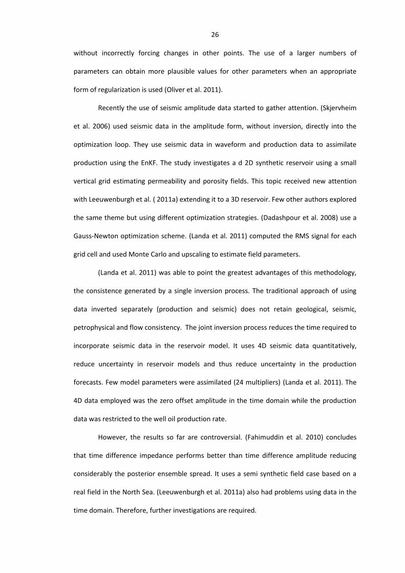
Recently the use of seismic amplitude data started to gather attention. (Skjervheim
et al. 2006) used seismic data in the amplitude form, without inversion, directly into the
optimization loop. They use seismic data in waveform and production data to assimilate
production using the EnKF. The study investigates a d 2D synthetic reservoir using a small
vertical grid estimating permeability and porosity fields. This topic received new attention
with Leeuwenburgh et al. ( 2011a) extending it to a 3D reservoir. Few other authors explored
the same theme but using different optimization strategies. (Dadashpour et al. 2008) use a
Gauss-Newton optimization scheme. (Landa et al. 2011) computed the RMS signal for each
grid cell and used Monte Carlo and upscaling to estimate field parameters.
(Landa et al. 2011) was able to point the greatest advantages of this methodology,
the consistence generated by a single inversion process. The traditional approach of using
data inverted separately (production and seismic) does not retain geological, seismic,
petrophysical and flow consistency. The joint inversion process reduces the time required to
incorporate seismic data in the reservoir model. It uses 4D seismic data quantitatively,
reduce uncertainty in reservoir models and thus reduce uncertainty in the production
forecasts. Few model parameters were assimilated (24 multipliers) (Landa et al. 2011). The
4D data employed was the zero offset amplitude in the time domain while the production
data was restricted to the well oil production rate.
However, the results so far are controversial. (Fahimuddin et al. 2010) concludes
that time difference impedance performs better than time difference amplitude reducing
considerably the posterior ensemble spread. It uses a semi synthetic field case based on a
real field in the North Sea. (Leeuwenburgh et al. 2011a) also had problems using data in the
time domain. Therefore, further investigations are required.

27
Another possibility to incorporate time-lapse data into the history matching
workflow is the use of crosswell data. (Abubakar et al. 2013) used inverted seismic crosswell
and production data to estimate permeability in a synthetic model using iterative Gauss-
Newton optimization. This study was based on (Liang et al. 2011). They used the same
methodology and model to incorporate electromagnetic and production data.
At higher acquisition frequencies the velocity dispersion phenomena delivers
valuable information about the fluid displacement in the media (Biot 1956). This can be
modeled using Biot velocity model and be used as a petrophysical model in an analogous
way of traditional Gassmann’s fluid displacement equation. Velocity can be mapped using a
crosswell tomography. It leads to a smaller area coverage but the advantages of this method
rely on the lower cost and higher reproducibility of the same especially in onshore fields
were time-lapse data is still a major challenge.
1.4 Outline of this thesis
In the Chapter 2 the basic concepts of history matching are introduced. The brief
idea behind history matching is discussed. The evolution of the methods used to perform
history matching is detailed among them manual, gradient based (assisted) and EnKF.
Disadvantages and advantages of the methods are highlighted as well as the workflow
required to perform history matching.
In the Chapter 3 the use of seismic data and time lapse data is discussed. A general
overview of seismic acquisition and its applications is presented. Their use for time lapse
acquisitions is described and its implications for reservoir management are discussed. The
link between petrophysics and reservoir properties is discussed. Gassmann’s equations for
fluid displacement and Biot velocity model are introduced. Their applicability and limitations
are pointed and improvements discussed.

28
In chapter 4 the reservoir simulation model used to perform the simulations
presented in this thesis were presented. The measurement errors are estimated and the
initial ensemble is forwarded in time and discussed. After it the results using only production
data were introduced and discussed. The use of seismic impedance data and production
data was demonstrated as a better alternative to production data alone. Finally the use of
velocity maps using Biot velocity model to link reservoir and subsurface information was
demonstrated and evaluated against other methods. The use of crosswell tomography was
proposed and evaluated.

29
Chapter 2 History Matching
2.1 Basic Concepts of History Matching
The purpose of history matching is to update uncertain model parameters, such as
permeability, porosity, critical water saturation, fault multipliers, aquifer strength, and many
others to better match the observed quantities such as gas oil rate (GOR), oil production
rate (OPR), water cut (WCT), as well as any other available data. History matching is an
important step to obtain more accurate models to describe the reservoir thus improving the
capability of producing accurate forecasts. It is important to realize that history matching
does not mean only predicting reservoir behavior. The main goal of history matching is to
improve the reservoir characterization and consequently reduce the risk exposure of the
investment. Uncertainty characterization has gained great importance in oil investments
which is often the case in the oil industry. It imposes the generation of multiple history
matched models to evaluate production uncertainty.
History matching is an under-determined inverse problem in which instead of using
reservoir model variables to predict reservoir performance (forward simulator) it uses
observed reservoir behavior (production data, seismic data and etc.) to estimate reservoir
variables that have caused this behavior (Oliver et al. 2011).
The history matching process is one of the most complex parts of a reservoir
simulation study. It used to be a manual procedure of trial and error that requires a lot of
experience and knowledge of the field. The solution is non-unique and can lead to several
scenarios. It is caused by the fact that several parameters combinations can lead to the same

30
final result but these combination of parameters may not have proper geophysical
significance for the reservoir (Portella et al. 2005). Reservoir modeling not only needs to
reproduce historical data, it must also be consistent with all available static data (core logs,
well logs, seismic data) and dynamic data (well production data, tracer concentration, 4D
seismic data). It must integrate the most updated information about the reservoir and the
associated uncertainty to allow for real time decisions (Seiler et al. 2009).
Errors present in the data can degrade the results. In general, there are important
uncertainties when dealing with large-scale models like a reservoir simulator due to the
small amount of available data and its sparse distribution. The use of 4D seismic images
allows the estimation of pressure and saturation changes during the lifetime of the
reservoir. Until recently, it was quite difficult to incorporate 4D seismic data in reservoir
modeling due to the lack of specialized software that could deal with this large data set.
Time-lapse 4D surveys were used in qualitative or semi-quantitative ways, mostly to identity
unexplored compartments in the reservoir.
In conventional history matching (manual and adjoint based methods) a cross
function is usually defined measuring the misfit between the model output and the data the
problem then reduces to the optimization of this function with respect to the unknown
reservoir parameters. The most challenging problem is related to the nature of the cost
function, which is non-convex. This means that the objective function to be minimized has
several local minima. Thus, the likelihood of the optimization converging to a local minima
instead of the global minima is high. The most common methods make use of gradient
optimization methods to minimize the cost function. Traditional history matching methods
often include a low number of model parameters in the optimization process typically
identified from a sensitivity study to improve convergence rate of the optimization.
Schlumberger developed a software package to assists with history matching
namely Simulation Optimization (SimOpt) (Gosselin et al. 2003). This software was the first

31
one to introduce time lapsed seismic data to reservoir modeling. The software is a joint
project sponsored by the European Commission, Total E&P, Norsk Hydro (Statoil) and
Schlumberger to develop an industrial application to incorporate of 4D seismic data to
improve reservoir modeling.
The main challenge in this project was the construction of a petro-elastic model. It
was done using ad-hoc solutions from the partners and it is not scalable. Each one of the
partners wrote its own petro-elastic model to fulfill its own needs. The PEM cannot be
extended to a general case, which will make it inappropriate to other reservoir models.
Other major discoveries were made during this project. Poisson’s ratio inversion was noisy,
acoustic impedances led to improved results. There is a major drawback with the use of this
software because its computational cost increase exponentially with the amount of
parameters been assimilated. Non gradient optimization methods are still under
development (Gosselin et al. 2003).
Ensemble methods have gained attention recently due to their capacity to generate
multiple history-matched models. EnKF can provide a measure of the uncertainty in
reservoir performance predictions making it a powerful tool for reservoir engineers,
geologists and decision makers. The computational cost of EnKF based methods does not
depend on the number of parameters being estimated. Therefore, a larger number of
parameters can be estimated. This will allow the data to have its values modified in some
areas while retaining plausible values for the other variables. Moreover EnKF was shown to
perform reasonably well and give better results than a model based on a manual history
matching (Bianco et al. 2007). Among the advantages of using the EnKF are the fact that it
does not require the implementation of adjoint for computing gradients, which makes it
independent of the simulator, allowing it to be used with commercial implementations. In
EnKF the data is assimilated sequentially making it well suited for closed loop reservoir
management problems (Emerick 2012).

32
The History Matching process can include more parameters than porosity and
permeability. It can also include initial oil water contact, gas oil contacts, net to gross ratio,
fault multipliers and many others. One of the great advantages of EnKF based methods over
other approaches is its ability to estimate both the model state and parameters and it can be
easily extended to include other variables and data types.
2.2 Manual Assisted History Matching
In a manual history matching study, the first step is to ensure that a good pressure
match in the reservoir is found. The study starts with a material balance evaluation. It
evaluates the water influx from the aquifer, fluid expansion effects, compressibility effects
and water injection. The usual unknown parameters are the aquifer strength and water
saturation and oil water contact. A match is obtained by adjusting the aquifer pore volume,
aquifer transmissibility and strength, permeability multipliers, rock compressibility and the
vertical to horizontal ratio of the permeability. Then the oil production rate and water cut
are matched.
Traditional methods for assisted history matching are constrained do include a low
number of model parameters in the optimization process. The history matching process is
then performed using only the most influential parameters identified by a sensitivity study.
The other ones can be set to be static (a fixed value) because it will not change the result
significantly. A significant uncertainty in some parameters can lead to complementary
actions like reprocessing the seismic data. Such decisions are made with the help of a Pareto
plot.
The sensibility study is conceived by setting a base value (static value) for each of the
parameters and estimating its variance. For each of the parameters the model is evaluated
for its extreme values. The other values are frozen at their base value. A fair comparison of
the impact of each parameter must take in consideration the shape of the distribution. It is
33
important that a low value represents the P10 value, the base value the P50 value and the
maximum value the P90 value of that parameter (Doren et al. 2012).
Best practices suggest a layer by layer approach to facilitate the history matching
approach (Williams et al. 1998). First, the reservoir is treated as a single layer model to
adjust the aquifer parameters (material balance). Then layer-by-layer is adjusted starting by
the bottom to the top as the water displacement takes place.
Manual history matching usually involves several subjective choices, which are not
properly documented. The use of computed assisted techniques favors a more reproducible
approach (Peters et al. 2011). An experienced professional dealing with a complex field may
take up to one year of work to match 25 years of production data (Oliver et al. 2011).
The first output of the history matching process is usually consistent with production
data buy it is not consistent with the rest of the data, therefore this is not mature. There are
still unfeasible parameter values apparently tend to compensate the model features that
were not included in the study. These unrealistic numbers give information about flaws in
the model that needs to be corrected. Development possibilities are further investigated by
performing a no further activity (NFA) forecast and looking to the oil saturation and reservoir
pressure distribution at the end of the NFA forecast.
2.3 Gradient Based Assisted History Matching
The gradients of the mismatch objective function with respect to the parameters are
either analytically or numerically calculated Eq. 2.3. If the number of parameters that needs
to be estimated is large, the use of analytical gradients turns to be computationally
advantageous. The most used ones are the adjoint-based methods and the streamline
based methods. The main disadvantage of the adjoint method is the cost to implement the
system of linearized equations and their iterative solution into the reservoir simulator.

34
Gradient based methods could yield better results than EnKF with weakly non-linear models,
but at a greater computational cost and implementation efforts (Hanea et al. 2010).
The framework used to history match a reservoir using gradient-based methods is
not probabilistic, but several initial models can be created and mismatched in parallel to
produce several output models, allowing the reservoir engineer to choose the best scenario
this is however computationally demanding.
Consider a discrete non-linear dynamic system given by Eq. 2.1 where
denotes a state vector of model variables at time , is the non-
linear dynamical operator that integrates the model state form to . is the
model error (system noise) accounting for model uncertainties. While the observations of
the state variables are available through the observational system Eq. 2.2.
( ) Eq. 2.1
( ) Eq. 2.2
( )
(
) (
)
∑( ( ))
( ( ))
Eq. 2.3
is a vector of observations at time ,
is the
observation operator. The observation errors are represented by instrumental and
systematic errors with Gaussian distribution with zero mean and covariance . Model and
observation errors are assumed to be independent. The objective function is given by Eq.
2.3.

35
2.4 EnKF History Matching
Ensemble methods are gaining interest as a powerful tool for history matching. The
Kalman filter is an efficient recursive estimator of the state of a linear dynamical system. It is
a sequential data assimilation method in which an ensemble of realizations is employed to
construct Monte Carlo approximations of the mean and the covariance of the state vector
(Emerick et al. 2012). The data is processed sequentially in time (new data are easily
accounted for when they arrive). The method allows the estimation of a large number of
poorly known parameters such as facies characterization, porosity, permeability and etc..
One useful feature of the EnKF is that the forecasts of reservoir performance can be
made by running the simulator forward in time from the most recent data assimilation time
(analysis step). The mean of the entire ensemble forecast provides an estimate of the true
forecast. It is also possible to obtain the uncertainty in the estimated forecast (Seiler et al.
2009).
These predictions with uncertainty estimates provide the reservoir management
team with valuable information. Different production schemes and drainage strategies can
be evaluated as well as the associated risk (Seiler et al. 2009). One way of representing the
geological uncertainty embedded in the reservoir model is to work with an ensemble of
model realizations. In ensemble methods uncertainties are treated statically by adding a
random perturbation to the baseline value and exploiting the statistical relationships
between these parameters and simulated production variables (Leeuwenburgh et al. 2011b).
The EnKF method is not limited by the number of parameters. The dimension of the
inverse problem is reduced to the number of realizations included in the ensemble (Seiler et
al. 2009). The large number of observations that can be assimilated by EnKF is extremely
useful due to the increasing use of intelligent field technologies (intelligent wells, and so on).
Without decent predictions the full potential of the intelligent technologies cannot be

36
exploited (Peters et al. 2011). Even using EnKF to accurately represent all the possible
variations of a large number of geological features has limitations. A large number of
ensembles is required for this task, which comes with a greater computational cost.
Once the initial uncertainties have already been identified and quantified, they are
used to create ensembles representing the possible geological models describing the
reservoir. The seismic data is sparse in time while production data is sparse in space. Few
seismic surveys are available along the lifetime of the reservoir while the production data is
only available at the well locations.
Depending on the modeling objectives the history matching procedure can be
performed at reservoir level or at well by well level if the desired objective is to find new
locations for infill wells (Doren et al. 2012). Many geological features are local in nature
therefore they are overlooked by global scalar multipliers. One way to overcome this
limitation is by using ensembles, employees an array of local multipliers instead of a single
scalar.
The EnKF uses a sample or ensemble of state vectors, Eq. 2.4 where denotes the
number of ensemble members. At every forecast step, all ensemble members are integrated
forward in time with the dynamical model in Eq. 2.1. The state estimate and the associated
covariance matrix are estimated respectively as Eq. 2.5 and Eq. 2.6.
{ } Eq. 2.4
∑
Eq. 2.5
37
∑(
)(
)
Eq. 2.6
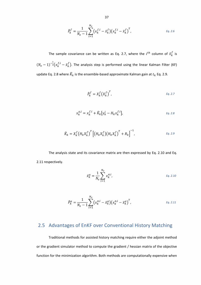
The sample covariance can be written as Eq. 2.7, where the column of
is
( )
(
). The analysis step is performed using the linear Kalman Filter (KF)
update Eq. 2.8 where is the ensemble-based approximate Kalman gain at Eq. 2.9.
(
) Eq. 2.7
[
] Eq. 2.8
(
) [(
)(
) ]
Eq. 2.9
The analysis state and its covariance matrix are then expressed by Eq. 2.10 and Eq.
2.11 respectively.
∑
Eq. 2.10
∑(
)(
)
Eq. 2.11
2.5 Advantages of EnKF over Conventional History Matching
Traditional methods for assisted history matching require either the adjoint method
or the gradient simulator method to compute the gradient / hessian matrix of the objective
function for the minimization algorithm. Both methods are computationally expensive when

38
the number of parameters been estimated or the number of observed data are big. One of
the biggest advantages of the EnKF formulation is that it does not require the solution to the
adjoint matrix therefore it is independent of the simulator (Dong et al. 2006).
In practice, this makes the ensemble Kalman filter more capable of handling large
parameter spaces because the Kalman gain matrix does not depend of the size of the
ensemble. This advantage is imperative for complex reservoirs where several parameters
need to be estimated.
In conventional history matching a sensitivity study is performed to investigate the
most critical parameters affecting history matching and by doing it reducing the number of
parameters assimilated. For an EnKF study the sensitivity study is required to quantify the
uncertainty of the model and include it in the ensembles.
Unfortunately, the EnKF still have some limitations due to the Gaussianity
assumption used for the update step as well as the limited size of the ensembles. The
reduction in the ensemble variance during the assimilation step might be excessive and
incorrect. The small number of ensembles limits number of degrees of freedom to history
matched data. Nonphysical values updates in model parameters and state variables are not
prohibited by the EnKF methodology (Emerick 2012).
2.6 History Matching Workflow
A history matching workflow can be divided in 3 major steps:
1. Identification of the prior information and its uncertainty.
2. Identification of the information to be used and its uncertainty.
3. Solution of the history matching problem.
The first step is the most difficult and time consuming (Peters et al. 2011). At the
begging of the workflow, it is assumed that the static model, the basic data and the

39
production data have been quality checked. The model objectives have been identified. A
starting reservoir model non-history matched is available at the appropriate scale (the data
types have different resolution in time and space). During the first step a base model will be
produced. It is important to obtain a reliable base model (reasonably close to the truth).
Major conceptual errors cannot be fixed by matching model parameters, updates will
become unrealistic once the updates will try to compensate for all model errors. The
uncertainty of parameters being used will also be quantified during the first step. The major
difference of a conventional sensitivity test and a test intended to take advantage of EnKF is
the fact that EnKF can deal with a larger number of parameters being assimilated. Therefore,
an EnKF workflow aims to quantify the uncertainties in the grid parameters and not of the
modeling concepts (Peters et al. 2011).
A procedure is required to produce the initial ensemble. The most uncertain
parameters are perturbed by its uncertainty to generate a set of models. The ensemble (set
of models) must be consistent with the full uncertainty. For statistical reasons it is important
to choose it large enough to be able to fully represent all the range of geological models
describing the reservoir. This procedure concludes the first step in the history matching
process.
In the second step the production data are analyzed with respect to the data used to
constrain the model (oil rates) and also to the other observations that were not used in the
history matching workflow. The constrains are also perturbed to take into account their
uncertainty regardless whether they were estimated or not. During this step the initial
ensemble is screened to make sure if it has enough coverage to describe the uncertainties in
the observations. This indicates the quality of the quantified uncertainty. The first step to
screening the ensemble is to run it forward it in time and comparing with actual
observations. Multidimensional scaling (MDS) tools are used to visualize the ensemble in
one plot (Peters et al. 2011).

40
Finally, the history matching will be performed in the last step. After the history
match the estimate must be checked to ensure that the updates are within the limits of the
uncertainty of the parameters and if the data fit is acceptable. Extreme updates (outside of
the specified uncertainties) indicate improper specification of the model and / or its
uncertainties.

41
Chapter 3 Time-Lapse Seismic Data
3.1 Seismic data
Drilling is an expensive and extremely risky activity. Current projects can exceed
hundreds of millions of dollars to drill in deep water offshore fields. The decision to seek
such investment is more than ever heavily based on the interpretation of seismic data and
other relevant data.
A seismic survey images the subsurface by gathering elastic wave information from
it. Seismic waves are generated at the surface and propagated through the medium being
reflected along interfaces between the layers of different impedance. The returning waves
are recorded, they contain information about the properties of the medium along their path.
The seismic signal combines source wavelet and medium response. None of them is
accurately known. Using a proper input wavelet during the inversion process is important to
deconvolve the data and obtain the medium response mostly in the form of reflectivity
series.
Until few decades ago, seismic data was acquired along 2D lines. Now the
acquisition of 3D data became economically attractive. It is common for surveys nowadays
to use multicomponent seismic (recording P and S waves). The P wave carries information
about changes in pressure and saturation while S waves are only sensitive to pressure
changes. S waves are insensitive to the fluid present in the medium because fluids cannot
sustain shear stress. Therefore, in a porous medium the S wave travels through the rock
matrix while P waves travel through rock and fluid. The bulk modulus will be affected by the

42
changes in saturation because P waves travel through the rock matrix and fluid while shear
modulus remain constant once S waves do not travel through the fluid (Han et al. 2004).
To predict lithology, fluid and porosity properties seismic data must be used to
obtain density, P and S-wave velocity of the layers. This procedure is called elastic inversion.
Porosity can be obtained directly from the seismic data (Rasmussen et al. 1996).
Permeability usually cannot, the inversion is less sensitive to permeability, and correlations
between seismic attributes and porosity must be obtained from core and well logs.
Information about the medium density, bulk moduli and pore bulk moduli can only be
decoupled knowing the P and S velocities. The multicomponent seismic acquisition is then
used since acoustic and elastic properties are needed to estimate these rock properties.
Offshore multicomponent seismic requires the use of ocean bottom cable (OBC) because S
waves do not travel through water. This make the acquisition process even more expensive
(Dijkstra et al. 2003).
Another way to obtain elastic information of the subsurface is by the use of
Amplitude Versus Offset (AVO) inversion. The reflection at the interface between P and S
waves is angle dependent. The amplitudes of reflected and transmitted P- and S-waves for
any angle of incidence are given by Zoeppritz equation (Aid et al. 1980). By using different
offsets (incidence angles) indirect information is obtained about the S waves. Thus, a
conventional seismic survey can be used to provide information about saturation and elastic
parameters in the medium.
Recently seismic surveys of a same area obtained at times became available. This is
known as time-lapse seismic data and contains relevant information for reservoir
management.

43
3.2 Time-lapse Seismic Data
A single snapshot of the reservoir (taken by performing a 3D seismic acquisition)
cannot be used to uniquely separate geological and fluid flow components of the reservoir
model. Time-lapse seismic data also known as 4D seismic data consist of a set of seismic
surveys obtained at different times. By investigating time-lapse seismic images it is possible
to remove the time invariant component (geological model) retaining an image of the
dynamic model behavior which includes changes in fluid saturation, pore pressure, and
temperature. Well logs and other types of laboratorial data are required to calibrate the
model providing a unique solution for variations in pressure and saturation (Lumley et al.
1998).
The traditional use of time-lapse seismic data consists of using inverted images of
seismic attributes obtained at different times subtracted from each other. The time-lapse
signal is the difference between the two surveys and shows changes in dynamic properties
of the subsurface. The time-lapse signal changes as the reservoir conditions change from an
oil-saturated reservoir to water saturated one. The rock compressibility increases due to gas
migration. It gives rise to a seismic signal-softening (the impedance decreases), while the
rock compressibility decreases due to water injection hardening the signal. The 4D seismic
data has high lateral resolution but low vertical resolution when compared to well logs
(Lumley et al. 1998).
Certain conditions must be satisfied before a 4D seismic study can be considered,
reproducibility must be satisfied, and the predicted signal difference between surveys due to
production effects must be higher than the uncertainty in the dataset. High porosity rocks
like unconsolidated sandstone or heavily fractured rock are ideal for 4d seismic monitoring
while highly consolidated or cemented sandstones or rigid carbonates are poor candidates
for 4D seismic monitoring. The reason for this is that reservoir rocks with low compressibility

44
do not show a strong pore fluid saturation response and tend to be unfavorable to 4D
seismic (Lumley et al. 1998).
Once the required conditions (significant signal) are ensured, the major source of
risk in a time-lapse study is related to the repeatability of the acquisition. Acquisition
artifacts have to be eliminated by reproducing the setup and reprocessing of the data sets.
Cross equalization is required to cross calibrate the datasets (Dijkstra et al. 2003).
Repeatability is difficult to be obtained because the environment changes over time (due to
the inclusion of production facilities and etc.). Another challenge is the use of older datasets
collected with outdated technologies. When they were collected their future use in 4D
studies was not anticipated thus reproducibility issues must be considered.
Summarizing the time-lapse data is a valuable resource to constrain dynamic
behavior of the reservoir and improve production forecasting when these conditions are
met.
3.3 Crosswell Seismic Data
A crosswell seismic experiment consist in the acquisition of seismic data at reservoir
depth by inserting an array of sources in one well and an array of receivers in another well.
The signal travels between the wells and contain information about the traversed path.
Crosswell seismic experiments provide high-resolution spatial data due to the higher
frequencies used for the subsurface imaging. The crosswell imaging is a transmission
technique where sources and receivers are located opposite to each other. Therefore,
attenuation of the signal is much smaller than surface seismic surveys using reflected waves
from the subsurface. Crosswell surveys are sensitive to small velocity variations over thin
zones. This is ideal to monitor changes in early development stages of field production (Liang
et al. 2011).

45
The use of crosswell tomography has found extensive use in EOR recovery
applications by steam injection to track the flooding process due to temperature variations
(Droujinina et al. 2001; Maamari et al. 2011; Rocco et al. 2011). Due to temperature
increases (steam injection), the acoustic velocity decreases. Few quantitative uses for this
type of data were attempted so far (Liang et al. 2011; Abubakar et al. 2013).
Crosswell seismic data provides P and S wave first arrivals that can be used to
compute velocity tomograms. The velocity changes can be mapped over time and linked to
fluid displacement in the reservoir.
3.4 Reservoir Management and Seismic Data
Good reservoir management practices aim to maximize investment return (profit)
given geological, environmental, technical and political constraints. This is usually obtained
by improved forecasting capabilities leading to better understanding of the project and
consequently lower risk associated with future investments. This is a multidisciplinary task
where intensive collaboration between geologists, petrophysicists, reservoir engineers and
geophysicists is required.
Time-lapse data is a powerful tool to mitigate drilling risk for infilling projects, to
find unswept oil, which represents the major source of revenue to oil companies, it and can
extend oil field lifetime and profitability. It also can be used to monitor fluid contacts.
Monitoring fluid contacts is economically extremely important. If oil migrates out of the oil
zone it will significantly reduce the amount of oil that can be recovered due to capillary
pressure constrains. It is also important for tracking the injected fluids because they control
the efficiency of the flooding process .They also account for a major cost component in the
project especially if Enhanced Oil Recovery (EOR) is being used because the fluids in this case
are expensive. Preventing premature water breakthrough and therefore increasing the
sweep efficiency is also possible using 4D studies (Lumley et al. 1998).

46
Consequently reservoir management is a complex task that relies on simulation
models to forecast future behaviors.
3.5 Different Types of Data Employed
For reservoir purposes, seismic data is routinely inverted for elastic properties. The
inversion of seismic data to acoustic or elastic impedance is complex, sometimes multiple
inversions are required to provide relevant data for reservoir engineering purposes.
There are several ways to incorporate seismic data in a reservoir framework. The
most used form so far is the petro-elastic inversion. The 4D seismic data can be used in
several basic forms some of these are fluid saturation, pressure, seismic impedance, seismic
amplitude, bulk modulus, Poisson’s ratio and acoustic velocity. The selection of the type of
data being used defines the meeting point between geophysics and reservoir engineering.
For reservoir engineers the easiest form to understand and analyze 4D seismic data
is to invert it to obtain pressure and saturation. This is due the fact that the reservoir
simulator calculates pressure and saturation by default to be able to estimate production
data. However this is the most complex form of processing 4D seismic data because it
requires two inversions procedures (Landa et al. 2011).
The simplest form of seismic processing occurs at the level of seismic traces because
there is no need for seismic inversions. However this is the most difficult setup for the
reservoir engineer because it is difficult to associate seismic traces with reservoir properties
(Landa et al. 2011).
Most often petro-elastic properties (acoustic and elastic impedance) are used. They
are calculated from the simulation model (using grid properties like density, saturation and
etc.). It does not require the generation of seismic data (forward modeling). The major
disadvantage of this procedure is handling uncertainty. The difference between real and
synthetic data is required during the assimilation process. The seismic data needs to be

47
inverted for elastic properties before compared with simulated properties. Inverting seismic
data (real data) is not trivial, inversion is an art by itself and uniqueness cannot be
guaranteed (Sagitov et al. 2012). On the other hand, producing synthetic acoustic impedance
is fairly easy by just applying a rock physics package to the reservoir model.
Another possibility is by the direct incorporation of seismic information in the time
domain. Forward modeling is used to generate seismic data, it is usually performed by a
convolution. The amount of time required to perform this task is reasonably low when
compared with the amount of time to run the forward simulations. It does not require the
data to be inverted, however the amount of data present in the mismatch function increases
considerably, the data requires processing for noise removal and normalization. Seismic
forward modeling is associated with errors due to the fact that it does not take in
consideration many factors during the simulation, this affect the misfit response
(Fahimuddin et al. 2010).
Few researches have used seismic data without inversion directly to improve the
flow information. Among them (Skjervheim et al. 2006; Dadashpour et al. 2008; Dadashpour
et al. 2009; Fahimuddin et al. 2010; Landa et al. 2011; Leeuwenburgh et al. 2011a).
(Dadashpour et al. 2008; Dadashpour et al. 2009) use a Gauss-Newton optimization
scheme while (Skjervheim et al. 2006; Fahimuddin et al. 2010; Leeuwenburgh et al. 2011a)
used EnKF. In these works seismic data was generated by a convolution approach,
convolving a wavelet signature with an array of reflectivity coefficients. This method only
takes into consideration P waves and does not account for attenuation, therefore it can be
used only for a small time window. The seismic signal is then taken only at reservoir depth,
therefore making this assumption possible (Leeuwenburgh et al. 2011a). A worst match was
obtained using amplitude seismic data when compared with seismic impedance results. This
may be explained by the larger uncertainty observed in the data and the lower correlation
between this data and porosity and permeability (Fahimuddin et al. 2010).

48
The traditional approach of using data inverted separately (production and seismic)
does not retain geological, seismic, petrophysical and flow consistency. The joint inversion
process reduces the time required to incorporate seismic data in the reservoir model. It uses
4D seismic data quantitatively, reducing uncertainty in reservoir models and thus reducing
uncertainty in the production forecasts (Landa et al. 2011).
3.6 Petro-Elastic Model
Rock physics is an essential link connecting seismic data to the presence of in situ
hydrocarbons and to reservoir characterization. This link is obtained through the petro-
elastic model (PEM). The PEM is defined based on well log analysis, rock physics and
available laboratory data. This is the link between the reservoir engineering and geophysics.
The link is a set of equations used to calculate three elastic parameters, Poisson’s ratio, P
and S impedance from simulated pressure, saturation porosity and fluid content.
The equations normally used are the Batzle and Wang equations for the fluid
properties and the Gassmann’s equations for rock properties (Reiso et al. 2005). These
relations predict elastic properties of saturated porous medium from simulated fluid and
static rock properties making a bridge between fluid flow and wave propagation domains.
The most widely used and successful method for determining the effects of production
induced fluid change is the Gassmann substitution method (Gassmann 1951) shown in the
Eq. 3.1. It predicts the increase in the effective bulk modulus Ksat and shear modulus of the
saturated rock Gsat based on the porosity and bulk modulus of the dry rock , fluid
, rock matrix and shear modulus of the dry rock .
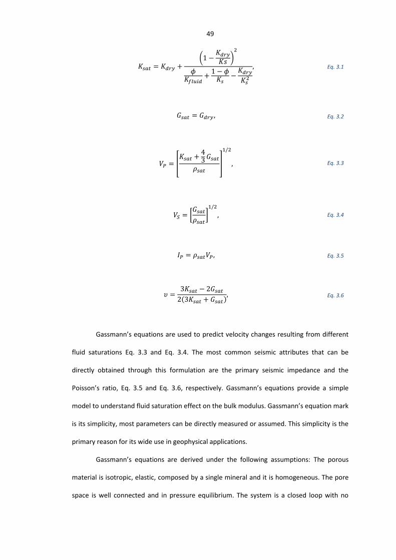
49
(
)
Eq. 3.1
Eq. 3.2
[
]
Eq. 3.3
[
]
Eq. 3.4
Eq. 3.5
( )
Eq. 3.6
Gassmann’s equations are used to predict velocity changes resulting from different
fluid saturations Eq. 3.3 and Eq. 3.4. The most common seismic attributes that can be
directly obtained through this formulation are the primary seismic impedance and the
Poisson’s ratio, Eq. 3.5 and Eq. 3.6, respectively. Gassmann’s equations provide a simple
model to understand fluid saturation effect on the bulk modulus. Gassmann’s equation mark
is its simplicity, most parameters can be directly measured or assumed. This simplicity is the
primary reason for its wide use in geophysical applications.
Gassmann’s equations are derived under the following assumptions: The porous
material is isotropic, elastic, composed by a single mineral and it is homogeneous. The pore
space is well connected and in pressure equilibrium. The system is a closed loop with no
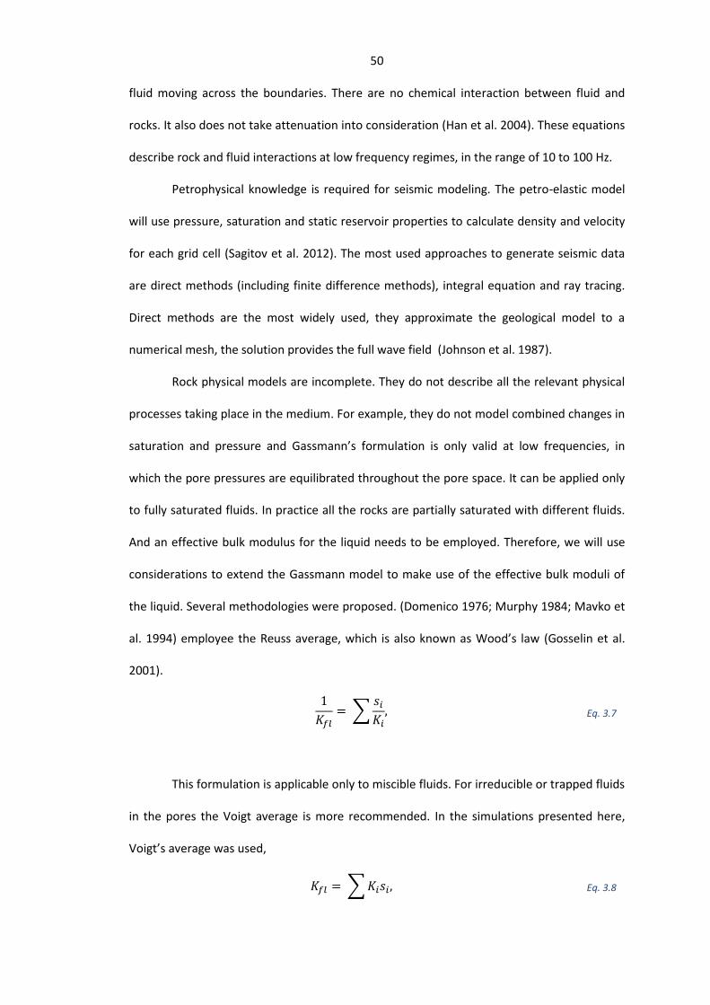
50
fluid moving across the boundaries. There are no chemical interaction between fluid and
rocks. It also does not take attenuation into consideration (Han et al. 2004). These equations
describe rock and fluid interactions at low frequency regimes, in the range of 10 to 100 Hz.
Petrophysical knowledge is required for seismic modeling. The petro-elastic model
will use pressure, saturation and static reservoir properties to calculate density and velocity
for each grid cell (Sagitov et al. 2012). The most used approaches to generate seismic data
are direct methods (including finite difference methods), integral equation and ray tracing.
Direct methods are the most widely used, they approximate the geological model to a
numerical mesh, the solution provides the full wave field (Johnson et al. 1987).
Rock physical models are incomplete. They do not describe all the relevant physical
processes taking place in the medium. For example, they do not model combined changes in
saturation and pressure and Gassmann’s formulation is only valid at low frequencies, in
which the pore pressures are equilibrated throughout the pore space. It can be applied only
to fully saturated fluids. In practice all the rocks are partially saturated with different fluids.
And an effective bulk modulus for the liquid needs to be employed. Therefore, we will use
considerations to extend the Gassmann model to make use of the effective bulk moduli of
the liquid. Several methodologies were proposed. (Domenico 1976; Murphy 1984; Mavko et
al. 1994) employee the Reuss average, which is also known as Wood’s law (Gosselin et al.
2001).
∑
Eq. 3.7
This formulation is applicable only to miscible fluids. For irreducible or trapped fluids
in the pores the Voigt average is more recommended. In the simulations presented here,
Voigt’s average was used,
∑ Eq. 3.8
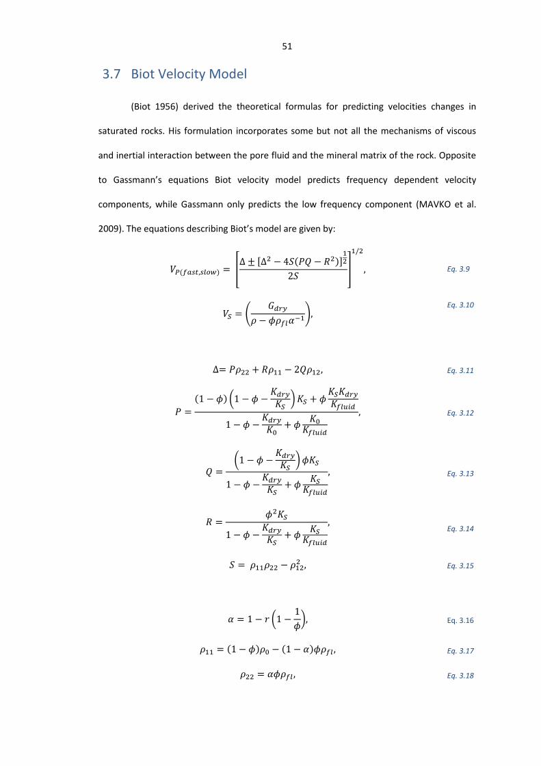
51
3.7 Biot Velocity Model
(Biot 1956) derived the theoretical formulas for predicting velocities changes in
saturated rocks. His formulation incorporates some but not all the mechanisms of viscous
and inertial interaction between the pore fluid and the mineral matrix of the rock. Opposite
to Gassmann’s equations Biot velocity model predicts frequency dependent velocity
components, while Gassmann only predicts the low frequency component (MAVKO et al.
2009). The equations describing Biot’s model are given by:
( ) [ [ ( )]
]
Eq. 3.9
(
)
Eq. 3.10
Eq. 3.11
( ) (
)
Eq. 3.12
(
)
Eq. 3.13
Eq. 3.14
Eq. 3.15
(
) Eq. 3.16
( ) ( ) Eq. 3.17
Eq. 3.18
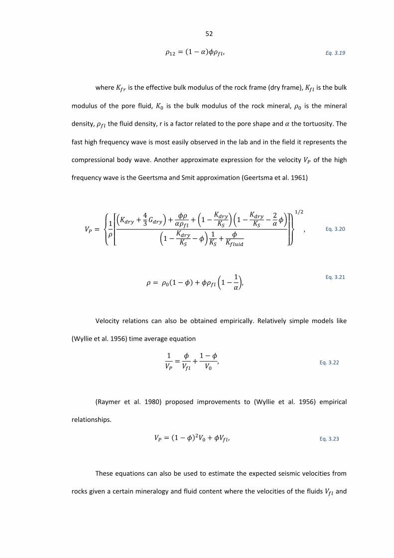
52
( ) Eq. 3.19
where is the effective bulk modulus of the rock frame (dry frame), is the bulk
modulus of the pore fluid, is the bulk modulus of the rock mineral, is the mineral
density, the fluid density, r is a factor related to the pore shape and the tortuosity. The
fast high frequency wave is most easily observed in the lab and in the field it represents the
compressional body wave. Another approximate expression for the velocity of the high
frequency wave is the Geertsma and Smit approximation (Geertsma et al. 1961)
{
[ (
)
(
) (
)
(
)
]
}
Eq. 3.20
( ) (
)
Eq. 3.21
Velocity relations can also be obtained empirically. Relatively simple models like
(Wyllie et al. 1956) time average equation
Eq. 3.22
(Raymer et al. 1980) proposed improvements to (Wyllie et al. 1956) empirical
relationships.
( ) Eq. 3.23
These equations can also be used to estimate the expected seismic velocities from
rocks given a certain mineralogy and fluid content where the velocities of the fluids and

53
the velocity of the rock matrix is known . This model however has similar limitations as the
Gassmann’s equations. It is limited to a rock composed by a single homogeneous mineral, it
is fully saturated by a single immiscible liquid. In practice however it is usually extended to
avoid some of these limitations (MAVKO et al. 2009).
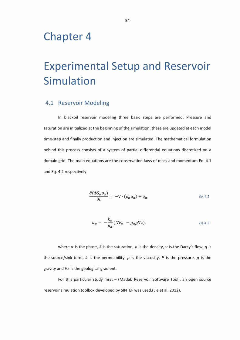
54
Chapter 4 Experimental Setup and Reservoir Simulation
4.1 Reservoir Modeling
In blackoil reservoir modeling three basic steps are performed. Pressure and
saturation are initialized at the beginning of the simulation, these are updated at each model
time-step and finally production and injection are simulated. The mathematical formulation
behind this process consists of a system of partial differential equations discretized on a
domain grid. The main equations are the conservation laws of mass and momentum Eq. 4.1
and Eq. 4.2 respectively.
( )
( ) Eq. 4.1
( ) Eq. 4.2
where is the phase, is the saturation, is the density, is the Darcy’s flow, is
the source/sink term, is the permeability, is the viscosity, is the pressure, is the
gravity and is the geological gradient.
For this particular study mrst – (Matlab Reservoir Software Tool), an open source
reservoir simulation toolbox developed by SINTEF was used.(Lie et al. 2012).

55
4.2 Synthetic Model
An identical twin experiment intended for history matching purposes was designed
to highlight the economical impact of uncertainties in the initial geological model. We
consider a two dimensional domain model consisting of one horizontal layer of 40 by 40 grid
cells of dimension 50 by 50 meters. The thickness of the layer is 25 meters. The reservoir is
composed of high quality sandstone. Petrel was used to geostatistically populate porosity
and permeability properties. The model uses water flooding as recovery strategy, the
injection is controlled by voidage replacement. A five spot pattern is used to produce the
reservoir (four producers in each one of the corners and one injector in the center). Only
two phases are considered, water and oil. The initial conditions are specified as equilibrium
conditions for the simulator. Therefore, the simulator calculates the initial pressure
distribution based on the pressure and the depth of the datum and oil contacts. The initial
saturation is assumed to be constant and equal to the connate water along the entire
domain. The simulated fluid is treated as dead oil.
The geological properties (permeability and porosity) were populated
geostatistically as seen in the Figure 2. A high permeability and porosity area is present in
the left side of the field while a lower permeability and porosity area is present in the lower
right portion of the field. The attributes are distributed following a Gaussian distribution
(Figure 3). Permeability was obtained through co-kriging using the porosity as secondary
parameter. Thus a correlation between porosity and permeability is present in the geological
model (Figure 4).
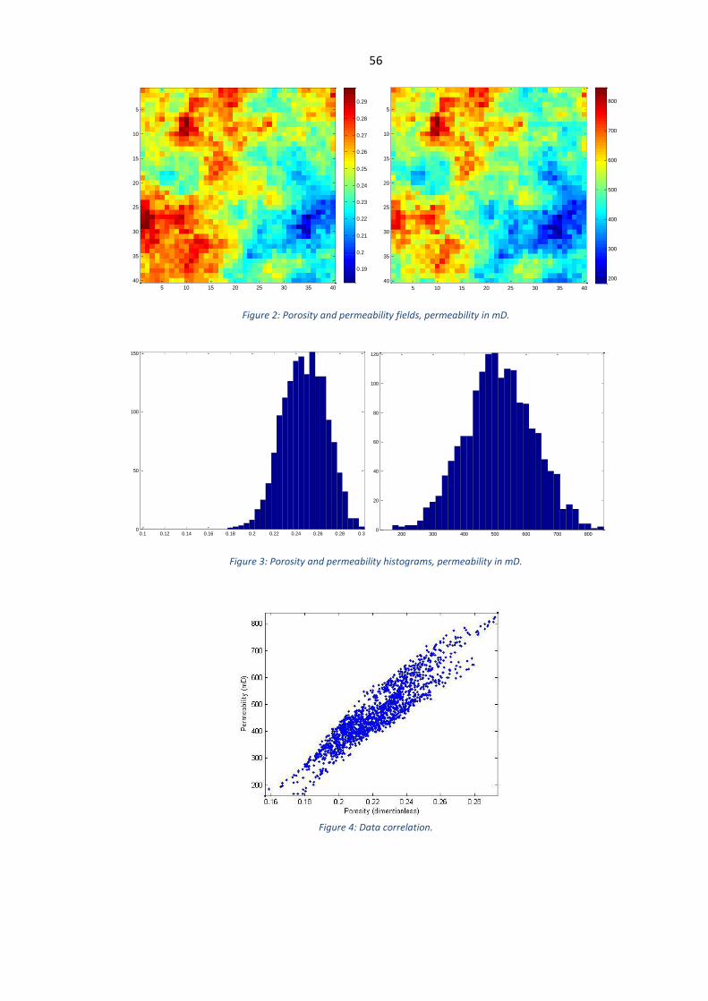
56
Figure 2: Porosity and permeability fields, permeability in mD.
Figure 3: Porosity and permeability histograms, permeability in mD.
Figure 4: Data correlation.
5 10 15 20 25 30 35 40
5
10
15
20
25
30
35
40
0.19
0.2
0.21
0.22
0.23
0.24
0.25
0.26
0.27
0.28
0.29
5 10 15 20 25 30 35 40
5
10
15
20
25
30
35
40 200
300
400
500
600
700
800
0.1 0.12 0.14 0.16 0.18 0.2 0.22 0.24 0.26 0.28 0.30
50
100
150
200 300 400 500 600 700 8000
20
40
60
80
100
120
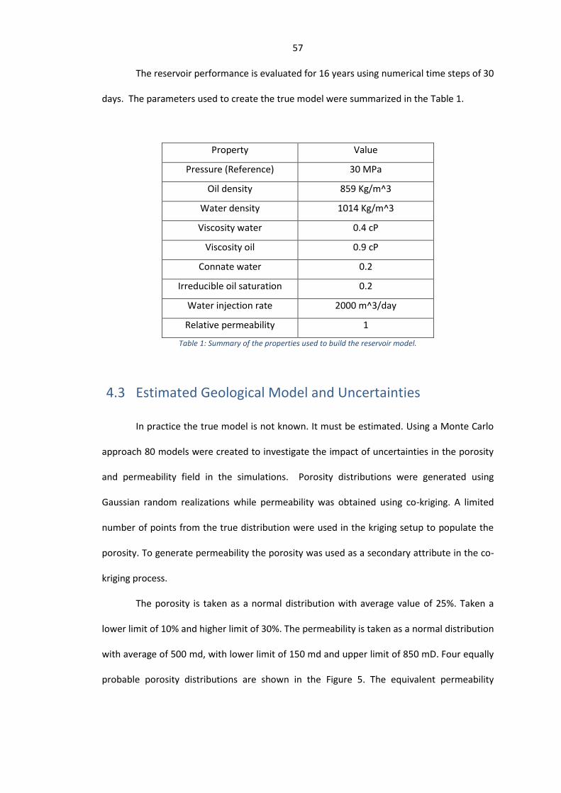
57
The reservoir performance is evaluated for 16 years using numerical time steps of 30
days. The parameters used to create the true model were summarized in the Table 1.
Property Value
Pressure (Reference) 30 MPa
Oil density 859 Kg/m^3
Water density 1014 Kg/m^3
Viscosity water 0.4 cP
Viscosity oil 0.9 cP
Connate water 0.2
Irreducible oil saturation 0.2
Water injection rate 2000 m^3/day
Relative permeability 1
Table 1: Summary of the properties used to build the reservoir model.
4.3 Estimated Geological Model and Uncertainties
In practice the true model is not known. It must be estimated. Using a Monte Carlo
approach 80 models were created to investigate the impact of uncertainties in the porosity
and permeability field in the simulations. Porosity distributions were generated using
Gaussian random realizations while permeability was obtained using co-kriging. A limited
number of points from the true distribution were used in the kriging setup to populate the
porosity. To generate permeability the porosity was used as a secondary attribute in the co-
kriging process.
The porosity is taken as a normal distribution with average value of 25%. Taken a
lower limit of 10% and higher limit of 30%. The permeability is taken as a normal distribution
with average of 500 md, with lower limit of 150 md and upper limit of 850 mD. Four equally
probable porosity distributions are shown in the Figure 5. The equivalent permeability
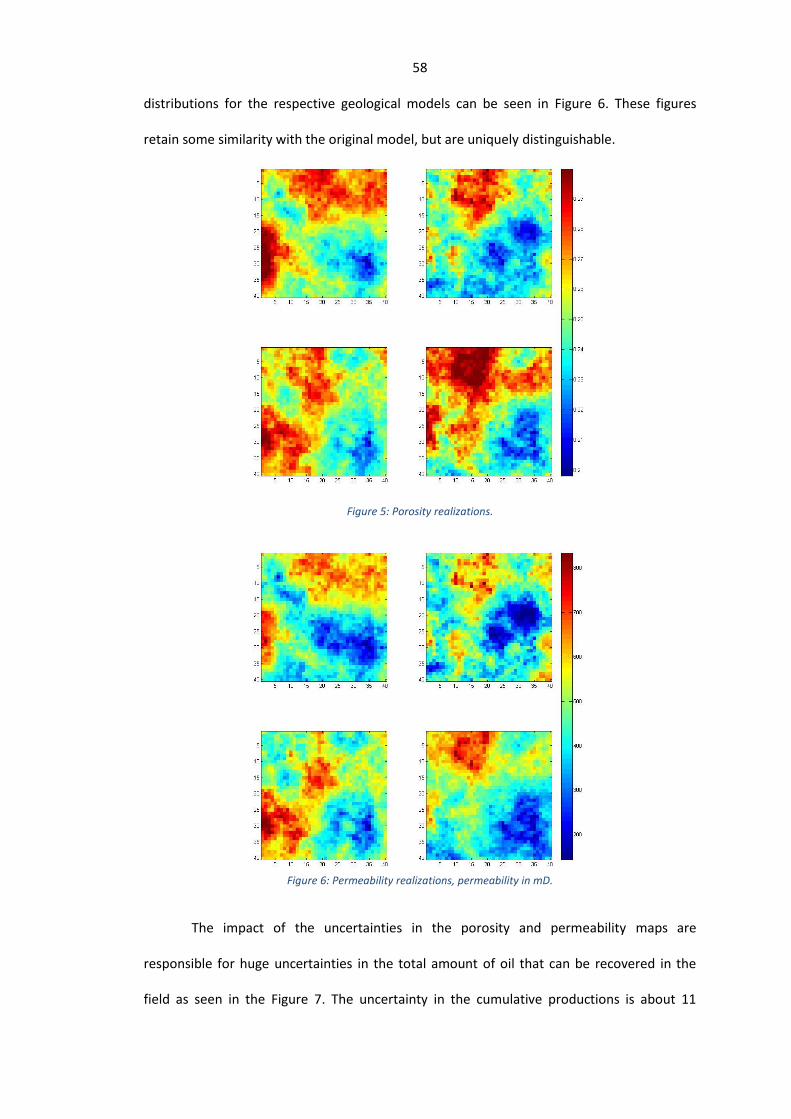
58
distributions for the respective geological models can be seen in Figure 6. These figures
retain some similarity with the original model, but are uniquely distinguishable.
Figure 5: Porosity realizations.
Figure 6: Permeability realizations, permeability in mD.
The impact of the uncertainties in the porosity and permeability maps are
responsible for huge uncertainties in the total amount of oil that can be recovered in the
field as seen in the Figure 7. The uncertainty in the cumulative productions is about 11
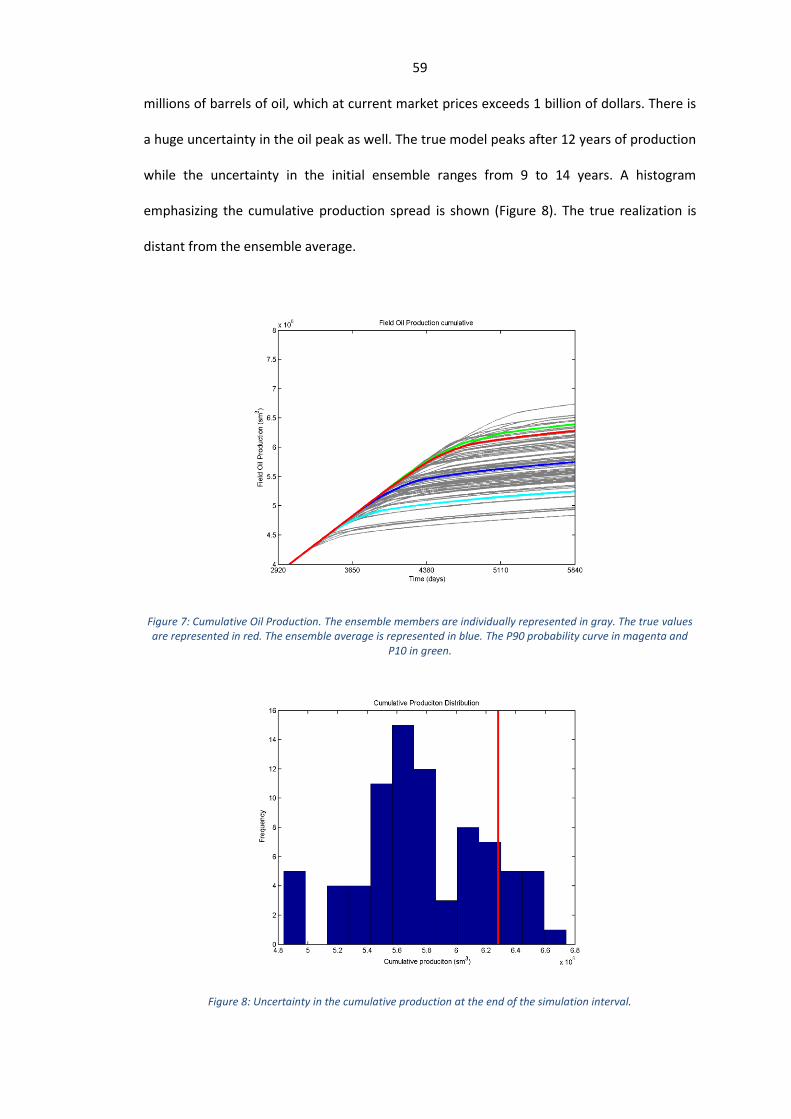
59
millions of barrels of oil, which at current market prices exceeds 1 billion of dollars. There is
a huge uncertainty in the oil peak as well. The true model peaks after 12 years of production
while the uncertainty in the initial ensemble ranges from 9 to 14 years. A histogram
emphasizing the cumulative production spread is shown (Figure 8). The true realization is
distant from the ensemble average.
Figure 7: Cumulative Oil Production. The ensemble members are individually represented in gray. The true values are represented in red. The ensemble average is represented in blue. The P90 probability curve in magenta and
P10 in green.
Figure 8: Uncertainty in the cumulative production at the end of the simulation interval.

60
The primary objective of this study is to predict with reasonable antecedence the
best moment to stop production and decommission the field before the production drops
substantially (oil peak). The objective behind this decision is to avoid economic losses due to
a late management response. Planning ahead of time is critical to reduce operational costs.
The P90 cumulative curve represents the situation in which we are 90% confident
that at least a certain production level will be reached. This confidence curve is widely used
by the oil industry to delineate proven reserves. It peaks by the end of the 10th year of
production. Thus a decision regarding future activities in the field must be planned before
this deadline.
Abandoning the field prematurely can lead to a loss of millions of dollars. On the
other side waiting too much to decommission the field will also have economical
implications. This difference is substantial and requires further uncertainty reduction. To do
this data assimilation is required.
4.4 Data Assimilation
To provide better estimates of porosity and permeability the initial ensemble
created previously was conditioned with historical data. This was done using the Ensemble
Kalman filter. Porosity, permeability, saturation and pressure were included in the state
vector. Porosity and permeability are static variables while pressure and saturation are
dynamic (produced by the reservoir simulator in runtime). The data assimilated consist of
production and seismic data obtained from the original model perturbed with Gaussian
errors.
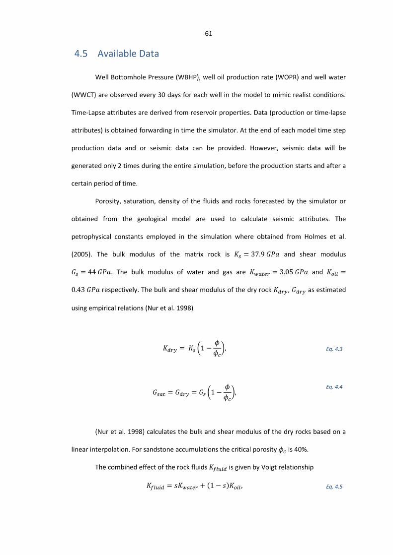
61
4.5 Available Data
Well Bottomhole Pressure (WBHP), well oil production rate (WOPR) and well water
(WWCT) are observed every 30 days for each well in the model to mimic realist conditions.
Time-Lapse attributes are derived from reservoir properties. Data (production or time-lapse
attributes) is obtained forwarding in time the simulator. At the end of each model time step
production data and or seismic data can be provided. However, seismic data will be
generated only 2 times during the entire simulation, before the production starts and after a
certain period of time.
Porosity, saturation, density of the fluids and rocks forecasted by the simulator or
obtained from the geological model are used to calculate seismic attributes. The
petrophysical constants employed in the simulation where obtained from Holmes et al.
(2005). The bulk modulus of the matrix rock is and shear modulus
. The bulk modulus of water and gas are and
respectively. The bulk and shear modulus of the dry rock , as estimated
using empirical relations (Nur et al. 1998)
(
) Eq. 4.3
(
)
Eq. 4.4
(Nur et al. 1998) calculates the bulk and shear modulus of the dry rocks based on a
linear interpolation. For sandstone accumulations the critical porosity is 40%.
The combined effect of the rock fluids is given by Voigt relationship
( ) Eq. 4.5

62
The density of the sandstone rock matrix is , the densities of
oil and water are respectively and
.
The pressure dependence is not included in these relationships, it is assumed not to
vary significantly along the reservoir life due to the voidage replacement recovery process
being used to produce this reservoir. The initial pressure is 30 MPa.
4.6 Measurement Errors
WBHP, WOPR and WWCT observations are perturbed with noise. The production
measurement errors are drawn from a Gaussian distribution with a mean zero and standard
deviation as specified:
• Oil production rate (OPR): 5%
• Bottom hole pressure (BHP): 6%
• Water cut (WCT): 7%
This setup follows the usual amount of uncertainty found in the industry. Oil
production rates are usually well known, while bottomhole pressures are known with lower
accuracy and water cut with even lower.
To incorporate time-lapse attributes in this study under realistic conditions a
sensitivity test will be performed to verify the impact of the quality of the data (confidence)
on the study. The error will be taken as a percentage of the time-lapse signal observed.
4.7 Objectives and Analysis of the Results
The objective to this study is to reduce uncertainties in the production forecast and
to predict the oil peak. This objective will be evaluated by measuring the ensemble spread in
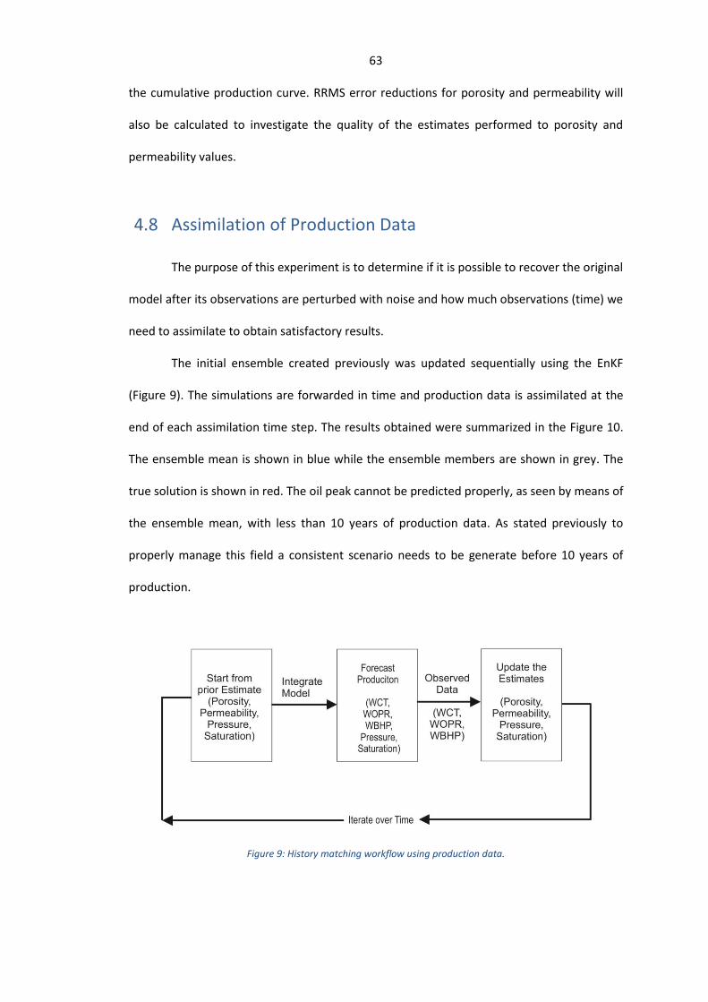
63
the cumulative production curve. RRMS error reductions for porosity and permeability will
also be calculated to investigate the quality of the estimates performed to porosity and
permeability values.
4.8 Assimilation of Production Data
The purpose of this experiment is to determine if it is possible to recover the original
model after its observations are perturbed with noise and how much observations (time) we
need to assimilate to obtain satisfactory results.
The initial ensemble created previously was updated sequentially using the EnKF
(Figure 9). The simulations are forwarded in time and production data is assimilated at the
end of each assimilation time step. The results obtained were summarized in the Figure 10.
The ensemble mean is shown in blue while the ensemble members are shown in grey. The
true solution is shown in red. The oil peak cannot be predicted properly, as seen by means of
the ensemble mean, with less than 10 years of production data. As stated previously to
properly manage this field a consistent scenario needs to be generate before 10 years of
production.
Figure 9: History matching workflow using production data.
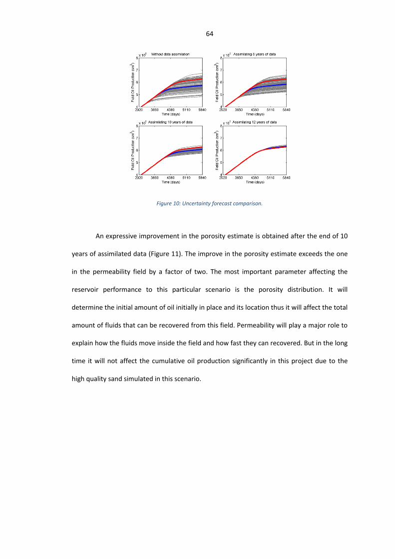
64
Figure 10: Uncertainty forecast comparison.
An expressive improvement in the porosity estimate is obtained after the end of 10
years of assimilated data (Figure 11). The improve in the porosity estimate exceeds the one
in the permeability field by a factor of two. The most important parameter affecting the
reservoir performance to this particular scenario is the porosity distribution. It will
determine the initial amount of oil initially in place and its location thus it will affect the total
amount of fluids that can be recovered from this field. Permeability will play a major role to
explain how the fluids move inside the field and how fast they can recovered. But in the long
time it will not affect the cumulative oil production significantly in this project due to the
high quality sand simulated in this scenario.

65
Figure 11: RRMS error after 12 years of production for porosity and permeability.
The evolution of the estimates in time is presented (Figure 12 and Figure 13). The
results can be compared with the true permeability and porosity fields (Figure 2). As
previously observed in the RRMS reduction plot (Figure 11) the updates are more significant
after 10 years of historical production.
To reduce this decision time the use of time-lapse data becomes an alternative.
Simulations making use of production and seismic data to help constrain the flow were
performed in the upcoming section.
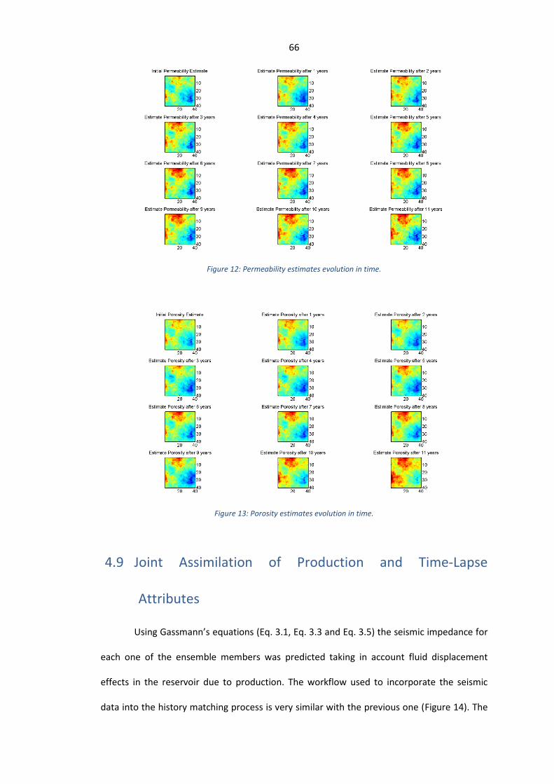
66
Figure 12: Permeability estimates evolution in time.
Figure 13: Porosity estimates evolution in time.
4.9 Joint Assimilation of Production and Time-Lapse
Attributes
Using Gassmann’s equations (Eq. 3.1, Eq. 3.3 and Eq. 3.5) the seismic impedance for
each one of the ensemble members was predicted taking in account fluid displacement
effects in the reservoir due to production. The workflow used to incorporate the seismic
data into the history matching process is very similar with the previous one (Figure 14). The
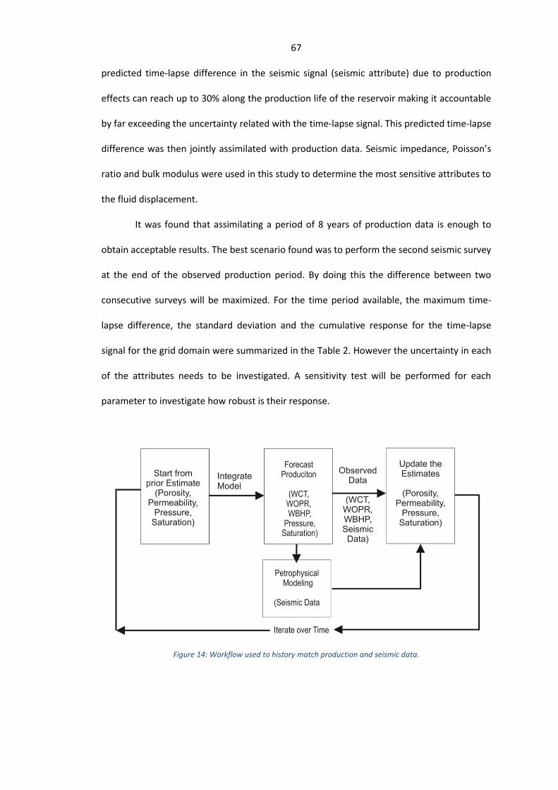
67
predicted time-lapse difference in the seismic signal (seismic attribute) due to production
effects can reach up to 30% along the production life of the reservoir making it accountable
by far exceeding the uncertainty related with the time-lapse signal. This predicted time-lapse
difference was then jointly assimilated with production data. Seismic impedance, Poisson’s
ratio and bulk modulus were used in this study to determine the most sensitive attributes to
the fluid displacement.
It was found that assimilating a period of 8 years of production data is enough to
obtain acceptable results. The best scenario found was to perform the second seismic survey
at the end of the observed production period. By doing this the difference between two
consecutive surveys will be maximized. For the time period available, the maximum time-
lapse difference, the standard deviation and the cumulative response for the time-lapse
signal for the grid domain were summarized in the Table 2. However the uncertainty in each
of the attributes needs to be investigated. A sensitivity test will be performed for each
parameter to investigate how robust is their response.
Figure 14: Workflow used to history match production and seismic data.

68
Attribute Max
Variation (%)
Standard
deviation (%)
Cumulative
Response (%)
3.45 1.09 2218
13.90 4.39 8840
31.25 10.41 21588
Table 2: Seismic attribute time-lapse response after 8 years of production.
4.9.1 Seismic Impedance Results
The first attribute tested was the seismic impedance. The time-lapse seismic signal
was perturbed with Gaussian errors with zero mean and standard deviation of 2% of the
signal (time-lapse difference). The assimilation results are shown in Figure 15. A significant
improvement in the quality of the estimates is obtained by the joint assimilation of
production and seismic data. The estimated permeability and porosity fields evolution in
time can be seen in the Figure 16 and Figure 17. The difference obtained by the assimilation
of time-lapse seismic impedance is notable. The field shapes change significantly and recover
the shape of the original ones (Figure 2). The improvements in the estimate are significant
and can be summarized in the Table 3. A graphical representation of its evolution in time is
also provided (Figure 18).

69
Figure 15: Comparison between the results obtained assimilating only production data against the joint assimilation of production and seismic impedance data.
Time since base
survey (years)
Porosity estimate
improvement (%)
Permeability
estimate
improvement (%)
4 46.93 20.48
6 52.40 24.42
8 55.73 20.42
Table 3: Porosity and permeability estimates improvement due to the use of Time-Lapse seismic impedance data.
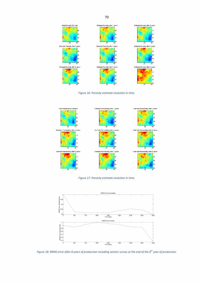
70
Figure 16: Porosity estimate evolution in time.
Figure 17: Porosity estimate evolution in time.
Figure 18: RRMS error after 8 years of production including seismic survey at the end of the 8th
year of production.
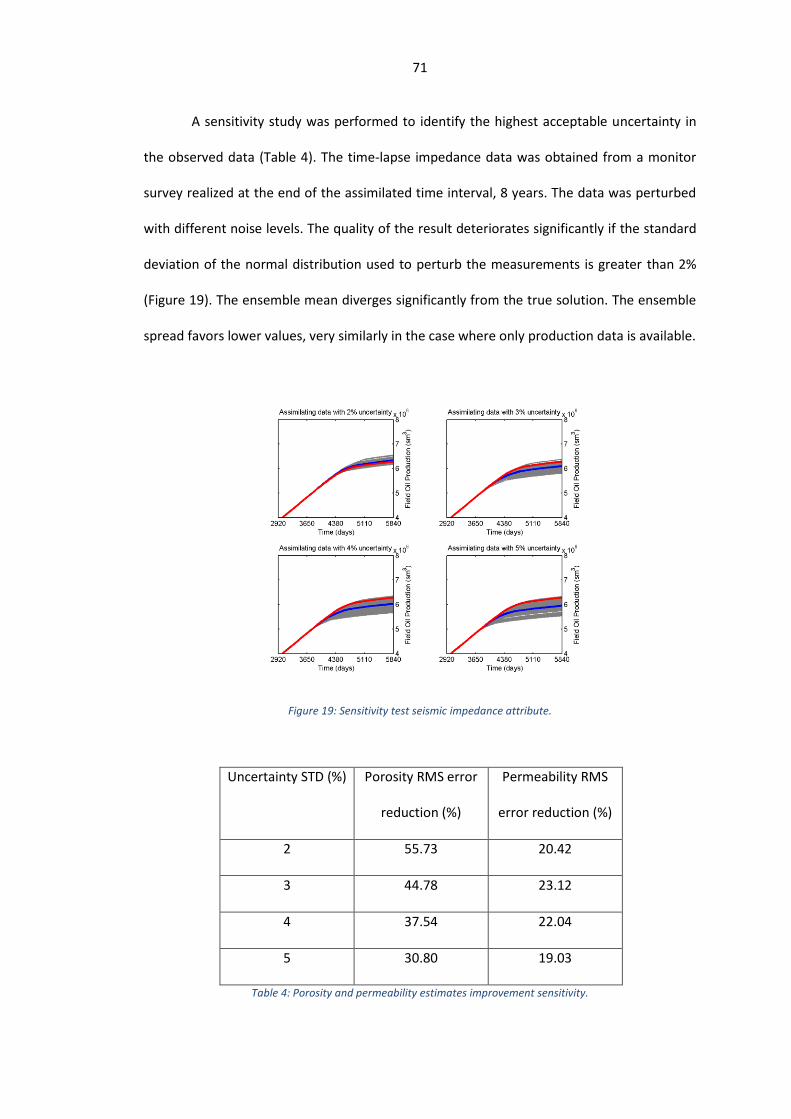
71
A sensitivity study was performed to identify the highest acceptable uncertainty in
the observed data (Table 4). The time-lapse impedance data was obtained from a monitor
survey realized at the end of the assimilated time interval, 8 years. The data was perturbed
with different noise levels. The quality of the result deteriorates significantly if the standard
deviation of the normal distribution used to perturb the measurements is greater than 2%
(Figure 19). The ensemble mean diverges significantly from the true solution. The ensemble
spread favors lower values, very similarly in the case where only production data is available.
Figure 19: Sensitivity test seismic impedance attribute.
Uncertainty STD (%) Porosity RMS error
reduction (%)
Permeability RMS
error reduction (%)
2 55.73 20.42
3 44.78 23.12
4 37.54 22.04
5 30.80 19.03
Table 4: Porosity and permeability estimates improvement sensitivity.
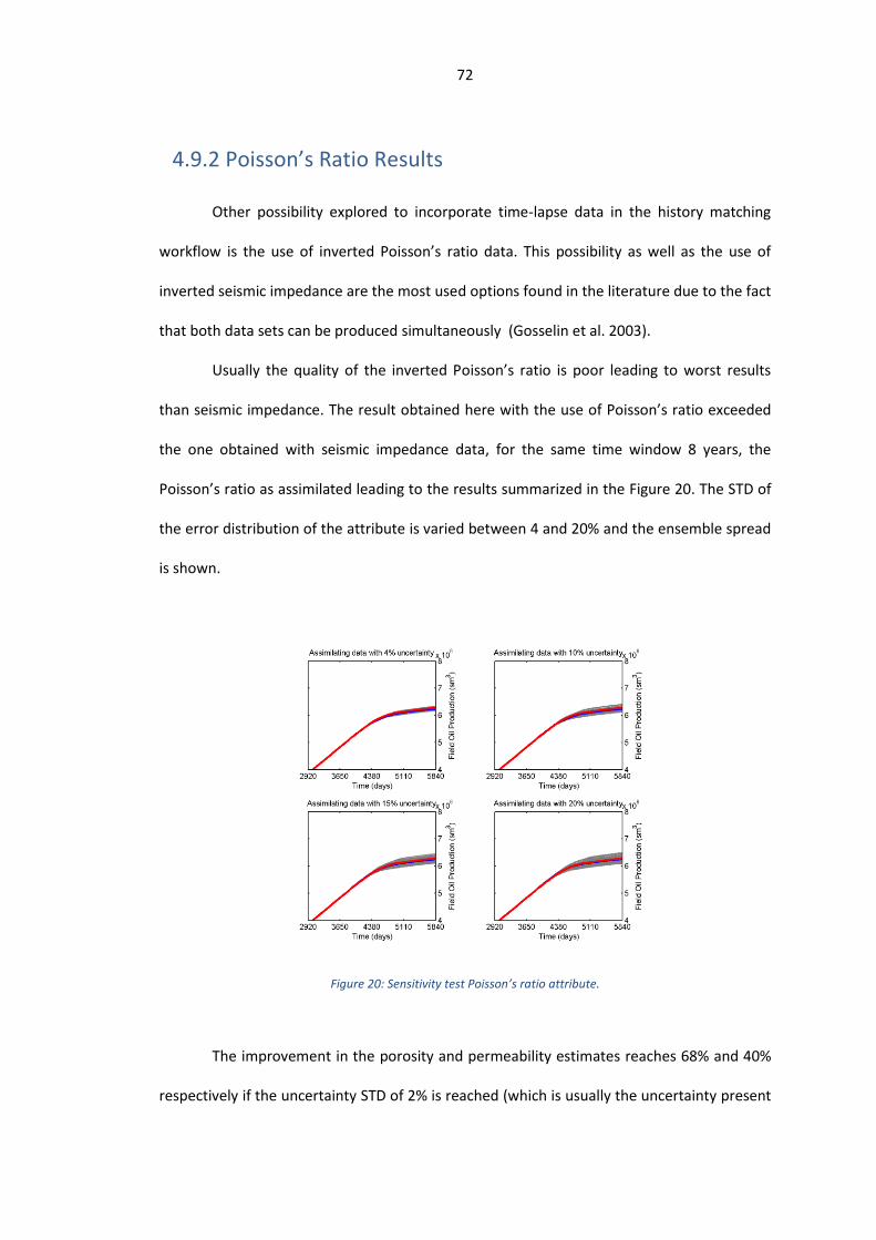
72
4.9.2 Poisson’s Ratio Results
Other possibility explored to incorporate time-lapse data in the history matching
workflow is the use of inverted Poisson’s ratio data. This possibility as well as the use of
inverted seismic impedance are the most used options found in the literature due to the fact
that both data sets can be produced simultaneously (Gosselin et al. 2003).
Usually the quality of the inverted Poisson’s ratio is poor leading to worst results
than seismic impedance. The result obtained here with the use of Poisson’s ratio exceeded
the one obtained with seismic impedance data, for the same time window 8 years, the
Poisson’s ratio as assimilated leading to the results summarized in the Figure 20. The STD of
the error distribution of the attribute is varied between 4 and 20% and the ensemble spread
is shown.
Figure 20: Sensitivity test Poisson’s ratio attribute.
The improvement in the porosity and permeability estimates reaches 68% and 40%
respectively if the uncertainty STD of 2% is reached (which is usually the uncertainty present
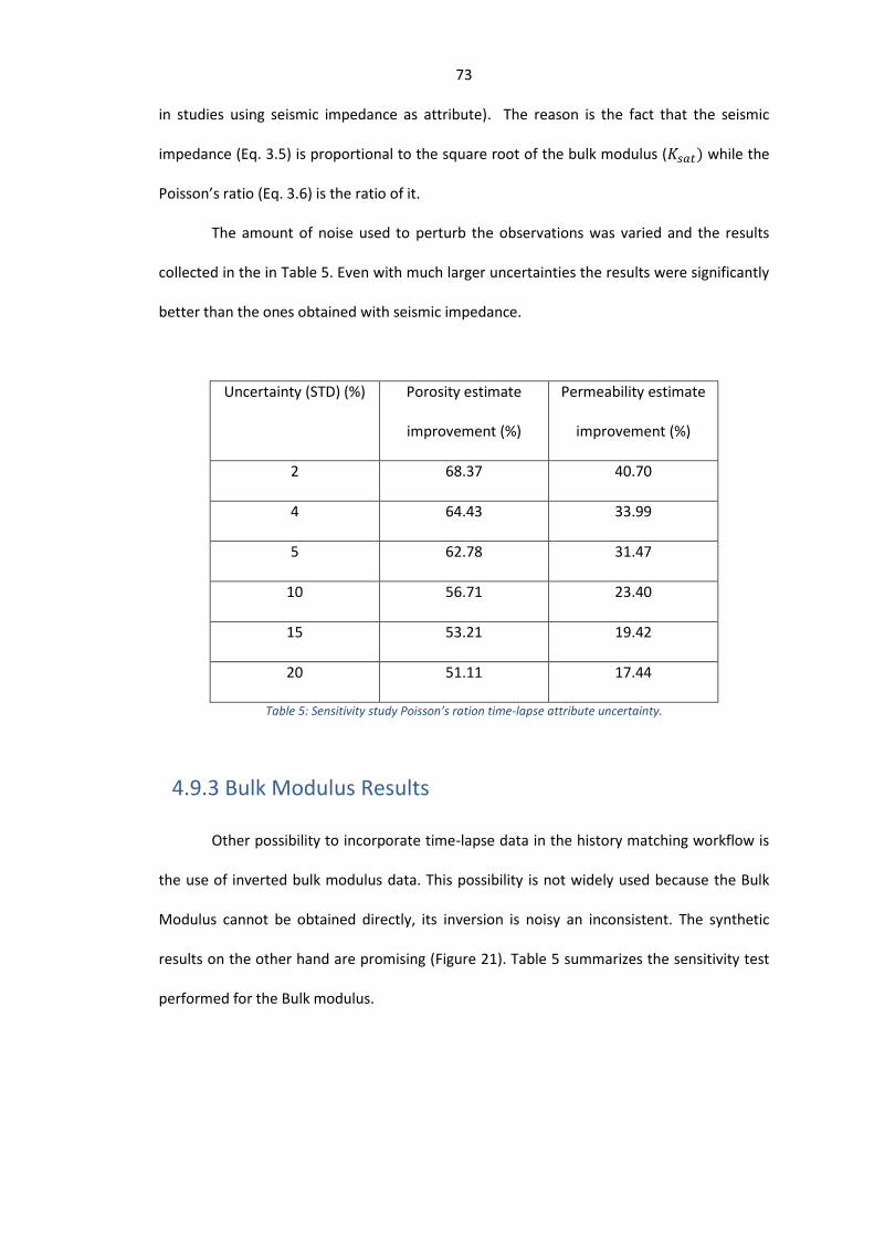
73
in studies using seismic impedance as attribute). The reason is the fact that the seismic
impedance (Eq. 3.5) is proportional to the square root of the bulk modulus ( ) while the
Poisson’s ratio (Eq. 3.6) is the ratio of it.
The amount of noise used to perturb the observations was varied and the results
collected in the in Table 5. Even with much larger uncertainties the results were significantly
better than the ones obtained with seismic impedance.
Uncertainty (STD) (%) Porosity estimate
improvement (%)
Permeability estimate
improvement (%)
2 68.37 40.70
4 64.43 33.99
5 62.78 31.47
10 56.71 23.40
15 53.21 19.42
20 51.11 17.44
Table 5: Sensitivity study Poisson’s ration time-lapse attribute uncertainty.
4.9.3 Bulk Modulus Results
Other possibility to incorporate time-lapse data in the history matching workflow is
the use of inverted bulk modulus data. This possibility is not widely used because the Bulk
Modulus cannot be obtained directly, its inversion is noisy an inconsistent. The synthetic
results on the other hand are promising (Figure 21). Table 5 summarizes the sensitivity test
performed for the Bulk modulus.
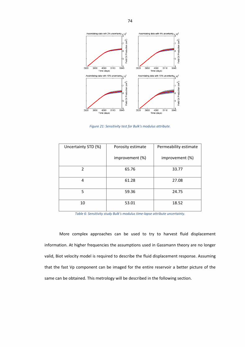
74
Figure 21: Sensitivity test for Bulk's modulus attribute.
Uncertainty STD (%) Porosity estimate
improvement (%)
Permeability estimate
improvement (%)
2 65.76 33.77
4 61.28 27.08
5 59.36 24.75
10 53.01 18.52
Table 6: Sensitivity study Bulk’s modulus time-lapse attribute uncertainty.
More complex approaches can be used to try to harvest fluid displacement
information. At higher frequencies the assumptions used in Gassmann theory are no longer
valid, Biot velocity model is required to describe the fluid displacement response. Assuming
that the fast Vp component can be imaged for the entire reservoir a better picture of the
same can be obtained. This metrology will be described in the following section.
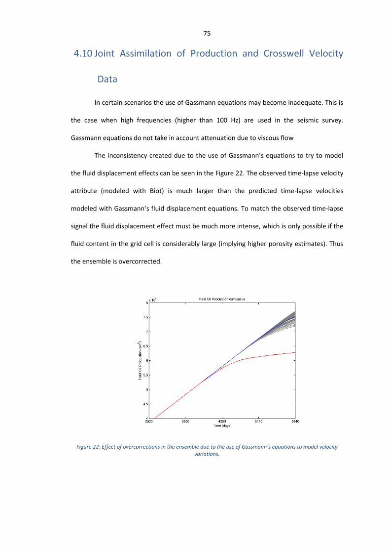
75
4.10 Joint Assimilation of Production and Crosswell Velocity
Data
In certain scenarios the use of Gassmann equations may become inadequate. This is
the case when high frequencies (higher than 100 Hz) are used in the seismic survey.
Gassmann equations do not take in account attenuation due to viscous flow
The inconsistency created due to the use of Gassmann’s equations to try to model
the fluid displacement effects can be seen in the Figure 22. The observed time-lapse velocity
attribute (modeled with Biot) is much larger than the predicted time-lapse velocities
modeled with Gassmann’s fluid displacement equations. To match the observed time-lapse
signal the fluid displacement effect must be much more intense, which is only possible if the
fluid content in the grid cell is considerably large (implying higher porosity estimates). Thus
the ensemble is overcorrected.
Figure 22: Effect of overcorrections in the ensemble due to the use of Gassmann’s equations to model velocity variations.

76
To overcome this limitation a new petrophysical model is required. (Biot 1956)
addressed this problem. In Biot’s formulation 3 velocity components are present. The fast
velocity component can be easily obtained from a seismic tomography avoiding the need to
invert the data (seismic inversion). The fast velocity component which sensitive to fluid
displacement and can used as time-lapse data attribute.
However imaging at such frequencies is impossible in a real field scenario. A possible
way to try to take advantage of such methodology is through the use of crosswell data. The
source frequencies used for such surveys can be much bigger than the ones used in surface
seismic.
A potentially unexplored approach is the used of crosswell tomography to map the
fluid changes in the reservoir. This approach has several advantages over conventional time-
lapse seismic acquisitions. The most important one it the cost to obtain the data. Running a
full field survey is several times more expensive than collecting data only at certain
locations, reproducibility is also a major issue. Reproducing the acquisition setup of the base
survey is challenging and can severely compromise the quality of the time-lapse data
obtained. The advantage of using wells as fixed points to collect data easies this
requirement. Another potential advantage is the use of high frequencies to image the
interwell region, which leads to higher spatial resolution. Higher frequencies can also
highlight the fluid displacement effect easier. The uncertainties in the data are much
smaller. The use of crosswell tomography can provide a velocity map directly which then can
be modeled using the Biot velocity model. The major disadvantage is the limited area
coverage of the method.
Two acquisition configurations were used (Figure 23). In the first configuration time-
lapse data is acquired between all the wells, while in the second configuration data is only
acquired between injector and producers. The slow component has a good sensitivity to
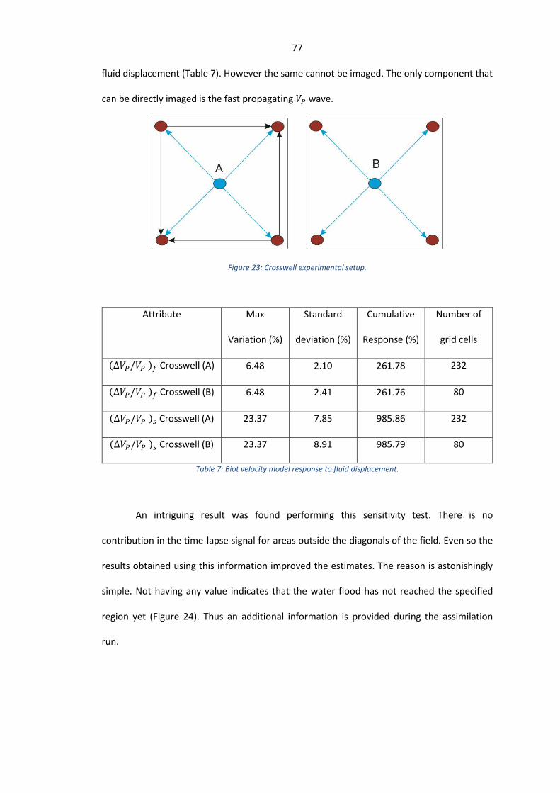
77
fluid displacement (Table 7). However the same cannot be imaged. The only component that
can be directly imaged is the fast propagating wave.
Figure 23: Crosswell experimental setup.
Attribute Max
Variation (%)
Standard
deviation (%)
Cumulative
Response (%)
Number of
grid cells
( ) Crosswell (A) 6.48 2.10 261.78 232
( ) Crosswell (B) 6.48 2.41 261.76 80
( ) Crosswell (A) 23.37 7.85 985.86 232
( ) Crosswell (B) 23.37 8.91 985.79 80
Table 7: Biot velocity model response to fluid displacement.
An intriguing result was found performing this sensitivity test. There is no
contribution in the time-lapse signal for areas outside the diagonals of the field. Even so the
results obtained using this information improved the estimates. The reason is astonishingly
simple. Not having any value indicates that the water flood has not reached the specified
region yet (Figure 24). Thus an additional information is provided during the assimilation
run.
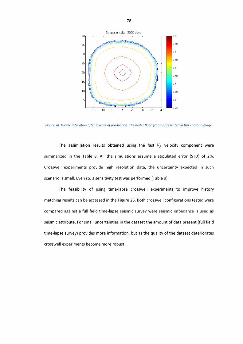
78
Figure 24: Water saturation after 8 years of production. The water flood front is presented in this contour image.
The assimilation results obtained using the fast velocity component were
summarized in the Table 8. All the simulations assume a stipulated error (STD) of 2%.
Crosswell experiments provide high resolution data, the uncertainty expected in such
scenario is small. Even so, a sensitivity test was performed (Table 9).
The feasibility of using time-lapse crosswell experiments to improve history
matching results can be accessed in the Figure 25. Both crosswell configurations tested were
compared against a full field time-lapse seismic survey were seismic impedance is used as
seismic attribute. For small uncertainties in the dataset the amount of data present (full field
time-lapse survey) provides more information, but as the quality of the dataset deteriorates
crosswell experiments become more robust.
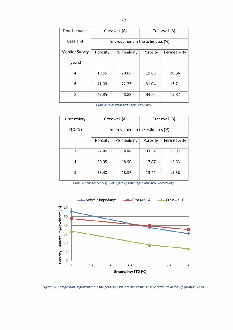
79
Time between
Base and
Monitor Survey
(years)
Crosswell (A) Crosswell (B)
Improvement in the estimates (%)
Porosity Permeability Porosity Permeability
4 19.65 20.66 19.65 20.66
6 41.09 22.77 31.04 16.71
8 47.85 18.88 33.52 15.87
Table 8: RMS error reduction summary.
Uncertainty
STD (%)
Crosswell (A) Crosswell (B)
Improvement in the estimates (%)
Porosity Permeability Porosity Permeability
2 47.85 18.88 33.52 15.87
4 39.35 18.50 17.87 15.63
5 35.40 18.57 13.44 15.56
Table 9: Sensitivity study Biot’s fast Vp time-lapse attribute uncertainty.
Figure 25: Comparison improvement in the porosity estimate due to the seismic attribute and configuration used.
0
10
20
30
40
50
60
2 2.5 3 3.5 4 4.5 5
Po
rosi
ty E
stim
ate
Im
pro
vem
en
t (%
)
Uncertainty STD (%)
Seismic Impedance Crosswell A Crosswell B
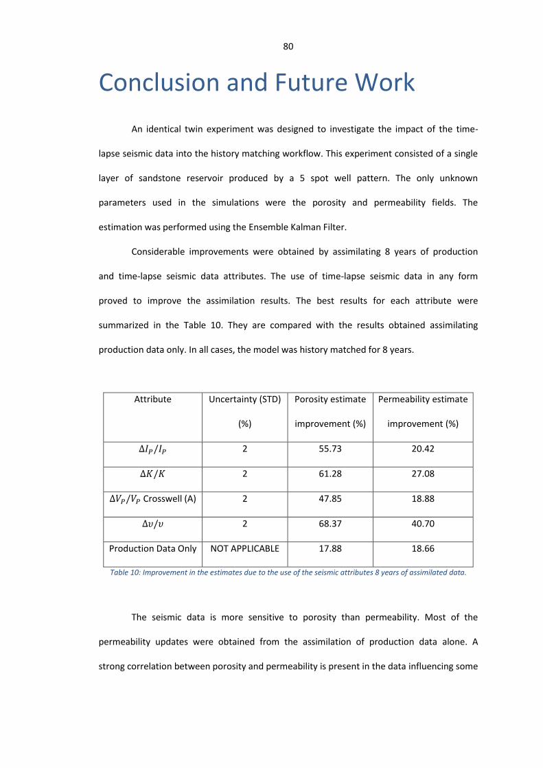
80
Conclusion and Future Work
An identical twin experiment was designed to investigate the impact of the time-
lapse seismic data into the history matching workflow. This experiment consisted of a single
layer of sandstone reservoir produced by a 5 spot well pattern. The only unknown
parameters used in the simulations were the porosity and permeability fields. The
estimation was performed using the Ensemble Kalman Filter.
Considerable improvements were obtained by assimilating 8 years of production
and time-lapse seismic data attributes. The use of time-lapse seismic data in any form
proved to improve the assimilation results. The best results for each attribute were
summarized in the Table 10. They are compared with the results obtained assimilating
production data only. In all cases, the model was history matched for 8 years.
Attribute Uncertainty (STD)
(%)
Porosity estimate
improvement (%)
Permeability estimate
improvement (%)
2 55.73 20.42
2 61.28 27.08
Crosswell (A) 2 47.85 18.88
2 68.37 40.70
Production Data Only NOT APPLICABLE 17.88 18.66
Table 10: Improvement in the estimates due to the use of the seismic attributes 8 years of assimilated data.
The seismic data is more sensitive to porosity than permeability. Most of the
permeability updates were obtained from the assimilation of production data alone. A
strong correlation between porosity and permeability is present in the data influencing some

81
updates. The assimilation of Poisson’s ratio and bulk modulus attributes significantly
improved the permeability estimate (for the cases with small error in the data).
Some of the attributes compared here cannot be obtained directly, their acquisition
is difficult and unreliable. In a real case application the use of these attributes is not
recommended. The most used attributes in practice are the seismic impedance and
Poisson’s ratio. Velocity fields and bulk modulus are not used due to the previous fact.
Among these attributes, Poisson’s ratio demonstrated to be the most sensitive to fluid
displacement. In practical applications however the use of this attribute is usually avoided
due to poor quality of the data. This may be a point of further improvements for real
applications, obtaining reliable Poisson’s ratio time-lapse data can boost history matching
results significantly. The result obtained with crosswell tomography was impressive given
the amount of data available (data is only available in the interwell region).
The use of crosswell data can be extremely beneficial as a time-lapse tool because of
its lower cost and higher reproducibility when compared to conventional surface seismic
surveys. The fast component of the velocity field is more sensitive to fluid displacement.
It can only be observed at higher frequencies (which is the case for crosswell applications).
The major disadvantage on the other side is the lower area coverage of this technique. The
use of crosswell data provides data along a plane and cannot be directly extended to the
entire volume of the grid cell. Methods to upscale the imaged velocities to an entire volume
need to be further studied. More realistic applications are required to further evaluate this
technique. Reservoir applications are much more complex, faults and other complex
geological features will determine the applicability of this method.
This is still an ongoing project which aims to integrate into a single assimilation loop
every possible data source available among then gravity data, surface seismic data, crosswell
data, VSP data, electromagnetic and production data.

82
Last but not least important, avoiding the use of seismic data attributes (which
requires seismic inversion) harvesting information directly from the seismic waves can bring
major benefits to the assimilation workflow. This procedure is highly non-linear and
challenging, but it avoids the uncertainties generated due to the inversion process.

83
REFERENCES
1. Aanonsen, S. I., G. Naevdal, et al. (2009). "The Ensemble Kalman Filter in Reservoir Engineering-a Review." Spe Journal 14(3): 393-412.
2. Abubakar, A., T. Habashy, et al. (2013). Joint inversion of time-lapse crosswell seismic and production data for reservoir monitoring and characterization. 6th International Petroleum Technology Conference.
3. Agbalaka, C. C. and D. S. Oliver (2008). "Application of the EnKF and localization to automatic history matching of facies distribution and production data." Mathematical Geosciences 40(4): 353-374.
4. Aid, K. and P. Richards (1980). "Quantitative seismology: theory and methods." San Francisco.
5. Bianco, A., A. Cominelli, et al. (2007). History Matching and Production Forecast Uncertainty by Means of the Ensemble Kalman Filter: A Real Field Application. EUROPEC/EAGE Conference and Exhibition. London, U.K., Society of Petroleum Engineers.
6. Biot, M. A. (1956). "Theory of propagation of elastic waves in a fluid‐saturated porous solid. I. Low‐frequency range." The Journal of the Acoustical Society of America 28: 168.
7. Chen, Y. and D. S. Oliver (2009a). Ensemble-Based Closed-Loop Optimization Applied to Brugge Field. SPE Reservoir Simulation Symposium. The Woodlands, Texas, USA, Society of Petroleum Engineers.
8. Chen, Y., D. S. Oliver, et al. (2009b). "Data assimilation for nonlinear problems by ensemble Kalman filter with reparameterization." Journal of Petroleum Science and Engineering 66(1-2): 1-14.
9. Commission, E. (2006). "World Energy Technology Outlook 2050–WETO H2." Office for Official Publications of the European Communities, Brüssel.
10. Dadashpour, M., D. Echeverría-Ciaurri, et al. (2009). "Porosity and permeability estimation by integration of production and time-lapse near and far offset seismic data." Journal of Geophysics and Engineering 6(4): 325.
11. Dadashpour, M., M. Landrø, et al. (2008). "Nonlinear inversion for estimating reservoir parameters from time-lapse seismic data." Journal of Geophysics and Engineering 5(1): 54
12. Devegowda, D., E. Arroyo, et al. (2007). Efficient and Robust Reservoir Model Updating Using Ensemble Kalman Filter With Sensitivity-Based Covariance Localization. SPE Reservoir Simulation Symposium. Houston, Texas, U.S.A., Society of Petroleum Engineers.
84
13. Dijkstra, T. and T. Oldenziel (2003). Time-lapse Seismic Within Reservoir Engineering, Technische Universiteit Delft.
14. Domenico, S. (1976). "Effect of brine-gas mixture on velocity in an unconsolidated sand reservoir." Geophysics 41(5): 882-894.
15. Dong, Y., Y. Gu, et al. (2006). "Sequential assimilation of 4D seismic data for reservoir description using the ensemble Kalman filter." Journal of Petroleum Science and Engineering 53(1-2): 83-99.
16. Doren, J. V., G. V. Essen, et al. (2012). A Comprehensive Workflow for Assisted History Matching Applied to a Complex Mature Reservoir. SPE Europec/EAGE Annual Conference. Copenhagen, Denmark, Society of Petroleum Engineers.
17. Droujinina, A., C. MacBeth, et al. (2001). Time-lapse crosswell tomography in the Athabasca Tar Sands. 2001 SEG Annual Meeting.
18. Dudley, B. (2012). "BP statistical review of world energy." from http://www.bp.com/assets/bp_internet/globalbp/globalbp_uk_english/reports_and_publications/statistical_energy_review_2011/STAGING/local_assets/pdf/statistical_review_of_world_energy_full_report_2012.pdf.
19. Emerick, A. A. (2012). HISTORY MATCHING AND UNCERTAINTY CHARACTERIZATION USING ENSEMBLE-BASED METHODS, The University of Tulsa.
20. Emerick, A. A. and A. C. Reynolds (2012). "History matching time-lapse seismic data using the ensemble Kalman filter with multiple data assimilations." Computational Geosciences 16(3): 639-659.
21. Evensen, G. (2004). "Sampling strategies and square root analysis schemes for the EnKF." Ocean Dynamics 54(6): 539-560.
22. Fahimuddin, A., S. I. Aanonsen, et al. (2010). Ensemble Based 4D Seismic History Matching: Integration of Different Levels and Types of Seismic Data. SPE EUROPEC/EAGE Annual Conference and Exhibition. Barcelona, Spain, Society of Petroleum Engineers.
23. Gao, G., M. Zafari, et al. (2006). "Quantifying uncertainty for the PUNQ-S3 problem in a Bayesian setting with RML and EnKF." Spe Journal 11(4): 506-515.
24. Gaspari, G. and S. E. Cohn (1999). "Construction of correlation functions in two and three dimensions." Quarterly Journal of the Royal Meteorological Society 125(554): 723-757.
25. Gassmann, F. (1951). Über die elastizität poröser medien, Inst. für Geophysik an der ETH.
26. Geertsma, J. and D. Smit (1961). "Some aspects of elastic wave propagation in fluid-saturated porous solids." Geophysics 26(2): 169-181.
27. Gosselin, O., S. I. Aanonsen, et al. (2003). History Matching Using Time-lapse Seismic (HUTS). SPE Annual Technical Conference and Exhibition. Denver, Colorado, Society of Petroleum Engineers.

85
28. Gosselin, O., S. van den Berg, et al. (2001). Integrated history-matching of production and 4D seismic data. SPE Annual Technical Conference and Exhibition.
29. Gu, Y. and D. S. Oliver (2004). History Matching of the PUNQ-S3 Reservoir Model Using the Ensemble Kalman Filter. SPE Annual Technical Conference and Exhibition. Houston, Texas, Society of Petroleum Engineers.
30. Gu, Y. and D. S. Oliver (2005a). "History Matching of the PUNQ-S3 Reservoir Model Using the Ensemble Kalman Filter." Spe Journal 10(2): pp. 217-224.
31. Gu, Y. and D. S. Oliver (2007). "An iterative ensemble Kalman filter for multiphase fluid flow data assimilation." Spe Journal 12(4): 438-446.
32. Gu, Y. Q. and D. S. Oliver (2005b). "History matching of the PUNQ-S3 reservoir model using the ensemble Kalman filter." Spe Journal 10(2): 217-224.
33. Gu, Y. Q. and D. S. Oliver (2006). "The ensemble Kalman filter for continuous updating of reservoir simulation models." Journal of Energy Resources Technology-Transactions of the Asme 128(1): 79-87.
34. Han, D.-h. and M. L. Batzle (2004). "Gassmann's equation and fluid-saturation effects on seismic velocities." Geophysics 69(2): 398-405.
35. Hanea, R. G., J. K. Przybysz-jarnut, et al. (2010). The Choice of a ‘Best’ Assisted History Matching Algorithm. SPE EUROPEC/EAGE Annual Conference and Exhibition. Barcelona, Spain, Society of Petroleum Engineers.
36. Haugen, V., G. Naevdal, et al. (2008). "History Matching Using the Ensemble Kalman Filter on a North Sea Field Case." Spe Journal 13(4): 382-391.
37. Holmes, M. and A. Holmes (2005). Petrophysical rock physics modeling: a comparison of the Krief and Gassmann equations, and applications to verifying and estimating compressional and shear velocities: Presented at the 46thAnnual Logging Symposium. SPWLA 46th Annual Logging Symposium, New Orleans: Society of Petroleum Well Log Analysts.
38. Houtekamer, P. L. and H. L. Mitchell (2001). "A Sequential Ensemble Kalman Filter for Atmospheric Data Assimilation." Monthly Weather Review 129(1): 123-137.
39. Jafarpour, B. and D. B. McLaughlin (2009). "Estimating Channelized-Reservoir Permeabilities With the Ensemble Kalman Filter: The Importance of Ensemble Design." Spe Journal 14(2): 374-388.
40. Jin, L., G. Tiller, et al. (2011). An Integrated Workflow for Quantitative 4D Seismic Data Integration: A Case Study. International Petroleum Technology Conference. Bangkok, Thailand, International Petroleum Technology Conference.
41. Johnson, D. L., J. Koplik, et al. (1987). "Theory of dynamic permeability and tortuosity in fluid-saturated porous media." Journal of fluid mechanics 176(1): 379-402.
86
42. Landa, J. L. and D. Kumar (2011). Joint Inversion of 4D Seismic and Production Data. SPE Annual Technical Conference and Exhibition. Denver, Colorado, USA, Society of Petroleum Engineers.
43. Leeuwenburgh, O., J. Brouwer, et al. (2011a). "Ensemble-based conditioning of reservoir models to seismic data." Computational Geosciences 15(2): 359-378.
44. Leeuwenburgh, O., P. J. P. Egberts, et al. (2010). Ensemble Methods for Reservoir Life-Cycle Optimization and Well Placement. SPE/DGS Saudi Arabia Section Technical Symposium and Exhibition. Al-Khobar, Saudi Arabia, Society of Petroleum Engineers.
45. Leeuwenburgh, O., E. Peters, et al. (2011b). Towards an Integrated Workflow for Structural Reservoir Model Updating and History Matching. SPE EUROPEC/EAGE Annual Conference and Exhibition. Vienna, Austria, Society of Petroleum Engineers.
46. Li, G. and A. C. Reynolds (2009). "Iterative Ensemble Kalman Filters for Data Assimilation." Spe Journal 14(3): 496-505.
47. Liang, B., K. Sepehrnoori, et al. (2009). "An automatic history matching module with distributed and parallel computing." Petroleum Science and Technology 27(10): 1092-1108.
48. Liang, L., A. Abubakar, et al. (2011). Improved Estimation of Permeability from Joint Inversion of Time-Lapse Crosswell Electromagnetic and Production Data Using Gradient-Based Method. SPE Annual Technical Conference and Exhibition.
49. Lie, K. A., S. Krogstad, et al. (2012). "Open-source MATLAB implementation of consistent discretisations on complex grids." Computational Geosciences 16(2): 297-322.
50. Lien, M., I. Berre, et al. (2006). "COMBINED ADAPTIVE MULTISCALE AND LEVEL-SET PARAMETER ESTIMATION." Multiscale Modeling & Simulation 4(4): 1349-1372.
51. Liu, N. and D. S. Oliver (2005). Critical Evaluation of the Ensemble Kalman Filter on History Matching of Geologic Facies. SPE Reservoir Simulation Symposium. The Woodlands, Texas, 2005,. Society of Petroleum Engineers Inc.
52. Lorentzen, R. J., K. K. Fjelde, et al. (2001). Underbalanced and Low-head Drilling Operations: Real Time Interpretation of Measured Data and Operational Support. SPE Annual Technical Conference and Exhibition. New Orleans, Louisiana, Copyright 2001, Society of Petroleum Engineers Inc.
53. Lorentzen, R. J. and G. Naevdal (2011). "An Iterative Ensemble Kalman Filter." Automatic Control, IEEE Transactions on 56(8): 1990-1995.
54. Lorentzen, R. J., G. Naevdal, et al. (2005). Analysis of the Ensemble Kalman Filter for Estimation of Permeability and Porosity in Reservoir Models. SPE Annual Technical Conference and Exhibition. Dallas, Texas, Society of Petroleum Engineers.
55. Lumley, D. E. and R. A. Behrens (1998). "Practical Issues of 4D Seismic Reservoir Monitoring: What an Engineer Needs to Know." SPE Reservoir Evaluation & Engineering 1(6): 528-538.
87
56. Maamari, A., R. Adawi, et al. (2011). "Time-lapse down-hole seismic surveys for deep EOR target monitoring in South Oman."
57. MAVKO, G., T. MUKERJI, et al. (2009). "The rock physics handbook: tools for seismic analysis of porous media."
58. Mavko, G. and R. Nolen-Hoeksema (1994). "Estimating seismic velocities at ultrasonic frequencies in partially saturated rocks." Geophysics 59(2): 252-258.
59. Murphy, W. F. (1984). "Acoustic measures of partial gas saturation in tight sandstones." Journal of Geophysical Research: Solid Earth (1978–2012) 89(B13): 11549-11559.
60. Myers, R. H. and D. C. Montgomery. (1995). "Response surface methodology process and product optimization using designed experiments." from http://catalog.hathitrust.org/api/volumes/oclc/31740556.html.
61. Naevdal, G., L. M. Johnsen, et al. (2005a). "Reservoir Monitoring and Continuous Model Updating Using Ensemble Kalman Filter." Spe Journal 10(1): pp. 66-74.
62. Naevdal, G., L. M. Johnsen, et al. (2005b). "Reservoir monitoring and continuous model updating using ensemble Kalman filter." Spe Journal 10(1): 66-74.
63. Nur, A., G. Mavko, et al. (1998). "Critical porosity: A key to relating physical properties to porosity in rocks." The Leading Edge 17(3): 357-362.
64. Oliver, D. and Y. Chen (2011). "Recent progress on reservoir history matching: a review." Computational Geosciences 15(1): 185-221.
65. Owen, E. W. (1975). Trek of the Oil Finders: A History of Exploration for Petroleum. Semicentennial Commenorative Volume, American Association of Petroleum Geologists.
66. Peters, E. (2011). "Performance of the ensemble Kalman filter outside of existing wells for a channelized reservoir." Computational Geosciences 15(2): 345-358.
67. Peters, E., F. Wilschut, et al. (2011). Integrated Workflow for Computer Assisted History Matching on a Channelized Reservoir. SPE Middle East Oil and Gas Show and Conference. Manama, Bahrain, Society of Petroleum Engineers.
68. Portella, R. C. M. and A. A. Emerick (2005). Use of Quantitative 4D-Seismic Data in Automatic History Match. SPE Latin American and Caribbean Petroleum Engineering Conference. Rio de Janeiro, Brazil, Society of Petroleum Engineers.
69. Rasmussen, K. and K. Maver (1996). Direct inversion for porosity of post stack seismic data. European 3-D Reservoir Modelling Conference.
70. Raymer, L., E. Hunt, et al. (1980). An improved sonic transit time-to-porosity transform. SPWLA Trans., 21st Ann. Log. Symp., Paper P.
71. Reiso, E., M. C. Haver, et al. (2005). Integrated Workflow for Quantitative Use of Time-Lapse Seismic Data in History Matching: A North Sea Field Case. SPE Europec/EAGE Annual Conference. Madrid, Spain, Society of Petroleum Engineers.
88
72. Rocco, G., R. Adawi, et al. (2011). Time-lapse Effects in a Steam Flood Development in South Oman. SPE Enhanced Oil Recovery Conference.
73. Sagitov, I. and K. D. Stephen (2012). Assisted Seismic History Matching in Different Domains: What Seismic Data Should We Compare? SPE Europec/EAGE Annual Conference. Copenhagen, Denmark, Society of Petroleum Engineers.
74. Seiler, A., G. Evensen, et al. (2009). Advanced Reservoir Management Workflow Using an EnKF Based Assisted History Matching Method. SPE Reservoir Simulation Symposium. The Woodlands, Texas, USA, Society of Petroleum Engineers.
75. Skjervheim, J.-A. and B. O. Ruud (2006). Combined Inversion of 4D Seismic Waveform Data And Production Data Using Ensemble Kalman Filter.
76. Skjervheim, J. A., G. Evensen, et al. (2007). "Incorporating 4D seismic data in reservoir simulation models using ensemble Kalman filter." Spe Journal 12(3): 282-292.
77. Villegas, R., F. J. Mustieles, et al. (2006). Simultaneous Characterization of Geological Shapes and Permeability Distributions in Reservoirs Using the Level Set Method. SPE Europec/EAGE Annual Conference and Exhibition. Vienna, Austria, Society of Petroleum Engineers.
78. Wen, X.-H. and W. H. Chen (2006). "Real-time reservoir model updating using ensemble Kalman Filter with confirming option." Spe Journal 11(4): 431-442.
79. Williams, M. A., J. F. Keating, et al. (1998). "The Stratigraphic Method: A Structured Approach to History-Matching Complex Simulation Models." Spe Reservoir Evaluation & Engineering 1(2): 169-176.
80. Wyllie, M. R. J., A. R. Gregory, et al. (1956). "Elastic wave velocities in heterogeneous and porous media." Geophysics 21(1): 41-70.
81. Zafari, M. and A. C. Reynolds (2007). "Assessing the Uncertainty in Reservoir Description and Performance Predictions With the Ensemble Kalman Filter." Spe Journal 12(3): pp. 382-391.
82. Zhang, D., Z. Lu, et al. (2007). "Dynamic reservoir data assimilation with an efficient, dimension-reduced Kalman filter." Spe Journal 12(1): 108-117.
83. Zhao, Y., A. C. Reynolds, et al. (2008). Generating Facies Maps by Assimilating Production Data and Seismic Data With the Ensemble Kalman Filter. SPE/DOE Symposium on Improved Oil Recovery. Tulsa, Oklahoma, USA, Society of Petroleum Engineers.
84. Zupanski, M. (2005). "Maximum likelihood ensemble filter: Theoretical aspects." Monthly Weather Review 133(6): 1710-1726.