histograms and free energies che210d - ucsb college of ...shell/che210d/histograms.pdf ·...
TRANSCRIPT

© M. S. Shell 2009 1/29 last modified 5/22/2012
Histograms and free energies ChE210D
Today's lecture: basic, general methods for computing entropies and free ener-
gies from histograms taken in molecular simulation, with applications to phase
equilibria.
Overview of free energies
Free energies drive many important processes and are one of the most challenging kinds of
quantities to compute in simulation. Free energies involve sampling at constant temperature,
and ultimately are tied to summations involving partition functions. There are many kinds of
free energies that we might compute.
Macroscopic free energies
We may be concerned with the Helmholtz free energy or Gibbs free energy. We might com-
pute changes in these as a function of their natural variables. For single-component systems:
���, �, �� ���, , ��
For multicomponent systems,
���, �, �, … , ��� ���, , �, … , ���
Typically we are only interested in the dependence of these free energies along a single param-
eter, e.g.,
����, ���, ����,etc. for constant values of the other independent variables.
Free energies for changes in the interaction potential
It is also possible to define a free energy change associated with a change in the interaction
potential. Initially the energy function is ������ and we perturb it to �����. If this change
happens in the canonical ensemble, we are interested in the free energy associated with this
perturbation:
Δ� = ���, �, �� − ����, �, ��
© M. S. Shell 2009 2/29 last modified 5/22/2012
= −��� ln �� � !"#$�%&'��
� � !"(��%�'��)
What kinds of states 1 and 0 might we use to evaluate this expression? Here is a small number
of sample applications:
• electrostatic free energy – charging of an atom or atoms in a molecule, in which state 0
has zero partial charges and state 1 has finite values
• dipolar free energy – adding a point dipole to an atom between states 0 and 1
• solvation free energy – one can “turn on” interactions between a solvent and a solute
as a way to determine the free energy of solvation
• free energy associated with a field – states 0 and 1 correspond to the absence and
presence, respectively, of a field, such as an electrostatic field
• restraint free energy – turning on some kind of restraint, such as confining a molecule
to have a particular conformation or location in space. Such restraints would corre-
spond to energetic penalties for deviations from the restrained space in state 1.
• free energies of alchemical transforms – we convert one kind of molecule (e.g., CH4) to
another kind (e.g., CF4). This gives the relative free energies of these two kinds of mole-
cules in the system of interest (e.g., solvation free energies in solution).
Potentials of mean force (PMFs)
Oftentimes we would like to compute the free energy along some order parameter or reaction
coordinate of interest. These are broadly termed potentials of mean force, for reasons we will
see shortly. This perspective enables us to understand free-energetic driving forces in many
processes. For the purposes of this discussion, we will notate a PMF by *�+� where + is the
reaction coordinate of interest. This coordinate might be, for example:
• an intra- or intermolecular distance (or combination of distances)
• a bond or torsion angle
• a structural order parameter (e.g., degree of crystallinity, number of hydrogen bonds)
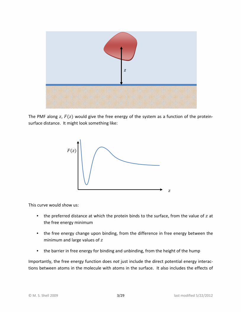
Consider the example of a protein in aqueous solution interacting with a surface. The reaction
coordinate might be the distance between the center of mass of the protein and the surface:
© M. S. Shell 2009 3/29 last modified 5/22/2012
The PMF along ,, *�,� would give the free energy of the system as a function of the protein-
surface distance. It might look something like:
This curve would show us:
• the preferred distance at which the protein binds to the surface, from the value of , at
the free energy minimum
• the free energy change upon binding, from the difference in free energy between the
minimum and large values of ,
• the barrier in free energy for binding and unbinding, from the height of the hump
Importantly, the free energy function does not just include the direct potential energy interac-
tions between atoms in the molecule with atoms in the surface. It also includes the effects of
*�,�
,
,

© M. S. Shell 2009 4/29 last modified 5/22/2012
all of the interactions in the solvent molecules. This may be crucial to the behavior of the
system.
For example, the direct pairwise interactions of an alkane with a silica surface will be the same
regardless of whether the solvent is water or octanol. However, the net interaction of the
alkane and surface will be very different in the two cases due to solvent energies and entropies,
and this effect is exactly determined by the PMF.
Definition
Formally, a potential of mean force (the free energy) along some reaction coordinate + is given
by a partial integration of the partition function. In the canonical ensemble,
*�+� = ���, �, �, +� = −��� ln -��, �, �, +� = −��� ln. � !"$�%&/0+ − +1����2'��
Here, +1���� is a function that returns the value of the order parameter for a particular configu-
ration ��. The integral in this expression entails a delta function that filters for only those
Boltzmann factors for configurations with the specified +.
One can think of the PMF as the free energy when the system is constrained to a given value of +. Notice that we have the identity
.� !3�4�'+ = � !5
The potential of mean force is so-named because it’s derivative gives the average force along
the direction of + at equilibrium. To show this, we need the mathematical identity
''6.7�8�/�8 − 6�'8 = .'7�8�'8 /�8 − 6�'8
Now, we proceed to find the derivative of the PMF:
'*�+�'+ = −��� ''+ ln. � !"$�%&/0+ − +1����2'��
= −���''+ � � !"$�%&/0+ − +1����2'��� � !"��%�/0+ − +1����2'��
= −��� � 9''+ � !"$�%&: /0+ − +1����2'��� � !"��%�/0+ − +1����2'��
© M. S. Shell 2009 5/29 last modified 5/22/2012
= −��� � 9−;'�'+ � !"$�%&: /0+ − +1����2'��� � !"��%�/0+ − +1����2'��
= −�<4� !"$�%&/0+ − +1����2'��� � !"��%�/0+ − +1����2'��
Here, the term <4 gives the force along the direction of +,
<4 = −'�'+
= −'��'+1 ⋅ ∇�
= '��'+1 ⋅ ?�
The remainder of the terms in the PMF equation serve to average the force for a specified value
of +. Thus,
'*�+�'+ = −@<4A�+� Paths
Keep in mind that free energies are state functions. That is, if we are to compute a change in
any free energy between two conditions, we are free to pick an arbitrary path of interest
between them. This ultimately lends flexibility to the kinds of simulation approaches that we
can take to compute free energies.
Overview of histograms in simulation
Until now, we have focused mainly on computing property averages in simulation. Histograms,
on the other hand, are concerned with computing property distributions. These distributions
can be used to compute averages, but they contain much more information than that. Im-
portantly, they relate to the fluctuations in the ensemble of interest, and can ultimately be tied
to statistical-mechanical partition functions. It is through this connection that histograms
enable us to compute free energies and entropies.
Definitions and measurement in simulation
For the purposes of illustration, we will consider a histogram in potential energy. In our simula-
tion, we want to measure the distribution of the variable � using a long simulation run and
many observations of the instantaneous value of �.

© M. S. Shell 2009 6/29 last modified 5/22/2012
In classical systems, the potential energy is a continuously-varying variable. Therefore, the
underlying ℘��� is a continuous probability distribution. However, in the computer we must
measure a discretized version of this distribution.
• We specify a minimum and maximum value of the energy that defines a range of ener-
gies in which we are interested. Let these be �min and �max. • We define a set of G bins into which the energy range is discretized. Each bin has a bin
width of
/� = �max − �minG
• Let the variable � be the bin index. It varies from 0 to G − 1. The average energy of
bin � is then given by
�I = �min + K� + 12M /�
• We create a histogram along the energy bins. This is simply an array in the computer
that measures counts of observations:
NI = countsof�observationsintherangeX�I − /� 2⁄ , �I + /� 2⁄ ) For the sake of simplicity, we will often write the histogram array using the energy, rather than
the bin index,
N(�) = NIwhere� = int K� − �min/� M
Here the int function returns the integer part of its argument. For example, int(2.6) = 2.
To determine a histogram in simulation, we perform a very large number of observations \
from a long, equilibrated molecular simulation. At each observation, we update:
N(�) ← N(�) + 1
This update is only performed if �min ≤ � < �max. Otherwise, the energy would be outside of
the finite range of energies of interest. However, we still need to keep count of all energies,
whether or not inside the range, in order to properly normalize our histogram.
We can normalize the histogram to determine a discretized approximation to the true underly-
ing distribution ℘(�) in the energy range of interest:
© M. S. Shell 2009 7/29 last modified 5/22/2012
℘̀(�)/� = N(�)\
where \ is the total number of observations, including those energies outside of the defined
range. On the LHS we include the bin width so as to approximate the continuous probability
differential ℘(�)'�. Thus,
℘̀(�) = N(�)\/�
In the limit of an infinite number of observations from an infinitely long, equilibrated simula-
tion, this approximation converges to the true one in the following manner:
℘̀(�I)/� = . ℘(�)'�"abc" d⁄"a c" d⁄
This equation simply says that we sum up all of the underlying probabilities for the continuous
energies within a bin to obtain the observed, computed probabilities. As the bin width goes to
zero, we have
limc"→�,f→g ℘̀(�) = ℘(�) Notice that there are two components to this limit:
• We need an infinite number of observations.
• We need an infinite number of bins.
These two limits “compete” with each other: as we increase the number of bins, we need more
observations so that we have enough counts in each bin to have good statistical accuracy.
Practically speaking, we must choose a finite bin width that enables us to balance the length of
the run with statistical accuracy in each bin. Typically, for the energy example above,
• the bin width is chosen to be of the order of a basic energy scale in the force field. For a
Lennard-Jones system, this might be h.
• the simulation is performed long enough to achieve on the order of ~1000 or more av-
erage counts per bin, that is, \ ≥ G × 1000.
Statistical considerations
Keep in mind that the computation of a histogram is subject to the same statistical considera-
tions as simple simulation averages. That is, the histogram needs to be performed for many
© M. S. Shell 2009 8/29 last modified 5/22/2012
correlation times of the energy � in order to reach good statistical accuracy. It can be shown
that the expected squared error in the histogram bin N(�) goes as
lm(")d ∝ N(�) This implies that the error goes as the square root as the number of counts. Similarly, the
expected squared error in the corresponding estimate ℘̀(�) goes as:
l℘̀(")d ∝ ℘(�)\
The relative error in ℘̀(�) is given by: l℘̀(")℘̀(�) ∝ 1o\℘(�) Notice that the relative error is higher for lower values of ℘(�), i.e., at the tails of the distribu-
tion.
Multidimensional histograms
In this example, we considered only a histogram of potential energy. However, it is possible to
construct histograms of many kinds of simulation observables. In other ensembles, we might
compute distributions of other fluctuating macroscopic quantities like � in GCMC simulations
and � in �� simulations. We can also view histograms of arbitrary parameters of interest,
such as the end-to-end distance of a polymer chain or that number of hydrogen bonds a water
molecule makes.
We can also compute joint distributions using multidimensional histogram arrays. For exam-
ple,
℘̀(�, �)/�/� = N(�, �)\
Note that any continuous variables will require discretization and specification of a bin width.
Discrete variables, on the other hand, do not require such a definition because the underlying
distribution itself is discrete:
℘̀(�) = N(�)\
Many kinds of distributions, however, require the specification of a minimum and maximum
observable value.

© M. S. Shell 2009 9/29 last modified 5/22/2012
Connection to statistical mechanics
The true power of histograms is that they allow us to measure fluctuations in the simulation
that can be used to extract underlying partition functions. That is, we measure ℘(�) in simula-
tion and then we post-process this discretized function to make connections to free energies
and entropies.
Consider the energy distribution ℘(�). Its form in the canonical ensemble is given by the
expression:
℘(�) = Ωq(�, �, �)� !"-(�, �, �)
where -(�, �, �) is the configurational partition function,
-(�, �, �) = .Ωq(�, �, �)� !"'�
Here, Ωm is the configurational density of states. It is the part of the microcanonical partition
function that corresponds to the potential energy and configurational coordinates. It is defined
by the equation
Ωm(�, �, �) = ./X�(��) − �r'��
The reason we are concerned only with the configurational energy distribution is that the
kinetic component can always be treated analytically, within the context of equilibrium simula-
tions.
We can rewrite both using the dimensionless configurational entropy:
sm(�, �, �) ≡ lnΩm(�, �, �) ℘(�) = �uv(",w,�) !"-(�, �, �) -(�, �, �) = .�uv(",w,�) !"'�
Basic histogram analysis and reweighting
The above formalism shows that if we were able to compute the function sm(�, �, �), we
would be able to predict the complete energy distribution ℘(�) at any temperature. In fact,
things are a bit simpler than this: we only need the energy-dependence of sm, since the volume
and number of particles stay fixed.
For example, we can compute the average potential energy at any temperature using the
expression

© M. S. Shell 2009 10/29 last modified 5/22/2012
x�y(�) = .�℘(�; �)'�
= .��uv(") !"'�-(�)
= ���uv(") !"'���uv(") !"'�
Here, we use the notation ℘(�; �) to signify a distribution at a given specified temperature �.
Extracting the entropy and density of states from a histogram
We might extract an estimate for sm by measuring ℘(�; �) from a histogram in a canonical
simulation at specified temperature �. Inverting the above relationship,
sm(�) = ln {-(�)℘(�; �)� !" | = ln℘(�; �) + ;� + ln -(�) = ln℘(�; �) + ;� − ;�m(�) Here, �m(�) is the configurational part of the Helmholtz free energy,
�(�, �, �) = �m(�, �, �) + ��� lnX�! Λ(�)��r We can measure ℘(�; �) using a histogram along a set of discrete energies. Post-simulation,
we can then take this measured distribution and use it to compute a discrete approximation to
the dimensionless entropy function at the same energies,
sm(�I) = ln℘(�I; �) + ;�I − ;�m(�) Notice that the partition function part of this expression is a temperature-dependent constant
that is independent of potential energy �. Thus, we can compute the entropy function sm to
within an additive constant using this approach. This also says that we can compute the config-
urational density of states to within a multiplicative constant. This basic inversion of the
probability distribution function underlies many histogram-based methods.
Keep in mind that sm(�) is fundamentally independent of temperature since it stems from the
microcanonical partition function. That is, any temperature-dependencies on the RHS of this
equation should exactly cancel to leave a �-independent function. Another way of putting this
is that, in principle, it does not matter from which temperature we measure ℘(�; �). At
equilibrium, the ℘(�; �) from all temperatures should give the same sm(�) function.

© M. S. Shell 2009 11/29 last modified 5/22/2012
Free energy differences from histograms
Imagine that we measure ℘(�; �) and ℘(�; �d) from two simulations at different tempera-
tures. We can use the relationship of both with the density of states to compute a free energy
difference. We construct
ln℘(�; �d)℘(�; �) = Xsm(�) − ;d� + ;d�m(�d)r − Xsm(�) − ;� + ;�m(�)r = −(;d − ;)� + ;d�m(�d) − ;�m(�) Rearranging,
;d�m(�d) − ;�m(�) = ln℘(�; �d)℘(�; �) + (;d − ;)�
This expression provides us with a way to determine the configurational free energy difference
between temperatures 1 and 2 using measured histograms of the energy distribution.
You may find it interesting that the RHS is dependent on �, whereas the LHS is not. In fact, the
free energies should have no �-dependence. In principle, any value of � could be plugged into
the RHS and the same free energy would be returned. In practice, statistical errors in the
measured ℘(�) mean that the estimate for the free energy can have different accuracies
depending on the value of � chosen. More on this below.
Reweighting
With a computed a discrete approximation to the underlying energy distribution, we can also
use it to predict ℘(�) at temperatures other than the original simulation temperature. This
basic procedure is called reweighting, since we use a distribution measured at one temperature
to predict that at another. The scheme is as follows.
Imagine sm(�) is computed from ℘(�; �) in a canonical simulation at �. We have
sm(�) = ln℘(�; �) + ;� − ;�m(�) We want to predict ℘(�; �d) at another temperature �d. We have,
℘(�; �d) = �uv(") !�"-(�d)
Plugging in the above expression for sm,
℘(�; �d) = ℘(�; �)� (!� !#)" -(�)-(�d)

© M. S. Shell 2009 12/29 last modified 5/22/2012
However, the last term on the RHS involving the ratio of partition functions is independent of �. We can find it using the probability normalization condition,
.℘(�; �d)'� = 1
Thus,
℘(�; �d) = ℘(�; �)� (!� !#)"�℘(�; �)� (!� !#)" '�
This equation is an important one. It states that a distribution measured at � can be used to
predict a distribution at a different �d. Thus, in principle, we would only need to perform a
single simulation, measure ℘(�) once, and use this expression to examine the energy distribu-
tion at any other temperature of interest. For example, we might compute the average energy
as a function of temperature using the equation
x�y(�d) = .�℘(�; �d)'�
= ��℘(�; �)� (!� !#)" '��℘(�; �)� (!� !#)" '�
Similar expressions could be found for other moments of the potential energy, such as x�dy. These could be used to compute the temperature dependence of the heat capacity, using the
relationship ���d�w = x�dy − x�yd. Statistical analysis
Unfortunately, there are practical limits to the histogram reweighting procedure just described.
The main problem is the measurement of ℘(�) to good statistical accuracy in the tails of its
distribution. Consider that a typical ℘(�) is very sharply peaked:
℘(�)
�

© M. S. Shell 2009 13/29 last modified 5/22/2012
The width of the distribution relative to the mean goes roughly as � #� so that, for macroscopic
systems, the distribution is infinitely peaked.
The implication of this result is that it is very hard to measure the distribution at it tails, where
we typically only have a few counts in each bin. If we reweight a measured distribution to a
temperature where the tails change to high probability, the error can be magnified to be very
large.
Here, the mean of the distribution at the new temperature is well within the tail region of the
distribution at the original temperature. If we reweight ℘(�; �) to �d, errors in the tails will be
magnified. The error in the new distributions can be written approximately as
l℘(";��)d ≈ l℘(";�#)d �℘(�; �d)℘(�; �)�d
This formula is derived using standard error propagation rules and the reweighting expression.
Notice that if �d = �d, the error is the same at each energy as from the original measurement.
Otherwise, we must weigh the error by a ratio involving the two probability distributions. In
the above picture, the ratio
℘(�∗; �d)℘(�∗; �) is very large due to the small probability of this energy at �. Therefore, the error is greatly
magnified in the reweighting procedure according to the above equation.
In general,
• Distributions are subject to statistical inaccuracies at their tails, owing to the finite
number of counts in each bin.
℘(�)
�
�d > �
�
�∗
© M. S. Shell 2009 14/29 last modified 5/22/2012
• If the important parts of the energy distribution at �d correspond to the tails of a meas-
ured distribution at �, a reweighting procedure will fail due to large statistical errors.
• If computed from a measured ℘(�; �), the quality of an estimated sm(�) function is
only good around the frequently-sampled energies, i.e., for energies where the histo-
gram has many entries.
These techniques limit the determination of free energies and entropies using measurements
from single histograms. The solution here, as we will see next, it to incorporate multiple
histogram estimates of these quantities.
Multiple histogram reweighting
For the remainder of this section we will drop the subscript “c” from the configurational prop-
erties, for simplicity.
Imagine that we were able to take histograms from multiple simulations �, each at a different
temperature ��. For each, we could get a different estimate of the underlying dimensionless
configurational entropy function s:
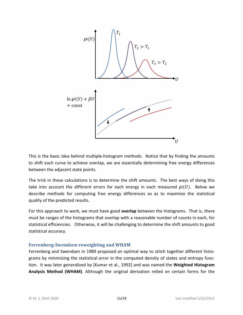
s(�) = ln℘(�; ��) + ;�� − ;��(��) We should get the same function every time. We don’t know the free energies, but we do
know that these are merely additive constants in the entropy functions. We can therefore shift
the different estimates for the entropy function up or down in value until they all match each
other:
© M. S. Shell 2009 15/29 last modified 5/22/2012
This is the basic idea behind multiple-histogram methods. Notice that by finding the amounts
to shift each curve to achieve overlap, we are essentially determining free energy differences
between the adjacent state points.
The trick in these calculations is to determine the shift amounts. The best ways of doing this
take into account the different errors for each energy in each measured ℘(�). Below we
describe methods for computing free energy differences so as to maximize the statistical
quality of the predicted results.
For this approach to work, we must have good overlap between the histograms. That is, there
must be ranges of the histograms that overlap with a reasonable number of counts in each, for
statistical efficiencies. Otherwise, it will be challenging to determine the shift amounts to good
statistical accuracy.
Ferrenberg-Swendsen reweighting and WHAM
Ferrenberg and Swendsen in 1989 proposed an optimal way to stitch together different histo-
grams by minimizing the statistical error in the computed density of states and entropy func-
tion. It was later generalized by [Kumar et al., 1992] and was named the Weighted Histogram
Analysis Method (WHAM). Although the original derivation relied on certain forms for the
℘(�)
�
�d > �
�
�� > �d
ln℘(�) + ;�+ const
�
© M. S. Shell 2009 16/29 last modified 5/22/2012
error propagation, the same result can be derived using a more elegant maximum likelihood
approach, which is what we discuss here.
The maximum likelihood approach is a statistical method for parameterizing probability mod-
els. It simply says the following: posit some form of the underlying distribution function for a
random process. Then, given an observed set of events, the best parameters for that distribu-
tion are those that maximize the probability (likelihood) of the observed events.
In this context, imagine we are trying to determine Ω(�) from � simulations at different tem-
peratures ��. We know that the underlying Ω(�) for each should be the same, but that the
measured histograms N�(�) will be different because the simulations are performed at different
temperatures. The observed events are the energies tabulated in the histograms.
Say that we make \ independent observations of the energy � in each temperature. Here,
independent implies that we are beyond twice the correlation time. In order to make a connec-
tion with the histogram, we will discretize all of energy space into discrete values �I separated
by intervals /�. Before we start, let’s define some notation:
• \ – number of observations at each temperature
• � – index of observations (� = 1,… , \) • � – index of temperature (� = 1,… , �) • � – index of discrete energy values
• �I – discrete energy values
• ΩI, sI – density of states and entropy at the values �I
• ��� – energy of the �th observation at temperature � • N�I– count of histogram entries for temperature � and energy bin �
Derivation
With these notations, we construct the total probability or likelihood � of making the \� obser-
vations from the simulations in terms of a yet-unknown unknown density of states function:
� =��℘(���; ��)���
f��
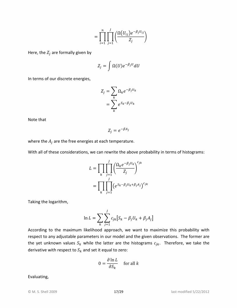
© M. S. Shell 2009 17/29 last modified 5/22/2012
=���Ω$���&� !�"��-� ����
f��
Here, the -� are formally given by
-� = .Ω(�)� !�"'�
In terms of our discrete energies,
-� =�ΩI� !�"aI
=��ua !�"aI
Note that
-� = � !5� where the �� are the free energies at each temperature.
With all of these considerations, we can rewrite the above probability in terms of histograms:
� =���ΩI� !�"a-� �m�a���I
=��$�ua !�"ab!�5�&m�a���I
Taking the logarithm,
ln � =��N�I0sI − ;��I + ;���2���I
According to the maximum likelihood approach, we want to maximize this probability with
respect to any adjustable parameters in our model and the given observations. The former are
the yet unknown values sI while the latter are the histograms N�I. Therefore, we take the
derivative with respect to sI and set it equal to zero:
0 = � ln ��sI forall�
Evaluating,

© M. S. Shell 2009 18/29 last modified 5/22/2012
0 =��N�I + \;� ����sI����
The latter derivative is
;� ����sI = −� ln-��sI
= −�ua !�"a-�
Substituting back in:
0 =�$N�I − \�ua !�"ab!�5�&��� forall�
This equation can be solved for sI:
�ua = ��N�I��� � �\�� !�"ab!�5��
�� �
Notice that this equation now provides us with a recipe for computing the density of states (the
LHS) based on histogram data. Let’s rewrite it without the index � for clarity:
�u�"� = N������\ ��� !�"b!�5���� �
Here, we have made the definition that N������ gives the total number of histogram counts of
energy �, at any temperature.
Even though this expression gives us a way to determine the entropy function from multiple
simulation results, note that the RHS involves the free energy at every temperature. This free
energy depends on the entropy itself:
�� = −;� ln��u�"� !�""
Iterative solution
How can we solve for s���? Ferrenberg and Swendsen suggested an iterative solution:
1. An initial guess is made for the � values of ��. One can simply choose �� = 0 for all �.

© M. S. Shell 2009 19/29 last modified 5/22/2012
2. The (discretized) entropy at every energy is computed using
s(�) = ln N���(�) − ln \ − ln�� !�"b!5���� forall�
3. The free energies are recalculated using
−;��� = ln��u�"� !�"" forall� 4. Steps 2 and 3 are repeated until the free energies no longer change upon each iteration.
In practice, one typically checks to see if the free energies change less than some frac-
tional tolerance.
5. According to the above equations, the entropy function and the combinations ;��� can-
not be determined to within more than an additive constant. Thus, with each iteration,
one typically sets one of the free energies equal to zero at one temperature, ��� = 0.
This iterative procedure can be fairly computationally expensive since it involves sums over all
temperatures and all discretized energies with each iteration. It is not uncommon to require on
the order of 100-1000 iterations to achieve good convergence.
However, once convergence has been achieved, energy averages at any temperature—even
temperatures not included in the original dataset—can be computed with the expression
℘��; �� ∝ �u�"� !"
The constant of proportionality is determined by normalizing the probability distribution.
This general approach is termed multiple histogram reweighting, and it can be shown to be the
statistically optimal method for reweighting data from multiple simulations. That is, it makes
the maximum use of information and results in reweighted distributions for ℘��; �� that have
the least statistical error. Importantly, it provides statistically optimal estimates of free energy
differences �� − ��b.
Configurational weights
Using the multiple histogram technique, it is possible to define a weight associated with each
configuration � at each temperature � at the reweighting temperature �:
��� = �u�"��� !"��N���$���&
© M. S. Shell 2009 20/29 last modified 5/22/2012
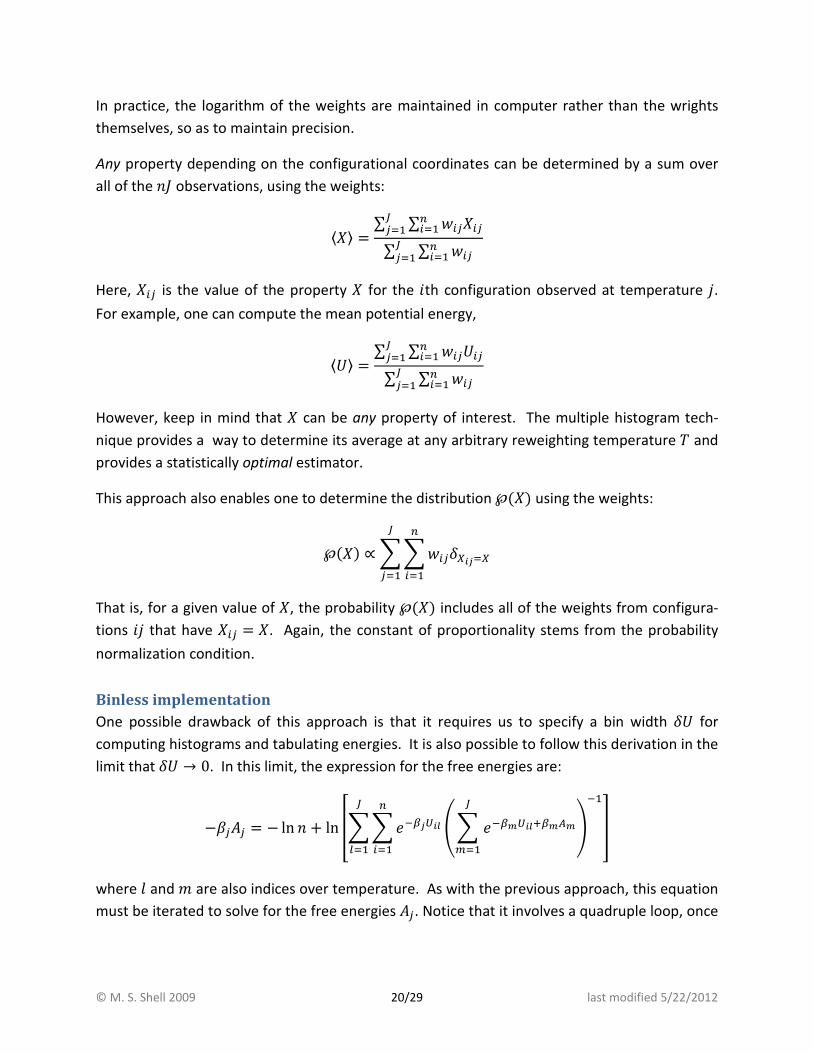
In practice, the logarithm of the weights are maintained in computer rather than the wrights
themselves, so as to maintain precision.
Any property depending on the configurational coordinates can be determined by a sum over
all of the \� observations, using the weights:
x�y = ∑ ∑ ������f�����∑ ∑ ���f�����
Here, ��� is the value of the property � for the �th configuration observed at temperature �. For example, one can compute the mean potential energy,
x�y = ∑ ∑ ������f�����∑ ∑ ���f�����
However, keep in mind that � can be any property of interest. The multiple histogram tech-
nique provides a way to determine its average at any arbitrary reweighting temperature � and
provides a statistically optimal estimator.
This approach also enables one to determine the distribution ℘(�) using the weights:
℘(�) ∝�����/�����f��
���
That is, for a given value of �, the probability ℘(�) includes all of the weights from configura-
tions �� that have ��� = �. Again, the constant of proportionality stems from the probability
normalization condition.
Binless implementation
One possible drawback of this approach is that it requires us to specify a bin width /� for
computing histograms and tabulating energies. It is also possible to follow this derivation in the
limit that /� → 0. In this limit, the expression for the free energies are:
−;��� = − ln \ + ln ���� !�"�� �� � ! "��b! 5 �¡� ¢ f
���£� ¤
where ¥ and G are also indices over temperature. As with the previous approach, this equation
must be iterated to solve for the free energies ��. Notice that it involves a quadruple loop, once
© M. S. Shell 2009 21/29 last modified 5/22/2012
over observations and three times over temperatures. Therefore, convergence can be much
slower than the histogram version.
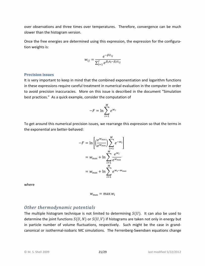
Once the free energies are determined using this expression, the expression for the configura-
tion weights is:
��� = � !"��∑ �!�5� !�"���£�
Precision issues
It is very important to keep in mind that the combined exponentiation and logarithm functions
in these expressions require careful treatment in numerical evaluation in the computer in order
to avoid precision inaccuracies. More on this issue is described in the document “Simulation
best practices.” As a quick example, consider the computation of
−* = ln��¦����
To get around this numerical precision issues, we rearrange this expression so that the terms in
the exponential are better-behaved:
−* = ln §K�¦max�¦maxM�� ¦���� ¨
= �max + ln� �¦��¦max���
= �max + ln��¦� ¦max���
where
�max = max�� Other thermodynamic potentials
The multiple histogram technique is not limited to determining s(�). It can also be used to
determine the joint functions s(�, �) or s(�, �) if histograms are taken not only in energy but
in particle number of volume fluctuations, respectively. Such might be the case in grand-
canonical or isothermal-isobaric MC simulations. The Ferrenberg-Swendsen equations change
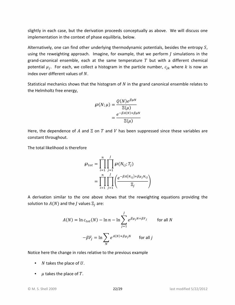
© M. S. Shell 2009 22/29 last modified 5/22/2012
slightly in each case, but the derivation proceeds conceptually as above. We will discuss one
implementation in the context of phase equilibria, below.
Alternatively, one can find other underlying thermodynamic potentials, besides the entropy s,
using the reweighting approach. Imagine, for example, that we perform � simulations in the
grand-canonical ensemble, each at the same temperature � but with a different chemical
potential ©�. For each, we collect a histogram in the particle number, N�I where � is now an
index over different values of �.
Statistical mechanics shows that the histogram of � in the grand canonical ensemble relates to
the Helmholtz free energy,
℘(�; ©) = ª(�)�!«�Ξ(©)
= � !5(�)b!«�Ξ(©)
Here, the dependence of � and Ξ on � and � has been suppressed since these variables are
constant throughout.
The total likelihood is therefore
℘��� =��℘(���; ��)���
f��
=���� !5$���&b!«����Ξ� )���
f��
A derivation similar to the one above shows that the reweighting equations providing the
solution to �(�) and the � values Ξ� are:
�(�) = ln N���(�) − ln \ − ln��!«��b!3���� for all �
−;*� = ln��5(�)b!«��� for all � Notice here the change in roles relative to the previous example
• � takes the place of �.
• © takes the place of �.

© M. S. Shell 2009 23/29 last modified 5/22/2012
• Instead of computing s(�), we compute the underlying function �(�). That is, we find
the partition function corresponding to variations in � fluctuations at constant �, since
all of our simulations were at the same temperature.
• We compute *� = −��� ln Ξ� at each chemical potential, rather than �� at each tem-
perature. By statistical mechanics, *� = −��. Thus, the differences between these
weights provide information about the pressure differences.
It is possible to determine many different kinds of free-energetic quantities in this way. In
general,
• To compute a free energy or entropy * as a function of some macroscopic parameter �,
the simulation must accomplish fluctuations in �. For example, �(�) requires fluctua-
tions in � and thus would necessitate use of the isothermal-isobaric ensemble.
• To have good statistical accuracy, a wide range of fluctuations in � must be sampled.
This can be accomplished by performing multiple simulations at different values of the
parameter conjugate to �. To compute �(�), different pressures would be imposed
for multiple simulations at the same temperature.
• The multiple-histogram reweighting procedure will compute *(�) as well as the relative
partition functions at the different simulation conditions. In the example for �(�), we
would find �(�) as well as ��, where � is the Gibbs free energy of the isothermal-
isobaric ensemble.
Potentials of mean force (PMFs)
The connection between a PMF and simulation observables stems from the probability distribu-
tion of the reaction coordinate of interest. Based upon the fact that the total partition function
can be expressed as a sum over the PMF partition function, we have that
℘(+) = � !3(4)-
That is, the probability that one will see configurations with any value of + is proportional to a
Boltzmann factor involving the potential of mean force at +.
This approach enables us to measure PMFs in simulation by computing histograms along
reaction coordinates. We have,
*(+) = −��� ln℘(+) − ��� ln - = −��� ln℘(+) + const
© M. S. Shell 2009 24/29 last modified 5/22/2012
Notice that - provides an additive constant independent of the reaction coordinate. Typically,
we cannot determine the PMF in absolute units, which would require the determination of the
absolute free energy of the system. Instead, we can only compute *(+) curves to within an
additive constant. This is not normally a problem, however, since we are usually only interest-
ed in relative free energies along +.
One of the limitations of this basic approach is that we cannot compute large changes in free
energies due to the statistics of the histogram. Imagine that we examine a free energy differ-
ence at two values of +, *(+d) − *(+). Say that this value is equal to 4���, which is a moder-
ate energy equal to about 2 kcal/mol at room temperature. The relative probabilities at these
two values would be
℘(+d)℘(+) = � !$3(4�) 3(4#)& = � ® ≈ 0.02
If we were to measure a histogram and the bin for + contained 1000 entries, the bin for +d
would only contain ~20 entries. Thus, the statistical error for the latter would be quite high.
The main point here is that it is difficult to measure free energies for rarely sampled states.
One way around this, which we will discuss in a later lecture, is to bias our simulation to visit
these states. Though the introduction of the bias modifies the ensemble we are in, we can
exactly account for this fact in the computation of thermodynamic properties.
Weighted Histogram Analysis Method (WHAM)
If multiple simulations are performed at different state conditions (e.g., different �,, or ©), the
Ferrenberg-Swendsen reweighting approach can also be used to compute potentials of mean
force at some set of target conditions. This is quite straightforward.
As before, imagine that � simulations are performed at different conditions. In each simulation �, \ observations � are made. In addition to computing the energy, one tallies the value of the
reaction coordinate for each observation:
+�� Then, the PMF at some final set of conditions (the reweighting temperature, chemical potential,
and/or pressure) is found by tallying the configurational weights to compute the distribution in +:

© M. S. Shell 2009 25/29 last modified 5/22/2012
℘(+) ∝�����/4���4f��
���
Ultimately, this distribution will need to be performed in a discretized array if + is a continuous
variable. Then, the PMF simply comes from
*(+) = −��� ln℘(+) Histogram methods for computing phase equilibria
The computation of phase equilibria—saturation conditions, critical points, phase diagrams,
etc.—is a major enterprise in the molecular simulation community. There are many ways that
one might go about this, including the Gibbs ensemble, and they are discussed in detail in
[Chipot & Pohorille, Free Energy Calculations: Theory and Applications in Chemistry and Biolo-
gy, Springer, 2007]. Of all of these methods, however, the current gold-standard for phase
equilibrium computations is one that relies on multiple histogram reweighting. This approach is
often the quickest and has the maximum accuracy.
Here we will discuss these calculations in the context of liquid-vapor equilibria. Other phase
behavior—such as liquid-solid, vapor-solid, or liquid-liquid (in mixtures)—can be treated using
this approach as well, although special techniques may be needed to treat structured phases.
Grand canonical perspective
The basic idea of our calculations is the following:
• For a given temperature, we want to find the conditions at which phase equilibrium oc-
curs. In a single component system, we only have one free parameter to specify this
condition in addition to �, per the Gibbs phase rule. This could be or ©.
• We will focus on © instead of and perform simulations in the grand canonical ensem-
ble. Thus, we want to find the value of © at coexistence that generates an equilibrium
between liquid and vapor phases. We could equally choose and perform �� simula-
tions; however, particle insertions and deletions are generally much more efficient than
volume fluctuations and thus we go with the former for computational reasons.
• If the state conditions place us at conditions of phase equilibrium (i.e., on the liquid-
vapor phase line), we expect the GCMC simulation to spontaneously fluctuate between
a dense liquid (low �, large �) and dilute gas (high �, small �). These fluctuations can
be observed by examining the joint distribution
℘(�,�)
© M. S. Shell 2009 26/29 last modified 5/22/2012
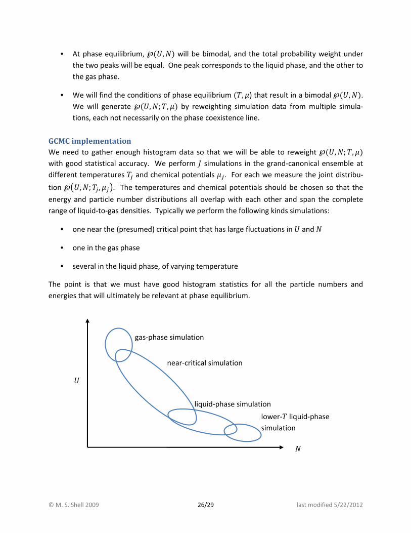
• At phase equilibrium, ℘(�,�) will be bimodal, and the total probability weight under
the two peaks will be equal. One peak corresponds to the liquid phase, and the other to
the gas phase.
• We will find the conditions of phase equilibrium (�, ©) that result in a bimodal ℘(�,�). We will generate ℘(�,�; �, ©) by reweighting simulation data from multiple simula-
tions, each not necessarily on the phase coexistence line.
GCMC implementation
We need to gather enough histogram data so that we will be able to reweight ℘(�, �; �, ©) with good statistical accuracy. We perform � simulations in the grand-canonical ensemble at
different temperatures �� and chemical potentials ©�. For each we measure the joint distribu-
tion ℘$�,�; �� , ©�&. The temperatures and chemical potentials should be chosen so that the
energy and particle number distributions all overlap with each other and span the complete
range of liquid-to-gas densities. Typically we perform the following kinds simulations:
• one near the (presumed) critical point that has large fluctuations in � and �
• one in the gas phase
• several in the liquid phase, of varying temperature
The point is that we must have good histogram statistics for all the particle numbers and
energies that will ultimately be relevant at phase equilibrium.
�
�
near-critical simulation
gas-phase simulation
liquid-phase simulation
lower-� liquid-phase
simulation
© M. S. Shell 2009 27/29 last modified 5/22/2012
Once these histograms are taken, Ferrenberg-Swendsen iterations are used to compute the
free energy at each state point. The relevant equations for GCMC simulations are:
s��, �� � ln N�����, �� � ln \ � ln � � !�"b!�«��b!�3��
�� for all �, �
�;*� � ln � � �u�",�� !�"b!�«���"
for all �
This procedure is performed until values for the discretized entropy s��, �� and free energies
*� � ����� ln � converge. Keep in mind that one value of * must be set equal to zero.
Once these values are determined, the joint distribution ℘��, �� can be computed for an
arbitrary reweighting �, © using
℘��, �; �, ©� ∝ �u�",�� !"b!«�
The constant of proportionality is given by the normalization condition.
Using the reweighting equation, one finds phase equilibrium by adjusting © given a value of �
until a bimodal distribution appears and the integral under each peak (the total probability) is
the same. Notice that this is a very fast operation since the Ferrenberg-Swendsen reweighting
only needs to be performed once, at the beginning, to determine s��, ��.
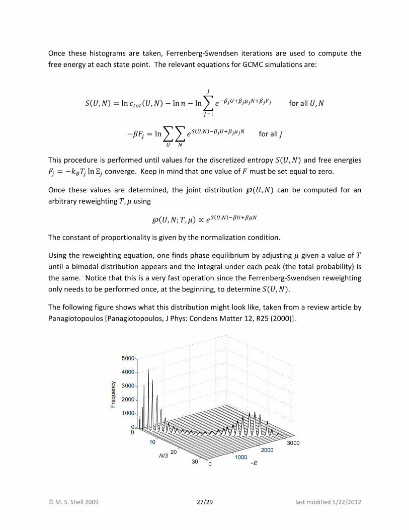
The following figure shows what this distribution might look like, taken from a review article by
Panagiotopoulos [Panagiotopoulos, J Phys: Condens Matter 12, R25 (2000)].

© M. S. Shell 2009 28/29 last modified 5/22/2012
By repeating this procedure at different reweighting temperatures, one can map out the phase
diagram. In the �-¯ plane, this might look like:
The average density of each phase can be determined using:
x¯y° = 1�
∑ ∑ �℘��, ���±�∗"∑ ∑ ℘��, ���±�∗"
x¯y² = 1�
∑ ∑ �℘��, ���³�∗"∑ ∑ ℘��, ���³�∗"
Here, �∗ is the value of � at the minimum between the two peaks in the distribution.
Pressures can be found using the fact that
;� � ln Ξ�©, �, ��
We cannot compute absolute pressures using this equation, because we cannot compute Ξ
absolutely (one must be set to zero). However, we can compare the pressures of two different
state points:
;dd� � ;� � ln Ξ�©d, �d, ��Ξ�©, �, ��
� ln ∑ ∑ �u�",�� !�"b!�«���"∑ ∑ �u�",�� !#"b!#«#��"
By letting one state point correspond to a very dilute, high temperature gas phase, we can
compute its absolute pressure using the ideal gas law. This equation then can be used to relate
the pressure at other state points back to the ideal gas reference.
© M. S. Shell 2009 29/29 last modified 5/22/2012
Critical point reweighting and finite-size scaling
How can one predict the location of the critical point? It turns out that systems have a kind of
universal behavior at this point in the phase diagram. For many fluids, their behavior at the
critical point follows the same trends as the three-dimensional Ising model (or, equivalently,
the lattice gas); that is, they fall in the Ising universality class or the Ising criticality class. In
particular, the probability distribution ℘��, �� assumes a universal form.
We can locate the true critical point by finding reweighting values of �m , ©m so that ℘��, ��
maps onto the universal Ising distribution, which has been computed to high accuracy by a
number of researchers.
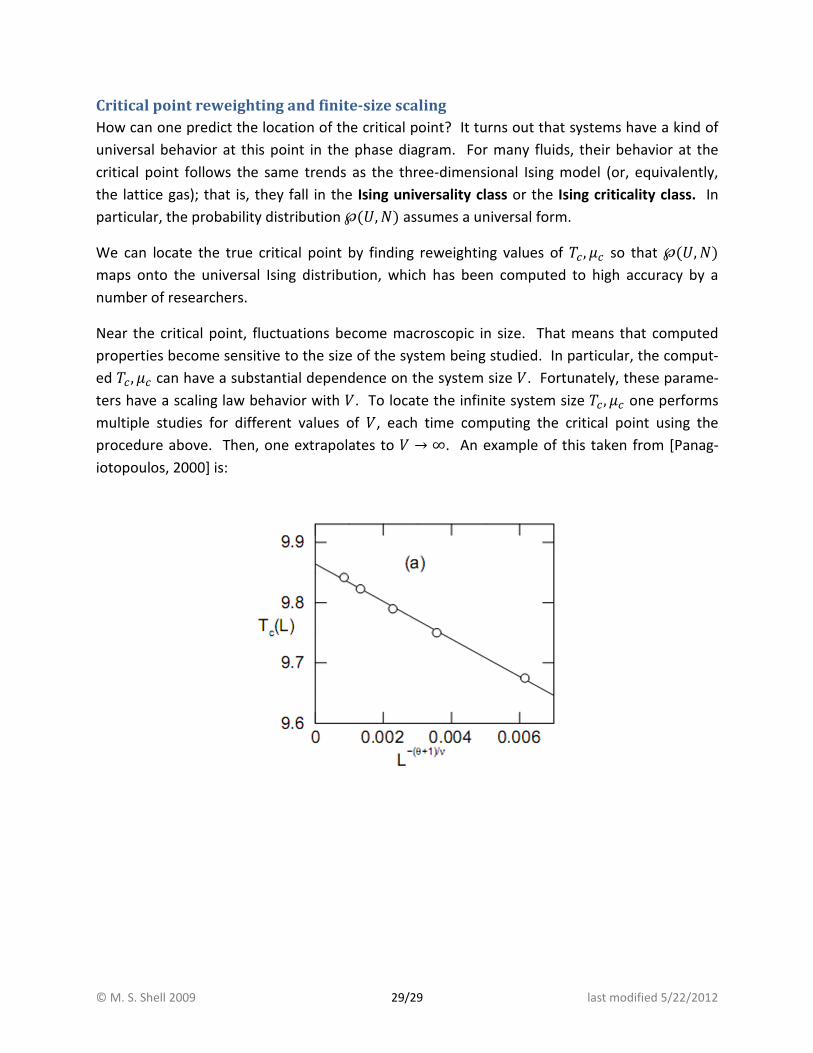
Near the critical point, fluctuations become macroscopic in size. That means that computed
properties become sensitive to the size of the system being studied. In particular, the comput-
ed �m , ©m can have a substantial dependence on the system size �. Fortunately, these parame-
ters have a scaling law behavior with �. To locate the infinite system size �m , ©m one performs
multiple studies for different values of �, each time computing the critical point using the
procedure above. Then, one extrapolates to � → ∞. An example of this taken from [Panag-
iotopoulos, 2000] is: